Contents Introductioncvgmt.sns.it/media/doc/paper/4327/NLE3.pdf · ON THE CONVERGENCE RATE OF SOME...
21
ON THE CONVERGENCE RATE OF SOME NONLOCAL ENERGIES ANTONIN CHAMBOLLE, MATTEO NOVAGA, AND VALERIO PAGLIARI Abstract. We study the rate of convergence of some nonlocal functionals recently considered by Bourgain, Brezis and Mironescu. In particular, we establish the Γ-convergence of the corresponding rate functionals, suitably rescaled, to a limit functional of second order. Contents 1. Introduction 1 2. Finite difference functionals in the 1-dimensional case 3 2.1. Pointwise limit and upper bound 3 2.2. Lower bound in the strongly convex case 5 3. Γ-limit in arbitrary dimension 10 3.1. Slicing and upper bound 11 3.2. Lower bound and compactness 13 References 21 1. Introduction We are interested in the rate of converge, as h & 0, of the nonlocal functionals F h (u) := ˆ R d ˆ R d K h (z)f |u(x + z) - u(x)| |z| dzdx, to the limit functional F 0 (u) := ˆ R d ˆ R d K(z)f (|∇u(x) · ˆ z|)dzdx. Here f : R → [0, +∞) is a convex function of class C 2 satisfying f (0) = f 0 (0) = 0, K : R d → [0, +∞) is a kernel such that K(z)= K(-z) for a.e. z ∈ R d , and ˆ R d K(z) ( 1+ |z| 2 ) dz < +∞, and we set K h (z) := h -d K(z/h). It has been proved by Bourgain, Brezis and Mironescu in [3] that F h (u) tends to F 0 (u) as h & 0 for all u ∈ H 1 (R d ), and in [8,11] (see also [2]) it is shown that such convergence also holds in the sense of Γ-convergence [4, 6], with respect to the L 2 (R d )-topology. Let now (1) E h (u) := F 0 (u) -F h (u) h 2 = 1 h 2 ˆ R d ˆ R d K(z)f (|∇u(x) · ˆ z|) - K h (z)f |u(x + z) - u(x)| |z| dzdx 1
Transcript of Contents Introductioncvgmt.sns.it/media/doc/paper/4327/NLE3.pdf · ON THE CONVERGENCE RATE OF SOME...

ON THE CONVERGENCE RATE OF SOME NONLOCAL ENERGIES
ANTONIN CHAMBOLLE, MATTEO NOVAGA, AND VALERIO PAGLIARI
Abstract. We study the rate of convergence of some nonlocal functionals recently considered by Bourgain,Brezis and Mironescu. In particular, we establish the Γ-convergence of the corresponding rate functionals,suitably rescaled, to a limit functional of second order.
Contents
1. Introduction 12. Finite difference functionals in the 1-dimensional case 32.1. Pointwise limit and upper bound 32.2. Lower bound in the strongly convex case 53. Γ-limit in arbitrary dimension 103.1. Slicing and upper bound 113.2. Lower bound and compactness 13References 21
1. Introduction
We are interested in the rate of converge, as h 0, of the nonlocal functionals
Fh(u) :=
ˆRd
ˆRd
Kh(z)f
(|u(x+ z)− u(x)|
|z|
)dzdx,
to the limit functional
F0(u) :=
ˆRd
ˆRd
K(z)f(|∇u(x) · z|)dzdx.
Here f : R → [0,+∞) is a convex function of class C2 satisfying f(0) = f ′(0) = 0, K : Rd → [0,+∞) is akernel such that K(z) = K(−z) for a.e. z ∈ Rd, andˆ
Rd
K(z)(1 + |z|2
)dz < +∞,
and we set Kh(z) := h−dK(z/h).It has been proved by Bourgain, Brezis and Mironescu in [3] that Fh(u) tends to F0(u) as h 0 for
all u ∈ H1(Rd), and in [8, 11] (see also [2]) it is shown that such convergence also holds in the sense ofΓ-convergence [4, 6], with respect to the L2(Rd)-topology.
Let now
(1) Eh(u) :=F0(u)−Fh(u)
h2=
1
h2
ˆRd
ˆRd
[K(z)f(|∇u(x) · z|)−Kh(z)f
(|u(x+ z)− u(x)|
|z|
)]dzdx
1
2 A. CHAMBOLLE, M. NOVAGA, AND V. PAGLIARI
be the functional which measures the rate of convergence of Fh to F0. In this paper, under the assumptionthat the function f is strongly convex (see condition (12) below), we prove that the family Eh Γ-converges,with respect to the H1(Rd)-topology, to the second order limit functional
E0(u) :=
1
24
ˆRd
ˆRd
K(z) |z|2 f ′′(|∇u(x) · z|)∣∣∇2u(x)z · z
∣∣2 dzdx if u ∈ H2(Rd),
+∞ otherwise,
where z = z/|z|. The uniform convexity assumption on f , which is needed for the Γ-liminf inequality,excludes from our analysis some interesting cases such as f(x) = |x|p with p ≥ 1, p 6= 2. In particular, whenf(x) = |x| and K is radially symmetric, the problem is related to a geometric problem considered in [9] inthe context of a physical model for liquid drops with dipolar repulsion. We also observe that the problem westudy is different from a higher order Γ-limit of Fh (see [5]), which would rather correspond to consideringthe Γ-limit of the functionals
Fh −minF0
hαfor some α > 0 .
As a consequence of our result (see Remark 4) we also get that, if the rate of convergence of Fh(u) toF0(u) is fast enough, more precisely if |Eh(u)| ≤M for all h’s sufficiently small, then u ∈ H2(Rd).
We notice that our result is reminiscent to the one obtained by Peletier, Planqué and Röger in [10],motivated by a model for bilayer membranes, where they consider the convolution functionals
Gh(u) :=
ˆRd
f (Kh ∗ u) dx,
which converge to the functional G0(u) = c´Rd f (u) dx as h 0, where c = c(K, d) is a positive constant,
and show that the corresponding rate functionals
(2)G0(u)− Gh(u)
h2=
1
h2
ˆRd
(c f (u)− f (Kh ∗ u)
)dx
converge pointwise to the limit functional1
2
ˆRd
ˆRd
K(z)|z|2f ′′(u(x))|∇u(x) · z|2dzdx for u ∈ H1(Rd).
In particular, the rate functionals are uniformly bounded if and only if u ∈ H1(Rd).In the proof of our convergence result, we follow a strategy similar to the one in [7,8]: we first consider a
related 1-dimensional problem, and then reduce the general case to it by a slicing procedure. More precisely,in Section 2 we study the functionals
Eh(u) :=1
h2
ˆR
[f(u(x))− f
( x+h
x
u(y)dy
)]dx,
which are a particular case of (2), and we show their convergence (see Theorem 1) to the limit energy
E0(u) :=1
24
ˆRf ′′(u(x)) |u′(x)|2 dx for u ∈ H1(R).
Then, in Section 3 we consider the general functionals in (1) and we prove the Γ-convergence to E0 (seeTheorem 2), which is the main result of this paper. We first show the convergence for d = 1, using the resultof Section 2, and then we reduce to the 1-dimensional case by means of a delicate slicing technique.Acknowledgements. MN and VP are members of INDAM-GNAMPA, and acknowledge partial supportby the Unione Matematica Italiana and by the University of Pisa via Project PRA 2017 Problemi di ottimiz-zazione e di evoluzione in ambito variazionale. Part of this work was done during a visit of the third authorto the Ecole Polytechnique.
ON THE CONVERGENCE RATE OF SOME NONLOCAL ENERGIES 3
2. Finite difference functionals in the 1-dimensional case
For u ∈ L2(R) and h > 0, we define the energy
(3) Eh(u) :=1
h2
ˆR
[f(u(x))− f (DhU(x))] dx,
where
(4) U(x) :=
ˆ x
0
u(y)dy and DhU(x) :=U(x+ h)− U(x)
h=
x+h
x
u(y)dy.
Let us fix an open interval I := (a, b) ⊂ R. We shall compute the Γ-limit of Eh regarded as a familyof functionals on the closed subspace Y ⊂ L2(R) defined as
(5) Y := u ∈ L2(R) : u = 0 in R \ I
endowed with the L2-topology. Let us set
(6) E0(u) :=
1
24
ˆRf ′′(u(x)) |u′(x)|2 dx if u ∈ Y ∩H1(R),
+∞ otherwise.
We shall prove the following:
Theorem 1. Let us assume that there exists γ > 0 such that 2f(t)− γt2 is convex. Then, the restriction toY of the family Eh Γ-converges, as h 0, to E0 w.r.t. the L2(R)-topology, that is, for every u ∈ Y thefollowing properties hold:
(1) For any family uh ⊂ Y that converges to u in L2(R) we have
E0(u) ≤ lim infh0
Eh(uh).
(2) There exists a sequence uh ⊂ Y converging to u in L2(R) such that
lim suph0
Eh(uh) ≤ E0(u).
The Γ-upper limit is established in Proposition 1, while Proposition 2 takes care of the lower limit. In turn,the latter is achieved by exploiting a suitable lower bound on the energy (see Lemma 1) and a compactnessresult (see Lemma 2).
2.1. Pointwise limit and upper bound. We now compute the limit of Eh(u), as h 0, for a functionu ∈ Y ∩ C2(R).
Proposition 1. Let u ∈ Y ∩ C2(R). Then, there exists a continuous, bounded, and increasing functionm : [0,+∞)→ [0,+∞) such that m(0) = 0 and
(7) |Eh(u)− E0(u)| ≤ cm(h),
where c := c(b− a, ‖u‖C2(R), ‖f‖C2([−‖u‖C2(R),‖u‖C2(R)])) > 0 is a constant. In particular,
limh0
Eh(u) = E0(u),
moreover for every u ∈ Y there exists a sequence uh ⊂ Y that converges to u in L2(R) and satisfies
lim suph0
Eh(uh) ≤ E0(u).
4 A. CHAMBOLLE, M. NOVAGA, AND V. PAGLIARI
Proof. Since u ∈ Y ∩ C2(R) and f ∈ C2(R), it is easy to see that Fh(u) − F0(u) and E0(u) are uniformlybounded in h. Thus, there exists a constant c∞ > 0 such that
(8) |Eh(u)− E0(u)| ≤ c∞ for h > 1.
Next, we focus on the case h ∈ (0, 1]. If x /∈ (a− h, b), then DhU(x) = 0, and hence
F0(u)− Fh(u) =
ˆ b
a
[f(u(x))− f (DhU(x))] dx−ˆ a
a−hf(DhU(x))dx.
Being u regular, for any x ∈ (a− h, b) we have the Taylor’s expansion
DhU(x) = u(x) +h
2u′(x) +
h2
6u′′(xh), with xh ∈ (x, x+ h),
which we rewrite as
(9) DhU(x) = u(x) + hvh(x), with vh(x) :=u′(x)
2+h
6u′′(xh);
note that vh converges uniformly to u′/2 as h 0.Plugging (9) into the definition of Fh, we get
F0(u)− Fh(u) =−ˆ b
a
[f(u(x) + hvh(x)
)− f(u(x))
]dx−
ˆ a
a−hf
(h2
6u′′(xh)
)dx
=− hˆ b
a
f ′(u(x))vh(x)dx− h2
2
ˆ b
a
f ′′(wh(x))vh(x)2dx
−ˆ a
a−hf
(h2
6u′′(xh)
)dx,
where wh fulfils wh(x) ∈ (u(x), u(x) + hvh(xh)) for all x ∈ (a, b).It easy to see that ∣∣∣∣ˆ a
a−hf
(h2
6u′′(xh)
)dx
∣∣∣∣ ≤ c1h5,
for a constant c1 > 0 that depends only on N := ‖u‖C2(R) and on ‖f ′′‖L∞([−N,N ]). Moreover, recalling thedefinition of vh, we have ˆ b
a
f ′(u(x))vh(x)dx =h
6
ˆ b
a
f ′(u(x))u′′(xh)dx,
and therefore
|Eh(u)− E0(u)| ≤1
6
∣∣∣∣∣−ˆ b
a
f ′(u(x))u′′(xh)dx−ˆ b
a
f ′′(u(x))u′(x)2dx
∣∣∣∣∣+
1
2
∣∣∣∣∣14ˆ b
a
f ′′(u(x))u′(x)2dx−ˆ b
a
f ′′(wh(x))vh(x)2dx
∣∣∣∣∣+ c1h5.
(10)
Since u ∈ Y ∩ C2(R), u′′ admits a uniform modulus of continuity mu′′ : [0,+∞) → [0,∞). An integrationby parts gives that∣∣∣∣∣−
ˆ b
a
f ′(u(x))u′′(xh)dx−ˆ b
a
f ′′(u(x))u′(x)2dx
∣∣∣∣∣ ≤ˆ b
a
|f ′(u(x))| |u′′(x)− u′′(xh)| dx
≤ c2mu′′(h),
where c2 := (b− a)‖f ′‖L∞([−N,N ]).
ON THE CONVERGENCE RATE OF SOME NONLOCAL ENERGIES 5
In a similar manner, denoting by mf ′′ the modulus of continuity of the restriction of f ′′ to the interval[−N,N ], we also find∣∣∣∣∣14
ˆ b
a
f ′′(u(x))u′(x)2dx−ˆ b
a
f ′′(wh(x))vh(x)2dx
∣∣∣∣∣≤ˆ b
a
|f ′′(u(x))|∣∣∣∣14u′(x)2 − vh(x)2
∣∣∣∣ dx+
ˆ b
a
|f ′′(u(x))− f ′′(wh(x))| vh(x)2dx
≤ c3(h+mf ′′(h)),
with c3 depending on b− a, N , and ‖f ′′‖L∞([−N,N ]).By combining (10) with the inequalities above, we obtain
(11) |Eh(u)− E0(u)| ≤ c0(mu′′(h) +mf ′′(h) + h+ h5
)for h ∈ (0, 1],
for a suitable constant c0 > 0.The conclusion now follows by (8) and (11).
Notice that, by standard density arguments, the second statement of Theorem 1 follows directly byProposition 1.
Remark 1. Notice that, as a consequence of Proposition 1, the Γ-limit of the rate functionals
hEh(u) =1
h
ˆR
[f(u(x))− f (DhU(x))] dx
is equal to zero.
2.2. Lower bound in the strongly convex case. In view of Proposition 1, to complete the proof of theTheorem 1, it only remains to establish statement 1, that is, for any u ∈ Y and for any family uh ⊂ Yconverging to u in L2(R) it holds
E0(u) ≤ lim infh0
Eh(uh).
We prove the inequality under the hypothesis that the function f is strongly convex, i.e., we assume that
(12) there exists γ > 0 such that 2f(t)− γt2 is convex.
Thanks to this additional assumption on f , we are able to provide a lower bound on the energy Eh, andwe use it to prove that sequences with equibounded energy are relatively compact w.r.t. the L2-topology.
Lemma 1 (Lower bound on the energy). Assume that f fulfils (12). Then, for any u ∈ Y , it holds
(13) Eh(u) ≥ supϕ∈C∞c (R2)
ˆR
x+h
x
(u(y)−DhU(x)
hϕ(x, y)− ϕ(x, y)2
4λh(x, y)
)dydx
,
with
(14) λh(x, y) :=
ˆ 1
0
(1− ϑ)f ′′((1− ϑ)DhU(x) + ϑu(y)
)dϑ.
Moreover,
(15) Eh(u) ≥ γ
4
ˆR
ˆ h
−hJh(r)
(u(y + r)− u(y)
h
)2
drdy,
whereJ(r) := (1− |r|)+ and Jh(r) :=
1
hJ( rh
).
6 A. CHAMBOLLE, M. NOVAGA, AND V. PAGLIARI
Proof. For a given h > 0, let us consider u ∈ Y such that Eh(u) is finite. We write
Eh(u) =1
h2
ˆReh(x)dx, where eh(x) :=
x+h
x
[f(u(y))− f(DhU(x))]dy.
Thanks to the identity
f(s)− f(t) = f ′(t)(s− t) + (s− t)2
ˆ 1
0
(1− ϑ)f ′′((1− ϑ)t+ ϑs))dϑ,
we find
(16) eh(x) =
x+h
x
λh(x, y) (u(y)−DhU(x))2dy,
where λh(x, y) is as in (14). Observe that, by the strong convexity of f , λh(x, y) ≥ γ/2 for all (x, y) ∈ R2
and h > 0, so that (13) holds.By the same bound on λh, we also deduce that
eh(x) ≥ γ
2
x+h
x
(u(y)−DhU(x))2.
Hence, we get
Eh(u) ≥γ2
ˆR
x+h
x
(u(y)−DhU(x)
h
)2
dydx
≥γ4
ˆR
x+h
x
x+h
x
(u(z)− u(y)
h
)2
dzdydx,
where the last inequality follows from the identityˆ|ϕ(y)|2dµ(y) =
∣∣∣∣ˆ ϕ(y)dµ(y)
∣∣∣∣2 +1
2
ˆ ˆ|ϕ(z)− ϕ(y)|2dµ(z)dµ(y),
which holds whenever µ is a probability measure and ϕ ∈ L2(µ). By Fubini’s Theorem and neglectingcontributions near the boundary, we find the lower bound on the energy:
Eh(u) ≥γ4
ˆR
y
y−h
x+h
x
(u(z)− u(y)
h
)2
dzdxdy
=γ
4h
ˆR
ˆ y+h
y−h
(1− |z − y|
h
)(u(z)− u(y)
h
)2
dzdy.
The conclusion (13) is now achieved by the change of variables r = z − y.
Lemma 2 (Compactness). Assume that f fulfils (12). Let uh ⊂ Y be a sequence of functions such thatEh(uh) ≤ M for some M ≥ 0. Then, there exist a subsequence uh`
and a function u ∈ Y ∩H1(R) suchthat uh`
→ u in L2(R).
Proof. We adapt the strategy of [1, Theorem 3.1].By Lemma 1, we infer that
(17)γ
4
ˆR
ˆ h
−hJh(r)
(uh(y + r)− uh(y)
h
)2
drdy ≤M.
Observe that Jh(r)dr is a probability measure on [−h, h].We now introduce the mollified functions vh := ρh ∗ uh, where ρh is the family
ρh(r) :=1
chρ( rh
), with c :=
ˆRρ(r)dr.
ON THE CONVERGENCE RATE OF SOME NONLOCAL ENERGIES 7
Here, ρ ∈ C∞c (R) is an even kernel, and it is chosen in such a way that its support is contained in [−1, 1],
0 ≤ ρ ≤ J, and |ρ′| ≤ J.
Note that, for all h > 0, vh : R→ R is a smooth function whose support is a subset of (a−h, b+h). Moreover,the family of derivatives v′h h∈(0,1) is uniformly bounded in L2(R); indeed, since
´R ρ′(r)dr = 0, it holds
ˆR|v′h(y)|2 dy =
ˆR
∣∣∣∣∣ˆ h
−hρ′h(r)[uh(y + r)− uh(y)]dr
∣∣∣∣∣2
dy
≤ˆR
(ˆ h
−h|ρ′h(r)| |uh(y + r)− uh(y)| dr
)2
dy
≤ 1
c2
ˆR
(ˆ h
−hJh(r)
∣∣∣∣uh(y + r)− uh(y)
h
∣∣∣∣ dr)2
dy
≤ 1
c2
ˆR
ˆ h
−hJh(r)
∣∣∣∣uh(y + r)− uh(y)
h
∣∣∣∣2 drdy,and thus
(18)ˆR|v′h(y)|2 dy ≤ 4M
c2γ.
For all h ∈ (0, 1), let vh be the restriction of vh to the interval (a−1, b+1). By Poincaré inequality, (18) entailsboundedness in H1
0 ((a− 1, b+ 1)) of the family vh h∈(0,1), and, in view of Sobolev’s Embedding Theorem,this grants in turn that there exists a subsequence vh`
uniformly converging to some u ∈ H10 ([a−1, b+1]).
Since each vh`is supported in (a− h`, b+ h`), we see that u ∈ H1
0 (I); therefore, if we set
u(x) :=
u(x) if x ∈ I ,0 otherwise,
we deduce that vh` converges uniformly to u ∈ Y ∩H1(R).
Lastly, to achieve the conclusion, we provide a bound on the L2-distance between uh and vh. Similarlyto the previous computations, we have
ˆR|vh(y)− uh(y)|2 dy =
ˆR
∣∣∣∣∣ˆ h
−hρh(r)[uh(y + r)− uh(y)]dr
∣∣∣∣∣2
dy
≤ˆR
ˆ h
−hρh(r) |uh(y + r)− uh(y)|2 drdy
≤1
c
ˆR
ˆ h
−hJh(r) |uh(y + r)− uh(y)|2 drdy,
and, by (17), we get
(19)ˆR|vh(y)− uh(y)|2dy ≤ 4M
cγh2.
Since there exists a subsequence vh` uniformly converging to a function u ∈ Y ∩ H1(R), (19) gives the
conclusion.
Now we can prove statement (1) of Theorem 1.
8 A. CHAMBOLLE, M. NOVAGA, AND V. PAGLIARI
Proposition 2. Let f satisfy (12). Then, for any u ∈ Y and for any family uh ⊂ Y that converges to uin L2(R), it holds
(20) E0(u) ≤ lim infh0
Eh(uh).
Proof. Fix u, uh ∈ Y in such a way that uh → u in L2(R). We can suppose that the inferior limit in (20)is finite, otherwise the conclusion holds trivially. Consequently, up to extracting a subsequence, which wedo not relabel, there exists limh0Eh(uh) and it is finite. In particular, there exists M ≥ 0 such thatEh(uh) ≤M for all h > 0, and, by Lemma 2, this yields that u ∈ Y ∩H1(R).
We use formula (13) for each uh, choosing, for (x, y) ∈ R2,
ϕ(x, y) = ψ
(x,y − xh
), with ψ ∈ C∞c (R2).
We get
Eh(u) ≥ˆR
x+h
x
uh(y)−ffl x+h
xuh
hψ
(x,y − xh
)dydx
− 1
4
ˆR
x+h
x
ψ(x, y−xh
)2λh(x, y)
dydx,
(21)
where, coherently with (14),
λh(x, y) :=
ˆ 1
0
(1− ϑ)f ′′
((1− ϑ)
x+h
x
uh(z)dz + ϑuh(y)
)dϑ ≥ γ
2.
Let us focus on the first quantity on the right-hand side of (21). We have
1
h
ˆR
x+h
x
( x+h
x
uh(z)dx
)ψ
(x,y − xh
)dydx
=1
h3
ˆR
ˆ x+h
x
ˆ x+h
x
uh(z)ψ
(x,y − xh
)dydzdx
=1
h3
ˆR
ˆ z
z−h
ˆ x+h
x
uh(z)ψ
(x,y − xh
)dydxdz,
and, by similar computations, we obtainˆR
x+h
x
u(y)−ffl x+h
xuh
hψ
(x,y − xh
)dydx
=1
h
ˆR
y
y−h
x+h
x
uh(y)
[ψ
(x,y − xh
)− ψ
(x,z − xh
)]dzdxdy.
(22)
By a simple change of variable, we get y
y−h
x+h
x
ψ
(x,y − xh
)dzdx =
ˆ 1
0
ˆ 1
0
ψ(y − hr, r)dqdr, y
y−h
x+h
x
ψ
(x,z − xh
)dzdx =
y
y−h
ˆ 1
0
ψ(x, r)drdx
=
ˆ 1
0
ˆ 1
0
ψ(y − hq, r)dqdr,
ON THE CONVERGENCE RATE OF SOME NONLOCAL ENERGIES 9
hence
1
h
y
y−h
x+h
x
[ψ
(x,y − xh
)− ψ
(x,z − xh
)]dzdx
=
ˆ 1
0
ˆ 1
0
ψ(y − hr, r)− ψ(y − hq, r)h
dqdr
=−ˆ 1
0
ˆ 1
0
ˆ r
q
∂1ψ(y − hs, r)dsdqdr
=−ˆ 1
0
ˆ 1
0
(r − q) r
q
∂1ψ(y − hs, r)dsdqdr.
Being ψ smooth, we have that ∂1ψ(y − hs, r) = ∂1ψ(y, r) + O(h) as h 0, uniformly for s ∈ [0, 1].Consequently,
1
h
y
y−h
x+h
x
[ψ
(x,y − xh
)− ψ
(x,z − xh
)]dzdx = −
ˆ 1
0
(r − 1
2
)∂1ψ(y, r)dr +O(h).
Plugging this equality in (22) yieldsˆR
x+h
x
u(y)−ffl x+h
xuh
hψ
(x,y − xh
)dydx = −
ˆRuh(y)
ˆ 1
0
(r − 1
2
)∂1ψ(y, r)dr +O(h).
It is possible to take the limit h 0 in the previous formula, since uh → u in L2(R). We then get
(23) limh0
ˆR
x+h
x
u(y)−ffl x+h
xuh
hψ
(x,y − xh
)dydx = −
ˆR
ˆ 1
0
u(y)(r − 12 )∂1ψ(y, r)drdy.
Now, we turn to the second addendum on the right-hand side of (21). By Fubini’s Theorem and a changeof variables, we have
ˆR
x+h
x
ψ(x, y−xh )2
λh(x, y)dydx =
ˆR
ˆ 1
0
ψ (y − hr, r)2
λh(y − hr, y)drdy.
The function ψ has compact support and λh ≥ γ/2 for all h > 0, therefore we can apply Lebesgue’sConvergence Theorem to let h 0 in the previous expression, and we get
limh0
ˆR
ˆ 1
0
ψ (y − hr, r)2
´ 1
0(1− ϑ)f ′′
((1− ϑ)
ffl y+(1−r)hy−hr uh(z)dz + ϑuh(y)
)dϑdrdy
=
ˆR
ˆ 1
0
ψ(y, r)2
´ 1
0(1− ϑ)f ′′(u(y))dϑ
drdy,
thus
(24) limh0
ˆR
x+h
x
ψ(x, y−xh )2
λh(x, y)dydx = 2
ˆR
ˆ 1
0
ψ(y, r)2
f ′′(u(y))drdy.
Summing up, by (23) and (24), we deduce
(25) lim infh0
Eh(uh) ≥ −ˆR
ˆ 1
0
[u(y)
(r − 1
2
)∂1ψ(y, r)drdy +
1
2
ˆR
ˆ 1
0
ψ(y, r)2
f ′′(u(y))
]drdy,
for all ψ ∈ C∞c (R2).
10 A. CHAMBOLLE, M. NOVAGA, AND V. PAGLIARI
We can reach the conclusion from the last inequality by a suitable choice of the test function ψ. To seethis, we let η ∈ C∞c (R) and we choose a standard sequence of mollifiers ρk . We then set
ψ(x, y) = ψk(x, y) := η(x)
(ζk(y)− 1
2
), with ζk(y) :=
ˆRρk(z − y)zdz,
so that (25) reads
lim infh0
Eh(uh) ≥−ˆ 1
0
(r − 1
2
)(ζk(r)− 1
2
)dr
ˆRu(y)η′(y)dy
− 1
2
ˆ 1
0
(ζk(r)− 1
2
)2
dr
ˆR
η(y)2
f ′′(u(y))dy.
Because of the identity´ 1
0(r − 1/2)2dr = 1/12, letting k → +∞ yields
lim infh0
Eh(uh) ≥− 1
12
[ˆRu(y)η′(y)dy +
1
2
ˆR
η(y)2
f ′′(u(y))dy
]=
1
12
[ˆRu′(y)η(y)dy − 1
2
ˆR
η(y)2
f ′′(u(y))dy
],
where u′ ∈ L2(R) is the distributional derivative of u, which exists since u ∈ H1(R). Recall that, in theprevious formula, the test function η is arbitrary, thus, to recover (20), it suffices to take the supremumw.r.t. η ∈ C∞c (R).
3. Γ-limit in arbitrary dimension
Let us fix an open, bounded set Ω ⊂ Rd with Lipschitz boundary and a function K : Rd → [0,+∞) suchthat
(26)ˆRd
K(z)(
1 + |z|2)dz < +∞.
We require that K(z) = K(−z) for a.e. z ∈ Rd and that the support of K contains a sufficiently largeannulus centered at the origin. More precisely, let us set
(27) σd :=
1 when d = 2,d− 2
d− 1when d > 2;
we suppose that there exist r0 ≥ 0 and r1 > 0 such that r0 < σdr1 and
(28) ess inf K(z) : z ∈ B(0, r1) \B(0, r0) > 0.
The simplest case for which (28) holds is when there exists k > 0 such that K(z) ≥ k for all z ∈ B(0, r1).Let f : [0,+∞) → [0,+∞) be a C2 function such that f(0) = f ′(0) = 0, and (12) is satisfied. For
u ∈ H1(Rd), we define the functionals
F0(u) :=
ˆRd
ˆRd
K(z)f(|∇u(x) · z|)dzdx,
Fh(u) :=
ˆRd
ˆRd
Kh(y − x)f
(|u(y)− u(x)||y − x|
)dydx,
where Kh(z) := h−dK(z/h).By results in [11], we know that Fh(u) tends to F0 as h 0 when u ∈ H1(Rd), and also that F0 is the
Γ-limit of the family Fh . As before, we are interested in the asymptotics ofF0 −Fh
hand
F0 −Fhh2
ON THE CONVERGENCE RATE OF SOME NONLOCAL ENERGIES 11
Analogously to the 1-dimensional case, we define
Eh(u) :=F0(u)−Fh(u)
h2.
Let us set
(29) X := u ∈ H1(Rd) : u = 0 a.e. in Rd \ Ω and
(30) E0(u) :=
1
24
ˆRd
ˆRd
K(z) |z|2 f ′′(|∇u(x) · z|)∣∣∇2u(x)z · z
∣∣2 dzdx if u ∈ X ∩H2(Rd),
+∞ otherwise.
Remark 2 (Radial case). When K is radial, that is K(z) = K(|z|) for some K : [0,+∞) → [0,+∞), wehave
F0(u) = ‖K‖L1(Rd)
ˆRd
Sd−1
f(|∇u(x) · e|)dHd−1(e)dx,
E0(u) =1
24
(ˆRd
K(z) |z|2 dz)ˆ
Rd
Sd−1
f ′′(|∇u(x) · e|)∣∣∇2u(x)e · e
∣∣2 dHd−1(e)dx.
This Section is devoted to the proof of the following Γ-convergence result:
Theorem 2. Under the previous assumptions on Ω, K, and f , there holds:(1) For any family uh ⊂ X such that Eh(uh) ≤M for some M > 0, there exists a subsequence uh`
and a function u ∈ X ∩H2(Rd) such that ∇uh`
→ ∇u in L2(Rd).(2) For any family uh ⊂ X that converges to u ∈ X in H1(Rd)
E0(u) ≤ lim infh0
Eh(uh).
(3) For any u ∈ X, there exists a family uh ⊂ X that converges to u in H1(Rd) with the propertythat
lim suph0
Eh(uh) ≤ E0(u).
3.1. Slicing and upper bound. When the dimension is 1, in virtue of the analysis in Section 2, it is notdifficult to derive the Γ-convergence of the functionals Eh.Corollary 1. Let K : R→ [0,+∞) be an even function such that (26) holds. For h > 0 and u ∈ H1(R), letus define the family
Eh(u) :=1
h2
ˆR
ˆRKh(z)
[f(|u′(x)|)− f
(∣∣∣∣u(x+ z)− u(x)
z
∣∣∣∣)] dzdx.Let also Ω = (a, b) be an open interval, and let X ⊂∈ H1(R) be defined as in (29). Then, the restrictions ofthe functionals Eh to X Γ-converge w.r.t. the H1(R)-topology to
E0(u) :=
1
24
(ˆRK(z)z2dz
)ˆRf ′′(u′(x)) |u′′(x)|2 dx if u ∈ X ∩H2(R),
+∞ otherwise.
Proof. A change of variables gives
Eh(u) =
ˆRK(z)z2
[1
(hz)2
ˆRf(|u′(x)|)− f
(∣∣∣∣u(x+ hz)− u(x)
hz
∣∣∣∣) dx] dz.Recalling (3), we notice that the quantity between square brackets is equal to Ehz(u′), therefore the con-clusion follows by a straightforward adaptation of the proof of Theorem 1 (see also the proof of Proposition3).
12 A. CHAMBOLLE, M. NOVAGA, AND V. PAGLIARI
Corollary 1 concludes the analysis when d = 1, so we may henceforth assume that d ≥ 2. Our aimis proving that the restrictions to X of the functionals Eh Γ-converge w.r.t. the H1(Rd)-topology to E0.The gist of our proof is a slicing procedure, which amounts to express the d-dimensional energies Eh assuperpositions of the 1-dimensional energies Eh, regarded as functionals on each line of Rd.
Lemma 3 (Slicing). For u ∈ X, z ∈ Rd \ 0 , and ξ ∈ z⊥, we define wz,ξ : R→ R as wz,ξ(t) := u(ξ + tz).Then, w′z,ξ(t) = ∇u(ξ + tz) · z and
(31) Eh(u) =
ˆRd
ˆz⊥K(z) |z|2Eh|z|(w′z,ξ)dHd−1(ξ)dz,
where Eh|z| is as in (3) (note that the function f in (3) must be replaced here by f(|t|)).
Proof. The formula (31) is an easy consequence of Fubini’s Theorem. Indeed, once the direction z ∈ Sd−1
is fixed, we can write x ∈ Rd as x = ξ + tz for some ξ ∈ Rd such that ξ · z = 0 and t ∈ R. Using thisdecomposition, we have
Fh(u) =
ˆRd
ˆRd
K(z)f
(|u(x+ hz)− u(x)|
h |z|
)dzdx
=
ˆRd
ˆz⊥
ˆRK(z)f
(|wz,ξ(t+ h |z|)− wz,ξ(t)|
h |z|
)dtdHd−1(ξ)dz,
whence
Eh(u) =1
h2
ˆRd
ˆz⊥
ˆRK(z)
[f(∣∣w′z,ξ(t)∣∣)− f ( |wz,ξ(t+ h|z|)− wz,ξ(t)|
h |z|
)]dtdHd−1(ξ)dz.
To obtain (31), it now suffices to multiply and divide the integrands by |z|2.
The connection with the 1-dimensional case provided by Lemma 3 suggests that the Γ-convergence of thefunctionals Eh might be exploited to prove Theorem 2. Though, to be able to apply the results of Section 2,we need the functions wz,ξ in (31) to admit a second order weak derivative for a.e. z and ξ. This poses noreal problem for the proof of the upper limit inequality, because we may reason on regular functions; as forthe lower limit one, we shall tackle the difficulty in the next subsection by means of a compactness criterion,see Lemma 6 below.
We now establish the following:
Proposition 3. Let u ∈ X ∩H2(Rd). Then:(1) For any family uh ⊂ X that converges to u in H1(Rd), there holds
E0(u) ≤ lim infh0
Eh(u).
(2) If u ∈ X ∩ C3(Rd), thenE0(u) = lim
h0Eh(u).
Proof. We prove both the assertions by using the slicing formula (31).(1) For all h > 0, z ∈ Rd \ 0 , and ξ ∈ z⊥, we let wh;z,ξ : R→ R be defined as wh;z,ξ(t) := uh(ξ + tz).
Then,
Eh(uh) =
ˆRd
ˆz⊥K(z) |z|2Eh|z|(w′h;z,ξ)dHd−1(ξ)dz,
and, by Fatou’s Lemma,
(32) lim infh0
Eh(uh) ≥ˆRd
ˆz⊥K(z) |z|2
[lim infh0
Eh|z|(w′h;z,ξ)
]dHd−1(ξ)dz.
ON THE CONVERGENCE RATE OF SOME NONLOCAL ENERGIES 13
Let us set wz,ξ(t) := u(ξ+tz) and note that if ρ : Rd → [0,+∞) is any kernel such that ‖ρ‖L1(Rd) =1, we may writeˆ
Rd
|∇uh −∇u|2 =
ˆRd
ρ(z)
ˆz⊥
ˆR
∣∣w′h;z,ξ(t)− w′z,ξ(t)∣∣2 dtdHd−1(ξ)dz.
Since the left-hand side vanishes as h 0, it follows that there exists a subsequence of w′h;z,ξ ,which we do not relabel, that converges in L2(R) to w′z,ξ for Ld-a.e. z ∈ Rd and Hd−1-a.e. ξ ∈ z⊥.In particular, by assumption, w′z,ξ ∈ H1(R) for a.e. (z, ξ) and it equals 0 on the complement of someopen interval Iz,ξ.
From the previous considerations, we see that Proposition 2 can be applied on the right-hand sideof (32), yielding
lim infh0
Eh(uh) ≥ˆRd
ˆz⊥K(z) |z|2E0(w′z,ξ)dHd−1(ξ)dz = E0(u).
(2) As above, for any fixed z ∈ Rd \ 0 and ξ ∈ z⊥, we define the function wz,ξ ∈ C3(R) settingw(t) := u(ξ + tz). Since Ω is bounded, there exists r > 0 such that, for any choice of z, w′z,ξ(t) =
∇u(ξ + tz) · z = 0 whenever ξ ∈ z⊥ satisfies |ξ| ≥ r, while w′z,ξ(t) is supported in an open intervalIz,ξ if |ξ| < r.
By virtue of the slicing formula (31), we obtain
|Eh(u)− E0(u)| ≤ˆRd
ˆz⊥K(z) |z|2
∣∣Eh|z|(w′z,ξ)− E0(w′z,ξ)∣∣ dHd−1(ξ)dz
≤ˆRd
ˆz⊥K(z) |z|2
∣∣Eh|z|(w′z,ξ)− E0(w′z,ξ)∣∣ dHd−1(ξ)dz
Proposition 1 gets the existence of a constant c > 0 and of a continuous, bounded, and increasingfunction m : [0,+∞)→ [0,+∞) such that m(0) = 0 and
|Eh(u)− E0(u)| ≤ cˆRd
ˆz⊥K(z) |z|2m(h |z|)dHd−1(ξ)dz.
Note here that m can be chosen depending only on ∇u, and not on z and ξ.Recalling (26), to achieve the conclusion it now suffices to appeal to Lebesgue’s Convergence
Theorem.
Remark 3. As observed in Remark 1, from Proposition 3 it follows that the Γ-limit of the rate functionals
hEh(u) =F0(u)−Fh(u)
h
is equal to zero (even with respect to the L2(Rd)-topology on X).
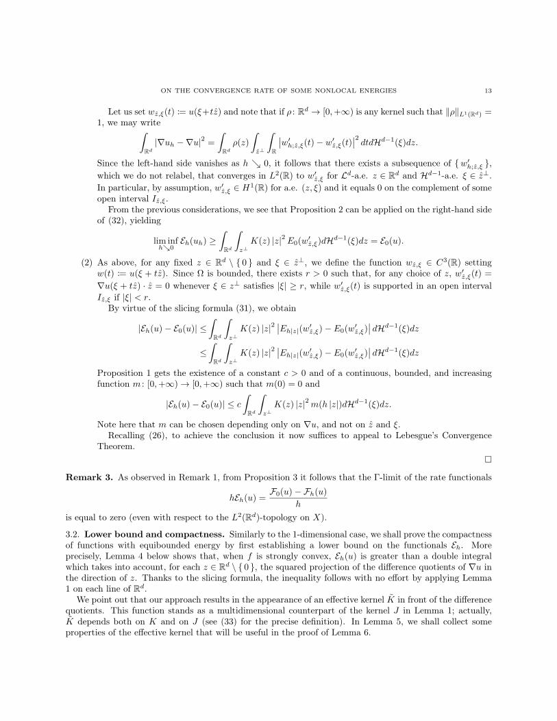
3.2. Lower bound and compactness. Similarly to the 1-dimensional case, we shall prove the compactnessof functions with equibounded energy by first establishing a lower bound on the functionals Eh. Moreprecisely, Lemma 4 below shows that, when f is strongly convex, Eh(u) is greater than a double integralwhich takes into account, for each z ∈ Rd \ 0 , the squared projection of the difference quotients of ∇u inthe direction of z. Thanks to the slicing formula, the inequality follows with no effort by applying Lemma1 on each line of Rd.
We point out that our approach results in the appearance of an effective kernel K in front of the differencequotients. This function stands as a multidimensional counterpart of the kernel J in Lemma 1; actually,K depends both on K and on J (see (33) for the precise definition). In Lemma 5, we shall collect someproperties of the effective kernel that will be useful in the proof of Lemma 6.
14 A. CHAMBOLLE, M. NOVAGA, AND V. PAGLIARI
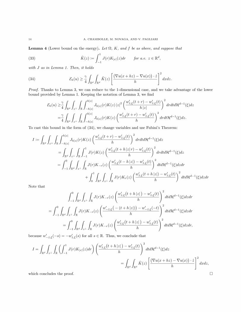
Lemma 4 (Lower bound on the energy). Let Ω, K, and f be as above, and suppose that
(33) K(z) :=
ˆ 1
−1
J(r)K|r|(z)dr for a.e. z ∈ Rd,
with J as in Lemma 1. Then, it holds
(34) Eh(u) ≥ γ
4
ˆRd
ˆRd
K(z)
[(∇u(x+ hz)−∇u(x)
)· z
h
]2
dxdz.
Proof. Thanks to Lemma 3, we can reduce to the 1-dimensional case, and we take advantage of the lowerbound provided by Lemma 1. Keeping the notation of Lemma 3, we find
Eh(u) ≥γ4
ˆRd
ˆz⊥
ˆR
ˆ h|z|
−h|z|Jh|z|(r)K(z) |z|2
(w′z,ξ(t+ r)− w′z,ξ(t)
h |z|
)2
drdtdHd−1(ξ)dz
=γ
4
ˆRd
ˆz⊥
ˆR
ˆ h|z|
−h|z|Jh|z|(r)K(z)
(w′z,ξ(t+ r)− w′z,ξ(t)
h
)2
drdtHd−1(ξ)dz.
To cast this bound in the form of (34), we change variables and use Fubini’s Theorem:
I :=
ˆRd
ˆz⊥
ˆR
ˆ h|z|
−h|z|Jh|z|(r)K(z)
(w′z,ξ(t+ r)− w′z,ξ(t)
h
)2
drdtdHd−1(ξ)dz
=
ˆRd
ˆz⊥
ˆR
ˆ 1
−1
J(r)K(z)
(w′z,ξ(t+ h |z| r)− w′z,ξ(t)
h
)2
drdtdHd−1(ξ)dz
=
ˆ 0
−1
ˆRd
ˆz⊥
ˆRJ(r)K−r(z)
(w′z,ξ(t− h |z|)− w′z,ξ(t)
h
)2
dtdHd−1(ξ)dzdr
+
ˆ 1
0
ˆRd
ˆz⊥
ˆRJ(r)Kr(z)
(w′z,ξ(t+ h |z|)− w′z,ξ(t)
h
)2
dtdHd−1(ξ)dzdr
Note thatˆ 0
−1
ˆRd
ˆz⊥
ˆRJ(r)K−r(z)
(w′z,ξ
(t+ h |z|
)− w′z,ξ(t)
h
)2
dtdHd−1(ξ)dzdr
=
ˆ 0
−1
ˆRd
ˆz⊥
ˆRJ(r)K−r(z)
(w′−z,ξ
(− (t+ h |z|)
)− w′−z,ξ(−t)
h
)2
dtdHd−1(ξ)dzdr
=
ˆ 0
−1
ˆRd
ˆz⊥
ˆRJ(r)K−r(z)
(w′z,ξ
(t+ h |z|
)− w′z,ξ(t)
h
)2
dtdHd−1(ξ)dzdr,
because w′−z,ξ(−s) = −w′z,ξ(s) for all s ∈ R. Thus, we conclude that
I =
ˆRd
ˆz⊥
ˆR
(ˆ 1
−1
J(r)K|r|(z)dr
)(w′z,ξ
(t+ h |z|
)− w′z,ξ(t)
h
)2
dtdHd−1(ξ)dz
=
ˆRd
ˆRd
K(z)
[(∇u(x+ hz)−∇u(x)
)· z
h
]2
dxdz,
which concludes the proof.
ON THE CONVERGENCE RATE OF SOME NONLOCAL ENERGIES 15
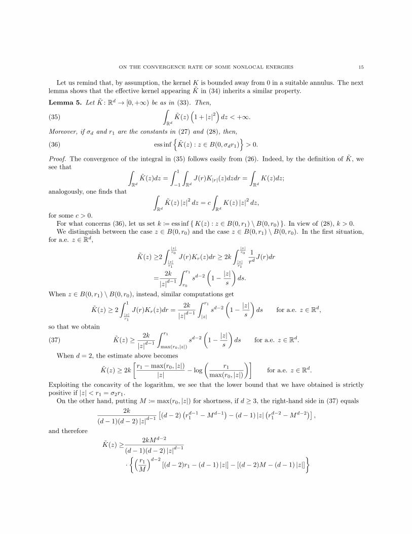
Let us remind that, by assumption, the kernel K is bounded away from 0 in a suitable annulus. The nextlemma shows that the effective kernel appearing K in (34) inherits a similar property.
Lemma 5. Let K : Rd → [0,+∞) be as in (33). Then,
(35)ˆRd
K(z)(
1 + |z|2)dz < +∞.
Moreover, if σd and r1 are the constants in (27) and (28), then,
(36) ess infK(z) : z ∈ B(0, σdr1)
> 0.
Proof. The convergence of the integral in (35) follows easily from (26). Indeed, by the definition of K, wesee that ˆ
Rd
K(z)dz =
ˆ 1
−1
ˆRd
J(r)K|r|(z)dzdr =
ˆRd
K(z)dz;
analogously, one finds that ˆRd
K(z) |z|2 dz = c
ˆRd
K(z) |z|2 dz,
for some c > 0.For what concerns (36), let us set k := ess inf K(z) : z ∈ B(0, r1) \B(0, r0) . In view of (28), k > 0.We distinguish between the case z ∈ B(0, r0) and the case z ∈ B(0, r1) \ B(0, r0). In the first situation,
for a.e. z ∈ Rd,
K(z) ≥2
ˆ |z|r0
|z|r1
J(r)Kr(z)dr ≥ 2k
ˆ |z|r0
|z|r1
1
rdJ(r)dr
=2k
|z|d−1
ˆ r1
r0
sd−2
(1− |z|
s
)ds.
When z ∈ B(0, r1) \B(0, r0), instead, similar computations get
K(z) ≥ 2
ˆ 1
|z|r1
J(r)Kr(z)dr =2k
|z|d−1
ˆ r1
|z|sd−2
(1− |z|
s
)ds for a.e. z ∈ Rd,
so that we obtain
(37) K(z) ≥ 2k
|z|d−1
ˆ r1
max(r0,|z|)sd−2
(1− |z|
s
)ds for a.e. z ∈ Rd.
When d = 2, the estimate above becomes
K(z) ≥ 2k
[r1 −max(r0, |z|)
|z|− log
(r1
max(r0, |z|)
)]for a.e. z ∈ Rd.
Exploiting the concavity of the logarithm, we see that the lower bound that we have obtained is strictlypositive if |z| < r1 = σ2r1.
On the other hand, putting M := max(r0, |z|) for shortness, if d ≥ 3, the right-hand side in (37) equals2k
(d− 1)(d− 2) |z|d−1
[(d− 2)
(rd−11 −Md−1
)− (d− 1) |z|
(rd−21 −Md−2
)],
and therefore
K(z) ≥ 2kMd−2
(d− 1)(d− 2) |z|d−1
·( r1
M
)d−2
[(d− 2)r1 − (d− 1) |z|]− [(d− 2)M − (d− 1) |z|]
16 A. CHAMBOLLE, M. NOVAGA, AND V. PAGLIARI
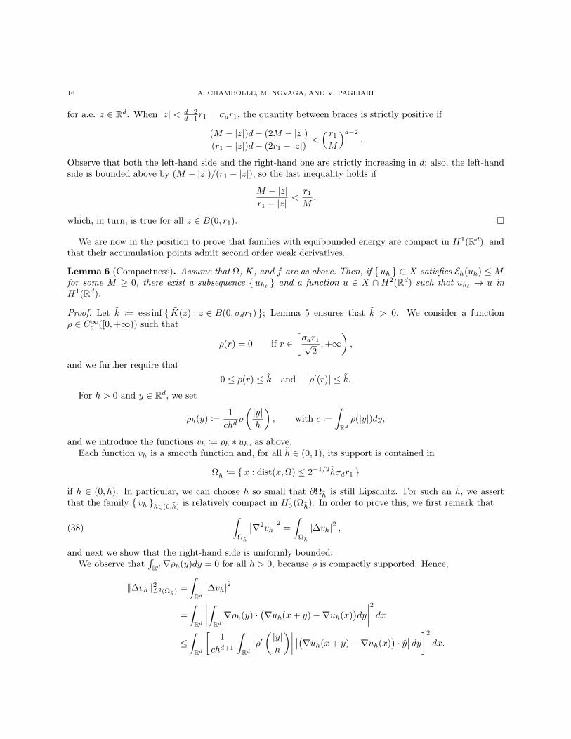
for a.e. z ∈ Rd. When |z| < d−2d−1r1 = σdr1, the quantity between braces is strictly positive if
(M − |z|)d− (2M − |z|)(r1 − |z|)d− (2r1 − |z|)
<( r1
M
)d−2
.
Observe that both the left-hand side and the right-hand one are strictly increasing in d; also, the left-handside is bounded above by (M − |z|)/(r1 − |z|), so the last inequality holds if
M − |z|r1 − |z|
<r1
M,
which, in turn, is true for all z ∈ B(0, r1).
We are now in the position to prove that families with equibounded energy are compact in H1(Rd), andthat their accumulation points admit second order weak derivatives.
Lemma 6 (Compactness). Assume that Ω, K, and f are as above. Then, if uh ⊂ X satisfies Eh(uh) ≤Mfor some M ≥ 0, there exist a subsequence uh`
and a function u ∈ X ∩ H2(Rd) such that uh`→ u in
H1(Rd).
Proof. Let k := ess inf K(z) : z ∈ B(0, σdr1) ; Lemma 5 ensures that k > 0. We consider a functionρ ∈ C∞c ([0,+∞)) such that
ρ(r) = 0 if r ∈[σdr1√
2,+∞
),
and we further require that0 ≤ ρ(r) ≤ k and |ρ′(r)| ≤ k.
For h > 0 and y ∈ Rd, we set
ρh(y) :=1
chdρ
(|y|h
), with c :=
ˆRd
ρ(|y|)dy,
and we introduce the functions vh := ρh ∗ uh, as above.Each function vh is a smooth function and, for all h ∈ (0, 1), its support is contained in
Ωh := x : dist(x,Ω) ≤ 2−1/2hσdr1
if h ∈ (0, h). In particular, we can choose h so small that ∂Ωh is still Lipschitz. For such an h, we assertthat the family vh h∈(0,h) is relatively compact in H1
0 (Ωh). In order to prove this, we first remark that
(38)ˆ
Ωh
∣∣∇2vh∣∣2 =
ˆΩh
|∆vh|2 ,
and next we show that the right-hand side is uniformly bounded.We observe that
´Rd ∇ρh(y)dy = 0 for all h > 0, because ρ is compactly supported. Hence,
‖∆vh‖2L2(Ωh) =
ˆRd
|∆vh|2
=
ˆRd
∣∣∣∣ˆRd
∇ρh(y) ·(∇uh(x+ y)−∇uh(x)
)dy
∣∣∣∣2 dx≤ˆRd
[1
chd+1
ˆRd
∣∣∣∣ρ′( |y|h)∣∣∣∣ ∣∣(∇uh(x+ y)−∇uh(x)
)· y∣∣ dy]2
dx.
ON THE CONVERGENCE RATE OF SOME NONLOCAL ENERGIES 17
By our choice of ρ and (36), we find
‖∆vh‖2L2(Ωh) ≤ˆRd
[1
ch
ˆRd
Kh(y)∣∣(∇uh(x+ y)−∇uh(x)
)· y∣∣ dy]2
dx
≤ˆRd
[1
ch
ˆRd
K(z)∣∣(∇uh(x+ hz)−∇uh(x)
)· z∣∣ dz]2
dx
Further, since K ∈ L1(Rd), Jensen’s inequality and Fubini’s Theorem yield
‖∆vh‖2L2(Ωh) ≤‖K‖L1(Rd)
c2
ˆRd
ˆRd
K(z)
[(∇uh(x+ hz)−∇uh(x)
)· z
h
]2
dxdz.
The lower bound (34) entails
‖∆vh‖2L2(Ωh) ≤4
c2γ‖K‖L1(Rd)Eh(uh),
so that, in view of the assumption Eh(uh) ≤M and of (38), we get
(39) ‖∇2vh‖2L2(Ωh) ≤4M
c2γ‖K‖L1(Rd).
We argue as in the proof of Lemma 2. We recall that, for h ∈ (0, h), each vh vanishes on the complementof Ωh, and thus, by Poincaré inequality, (39) implies a uniform bound on the norms ‖vh‖H2
0 (Ωh). As aconsequence, by Rellich-Kondrachov Theorem, the family vh h∈(0,h) of the restrictions of the functionsvh to Ωh admits a subsequence vh`
that converges in H10 (Ωh) to a function u ∈ H2
0 (Ωh). Actually, thesupport of u is contained in Ω, and, if we put,
u(x) :=
u(x) if x ∈ Ω,
0 otherwise,
we infer that vh` converges in H1(Rd) to u ∈ X ∩H2(Rd).
To accomplish the proof, it suffices to show that the L2 distance between ∇uh and ∇vh vanishes whenh 0. Since ρh has unit L1(Rd)-norm and it is radial, we have
ˆRd
|∇vh(x)−∇uh(x)|2dx =
ˆRd
∣∣∣∣ˆRd
ρh(y)(∇uh(x+ y)−∇uh(x)
)dy
∣∣∣∣2 dx≤1
4
ˆRd
∣∣∣∣ˆRd
ρh(y)(∇uh(x+ y) +∇uh(x− y)− 2∇uh(x)
)dy
∣∣∣∣2 dx≤1
4
ˆRd
ˆRd
ρh(y) |∇uh(x+ y) +∇uh(x− y)− 2∇uh(x)|2 dydx.
We remark that for any fixed y ∈ Rd \ 0 and for all p ∈ Rd, the identity |p|2 = |p · y|2 + |(Id− y ⊗ y)p|2can be reformulated as
|p|2 = |p · y|2 +
ˆy⊥π(|η|) |p · η|2 dHd−1(η)
= |p · y|2 +1
h2
ˆy⊥πh(η) |p · η|2 dHd−1(η),
(40)
where π : [0,+∞)→ [0,+∞) is a continuous function such thatˆe⊥d
π(|η|) |η|2 dHd−1(η) = 1,
18 A. CHAMBOLLE, M. NOVAGA, AND V. PAGLIARI
and πh(η) := h−d+1π(|η| /h). We further prescribe that
π(r) = 0 if r ∈[σdr1√
2,+∞
)and that limr0 η(r)/r ∈ R.
We apply the formula (40) to ph(x, y) := ∇uh(x+ y) +∇uh(x− y)− 2∇uh(x) and we find that
(41)ˆRd
|∇vh(x)−∇uh(x)|2 dx ≤ 1
4(I1 + I2) ,
whereI1 :=
ˆRd
ˆRd
ρh(y) |y|2 |ph(x, y) · y|2 dydx,
I2 :=1
h2
ˆRd
ˆRd
ˆy⊥ρh(y)πh(η) |ph(x, y) · η|2 dHd−1(η)dydx.
We first consider I1. Keeping in mind that ρ is compactly supported and ρ(|y|) ≤ k ≤ K(y) for a.e.y ∈ B(0, 2−1/2σdr1), we get
I1 ≤(σdr1)2
c
[ˆRd
ˆRd
Kh(y)∣∣(∇uh(x+ y)−∇uh(x)
)· y∣∣2 dydx
+
ˆRd
ˆRd
Kh(y)∣∣(∇uh(x− y)−∇uh(x)
)· y∣∣2 dydx] ,
and, by (34),
(42) I1 ≤8(σdr1)2M
cγh2.
As for I2, we assert that there exist a constant L > 0, depending on d, σd, r1, k, and c, such that
(43) I1 ≤LM
γh2.
To prove the claim, we write the integrand appearing in I2 as follows:
ph(x, y) · η =(∇uh(x+ y) +∇uh(x− y)− 2∇uh(x)
)· η
=(∇uh(x+ y) +∇uh(x− y)− 2∇uh(x− η)
)· η
+ 2(∇uh(x− η)−∇uh(x)
)· η
=(∇uh(x+ y)−∇uh(x− η)
)· (η + y)
+(∇uh(x− y)−∇uh(x− η)
)· (η − y)
−(∇uh(x+ y)−∇uh(x− y)
)· y + 2
(∇uh(x− η)−∇uh(x)
)· η.
We plug this identity in the definition of I2 and we find that
I2 ≤4
c
ˆRd
ˆRd
ˆy⊥ρ(|y|)π(|η|)
∣∣(∇uh(x+ hy)−∇uh(x− hη))· (η + y)
∣∣2 dHd−1(η)dydx
+4
c
ˆRd
ˆRd
ˆy⊥ρ(|y|)π(|η|)
∣∣(∇uh(x− hy)−∇uh(x− hη))· (η − y)
∣∣2 dHd−1(η)dydx
+8
c‖π‖L1(e⊥d )
ˆRd
ˆRd
ρ(|y|) |y|2∣∣(∇uh(x+ hy)−∇uh(x)
)· y∣∣2 dydx
+16
c
ˆRd
ˆRd
ˆy⊥ρ(|y|)π(|η|)
∣∣(∇uh(x+ hη)−∇uh(x))· η∣∣2 dHd−1(η)dydx.
ON THE CONVERGENCE RATE OF SOME NONLOCAL ENERGIES 19
We estimate separately each of the contributions on the right-hand side.Let us set Sd−1
+ := e ∈ Sd−1 : e · ed > 0 and Sd−1− := e ∈ Sd−1 : e · ed < 0 . Hereafter, we denote by L
any strictly positive constant depending only on d, σd, r1, and on the norms of ρ and π.Taking advantage of the Coarea Formula, we rewrite the first addendum as follows:
ˆRd
ˆRd
ˆy⊥ρ(|y|)π(|η|)
∣∣(∇uh(x+ hy)−∇uh(x− hη))· (η + y)
∣∣2 dHd−1(η)dydx
=
ˆRd
ˆRd
ˆy⊥ρ(|y|)π(|η|)
∣∣(∇uh(x+ h(η + y))−∇uh(x))· (η + y)
∣∣2 dHd−1(η)dxdy
=
ˆSd−1+
ˆRd
ˆR
ˆe⊥rd−1ρ(r)π(|η|)
∣∣(∇uh(x+ h(η + re))−∇uh(x))· (η + re)
∣∣2 dHd−1(η)drdxdHd−1(e)
=
ˆSd−1+
ˆRd
ˆRd
|y|2 |y · e|d−1ρ(|y · e|)π
(|(Id− e⊗ e)y|
) ∣∣(∇uh(x+ hy)−∇uh(x))· y∣∣2 dydxdHd−1(e).
Similarly, we have
ˆRd
ˆRd
ˆy⊥ρ(|y|)π(|η|)
∣∣(∇uh(x− hy)−∇uh(x− hη))· (η − y)
∣∣2 dHd−1(η)dydx
=
ˆSd−1−
ˆRd
ˆRd
|y|2 |y · e|d−1ρ(|y · e|)π
(|(Id− e⊗ e)y|
) ∣∣(∇uh(x+ hy)−∇uh(x))· y∣∣2 dydxdHd−1(e),
and thus
ˆRd
ˆRd
ˆy⊥ρ(|y|)π(|η|)
∣∣(∇uh(x+ hy)−∇uh(x− hη))· (η + y)
∣∣2 dHd−1(η)dydx
+
ˆRd
ˆRd
ˆy⊥ρ(|y|)π(|η|)
∣∣(∇uh(x− hy)−∇uh(x− hη))· (η − y)
∣∣2 dHd−1(η)dydx
=
ˆSd−1
ˆRd
ˆRd
|y · e|d−1 |y|2 ρ(|y · e|)π(|(Id− e⊗ e)y|
) ∣∣(∇uh(x+ hy)−∇uh(x))· y∣∣2 dydxdHd−1(e).
Let us recall that ρ(r) = η(r) = 0 if r /∈ [0, 2−1/2σdr1), whence, for any e ∈ Sd−1, the product ρ(|y · e|)π(|(Id− e⊗ e)y|
)vanishes outside the cylinder
Ce := y ∈ Rd : |y · e| , |(Id− e⊗ e)y| ∈ [0, 2−1/2σdr1) ⊂ B(0, σdr1).
We therefore see that the last multiple integral equals
ˆSd−1
ˆRd
ˆCe
|y · e|d−1 |y|2 ρ(|y · e|)π(|(Id− e⊗ e)y|
) ∣∣(∇uh(x+ hy)−∇uh(x))· y∣∣2 dydxdHd−1(e)
≤ LˆSd−1
ˆRd
ˆCe
K(y)∣∣(∇uh(x+ hy)−∇uh(x)
)· y∣∣2 dydxdHd−1(e)
≤ LM
γh2.

20 A. CHAMBOLLE, M. NOVAGA, AND V. PAGLIARI
We then obtain
(44)4
c
ˆRd
ˆRd
ˆy⊥ρ(|y|)π(|η|)
∣∣(∇uh(x+ hy)−∇uh(x− hη))· (η + y)
∣∣2 dHd−1(η)dydx
+4
c
ˆRd
ˆRd
ˆy⊥ρ(|y|)π(|η|)
∣∣(∇uh(x− hy)−∇uh(x− hη))· (η − y)
∣∣2 dHd−1(η)dydx
≤ LM
γh2.
Next, we have
(45)8
c‖π‖L1(e⊥d )
ˆRd
ˆRd
ρ(|y|) |y|2∣∣(∇uh(x+ hy)−∇uh(x)
)· y∣∣2 dydx ≤ LM
γh2,
(46)16
c
ˆRd
ˆRd
ˆy⊥ρ(|y|)π(|η|)
∣∣(∇uh(x+ hη)−∇uh(x))· η∣∣2 dHd−1(η)dydx ≤ LM
γh2.
The bound in (45) may be deduced as the one in (42), so, to establish (43), we are only left to prove (46).To this aim, let ψ ∈ C∞c (Rd × Rd) be a test function. By a standard argument and Fubini’s Theorem wehave that ˆ
Rd
ˆy⊥ρ(|y|)π(|η|)ψ(y, η)dHd−1(η)dy
= limε0
ˆRd
ˆRd
|y|2εχ t<ε (|η · y|)ρ(|y|)π(|η|)ψ(y, η)dηdy
= limε0
ˆRd
π(|η|)|η|
(ˆRd
|η|2εχ t<ε (|η · y|)ρ(|y|) |y|ψ(y, η)dy
)dη
=
ˆRd
ˆη⊥
π(|η|)|η|
ρ(|y|) |y|ψ(y, η)dHd−1(y)dη.
It follows that
Rd
ˆRd
ˆy⊥ρ(|y|)π(|η|)
∣∣(∇uh(x+ hη)−∇uh(x))· η∣∣2 dHd−1(η)dydx
=
ˆRd
ˆRd
ˆη⊥
π(|η|)|η|
ρ(|y|) |y|∣∣(∇uh(x+ hη)−∇uh(x)
)· η∣∣2 dHd−1(y)dηdx
≤LˆRd
ˆRd
K(η)∣∣(∇uh(x+ hη)−∇uh(x)
)· η∣∣2 dηdx
(recall that we assume limr0 η(r)/r to be finite). In view of the bound on the energy, we retrieve (46).In conclusion, from (41), (42), and (43), we obtainˆ
Rd
|∇vh(x)−∇uh(x)|2 dx ≤ LM
γh2,
as desired. This concludes the proof.
Remark 4. By choosing uh = u in Lemma 6 we obtain a criterion for an H1-function to belong to H2(Rd),namely a function u ∈ X is in H2(Rd) if and only if Eh(u) ≤M for some M > 0 and for all h small enough.
We can now conclude the proof of Theorem 2.
Proof of Theorem 2. The compactness result in statement (1) of Theorem 2 is contained in Lemma 6.The upper limit inequality (3) follows by Proposition 3 and a standard density argument, as in the
1-dimensional case.

ON THE CONVERGENCE RATE OF SOME NONLOCAL ENERGIES 21
As for the lower limit inequality (2), for any u ∈ X and for any family uh ⊂ X that converges to u inH1(Rd), we may focus on the situation when there exists M ≥ 0 such that |Eh(uh)| ≤ M for all h > 0. ByLemma 6, we have that u ∈ H2(Rd). Then, (2) follows by Proposition 3.
Remark 5. We conclude by noticing that the Γ-convergence result in Theorem 2, statements (2) and (3),still holds if we replace X with H1(Rd), with essentially the same proof. On the other hand, being Rdnon-compact, the compactness result in statement (1) of Theorem 2 does not hold in this case.
References
[1] G. Alberti and G. Bellettini, A non-local anisotropic model for phase transitions: asymptotic behaviourof rescaled energies, European Journal of Applied Mathematics 9 (1998), no. 3, 261–284.
[2] J. Berendsen and V. Pagliari, On the asymptotic behaviour of nonlocal perimeters, Preprint, to appearon ESAIM: COCV.
[3] J. Bourgain, H. Brezis, and P. Mironescu, Another look at Sobolev spaces, Optimal control and partialdifferential equations, IOS, Amsterdam, 2001, pp. 439–455.
[4] A. Braides, Γ-convergence for beginners, Oxford Lecture Series in Mathematics and its Applications,vol. 22, Oxford University Press, Oxford, 2002.
[5] A. Braides and L. Truskinovsky, Asymptotic expansions by Γ-convergence, Contin. Mech. Thermodyn.20 (2008), no. 1, 21–62, DOI 10.1007/s00161-008-0072-2.
[6] G. Dal Maso, An introduction to Γ-convergence, Progress in Nonlinear Differential Equations and theirApplications, vol. 8, Birkhäuser Boston, Inc., Boston, MA, 1993.
[7] M. Gobbino, Finite difference approximation of the Mumford-Shah functional, Comm. Pure Appl. Math.51 (1998), no. 2, 197–228.
[8] M. Gobbino and M. Mora, Finite-difference approximation of free-discontinuity problems, Proceedingsof the Royal Society of Edinburgh Section A: Mathematics 131 (2001), no. 3, 567–595.
[9] C.B. Muratov and T.M. Simon, A nonlocal isoperimetric problem with dipolar repulsion, Preprint, toappear on Commun. Math. Phys.
[10] M.A. Peletier, R. Planqué, and M. Röger, Sobolev regularity via the convergence rate of convolutionsand Jensen’s inequality, Ann. Sc. Norm. Super. Pisa Cl. Sci. (5) 6 (2007), no. 4, 499–510.
[11] A.C. Ponce, A new approach to Sobolev spaces and connections to Γ-convergence, Calc. Var. PartialDifferential Equations 19 (2004), no. 3, 229–255.
(A. Chambolle) CMAP, Ecole Polytechnique, 91128 Palaiseau Cedex, France. Email: [email protected].
(M. Novaga, V. Pagliari) Dipartimento di Matematica, Università di Pisa, Largo B. Pontecorvo 5, 56127 Pisa,Italy. Email: [email protected], [email protected].