The Fractional Laplacian for the Fractional PDEsI

Kailai Xu1

AbstractRecent years have witnessed a notable boom in the research interest in the modeling usingnonlocal operators. The fractional Laplacian, which is the generator of a symmetric α-stableprocess, has been used for modeling lossy media, option price, turbulence, etc. However,it is still not clear how the fractional Laplacian should be defined for the bounded domainmodeling. This note has two objectives: the first is to derive the fractional PDEs from theprobability view of the fractional Laplacian; the second is to define Dirichlet-type boundaryconditions based on this interpretation. It serves as a clarification of the current confusionover the fractional PDE modeling via the fractional Laplacian.

Keywords: fractional PDE, fractional Laplacian, symmetric α-stable process

IUpdated on May 9, 2018.Email address: kailaix@stanford.edu (Kailai Xu)

Contents

1 Introduction 3

2 Stochastic Process and the Fractional Laplacian 32.1 Lévy Process . . . . . . . . . . . . . . . . . . . . . . . . . . . . . . . . . . . 32.2 Special Case: Symmetric α-stable Process . . . . . . . . . . . . . . . . . . . 52.3 Stochastic Differential Equations Driven by Levy Process . . . . . . . . . . . 72.4 Connection with the fractional Laplacian . . . . . . . . . . . . . . . . . . . . 82.5 Feynman-Kac Representation . . . . . . . . . . . . . . . . . . . . . . . . . . 92.6 Generation of the Symmetric α-stable Distribution . . . . . . . . . . . . . . 102.7 Generation of the Symmetric α-stable Process . . . . . . . . . . . . . . . . . 12

3 The Fractional Laplacian in the Bounded Domain 123.1 Definition of the Fractional Laplacian on the Bounded Domain . . . . . . . . 123.2 Integration By Parts . . . . . . . . . . . . . . . . . . . . . . . . . . . . . . . 14

4 Fractional PDE in Rd 154.1 Fractional Diffusion Equation . . . . . . . . . . . . . . . . . . . . . . . . . . 164.2 Fractional Advection-diffusion Equation . . . . . . . . . . . . . . . . . . . . . 184.3 Fokker-Planck Equation . . . . . . . . . . . . . . . . . . . . . . . . . . . . . 19

5 Fractional PDE in the Bounded Domain 205.1 The Fractional Poisson Problem . . . . . . . . . . . . . . . . . . . . . . . . . 205.2 Fractional PDEs in the Bounded Domain . . . . . . . . . . . . . . . . . . . . 215.3 Remarks on 1D Case . . . . . . . . . . . . . . . . . . . . . . . . . . . . . . . 21

6 Conclusion 22

7 References 22

1. Introduction

The fractional PDEs have attracted considerable attention recently due to its applicationin soft matter [1], elasticity [2], turbulence [3], anomalous diffusion [4], finance [5], imagedenoising [6], porous media flow [7], etc. Among different fractional operators, the fractionalLaplacian has been intensively studied in the recent literature. For example, [8] uses thefractional Laplacian for linear and nonlinear lossy media. [9] uses the fractional Laplacianfor option pricing in jump diffusion and exponential Lévy models. Recently, [10] providesthe first ever derivation of the fractional Laplacian operator as a means to represent themean friction in the turbulence modeling. For more application examples, see [11].

In this note, we consider the fractional Laplacian

(−∆)α/2u(x) := cα,dP.V.

∫R2

u(x)− u(y)

|x− y|d+αdy

where P.V. stands for the Cauchy principal value integration and

cα,d =2αΓ

(d+α2

)πd/2

∣∣Γ (−α2

)∣∣Over the years, researchers have investigated the fractional Laplacian from many perspec-

tives such as the probabilistic view, the potential theory or the PDEs. Different views leadto various definitions for the fractional Laplacian in Rd, which, under certain assumptions,are shown to be equivalent [12].

However, the community has not reached an agreement on how the fractional Laplacianshould be defined on a bounded domain, which is crucial for physical modeling. There aremainly three definitions in the literature: the restricted fractional Laplacian, the spectralfractional Laplacian, and the regional Laplacian. The definitions and discussions will becarried out as we proceed through the notes.

A main application of the fractional Laplacian is PDE modeling via the fractional Lapla-cian. The derivations of nonlocal models via the fractional Laplacian are very similar to thatof the classical models via the typical Laplacian such as the diffusion equation, except thatwe replace the underlying Gaussian process by its counterpart of the symmetric α-stable (orLévy) process. The derivation in this note assumes no advanced knowledge of probabilitytheory and will be self-contained.

2. Stochastic Process and the Fractional Laplacian

2.1. Lévy ProcessThroughout this note, (Ω,F ,F, P ) is a filtered probability space with filtration F =

Ft, t ≥ 0. We first define the Levy process L = Lt, t ≥ 0 with value in Rd and definedon (Ω,F ,F, P ).

Lévy process can be defined through some fundamental characterizations of its properties.

Definition 1 (Lévy process [13]). Let Lt, t ∈ [0,∞) be a stochastic process Xt : Ω → Rd

satisfyingL0 = 0, a.s.

stationary increments Lt − Ls ∼ Xt−s −X0 ∀s ≤ t

independent increments Lt − Ls⊥σ(Xr, r ≤ s) ∀s ≤ t

continuity in probability limt→0

P(|Xt −X0| > ε) = 0 ∀ε > 0

where ∼ stands for ‘same distribution’, ‘⊥’ stands for stochastic independence, σ(·) standsfor the sigma algebra.

Then L = Lt, t ≥ 0 is called Lévy process.We see that Levy process shares many similar properties with the Brownian motion. As

we will see, the Brownian motion is merely a special case of Levy process. The full extentto which we can characterize Lévy process is to describe its characteristic function, knownas Lévy-Khintchine formulaTheorem 1 (Lévy-Khintchine formula). Let Lt, t ≥ 0 be a Lévy process, then the charac-teristic function of the probability law at time t is

Eeiu·Lt = exp

(t

(iγ · u− 1

2∥σ · u∥2 +

∫Rd

(eiu·x − 1− iu · x1|x|<1

)ν(dx)

))(1)

where γ ∈ Rd, σσT ⪰ 0 and ν is a measure concentrated on Rd\0 satisfying∫Rd

(1 ∧ |x|2)ν(dx) < ∞ (2)

The tuple (γ, σ, ν) is called the characteristic triplet, where σσT is the covariance ma-trix. There exists a one-to-one correspondence between every Lévy process and the Lévytriple [14]. The first two parts in eq. (1) corresponds to a Gaussian process while the thirdcorresponds to a jump part; these two processes are independent.

There are two special cases of Levy process:• Poisson process, where the probability distribution pλ(k) = e−λλk

k!is concentrated

on k = 0, 1, 2, . . . for some λ > 0, then the corresponding Lévy tuple is (0, 0, λδ1).

• Gaussian process. Assume that the process have the linear drift µ and covarianceσσT , then the Lévy tuple is (µ, σ, 0).

We can reorganize the exponential in eq. (1) into term terms

t

(−iγ · u+

1

2∥σ · u∥2 −

∫Rd

(eiu·x − 1− iu · x1|x|<1

)ν(dx)

)= t

(−iγ · u+

1

2σσT |u|2

)− ν(|x| > 1)

∫|x|>1

(eiu·x − 1

) ν(dx)

ν(|x| > 1)

−∫|x|≤1

(eiu·x − 1− iux

)ν(dx) (3)

Actually, this decomposition leads to a remarkable decomposition of Lévy process

Theorem 2 (Lévy-Itô decomposition). Assume µ satisfies eq. (2), then there exists a proba-bility space on which three independent Lévy process exists: X(1) is a Gaussian process; X(2)

is a compound Poisson process; X(3) is a square integrable martingale. The characteristicexponents are given by eq. (3) respectively. Then X = X(1) +X(2) +X(3) is a Lévy processwith characteristic exponent given by eq. (3).

We can also decompose the Lévy process into

Xt = µdt+ σdWt + dJt (4)

where there is a one-to-one correspondence between the terms in eq. (4) and eq. (1). Dueto the uniqueness of the Lévy triple, such a decomposition is also unique.

2.2. Special Case: Symmetric α-stable ProcessThe symmetric α-stable process is the basic tool to understand the fractional Laplacian

as the generator of a stochastic process. The symmetric α-stable process can be definedthrough its Lévy-Khintchine representation

Eeiu·Xt = exp(−tγα|u|α), α ∈ (0, 2] (5)

where the dispersion γ represents the spread of the distribution. Symmetric α-stable processhas the scaling property cXc−αt ∼ Xt. Some authors will also include a drift term in eq. (5)

Eeiu·Xt = exp(t(µ · u− γα|u|α)), α ∈ (0, 2]

in this case, the distribution is symmetric around µ, which is the mean of the distributionfor 1 < α ≤ 2 and median for 0 < α ≤ 1.

Proposition 1. Let the levy measure be

ν(dx) =Cdx

|x|α+d(6)

then the Levy process with the triplets (0, 0, ν) is a symmetric α-stable process with charac-teristic function

exp

(− tC

cα,d|u|α

)Proof. Let Lt be the Lévy process with the triplets (0, 0, µ), then we have

Eeiu·Lt = exp

(Ct

∫Rd

(eiu·x − 1− iu · x1|x|<1

) dx

|x|α+d

)Let

g(u) :=

∫Rd

(eiu·x − 1− iu · x1|x|<1

) dx

|x|α+d

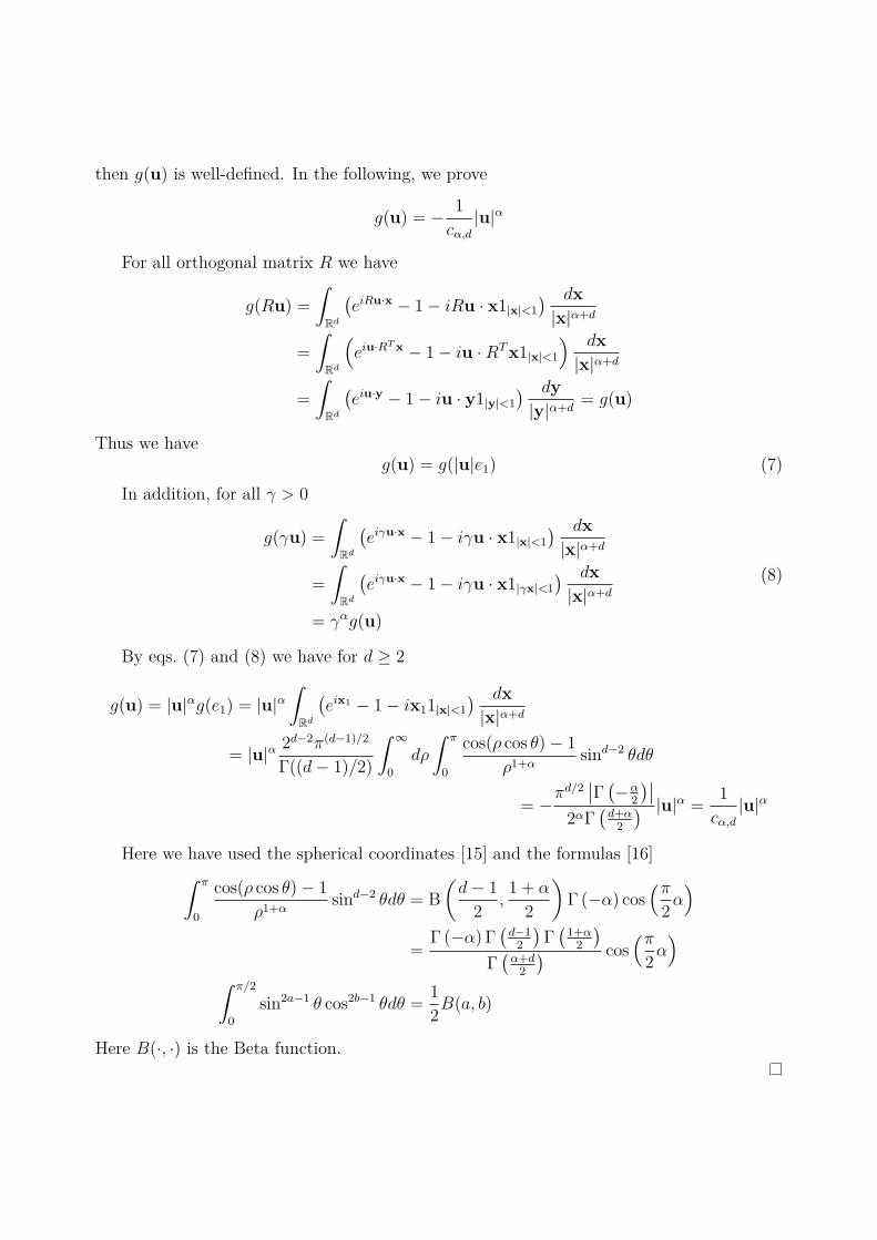
then g(u) is well-defined. In the following, we prove

g(u) = − 1

cα,d|u|α

For all orthogonal matrix R we have

g(Ru) =

∫Rd

(eiRu·x − 1− iRu · x1|x|<1

) dx

|x|α+d

=

∫Rd

(eiu·R

Tx − 1− iu ·RTx1|x|<1

) dx

|x|α+d

=

∫Rd

(eiu·y − 1− iu · y1|y|<1

) dy

|y|α+d= g(u)

Thus we haveg(u) = g(|u|e1) (7)

In addition, for all γ > 0

g(γu) =

∫Rd

(eiγu·x − 1− iγu · x1|x|<1

) dx

|x|α+d

=

∫Rd

(eiγu·x − 1− iγu · x1|γx|<1

) dx

|x|α+d

= γαg(u)

(8)

By eqs. (7) and (8) we have for d ≥ 2

g(u) = |u|αg(e1) = |u|α∫Rd

(eix1 − 1− ix11|x|<1

) dx

|x|α+d

= |u|α 2d−2π(d−1)/2

Γ((d− 1)/2)

∫ ∞

0

dρ

∫ π

0

cos(ρ cos θ)− 1

ρ1+αsind−2 θdθ

= −πd/2

∣∣Γ (−α2

)∣∣2αΓ

(d+α2

) |u|α =1

cα,d|u|α

Here we have used the spherical coordinates [15] and the formulas [16]∫ π

0

cos(ρ cos θ)− 1

ρ1+αsind−2 θdθ = B

(d− 1

2,1 + α

2

)Γ (−α) cos

(π2α)

=Γ (−α) Γ

(d−12

)Γ(1+α2

)Γ(α+d2

) cos(π2α)

∫ π/2

0

sin2a−1 θ cos2b−1 θdθ =1

2B(a, b)

Here B(·, ·) is the Beta function.

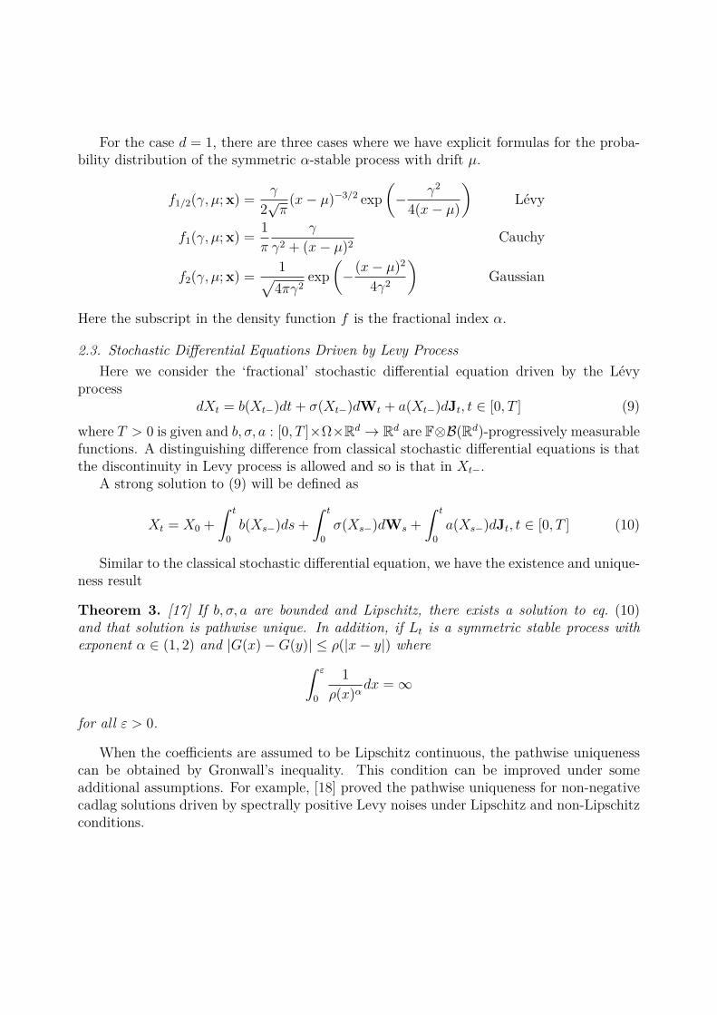
For the case d = 1, there are three cases where we have explicit formulas for the proba-bility distribution of the symmetric α-stable process with drift µ.

f1/2(γ, µ;x) =γ

2√π(x− µ)−3/2 exp

(− γ2

4(x− µ)

)Lévy

f1(γ, µ;x) =1

π

γ

γ2 + (x− µ)2Cauchy

f2(γ, µ;x) =1√4πγ2

exp

(−(x− µ)2

4γ2

)Gaussian

Here the subscript in the density function f is the fractional index α.

2.3. Stochastic Differential Equations Driven by Levy ProcessHere we consider the ‘fractional’ stochastic differential equation driven by the Lévy

processdXt = b(Xt−)dt+ σ(Xt−)dWt + a(Xt−)dJt, t ∈ [0, T ] (9)

where T > 0 is given and b, σ, a : [0, T ]×Ω×Rd → Rd are F⊗B(Rd)-progressively measurablefunctions. A distinguishing difference from classical stochastic differential equations is thatthe discontinuity in Levy process is allowed and so is that in Xt−.

A strong solution to (9) will be defined as

Xt = X0 +

∫ t

0

b(Xs−)ds+

∫ t

0

σ(Xs−)dWs +

∫ t

0

a(Xs−)dJt, t ∈ [0, T ] (10)

Similar to the classical stochastic differential equation, we have the existence and unique-ness result

Theorem 3. [17] If b, σ, a are bounded and Lipschitz, there exists a solution to eq. (10)and that solution is pathwise unique. In addition, if Lt is a symmetric stable process withexponent α ∈ (1, 2) and |G(x)−G(y)| ≤ ρ(|x− y|) where∫ ε

0

1

ρ(x)αdx = ∞

for all ε > 0.

When the coefficients are assumed to be Lipschitz continuous, the pathwise uniquenesscan be obtained by Gronwall’s inequality. This condition can be improved under someadditional assumptions. For example, [18] proved the pathwise uniqueness for non-negativecadlag solutions driven by spectrally positive Levy noises under Lipschitz and non-Lipschitzconditions.

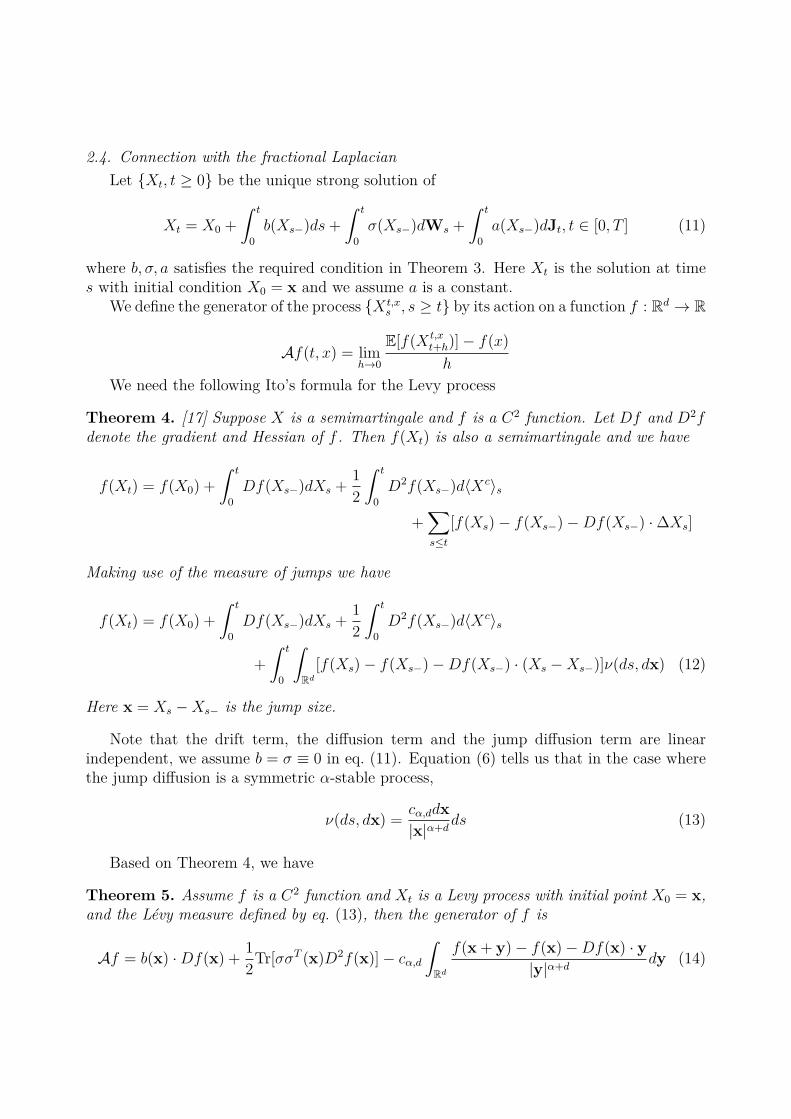
2.4. Connection with the fractional LaplacianLet Xt, t ≥ 0 be the unique strong solution of

Xt = X0 +

∫ t

0

b(Xs−)ds+

∫ t

0

σ(Xs−)dWs +

∫ t

0

a(Xs−)dJt, t ∈ [0, T ] (11)

where b, σ, a satisfies the required condition in Theorem 3. Here Xt is the solution at times with initial condition X0 = x and we assume a is a constant.

We define the generator of the process X t,xs , s ≥ t by its action on a function f : Rd → R

Af(t, x) = limh→0

E[f(X t,xt+h)]− f(x)

h

We need the following Ito’s formula for the Levy process

Theorem 4. [17] Suppose X is a semimartingale and f is a C2 function. Let Df and D2fdenote the gradient and Hessian of f . Then f(Xt) is also a semimartingale and we have

f(Xt) = f(X0) +

∫ t

0

Df(Xs−)dXs +1

2

∫ t

0

D2f(Xs−)d⟨Xc⟩s

+∑s≤t

[f(Xs)− f(Xs−)−Df(Xs−) ·∆Xs]

Making use of the measure of jumps we have

f(Xt) = f(X0) +

∫ t

0

Df(Xs−)dXs +1

2

∫ t

0

D2f(Xs−)d⟨Xc⟩s

+

∫ t

0

∫Rd

[f(Xs)− f(Xs−)−Df(Xs−) · (Xs −Xs−)]ν(ds, dx) (12)

Here x = Xs −Xs− is the jump size.

Note that the drift term, the diffusion term and the jump diffusion term are linearindependent, we assume b = σ ≡ 0 in eq. (11). Equation (6) tells us that in the case wherethe jump diffusion is a symmetric α-stable process,

ν(ds, dx) =cα,ddx

|x|α+dds (13)

Based on Theorem 4, we have

Theorem 5. Assume f is a C2 function and Xt is a Levy process with initial point X0 = x,and the Lévy measure defined by eq. (13), then the generator of f is

Af = b(x) ·Df(x) +1

2Tr[σσT (x)D2f(x)]− cα,d

∫Rd

f(x+ y)− f(x)−Df(x) · y|y|α+d

dy (14)

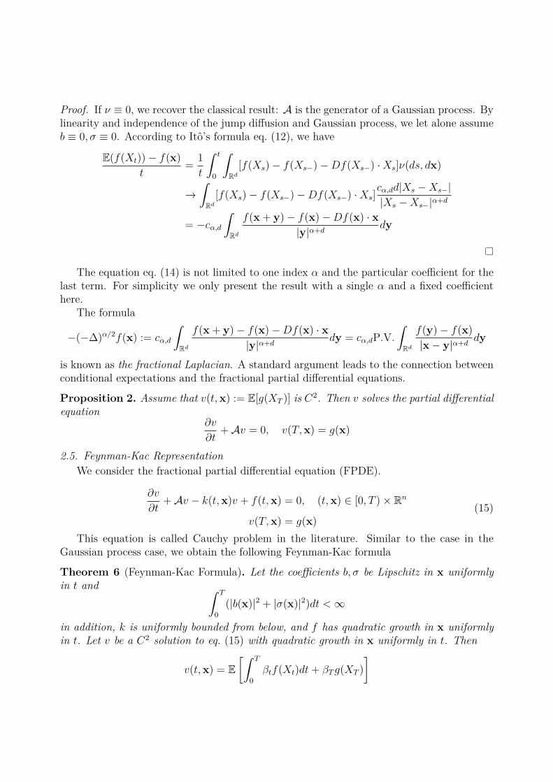
Proof. If ν ≡ 0, we recover the classical result: A is the generator of a Gaussian process. Bylinearity and independence of the jump diffusion and Gaussian process, we let alone assumeb ≡ 0, σ ≡ 0. According to Itô’s formula eq. (12), we have

E(f(Xt))− f(x)

t=

1

t

∫ t

0

∫Rd

[f(Xs)− f(Xs−)−Df(Xs−) ·Xs]ν(ds, dx)

→∫Rd

[f(Xs)− f(Xs−)−Df(Xs−) ·Xs]cα,dd|Xs −Xs−||Xs −Xs−|α+d

= −cα,d

∫Rd

f(x+ y)− f(x)−Df(x) · x|y|α+d

dy

The equation eq. (14) is not limited to one index α and the particular coefficient for thelast term. For simplicity we only present the result with a single α and a fixed coefficienthere.

The formula

−(−∆)α/2f(x) := cα,d

∫Rd

f(x+ y)− f(x)−Df(x) · x|y|α+d

dy = cα,dP.V.

∫Rd

f(y)− f(x)

|x− y|α+ddy

is known as the fractional Laplacian. A standard argument leads to the connection betweenconditional expectations and the fractional partial differential equations.

Proposition 2. Assume that v(t,x) := E[g(XT )] is C2. Then v solves the partial differentialequation

∂v

∂t+Av = 0, v(T,x) = g(x)

2.5. Feynman-Kac RepresentationWe consider the fractional partial differential equation (FPDE).

∂v

∂t+Av − k(t,x)v + f(t,x) = 0, (t,x) ∈ [0, T )× Rn

v(T,x) = g(x)(15)

This equation is called Cauchy problem in the literature. Similar to the case in theGaussian process case, we obtain the following Feynman-Kac formula

Theorem 6 (Feynman-Kac Formula). Let the coefficients b, σ be Lipschitz in x uniformlyin t and ∫ T

0

(|b(x)|2 + |σ(x)|2)dt < ∞

in addition, k is uniformly bounded from below, and f has quadratic growth in x uniformlyin t. Let v be a C2 solution to eq. (15) with quadratic growth in x uniformly in t. Then

v(t,x) = E[∫ T

0

βtf(Xt)dt+ βTg(XT )

]

where βt = exp(−∫ t

0k(Xu)du

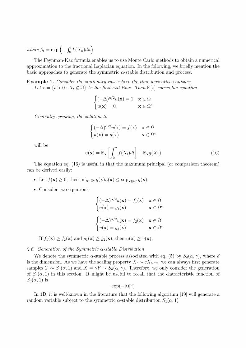
)The Feynman-Kac formula enables us to use Monte Carlo methods to obtain a numerical

approximation to the fractional Laplacian equation. In the following, we briefly mention thebasic approaches to generate the symmetric α-stable distribution and process.

Example 1. Consider the stationary case where the time derivative vanishes.Let τ = t > 0 : Xt ∈ Ω be the first exit time. Then E[τ ] solves the equation

(−∆)α/2u(x) = 1 x ∈ Ω

u(x) = 0 x ∈ Ωc

Generally speaking, the solution to(−∆)α/2u(x) = f(x) x ∈ Ω

u(x) = g(x) x ∈ Ωc

will beu(x) = Ex

[∫ τ

0

f(Xt)dt

]+ Exg(Xτ ) (16)

The equation eq. (16) is useful in that the maximum principal (or comparison theorem)can be derived easily:

• Let f(x) ≥ 0, then infx∈Ωc g(x)u(x) ≤ supx∈Ωc g(x).

• Consider two equations (−∆)α/2u(x) = f1(x) x ∈ Ω

u(x) = g1(x) x ∈ Ωc

(−∆)α/2v(x) = f2(x) x ∈ Ω

v(x) = g2(x) x ∈ Ωc

If f1(x) ≥ f2(x) and g1(x) ≥ g2(x), then u(x) ≥ v(x).

2.6. Generation of the Symmetric α-stable DistributionWe denote the symmetric α-stable process associated with eq. (5) by Sd(α, γ), where d

is the dimension. As we have the scaling property Xt ∼ cXtc−α , we can always first generatesamples Y ∼ Sd(α, 1) and X = γY ∼ Sd(α, γ). Therefore, we only consider the generationof Sd(α, 1) in this section. It might be useful to recall that the characteristic function ofSd(α, 1) is

exp(−|u|α)In 1D, it is well-known in the literature that the following algorithm [19] will generate a

random variable subject to the symmetric α-stable distribution S1(α, 1)

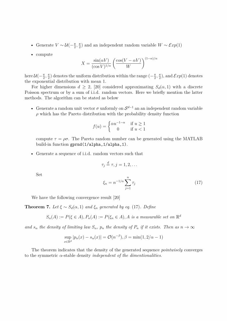
• Generate V ∼ U(−π2, π2) and an independent random variable W ∼ Exp(1)

• compute

X =sin(αV )

(cosV )1/α

(cos(V − αV )

W

)(1−α)/α

here U(−π2, π2) denotes the uniform distribution within the range (−π

2, π2), and Exp(1) denotes

the exponential distribution with mean 1.For higher dimensions d ≥ 2, [20] considered approximating Sd(α, 1) with a discrete

Poisson spectrum or by a sum of i.i.d. random vectors. Here we briefly mention the lattermethods. The algorithm can be stated as below

• Generate a random unit vector σ unformly on Sd−1 an an independent random variableρ which has the Pareto distribution with the probability density function

f(u) =

αu−1−α if u ≥ 1

0 if u < 1

compute τ = ρσ. The Pareto random number can be generated using the MATLABbuild-in function gprnd(1/alpha,1/alpha,1).

• Generate a sequence of i.i.d. random vectors such that

τjd= τ, j = 1, 2, . . .

Set

ξn = n−1/α

n∑j=1

τj (17)

We have the following convergence result [20]

Theorem 7. Let ξ ∼ Sd(α, 1) and ξn generated by eq. (17). Define

Sα(A) := P (ξ ∈ A), Pn(A) := P (ξn ∈ A), A is a measurable set on Rd

and sα the density of limiting law Sα, pn the density of Pn if it exists. Then as n → ∞

supx∈Rd

|pn(x)− sα(x)| = O(n−β), β = min(1, 2/α− 1)

The theorem indicates that the density of the generated sequence pointwisely convergesto the symmetric α-stable density independent of the dimentionalities.

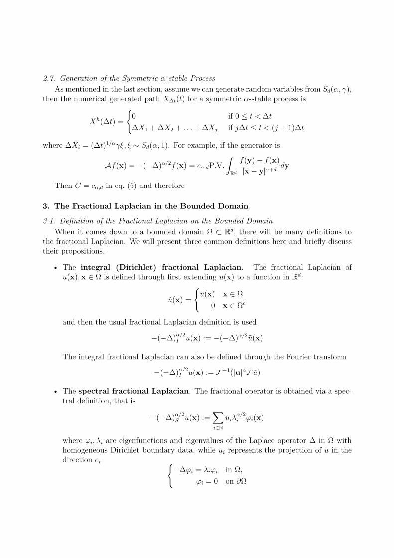
2.7. Generation of the Symmetric α-stable ProcessAs mentioned in the last section, assume we can generate random variables from Sd(α, γ),

then the numerical generated path X∆t(t) for a symmetric α-stable process is

Xh(∆t) =

0 if 0 ≤ t < ∆t

∆X1 +∆X2 + . . .+∆Xj if j∆t ≤ t < (j + 1)∆t

where ∆Xi = (∆t)1/αγξ, ξ ∼ Sd(α, 1). For example, if the generator is

Af(x) = −(−∆)α/2f(x) = cα,dP.V.

∫Rd

f(y)− f(x)

|x− y|α+ddy

Then C = cα,d in eq. (6) and therefore

3. The Fractional Laplacian in the Bounded Domain

3.1. Definition of the Fractional Laplacian on the Bounded DomainWhen it comes down to a bounded domain Ω ⊂ Rd, there will be many definitions to

the fractional Laplacian. We will present three common definitions here and briefly discusstheir propositions.

• The integral (Dirichlet) fractional Laplacian. The fractional Laplacian ofu(x),x ∈ Ω is defined through first extending u(x) to a function in Rd:

u(x) =

u(x) x ∈ Ω

0 x ∈ Ωc

and then the usual fractional Laplacian definition is used

−(−∆)α/2I u(x) := −(−∆)α/2u(x)

The integral fractional Laplacian can also be defined through the Fourier transform

−(−∆)α/2I u(x) := F−1(|u|αF u)

• The spectral fractional Laplacian. The fractional operator is obtained via a spec-tral definition, that is

−(−∆)α/2S u(x) :=

∑i∈N

uiλα/2i φi(x)

where φi, λi are eigenfunctions and eigenvalues of the Laplace operator ∆ in Ω withhomogeneous Dirichlet boundary data, while ui represents the projection of u in thedirection ei

−∆φi = λiφi in Ω,

φi = 0 on ∂Ω

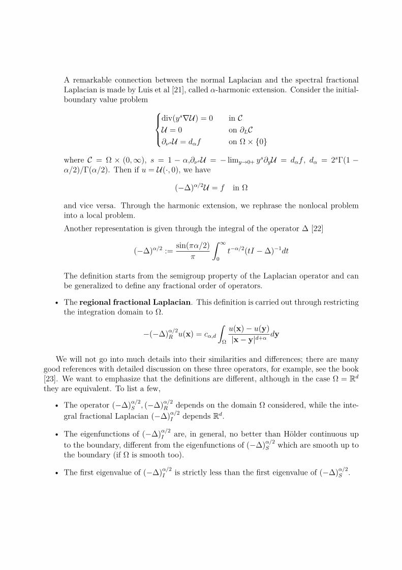
A remarkable connection between the normal Laplacian and the spectral fractionalLaplacian is made by Luis et al [21], called α-harmonic extension. Consider the initial-boundary value problem

div(ys∇U) = 0 in CU = 0 on ∂LC∂νsU = dαf on Ω× 0

where C = Ω × (0,∞), s = 1 − α,∂νsU = − limy→0+ ys∂yU = dαf , dα = 2sΓ(1 −α/2)/Γ(α/2). Then if u = U(·, 0), we have

(−∆)α/2U = f in Ω

and vice versa. Through the harmonic extension, we rephrase the nonlocal probleminto a local problem.Another representation is given through the integral of the operator ∆ [22]

(−∆)α/2 :=sin(πα/2)

π

∫ ∞

0

t−α/2(tI −∆)−1dt

The definition starts from the semigroup property of the Laplacian operator and canbe generalized to define any fractional order of operators.

• The regional fractional Laplacian. This definition is carried out through restrictingthe integration domain to Ω.

−(−∆)α/2R u(x) = cα,d

∫Ω

u(x)− u(y)

|x− y|d+αdy

We will not go into much details into their similarities and differences; there are manygood references with detailed discussion on these three operators, for example, see the book[23]. We want to emphasize that the definitions are different, although in the case Ω = Rd

they are equivalent. To list a few,

• The operator (−∆)α/2S , (−∆)

α/2R depends on the domain Ω considered, while the inte-

gral fractional Laplacian (−∆)α/2I depends Rd.

• The eigenfunctions of (−∆)α/2I are, in general, no better than Hölder continuous up

to the boundary, different from the eigenfunctions of (−∆)α/2S which are smooth up to

the boundary (if Ω is smooth too).

• The first eigenvalue of (−∆)α/2I is strictly less than the first eigenvalue of (−∆)

α/2S .

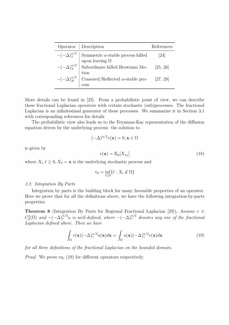
Operator Description References

−(−∆)α/2I Symmetric α-stable process killed

upon leaving Ω[24]

−(−∆)α/2S Subordinate killed Brownian Mo-

tion[25, 26]

−(−∆)α/2R Censored/Reflected α-stable pro-

cess[27, 28]

More details can be found in [23]. From a probabilistic point of view, we can describethese fractional Laplacian operators with certain stochastic (sub)processes. The fractionalLaplacian is an infinitesimal generator of these processes. We summarize it in Section 3.1with corresponding references for details

The probabilistic view also leads us to the Feynman-Kac representation of the diffusionequation driven by the underlying process: the solution to

(−∆)α/2v(x) = 0,x ∈ Ω

is given byv(x) = Ex[XτΩ ] (18)

where Xt, t ≥ 0, X0 = x is the underlying stochastic process and

τΩ = inft≥0

t : Xt ∈ Ω

3.2. Integration By PartsIntegration by parts is the building block for many favorable properties of an operator.

Here we prove that for all the definitions above, we have the following integration-by-partsproperties.

Theorem 8 (Integration By Parts for Regional Fractional Laplacian [29]). Assume v ∈C2

0(Ω) and −(−∆)α/2∗ u is well-defined, where −(−∆)

α/2∗ denotes any one of the fractional

Laplacian defined above. Then we have∫Ω

v(x)(−∆)α/2∗ u(x)dx =

∫Ω

u(x)(−∆)α/2∗ v(x)dx (19)

for all three definitions of the fractional Laplacian on the bounded domain.

Proof. We prove eq. (19) for different operators respectively.

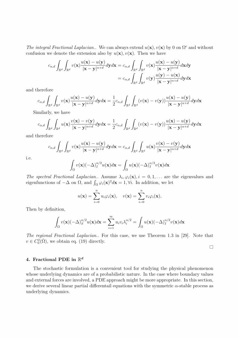
The integral Fractional Laplacian.. We can always extend u(x), v(x) by 0 on Ωc and withoutconfusion we denote the extension also by u(x), v(x). Then we have

cα,d

∫Rd

∫Rd

v(x)u(x)− u(y)

|x− y|α+ddydx = cα,d

∫Rd

∫Rd

v(x)u(x)− u(y)

|x− y|α+ddxdy

= cα,d

∫Rd

∫Rd

v(y)u(y)− u(x)

|x− y|α+ddydx

and therefore

cα,d

∫Rd

∫Rd

v(x)u(x)− u(y)

|x− y|α+ddydx =

1

2cα,d

∫Rd

∫Rd

(v(x)− v(y))u(x)− u(y)

|x− y|α+ddydx

Similarly, we have

cα,d

∫Rd

∫Rd

u(x)v(x)− v(y)

|x− y|α+ddydx =

1

2cα,d

∫Rd

∫Rd

(v(x)− v(y))u(x)− u(y)

|x− y|α+ddydx

and therefore

cα,d

∫Rd

∫Rd

v(x)u(x)− u(y)

|x− y|α+ddydx = cα,d

∫Rd

∫Rd

u(x)v(x)− v(y)

|x− y|α+ddydx

i.e. ∫Ω

v(x)(−∆)α/2I u(x)dx =

∫Ω

u(x)(−∆)α/2I v(x)dx

The spectral Fractional Laplacian.. Assume λi, φi(x), i = 0, 1, . . . are the eigenvalues andeigenfunctions of −∆ on Ω, and

∫Ωφi(x)

2dx = 1,∀i. In addition, we let

u(x) =n∑

i=0

uiφi(x), v(x) =n∑

i=0

viφi(x),

Then by definition,∫Ω

v(x)(−∆)α/2S u(x)dx =

∞∑i=1

uiviλα/2i =

∫Ω

u(x)(−∆)α/2I v(x)dx

The regional Fractional Laplacian.. For this case, we use Theorem 1.3 in [29]. Note thatv ∈ C2

0(Ω), we obtain eq. (19) directly.

4. Fractional PDE in Rd

The stochastic formulation is a convenient tool for studying the physical phenomenonwhose underlying dynamics are of a probabilistic nature. In the case where boundary valuesand external forces are involved, a PDE approach might be more appropriate. In this section,we derive several linear partial differentail equations with the symmetric α-stable process asunderlying dynamics.

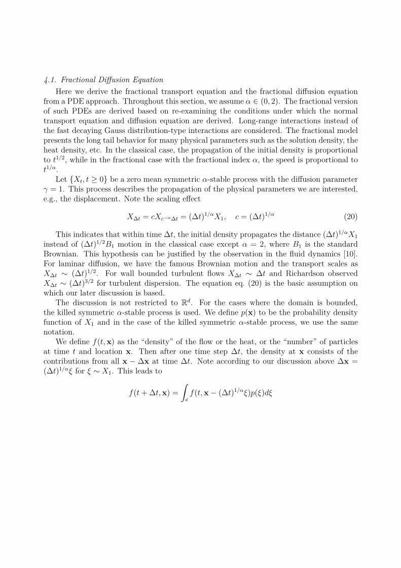
4.1. Fractional Diffusion EquationHere we derive the fractional transport equation and the fractional diffusion equation

from a PDE approach. Throughout this section, we assume α ∈ (0, 2). The fractional versionof such PDEs are derived based on re-examining the conditions under which the normaltransport equation and diffusion equation are derived. Long-range interactions instead ofthe fast decaying Gauss distribution-type interactions are considered. The fractional modelpresents the long tail behavior for many physical parameters such as the solution density, theheat density, etc. In the classical case, the propagation of the initial density is proportionalto t1/2, while in the fractional case with the fractional index α, the speed is proportional tot1/α.

Let Xt, t ≥ 0 be a zero mean symmetric α-stable process with the diffusion parameterγ = 1. This process describes the propagation of the physical parameters we are interested,e.g., the displacement. Note the scaling effect

X∆t = cXc−α∆t = (∆t)1/αX1, c = (∆t)1/α (20)

This indicates that within time ∆t, the initial density propagates the distance (∆t)1/αX1

instead of (∆t)1/2B1 motion in the classical case except α = 2, where B1 is the standardBrownian. This hypothesis can be justified by the observation in the fluid dynamics [10].For laminar diffusion, we have the famous Brownian motion and the transport scales asX∆t ∼ (∆t)1/2. For wall bounded turbulent flows X∆t ∼ ∆t and Richardson observedX∆t ∼ (∆t)3/2 for turbulent dispersion. The equation eq. (20) is the basic assumption onwhich our later discussion is based.

The discussion is not restricted to Rd. For the cases where the domain is bounded,the killed symmetric α-stable process is used. We define p(x) to be the probability densityfunction of X1 and in the case of the killed symmetric α-stable process, we use the samenotation.

We define f(t,x) as the “density” of the flow or the heat, or the “number” of particlesat time t and location x. Then after one time step ∆t, the density at x consists of thecontributions from all x − ∆x at time ∆t. Note according to our discussion above ∆x =(∆t)1/αξ for ξ ∼ X1. This leads to

f(t+∆t,x) =

∫d

f(t,x− (∆t)1/αξ)p(ξ)dξ

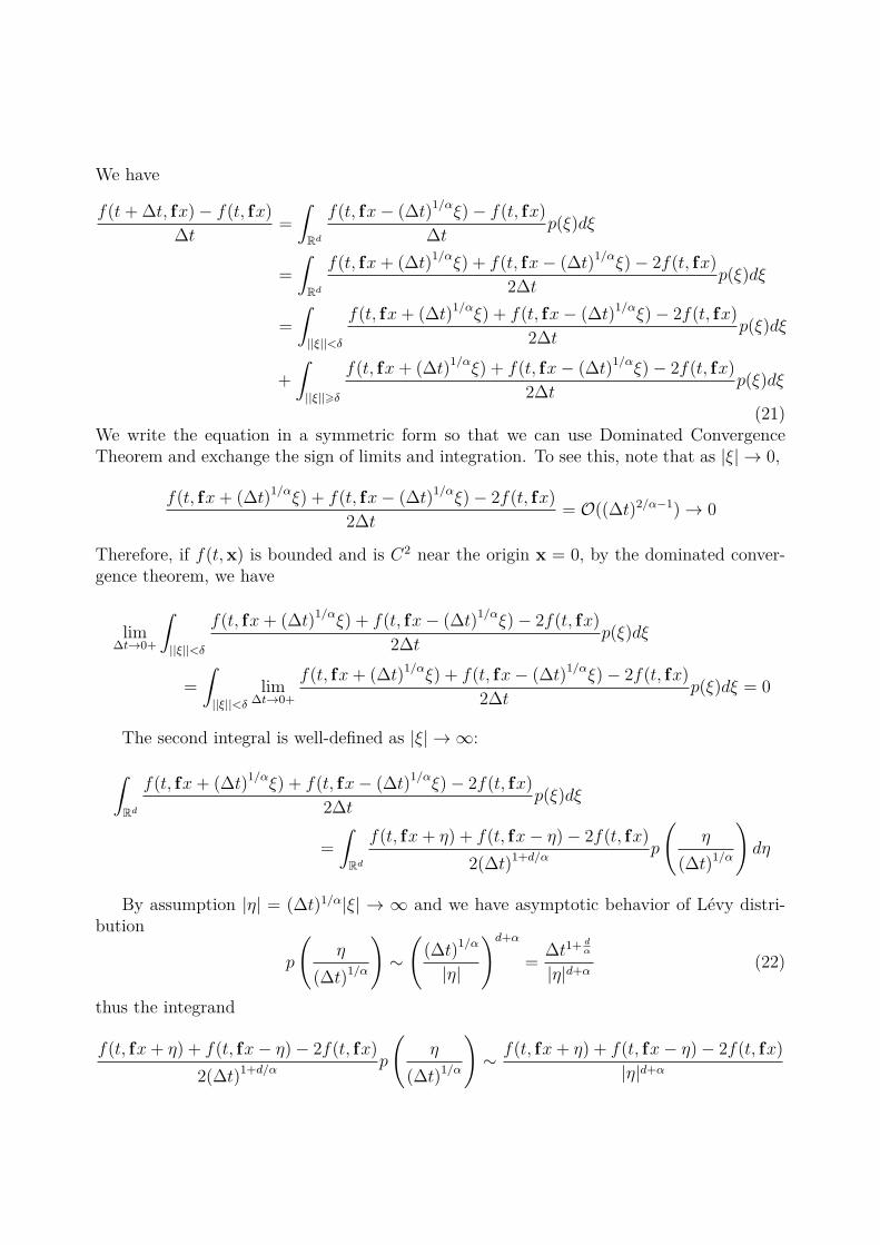
We have

f(t+∆t, fx)− f(t, fx)

∆t=

∫Rd

f(t, fx− (∆t)1/αξ)− f(t, fx)

∆tp(ξ)dξ

=

∫Rd

f(t, fx+ (∆t)1/αξ) + f(t, fx− (∆t)1/αξ)− 2f(t, fx)

2∆tp(ξ)dξ

=

∫||ξ||<δ

f(t, fx+ (∆t)1/αξ) + f(t, fx− (∆t)1/αξ)− 2f(t, fx)

2∆tp(ξ)dξ

+

∫||ξ||⩾δ

f(t, fx+ (∆t)1/αξ) + f(t, fx− (∆t)1/αξ)− 2f(t, fx)

2∆tp(ξ)dξ

(21)We write the equation in a symmetric form so that we can use Dominated ConvergenceTheorem and exchange the sign of limits and integration. To see this, note that as |ξ| → 0,

f(t, fx+ (∆t)1/αξ) + f(t, fx− (∆t)1/αξ)− 2f(t, fx)

2∆t= O((∆t)2/α−1) → 0

Therefore, if f(t,x) is bounded and is C2 near the origin x = 0, by the dominated conver-gence theorem, we have

lim∆t→0+

∫||ξ||<δ

f(t, fx+ (∆t)1/αξ) + f(t, fx− (∆t)1/αξ)− 2f(t, fx)

2∆tp(ξ)dξ

=

∫||ξ||<δ

lim∆t→0+

f(t, fx+ (∆t)1/αξ) + f(t, fx− (∆t)1/αξ)− 2f(t, fx)

2∆tp(ξ)dξ = 0

The second integral is well-defined as |ξ| → ∞:

∫Rd

f(t, fx+ (∆t)1/αξ) + f(t, fx− (∆t)1/αξ)− 2f(t, fx)

2∆tp(ξ)dξ

=

∫Rd

f(t, fx+ η) + f(t, fx− η)− 2f(t, fx)

2(∆t)1+d/αp

(η

(∆t)1/α

)dη

By assumption |η| = (∆t)1/α|ξ| → ∞ and we have asymptotic behavior of Lévy distri-bution

p

(η

(∆t)1/α

)∼

((∆t)1/α

|η|

)d+α

=∆t1+

dα

|η|d+α(22)

thus the integrand

f(t, fx+ η) + f(t, fx− η)− 2f(t, fx)

2(∆t)1+d/αp

(η

(∆t)1/α

)∼ f(t, fx+ η) + f(t, fx− η)− 2f(t, fx)

|η|d+α

the denominator ensures that it is integrable to the infinity. The derivation also indicatesthat

∂f(t,x)

∂t= lim

∆→0+

∫|ξ|≥δ

f(t, fx+ η) + f(t, fx− η)− 2f(t, fx)

2(∆t)1+d/αp

(η

(∆t)1/α

)dx

= Cα,d

∫Rd

f(t, fx+ η) + f(t, fx− η)− 2f(t, fx)

|η|d+αdx (23)

where Cα,d is determined by the asymptotic behavior eq. (22). We immediately identify theright hand side of eq. (23) as the fractional Laplacian up to a constant. And we obtain thefollowing fractional diffusion equation

∂f(t,x)

∂t= −(−∆)α/2f(t,x) (24)

Note that we have assumed the symmetric α-stable process has the dispersion coefficientγ = 1. By varying this coefficient, we are able to obtain different diffusion coefficients. Thecoefficient will have the dimension

(length)α

(time)Remark 1. The above argument only holds for α ∈ (0, 2). The normal diffusion equationis recovered when α = 2. In this case, the second integral in eq. (21) tends to 0 as we pass∆t to 0. The first integral yields the Laplacian ∆u(x).

4.2. Fractional Advection-diffusion EquationLike in the Brownian case, the symmetric α-stable process can also lead to diffusion

with an additional velocity field v and external field. The only difference from the fractionaldiffusion equation is that the stationary state is invariant under the transform x → x +v∆t) (i.e. Galilei invariant). We have

f(x+ v∆t, t+∆t) =

∫Rn

f(x− (∆t)αξ, t)p(ξ)dξ

Note that we have

f(x+ v∆t, t+∆t) = f(x, t) + v · ∇f(x, t)∆t+∂f(x, t)

∂t∆t+O((∆t)2)

Similar to the derivation of fractional diffusion equation, we obtain the fractionaladvection-diffusion equation

∂f(t,x)

∂t+ v · ∇f(t,x) = Cα,d

∫Rd

f(t, fx+ η) + f(t, fx− η)− 2f(t, fx)

|η|d+αdη

which is∂f(t,x)

∂t+ v · ∇f(t,x) = −(−∆)α/2f(t,x) (25)

4.3. Fokker-Planck EquationUnder certain conditions, the diffusion equation can be seen as a special case of the

Fokker-Planck equation. In this section, we derive the fractional Fokker-Planck equation inΩ = Rd.

Consider the LévyXt = x+ Jt, t ≥ 0

By Itô’s formula eq. (12) we have

f(Xt) = f(x) + cα,d

∫ t

0

∫Rd

[f(Xs)− f(Xs−)−Df(Xs−) · (Xs −Xs−)]ν(ds, dx)

We have

Ex[f(Xt)]− f(x) = cα,dE[∫ t

0

∫Rd

[f(Xs)− f(Xs−)−Df(Xs−) · (Xs −Xs−)]ν(ds, dx)

](26)

Consider the transition probabilityPr(Xt ∈ y + dx|X0 = x) = Pt(x,y)dx

and by definition we haveEx[f(Xt)] =

∫x∈Ω

Pt(x,y)dx

Combining with eq. (26) we have∫Ω

f(y)Pt(x,y)dy − f(x) = cα,dEx

[∫ t

0

∫Rd

[f(Xs)− f(Xs−)−Df(Xs−) · (Xs −Xs−)]ν(ds, dx)

]= −Ex

[∫ t

0

(−∆)α/2f(Xs−)ds

]= −

∫ t

0

(∫Ω

[(−∆)α/2f(y)]Ps(x,y)dy

)ds

= −∫Ω

f(y)

(∫ t

0

(−∆)α/2y Ps(x,y)ds

)dy (27)

where in eq. (27) we have performed integration by parts and (−∆)α/2y is the fractional

Laplacian with respect to the y variable.Divide both sides by t and let t → 0, we have

∂Pt(x,y)

∂t= −(−∆)α/2y Pt(x,y) (28)

The initial condition for eq. (28) is given byPt(x,y) → δ(x,y), t → 0

In this case, we have natural boundary conditions, which is the decay to zero and nor-malization

Pt(x,y) = 0,y → ∞;

∫Ω

Pt(x,y)dy = 1

5. Fractional PDE in the Bounded Domain

5.1. The Fractional Poisson ProblemIt is not difficult to realize that the deriving of the linear partial differential equations

in the bounded domain, except that we need to take care of the boundary conditions.Before we discuss the derivation of the linear PDEs with the fractional Laplacian, we first

consider the homogeneous fractional Poisson problem, which can be seen as the stationaryequation of the diffusion equation

(−∆)α/2∗ u(x) = f(x) x ∈ Ω (29)u(x) = 0 x ∈ Ωc or ∂Ω

where the boundary conditions depend on the operator (−∆)α/2∗ we use.

The treatment of the boundary conditions for the initial-boundary value problemeqs. (24), (25) and (28) is essentially as the treatment of eq. (29) and therefore we will onlydiscuss how to impose boundary conditions on eq. (29).

The Integral Fractional LaplacianThe most direct way is to extend the derivation of the fractional PDEs in the bounded

domain is to extend the solution u(t, ·) to Rd. In this case, particles (or probabilities, etc.)at location x and time t +∆t may come from some locations x− (∆t)1/αξ outside Ω. Thescalar u(t, ·) outside Ω is always fixed to 0. It leads to the integral fractional Laplacian.

When the integral fractional Laplacian definition is used, the underlying stochastic pro-cess is a killed symmetric α-stable process. It is possible that Xt ends up at any point x ∈ Ωc

and therefore the well-posed Dirichlet problem is given by

(−∆)α/2I u(x) = f x ∈ Ω

u(x) = 0 x ∈ Ωc

The Spectral Fractional LaplacianDue to the spectral structure of the solution

u(x) =∞∑i=1

uiφi(x)

it is sufficient to specify the boundary values, i.e., the well-posed problem is

(−∆)α/2S u(x) = f x ∈ Ω

u(x) = 0 x ∈ ∂Ω

This can also be understood from its underlying stochastic process: we first kill the Brownianmotion Xt at the first exit time of Xt from the domain Ω and then we subordinate the killedBrownian motion using the α/2-stable subordinator. Only the boundary value is involvedin eq. (18).

The Regional Fractional LaplacianThe boundary condition for this case is more complicated than the other two. The

censored stable process can be obtained by piecing together of killed stable process [30]. Itis shown in [30] that if 0 < α ≤ 1, then the censored α-stable process in Ω is essentially thereflected α-stable process (Xt)t≥0 and if 1 < α < 2, the censored α-stable process in Ω isidentified as a proper subprocess of (Xt)t≥0 killed upon leaving Ω.

It is proved in [31] that (Xt)t≥0 can be refined to be a Feller process starting from eachpoint of Ω, which admits a Hölder continuous transition density function. It is known thatif α < 1 the censored α-stable process will never approach ∂Ω while for α ≥ 1, Xt has finitelife time and take values on ∂Ω. This behavior has remarkable impact on the well-posednessof the Dirichlet problem eq. (29): if 1 < α < 2, the problem

(−∆)α/2R u(x) = f x ∈ Ω

u(x) = 0 x ∈ ∂Ω

is well-posed.In the case 0 < α ≤ 1, we have [32]

Hα/2(Ω) = Hα/20 (Ω) (30)

where Hα/2 is the fractional Sobolev space. Here eq. (30) implies the boundary conditionmakes no sense since the solution always below to H

α/20 (Ω).

5.2. Fractional PDEs in the Bounded DomainWith the boundary condition in the last section, eqs. (24) and (25) can be immediately

extended to the bounded domain Ω. For the Fokker-Planck equation, a key ingredient foreq. (28) to hold on a bounded domain is the integration by parts formula eq. (19). Thederivation eq. (27) can be carried out without change for the bounded Ω (using eq. (18))

5.3. Remarks on 1D CaseIn this section, we consider the integral fractional Laplacian.It is known that on the domain Rd, many definitions for the fractional Laplacian, such as

the integral formulation, the spectral formulation, the Neumann-Dirichlet map formulation,etc., are all equivalent [12]. In one dimension, we can actually make an explicit connectionbetween the fractional Laplacian and the fractional derivatives [33]

(−∆)α/2u(x) =−∞Dα

xu(x) + xDα∞u(x)

2 cos(απ/2)(31)

where −∞Dαx and xD∞ are the Riemann-Liouville derivative

aDαxu(x) =

1

Γ(m− α)

dm

dtm

∫ x

a

(x− τ)m−α−1u(τ)dτ

xDαb u(x) =

1

Γ(m− α)

dm

dtm

∫ b

x

(τ − x)m−α−1u(τ)dτ

where m− 1 ≤ α < m ∈ Z+ [34].In the case we use a bounded domain (a, b), and assume u(τ) = 0,∀τ ∈ [a, b]c,

−∞Dαau(x) =

1

Γ(m− α)

dm

dtm

∫ a

−∞(x− τ)m−α−1u(τ)dτ = 0

and likewise bDα∞u(x) = 0, thus the definition eq. (31) becomes a “local” one

(−∆)α/2u(x) =aD

αxu(x) + xD

αb u(x)

2 cos(απ/2),∀x ∈ [a, b] (32)

But eq. (32) should be understand as (31) plus the zero Dirichlet boundary condition. Thatis to say, it is not correct to impose nonzero “boundary” condition on eq. (32), which indeedis ill-posed when we require u(a) and/or u(b) to be a fixed nonzero value.

6. Conclusion

We studied the fractional Laplacian in Rd and the bounded domain, with an emphasize onthe probabilistic interpretation. For the bounded domain, there are different definitions forthe fractional Laplacian, and we discuss three of those, i.e., the integral fractional Laplacian,the spectral fractional Laplacian, and the regional fractional Laplacian. These operators aregenerators of different stochastic process. Starting from the probabilistic interpretation, wederived the fractional diffusion, the advection-diffusion and the Fokker-Planck equations.Justification for the Dirichlet-type boundary conditions are provided using the underlyingstochastic process.

The integral fractional Laplacian has the distinct feature that the point values dependson the function values in Rd. The other two operators only depend on the values in Ω.However, they are all nonlocal operators in that value a point involves the values of thefunction far away from that point.

We believe this note can serve to clarify many confusions about the fractional PDEs in-volving the fractional Laplacian and also emphasize on the interpretability of the underlyingstochastic process for the PDEs.

7. References[1] Wen Chen. Soft matter and fractional mathematics: insights into mesoscopic quantum and time-space

structures. arXiv preprint cond-mat/0405345, 2004.[2] Serena Dipierro, Giampiero Palatucci, and Enrico Valdinoci. Dislocation dynamics in crystals: a macro-

scopic theory in a fractional laplace setting. Communications in Mathematical Physics, 333(2):1061–1105, 2015.

[3] Oleg G Bakunin. Turbulence and diffusion: scaling versus equations. Springer Science & BusinessMedia, 2008.

[4] Mauro Bologna, Constantino Tsallis, and Paolo Grigolini. Anomalous diffusion associated with nonlin-ear fractional derivative fokker-planck-like equation: Exact time-dependent solutions. Physical ReviewE, 62(2):2213, 2000.

[5] Wojbor A Woyczyński. Lévy processes in the physical sciences. In Lévy processes, pages 241–266.Springer, 2001.

[6] Paolo Gatto and Jan S Hesthaven. Numerical approximation of the fractional Laplacian via hp-finiteelements, with an application to image denoising. Journal of Scientific Computing, 65(1):249–270,2015.

[7] Juan Luis Vázquez. Nonlinear diffusion with fractional Laplacian operators. In Nonlinear partialdifferential equations, pages 271–298. Springer, 2012.

[8] W. Chen and S. Holm. Fractional Laplacian time-space models for linear and nonlinear lossy mediaexhibiting arbitrary frequency power-law dependency. The Journal of the Acoustical Society of America,115(4):1424–1430, 2004.

[9] Rama Cont and Ekaterina Voltchkova. A finite difference scheme for option pricing in jump diffusionand exponential lévy models. SIAM Journal on Numerical Analysis, 43(4):1596–1626, 2005.

[10] Brenden P Epps and Benoit Cushman-Roisin. Turbulence modeling via the fractional Laplacian. arXivpreprint arXiv:1803.05286, 2018.

[11] Xavier Ros et al. Integro-differential equations: Regularity theory and pohozaev identities. 2014.[12] Mateusz Kwaśnicki. Ten equivalent definitions of the fractional laplace operator. Fractional Calculus

and Applied Analysis, 20(1):7–51, 2017.[13] René L. Schilling. An introduction to Lévy and feller processes. advanced courses in mathematics -

crm barcelona 2014. 03 2016.[14] Levy.pdf. http://www.math.utah.edu/~davar/ps-pdf-files/Levy.pdf. (Accessed on 05/03/2018).[15] n-d_spherical_coordinates.pdf. http://www.ams.sunysb.edu/~wshih/mathnotes/n-D_Spherical_coordinates.pdf.

(Accessed on 04/30/2018).[16] Dlmf: 5.12 beta function. https://dlmf.nist.gov/5.12. (Accessed on 04/30/2018).[17] Richard F. Bass. Stochastic differential equations with jumps.[18] Zongfei Fu and Zenghu Li. Stochastic equations of non-negative processes with jumps. Stochastic

Processes and their Applications, 120(3):306 – 330, 2010.[19] Aleksander Weron and Rafal Weron. Computer simulation of lévy α-stable variables and processes. In

Chaos-The Interplay Between Stochastic and Deterministic Behaviour, pages 379–392. Springer, 1995.[20] Yu Davydov and AV Nagaev. On two aproaches to approximation of multidimensional stable laws.

Journal of multivariate analysis, 82(1):210–239, 2002.[21] Luis Caffarelli and Luis Silvestre. An extension problem related to the fractional Laplacian. Commu-

nications in partial differential equations, 32(8):1245–1260, 2007.[22] Andrea Bonito and Joseph Pasciak. Numerical approximation of fractional powers of elliptic operators.

Mathematics of Computation, 84(295):2083–2110, 2015.[23] Giovanni Molica Bisci, Vicentiu D Radulescu, and Raffaella Servadei. Variational methods for nonlocal

fractional problems, volume 162. Cambridge University Press, 2016.[24] Andreas E Kyprianou, Ana Osojnik, and Tony Shardlow. Unbiased ‘walk-on-spheres’ monte carlo

methods for the fractional Laplacian. IMA Journal of Numerical Analysis, 2016.[25] Panki Kim, Renming Song, and Zoran Vondraček. Potential theory of subordinate killed Brownian

motion. arXiv preprint arXiv:1610.00872, 2016.[26] Renming Song and Zoran Vondraček. Potential theory of subordinate killed Brownian motion in a

domain. Probability theory and related fields, 125(4):578–592, 2003.[27] Krzysztof Bogdan, Krzysztof Burdzy, and Zhen-Qing Chen. Censored stable processes. Probability

theory and related fields, 127(1):89–152, 2003.[28] Qing-Yang Guan and Zhi-Ming Ma. Reflected symmetric α-stable processes and regional fractional

Laplacian. Probability theory and related fields, 134(4):649–694, 2006.[29] Qing-Yang Guan. Integration by parts formula for regional fractional Laplacian. Communications in

mathematical physics, 266(2):289–329, 2006.[30] Krzysztof Bogdan, Krzysztof Burdzy, and Zhen Qing Chen. Censored stable processes. Probability

Theory and Related Fields, 127(1):89–152, 2003.[31] Zhen-Qing Chen and Takashi Kumagai. Heat kernel estimates for stable-like processes on d-sets.

Stochastic Processes and their applications, 108(1):27–62, 2003.[32] What are the classical boundary conditions for the fractional laplace operator?

http://www.public.iastate.edu/~stinga/Warma.pdf. (Accessed on 05/04/2018).[33] Yanghong Huang and Adam Oberman. Finite difference methods for fractional Laplacians. arXiv

preprint arXiv:1611.00164, 2016.[34] Changpin Li, Deliang Qian, and YangQuan Chen. On Riemann-Liouville and Caputo derivatives.

Discrete Dynamics in Nature and Society, 2011, 2011.