Comment on the Campbell-Cochrane

Habit Model

Lars Ljungqvist Harald Uhlig∗

August 5, 2010

Abstract

Campbell and Cochrane (1999) formulate a model that successfully explains a wide

variety of asset pricing puzzles, by augmenting the standard power utility function

with a time-varying “external habit”, that adapts nonlinearly to current and past av-

erage consumption in the economy. We demonstrate that their preference specification

has the unusual implications that habit can move negatively with consumption, and

that the social marginal utility can be negative. As a result, government interven-

tions that occasionally destroy part of the endowment can lead to substantial welfare

improvements.

JEL code: E21, E44, G12

∗Ljungqvist: Stockholm School of Economics and New York University (email: lars.ljungqvist@hhs.se);Uhlig: University of Chicago (email: huhlig@uchicago.edu). We thank Fernando Alvarez and John Cochranefor criticisms and suggestions on our earlier exploration of the properties of the Campbell-Cochrane prefer-ence specification. The present exposition has benefitted much from the comments of the editor and threeanonymous referees. Ljungqvist’s research was supported by a grant from the Jan Wallander and TomHedelius Foundation. Uhlig’s research has been supported by the NSF grant SES-0922550.

1 Introduction

Campbell and Cochrane (1999, hereafter denoted C-C) formulate a model that successfully

explains a wide variety of asset pricing puzzles, including a high equity premium, procyclical

variation of stock prices, countercyclical variation of stock market volatility, and a low and

smooth riskfree rate. These remarkable results are achieved by augmenting the standard

power utility function with a time-varying subsistence level, or “external habit”, that adapts

nonlinearly to current and past average consumption in the economy. Given the break-

through in matching key asset pricing facts as well as the successful adoption of the C-C

preferences in a number of other applications, it is all the more important to fully understand

the implications of these modeling choices.

We show that the assertions by Campbell and Cochrane (1999, p. 212, p. 246) that

“habit moves nonnegatively with consumption everywhere,” and that “more consumption

is always socially desirable” are incorrect. As a result, government interventions that occa-

sionally destroy part of the endowment can lead to substantial welfare improvements. Large

interventions are not required: welfare improves already with the rather tiny one-time de-

struction of less than one tenth of a percent of aggregate consumption. Hence, Campbell

and Cochrane’s (1999, pp. 245–247) attempt to map their results into a version of the model

with internal habit formation must be reconsidered. Households faced with such an internal

habit would themselves choose to periodically destroy endowments.

Our results are true for the specific formulation of Campbell and Cochrane, and due

to their particular and nonlinear specification of the evolution for the habit. They are

not true for habit specifications in general. Indeed, for a more conventional linear habit

formulation, one can show that welfare must decrease along the balanced growth path, if

parts of consumption are destroyed: the utility gain later is outweighed by the initial utility

loss.

2 The model

The utility function of the representative agent is

E0

∞∑

t=0

δt (Ct −Xt)1−γ − 1

1 − γ, (1)

1

where δ is the subjective time discount factor and Xt is the level of external habit. A

conventional linear external habit formulation specifies that

Xt+1 = µXt + αCat , (2)

where Ca denotes average consumption by all agents in the economy, and µ and α are

parameters.

Campbell and Cochrane (1999) proceed differently. They postulate a process for the

economy’s surplus consumption ratio, Sat ≡ (Ca

t −Xt)/Cat . Using lowercase letters to indicate

logarithms, they assume that the logarithm of the surplus consumption ratio evolves as a

heteroscedastic AR(1) process,

sat+1 = (1 − φ)s+ φsa

t + λ(sat )

(

cat+1 − cat − g)

, (3)

where φ ∈ [0, 1), g and s are parameters, and the function λ(sa) is given by

λ(sa) =

S−1√

1 − 2(sa − s) − 1, sa ≤ smax;

0, sa ≥ smax;(4)

with smax = s +(

1 − S2)

/2. The parameter s is the logarithm of the steady-state surplus

consumption ratio S, and Campbell and Cochrane set g equal to the logarithm of the mean

consumption gross growth rate G. It can be shown that the C-C formulation and the

conventional linear habit formulation in equation (2) share the same steady state if µ = Gφ

and α = G(1 − φ)(1 − S).

Campbell and Cochrane consider a pure endowment economy. Let Yt be the per capita

endowment in period t. Endowment growth is modeled as an i.i.d. lognormal process,

∆yt+1 = g + νt+1, νt+1 ∼ i.i.d. N (0, σ2). (5)

The equilibrium outcome in a laissez-faire market economy is that consumption equals en-

dowment, cat = yt, since the private marginal utility under the C-C preference specification is

strictly positive. But, contrary to Campbell and Cochrane’s assertion, we shall demonstrate

that the social marginal utility can be negative. Specifically, we investigate the welfare effects

when a social planner destroys some of the endowment.

Let ψt denote the logarithm of the fraction of the endowment that the representative

agent gets to consume in period t, i.e., ψt ≡ cat − yt ≤ 0. The welfare of the representative

2

agent can then be written as

E0

∞∑

t=0

δt (Sat C

at )1−γ − 1

1 − γ= E0

∞∑

t=0

δt exp ((1 − γ)(sat + ψt + yt)) − 1

1 − γ, (6)

and the law of motion for the log surplus consumption ratio can be expressed as

sat+1 = (1 − φ)s+ φsa

t + λ(sat ) (ψt+1 − ψt + νt+1) , (7)

where we have used equation (5) to substitute out for g. From now on, we will leave out the

superscript a since outcomes for the representative agent and economy-wide averages are the

same in an equilibrium.

3 Social marginal utility can be negative

If Campbell and Cochrane had been correct when asserting that the social marginal utility is

always positive in their model, the highest welfare would be attained by setting ψt = 0 in all

periods. However, Campbell and Cochrane only prove that an infinitesimal destruction of the

endowment leads to a welfare loss. To illustrate our surprising finding that noninfinitesimal

destructions can increase welfare under the C-C habit formulation, it is instructive to consider

a one-time perturbation from a steady state.

Consider an economy in a non-stochastic steady state with endowment and consumption

growing at a constant growth rate G ≥ 1. The parameter restriction that ensures a bounded

objective function is

δG1−γ < 1 . (8)

Suppose now that the social planner destroys part of the endowment in one single period,

denoted period 0. Thus, we have log(C0/Y0) = ψ < 0, and the sequences of the logarithms

of consumption and the surplus consumption ratio evolve as follows

c0(ψ) = y0 + ψ < y0 , (9a)

ct(ψ) = yt , for all t ≥ 1; (9b)

s0(ψ) = s+ λψ < s , (9c)

st(ψ) = s− φt−1ψ[

λ(s+ λψ) − φλ]

> s , for all t ≥ 1; (9d)

3

where λ ≡ λ(s). Evidently, the representative agent’s utility falls in period 0 because both

his consumption level and the surplus consumption ratio decline relative to the steady state.

But the utilities in all future periods increase due to a higher surplus consumption ratio that

asymptotically returns to its steady-state value. The question is whether the discounted sum

of these changes in utilities produce a welfare gain or a welfare loss.

After eliminating the constant terms involving −1/(1− γ) in the preference specification

and dividing through by exp ((1 − γ)y0), the discounted life-time utility of the described

perturbation can be expressed as

W (ψ) ≡exp ((1 − γ)(s0(ψ) + ψ))

1 − γ+

∞∑

t=1

δt exp ((1 − γ)(st(ψ) + tg))

1 − γ(10)

with the derivative

W ′(ψ) = (1 + λ) exp ((1 − γ)(s0(ψ) + ψ)) +

∞∑

t=1

δt[

φt−1s′1(ψ)]

exp ((1 − γ)(st(ψ) + tg)) , (11)

where

s′1(ψ) = −[

λ(s+ ψλ) − φλ]

− ψλ λ′(s+ ψλ) < 0. (12)

The derivative s′1 is negative since ψ < 0 and λ is a decreasing function. Thus, whether

welfare marginally increases or decreases at negative values of ψ depends on whether the

first or the second term in equation (11) dominates numerically. It can be shown that

welfare is globally increasing with a conventional linear habit formulation: there, endowment

destruction in a steady state always leads to a welfare loss. This is also true locally along the

steady-state path for the C-C preferences.1 This should come as no surprise since Campbell

and Cochrane (1999, p. 246) prove that the social marginal utility is positive in their model.

More specifically, they show that the social marginal utility is positive for infinitesimal

perturbations when the endowment follows a random walk. When setting growth equal to

1We verify that an infinitesimal endowment destruction decreases welfare under the C-C preferences;

W ′(0) = (1 + λ)S1−γ −∞∑

t=1

δtφt−1(1 − φ)λ[

SGt]1−γ

=1 − φδG1−γ + (1 − δG1−γ)λ

1 − φδG1−γS1−γ > 0 ,

where the convergence of the infinite sum and the strict inequality follow from φ ∈ [0, 1) and parameterrestriction (8). Thus, in the neighborhood around the steady-state growth path, welfare is strictly increasingin the fraction of the endowment that is consumed.

4

zero in our calculations, we have a constant endowment level or a degenerate random walk.

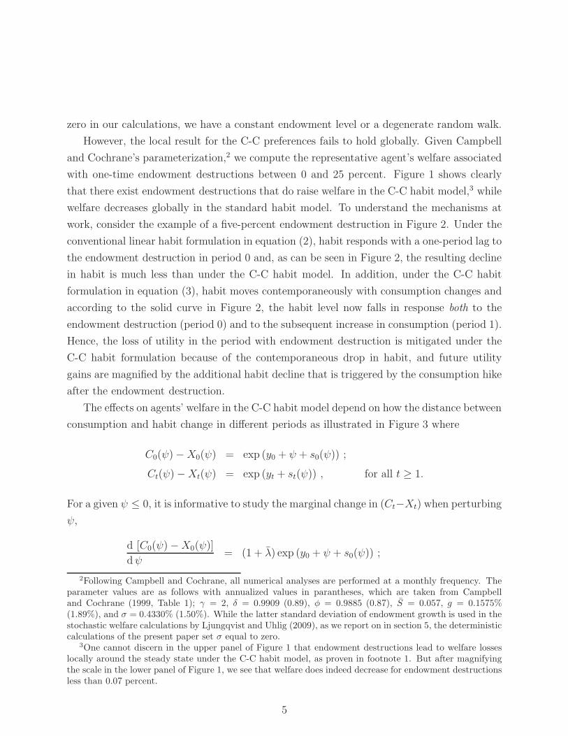
However, the local result for the C-C preferences fails to hold globally. Given Campbell

and Cochrane’s parameterization,2 we compute the representative agent’s welfare associated

with one-time endowment destructions between 0 and 25 percent. Figure 1 shows clearly

that there exist endowment destructions that do raise welfare in the C-C habit model,3 while

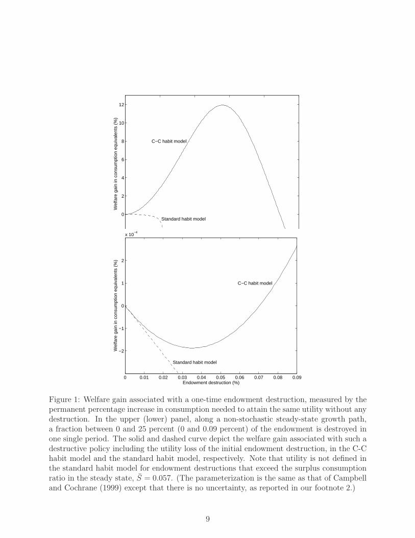
welfare decreases globally in the standard habit model. To understand the mechanisms at

work, consider the example of a five-percent endowment destruction in Figure 2. Under the

conventional linear habit formulation in equation (2), habit responds with a one-period lag to

the endowment destruction in period 0 and, as can be seen in Figure 2, the resulting decline

in habit is much less than under the C-C habit model. In addition, under the C-C habit

formulation in equation (3), habit moves contemporaneously with consumption changes and

according to the solid curve in Figure 2, the habit level now falls in response both to the

endowment destruction (period 0) and to the subsequent increase in consumption (period 1).

Hence, the loss of utility in the period with endowment destruction is mitigated under the

C-C habit formulation because of the contemporaneous drop in habit, and future utility

gains are magnified by the additional habit decline that is triggered by the consumption hike

after the endowment destruction.

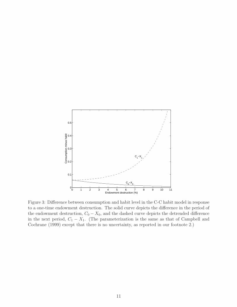
The effects on agents’ welfare in the C-C habit model depend on how the distance between

consumption and habit change in different periods as illustrated in Figure 3 where

C0(ψ) −X0(ψ) = exp (y0 + ψ + s0(ψ)) ;

Ct(ψ) −Xt(ψ) = exp (yt + st(ψ)) , for all t ≥ 1.

For a given ψ ≤ 0, it is informative to study the marginal change in (Ct−Xt) when perturbing

ψ,

d [C0(ψ) −X0(ψ)]

dψ= (1 + λ) exp (y0 + ψ + s0(ψ)) ;

2Following Campbell and Cochrane, all numerical analyses are performed at a monthly frequency. Theparameter values are as follows with annualized values in parantheses, which are taken from Campbelland Cochrane (1999, Table 1); γ = 2, δ = 0.9909 (0.89), φ = 0.9885 (0.87), S = 0.057, g = 0.1575%(1.89%), and σ = 0.4330% (1.50%). While the latter standard deviation of endowment growth is used in thestochastic welfare calculations by Ljungqvist and Uhlig (2009), as we report on in section 5, the deterministiccalculations of the present paper set σ equal to zero.

3One cannot discern in the upper panel of Figure 1 that endowment destructions lead to welfare losseslocally around the steady state under the C-C habit model, as proven in footnote 1. But after magnifyingthe scale in the lower panel of Figure 1, we see that welfare does indeed decrease for endowment destructionsless than 0.07 percent.

5

d [Ct(ψ) −Xt(ψ)]

dψ= φt−1s′1(ψ) exp (yt + st(ψ)) , for all t ≥ 1.

We can see that the derivative in period 0 gets muted at low values of ψ, i.e., at higher levels of

endowment destruction, while the opposite is true for the corresponding derivatives in future

periods. In fact, the multiplicative term s′1 as given in equation (12) becomes arbitrarily

large and negative when ψ is driven to ever lower values and therefore, the associated loss

in (Ct − Xt) for t ≥ 1, becomes arbitrarily large when reducing the amount of endowment

destruction in period 0. This in turn implies that (Ct−Xt) for t ≥ 1, must take on arbitrarily

large values when computed at ever lower values of ψ. Figure 3 depicts the exploding outcome

for (C1−X1) when increasing the amount of endowment destruction in period 0. Behind the

exploding outcome for (C1 − X1) in Figure 3 lies a critical property of the C-C preference

specifiation: habit can move negatively with consumption.

4 Habit can move negatively with consumption

In Figure 2, the consumption hike in period 1 does not increase but rather decreases the

habit level in the C-C habit model. Hence, Campbell and Cochrane’s claim that habit moves

nonnegatively with consumption everywhere is incorrect. In fact, habit can fall contempora-

neously with a rise in consumption even locally around the steady state. After differentiating

the law of motion for the surplus consumption ratio in equation (3), we obtain

dxt+1

dct+1

= 1 −λ(st)

exp(−st+1) − 1.

In the steady state, st = st+1 = s, so the parameterization of the function λ(s) in equation

(4) guarantees that dx/dc = 0 at the steady state. Next, we calculate the second derivative,

d2xt+1

dc2t+1

= −λ(st)

2

[exp(−st+1) − 1]2exp(−st+1) ≤ 0,

and the expression is strictly negative at the steady state. This establishes that there is a

region around the steady state in which habit moves negatively with consumption.4

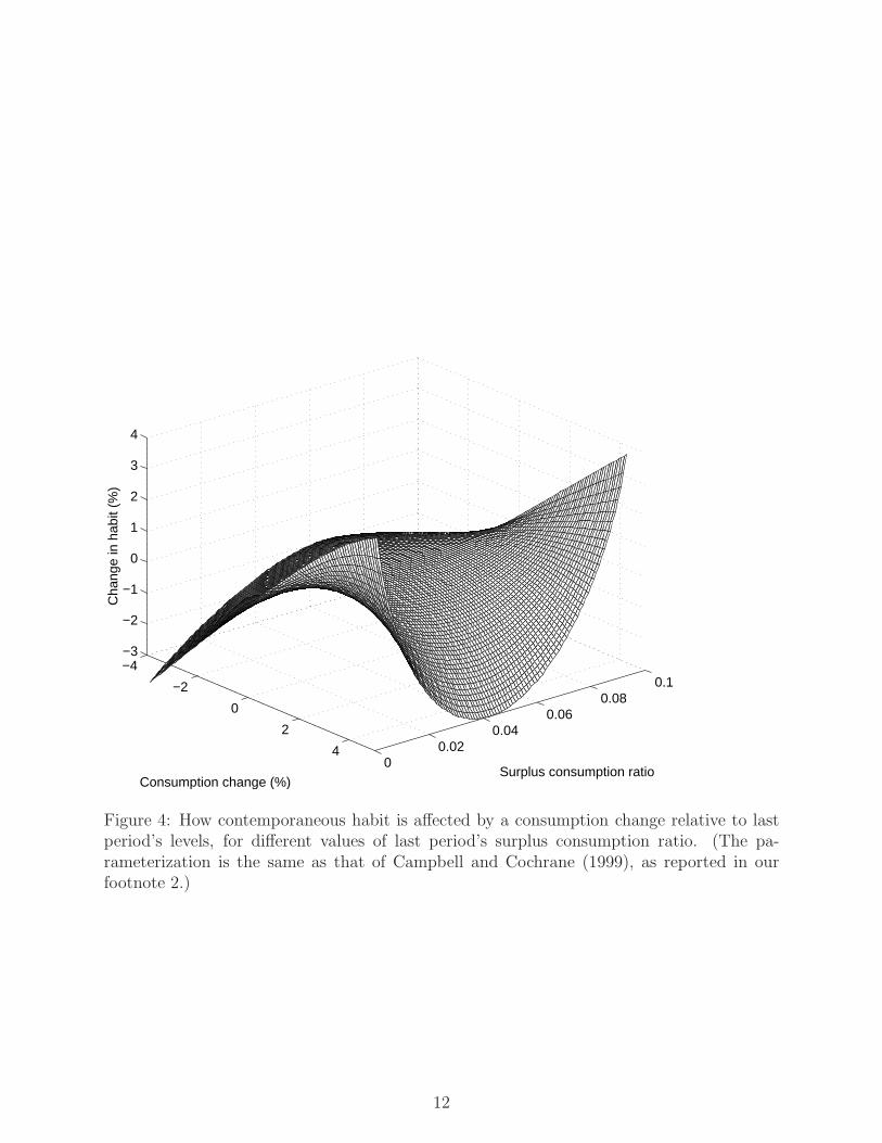
Based on Campbell and Cochrane’s parameterization (see our footnote 2), Figure 4 maps

out the relationship between consumption changes and movements in the habit level. In

particular, for a given value of last period’s surplus consumption ratio, the figure depicts

4We are thankful to John Cochrane for suggesting this exposition of our argument.

6

how contemporaneous habit responds to percentage changes in consumption relative to last

period’s levels. As a reference point, the steady-state surplus consumption ratio is 0.057.

It can be seen that the habit level moves negatively with consumption for a wide range of

consumption increases. This property is central to the numerical findings in Ljungqvist and

Uhlig’s (2009) simulations of the C-C framework, which reveal substantial welfare gains of

big as well as small periodic endowment destructions.

5 Concluding remarks

Ljungqvist and Uhlig (2009) calculate that a society of agents with the preferences and

stochastic endowment process of Campbell and Cochrane (1999) would experience a welfare

gain equivalent to a permanent increase of nearly 16% in consumption, if the government

enforced one month of fasting per year, reducing consumption by 10 percent then. The large

welfare improvements associated with the cyclical destruction of endowments can be under-

stood as “investments” in a lower habit level. That is, a period of endowment destruction is

most likely to be followed by a rebounce in consumption next period and this consumption

growth will often be associated with the strange effect of lowering the habit level.

If the Campbell-Cochrane preferences were embedded in an economy with storage or pro-

duction, it would rationalize outcomes of consumption bunching either chosen by households

themselves under internal habit formation or through destabilizing policies by a benevolent

government under external habit formation.5 In calculations not reported here, using the

stochastic endowment process of Campbell and Cochrane, we find large welfare gains from

storing roughly 10 percent of the endowment and consuming the savings in a consumption

binge every other month. To make the households in a laissez-faire economy that consumes

the endowment indifferent to such a policy, consumption would have to be raised by more

than 30 percentage points for the indefinite future.

5By contrast, Ljungqvist and Uhlig (2000) report on how welfare can be improved through policiesof consumption stabilization under catching-up-with-the-Joneses preferences, i.e., the conventional linearexternal habit formulation. In a productivity-shock driven economy, it is shown that such a consumptionexternality calls for an optimal tax policy that affects the economy countercyclically via procyclical taxes,i.e., “cooling” down the economy with higher taxes in booms and lowering taxes in recessions to stimulatethe economy.

7

References

Campbell, John Y. and John H. Cochrane. 1999. By Force of Habit: A Consumption-

Based Explanation of Aggregate Stock Market Behavior. Journal of Political Economy

107 (2):205–251.

Ljungqvist, Lars and Harald Uhlig. 2000. Tax Policy and Aggregate Demand Management

under Catching Up with the Joneses. American Economic Review 90 (3):356–366.

———. 2009. Optimal Endowment Destruction under Campbell-Cochrane Habit Formation.

Working Paper no. 14772. Cambridge, Mass.: National Bureau of Economic Research.

8

0 5 10 15 20 25−2

0

2

4

6

8

10

12

Endowment destruction (%)

Wel

fare

gai

n in

con

sum

ptio

n eq

uiva

lent

s (%

)

Standard habit model

C−C habit model

0 0.01 0.02 0.03 0.04 0.05 0.06 0.07 0.08 0.09

−2

−1

0

1

2

x 10−4

Endowment destruction (%)

Wel

fare

gai

n in

con

sum

ptio

n eq

uiva

lent

s (%

)

Standard habit model

C−C habit model

Figure 1: Welfare gain associated with a one-time endowment destruction, measured by thepermanent percentage increase in consumption needed to attain the same utility without anydestruction. In the upper (lower) panel, along a non-stochastic steady-state growth path,a fraction between 0 and 25 percent (0 and 0.09 percent) of the endowment is destroyed inone single period. The solid and dashed curve depict the welfare gain associated with such adestructive policy including the utility loss of the initial endowment destruction, in the C-Chabit model and the standard habit model, respectively. Note that utility is not defined inthe standard habit model for endowment destructions that exceed the surplus consumptionratio in the steady state, S = 0.057. (The parameterization is the same as that of Campbelland Cochrane (1999) except that there is no uncertainty, as reported in our footnote 2.)

9

−1 0 1 2 3 4 5 6 7 8 9 10

0.9

0.92

0.94

0.96

0.98

1

Time in years

Det

rend

ed h

abit

leve

l and

con

sum

ptio

nConsumption

Standard habit model

C−C habit model

0

1

0

1

−1 0 1 2 3 4 5 6 7 8 9 100

0.01

0.02

0.03

0.04

0.05

0.06

0.07

0.08

0.09

0.1

Time in years

Con

sum

ptio

n m

inus

hab

it

Standard habit model

C−C habit model

Figure 2: Detrended consumption and habit level associated with a five-percent endowmentdestruction in period 0. In the upper panel, the dash-dotted curve depicts the consumptiontime series that bounces back in period 1, and the solid and dashed curve show the habittime series for the C-C habit model and the standard habit model, respectively. In thelower panel, the solid and dashed line depict the difference between the consumption andhabit time series for the C-C habit model and the standard habit model, respectively. (Theparameterization is the same as that of Campbell and Cochrane (1999) except that there isno uncertainty, as reported in our footnote 2.)

10

0 1 2 3 4 5 6 7 8 9 10 110

0.1

0.2

0.3

0.4

0.5

Endowment destruction (%)

Con

sum

ptio

n m

inus

hab

it

C1−X

1

C0−X

0

Figure 3: Difference between consumption and habit level in the C-C habit model in responseto a one-time endowment destruction. The solid curve depicts the difference in the period ofthe endowment destruction, C0 −X0, and the dashed curve depicts the detrended differencein the next period, C1 − X1. (The parameterization is the same as that of Campbell andCochrane (1999) except that there is no uncertainty, as reported in our footnote 2.)

11

−4

−2

0

2

40

0.020.04

0.060.08

0.1

−3

−2

−1

0

1

2

3

4

Surplus consumption ratioConsumption change (%)

Cha

nge

in h

abit

(%)

Figure 4: How contemporaneous habit is affected by a consumption change relative to lastperiod’s levels, for different values of last period’s surplus consumption ratio. (The pa-rameterization is the same as that of Campbell and Cochrane (1999), as reported in ourfootnote 2.)

12

Technical Appendix - not for publication

Appendix

We show that welfare cannot increase by destroying part of the endowment along a steady-

state growth path, given that the external habit level is governed by a conventional linear

law of motion;

Xt = µXt−1 + αCat−1 = αCa

0

t−1∑

j=0

µjGt−1−j + µtX0 ,

where the second equality would hold along the constant growth path. In a steady state,

habit is ensured to be less than consumption if the parameters satisfy

G > µ+ α, (13)

and habit would then grow at the rateG and result in a steady-state ratioXt/Ct = α/(G−µ).

Let Ct, Xt denote the sequence of consumption and habit levels in the steady state,

and consider a one-time perturbation where a fraction 4 ∈ [0, 1 − α/(G − µ)) ≡ Γ of the

endowment is destroyed in period 0: C0 = (1 −4)C0, Ct = Ct for all t ≥ 1; X0 = X0, Xt =

Xt − µt−1α4C0 for all t ≥ 1. Let Ω(4) denote the welfare associated with a perturbation

4, i.e., the preferences in (1) are evaluated at the allocation Ct, Xt. Since Ω′′(4) < 0 for

all 4 ∈ Γ, it suffices to show that Ω′(0) < 0 in order to establish that Ω′(4) < 0 for all

4 ∈ Γ. We can compute

Ω′(0) = −(C0 −X0)−γC0 +

∞∑

t=1

δt(Ct −Xt)−γµt−1αC0 .

After substituting in for the steady-state allocation, a condition for Ω′(0) < 0 is

−1 +∞

∑

t=1

δtG−tγµt−1α < 0 =⇒ Gγδ−1 > µ+ α ,

which is guaranteed to hold under our parameter restrictions (8) and (13).

13