Lecture 5: Asset Pricing Model with HabitFormation

Simon GilchristBoston Univerity and NBER

EC 745Fall, 2013

Habit model:

Assume:

U = E

∞∑t=0

βtu (ct, ht)

,with u given, for instance, by the formula

u(c, h) =(c− θh)1−σ

1− σ,

where θ > 0 is a parameter and ht is the habit level.

The habit level ht satisfies a law of motion, e.g. it is a function ofpast consumption choices:

ht = (1− δ)ht−1 + ct−1 =

∞∑j=1

(1− δ)j−1ct−j

.

Comments:

External habits (keeping up with the Joneses) – agents take h asexogenous. Internal habits – agents recognize the effect ofcurrent consumption on future habits.

In addition to asset pricing, habits are used in DSGE models todeliver hump-shaped business cycle dynamics.

Microfoundations are weak: very little empirical evidence andunclear how such a model aggregates.

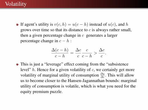
Volatility

If agent’s utility is v(c, h) = u(c− h) instead of u(c), and hgrows over time so that its distance to c is always rather small,then a given percentage change in c generates a largerpercentage change in c− h :

∆(c− h)

c− h=

∆c

c

c

c− h>

∆c

c.

This is just a “leverage” effect coming from the “subsistencelevel” h. Hence for a given volatility of c, we certainly get morevolatility of marginal utility of consumption ∂u

∂c . This will allowus to become closer to the Hansen-Jagannathan bounds: marginalutility of consumption is volatile, which is what you need for theequity premium puzzle.

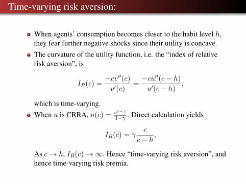
Time-varying risk aversion:

When agents’ consumption becomes closer to the habit level h,they fear further negative shocks since their utility is concave.

The curvature of the utility function, i.e. the “index of relativerisk aversion”, is

IR(c) =−cv′′(c)v′(c)

=−cu′′(c− h)

u′(c− h),

which is time-varying.

When u is CRRA, u(c) = c1−γ

1−γ . Direct calculation yields

IR(c) = γc

c− h,

As c→ h, IR(c)→∞. Hence “time-varying risk aversion”, andhence time-varying risk premia.

Multiplicative habits

Utility:

E0

∞∑t=0

βt(Ct/Xt)

1−γ − 1

1− γ,

Assume habit is external then

Mt+1 =

(Ct+1

Ct

)−γ ( Xt

Xt+1

)γ−1

Assume one lag for simplicity:

Xt = Cκt−1

then

Mt+1 =

(Ct+1

Ct

)−γ (Ct−1

Ct

)κ(γ−1)

Implications:

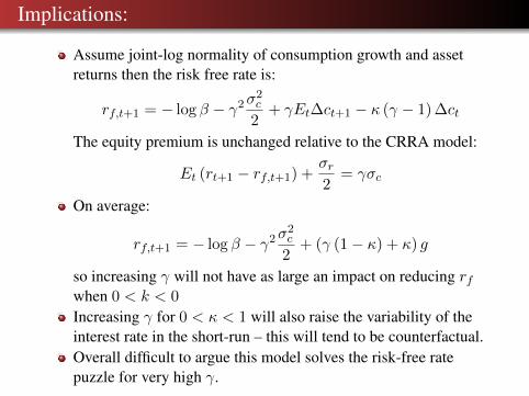
Assume joint-log normality of consumption growth and assetreturns then the risk free rate is:

rf,t+1 = − log β − γ2σ2c

2+ γEt∆ct+1 − κ (γ − 1) ∆ct

The equity premium is unchanged relative to the CRRA model:

Et (rt+1 − rf,t+1) +σr2

= γσc

On average:

rf,t+1 = − log β − γ2σ2c

2+ (γ (1− κ) + κ) g

so increasing γ will not have as large an impact on reducing rfwhen 0 < k < 0

Increasing γ for 0 < κ < 1 will also raise the variability of theinterest rate in the short-run – this will tend to be counterfactual.Overall difficult to argue this model solves the risk-free ratepuzzle for very high γ.

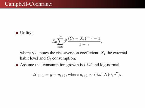
Campbell-Cochrane:

Utility:

E0

∞∑t=0

βt(Ct −Xt)

1−γ − 1

1− γ,

where γ denotes the risk-aversion coefficient, Xt the externalhabit level and Ct consumption.

Assume that consumption growth is i.i.d and log-normal:

∆ct+1 = g + ut+1, where ut+1 ∼ i.i.d. N(0, σ2).

Surplus consumption ratio:

Define the surplus consumption ratio St ≡ (Ct −Xt)/Ct. Notethat 0 < St < 1.

Assume that st = log(St) is related to consumption through thefollowing heteroskedastic AR(1) process:

st+1 = (1− φ)s+ φst + λ(st)(∆ct+1 − g).

This is a generalization of a standard AR(1), i.e.Xt = (1− δ)Xt−1 + Ct−1. The function λ(.) introduces anonlinearity, which will prove important.

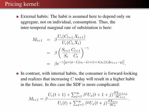
Pricing kernel:

External habits: The habit is assumed here to depend only onaggregate, not on individual, consumption. Thus, theinter-temporal marginal rate of substitution is here:

Mt+1 = βUc(Ct+1,Xt+1)

Uc(Ct,Xt)

= β

(St+1

St

Ct+1

Ct

)−γ= βe−γ[g+(φ−1)(st−s)+(1+λ(st))(∆ct+1−g)].

In contrast, with internal habits, the consumer is forward-lookingand realizes that increasing C today will result in a higher habitin the future. In this case the SDF is more complicated:

Mt+1 = βUc(t+ 1) +

∑∞j=1 β

jUx(t+ 1 + j)∂Xt+1+j

∂Ct+1

Uc(t) +∑∞

j=1 βjUx(t+ j)

∂Xt+j∂Ct

.

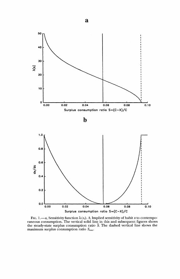
Sensitivity function:

Campbell and Cochrane use the following sensitivity function:

λ(st) =1

S

√1− 2(st − s)− 1, when s ≤ smax, 0 elsewhere,

where S and smax are respectively the steady-state and upperbound of the surplus-consumption ratio, which we set as:

S = σ

√γ

1− φ,

and

smax = s+1− S2

2.

These two values for S and smax are one possible choice, whichthey justify to make the habit locally predetermined.

Risk free rate:

This sensitivity function allows them to have a constant risk-freeinterest rate. To see this, note that the risk-free rate is

rft+1 = − log β + γg − γ(1− φ)(st − s)−γ2σ2

2(1 + λ(st))

2 .

Two effects where st appears: intertemporal substitution andprecautionary savings. When st is low, households have a lowIES which drives the risk free rate up. High risk aversion inducesmore precautionary savings which drives the risk free rate down.

CC offset these two effects by picking λ such that

γ(1− φ)(st − s) +γ2σ2

2(1 + λ(st))

2 = constant.

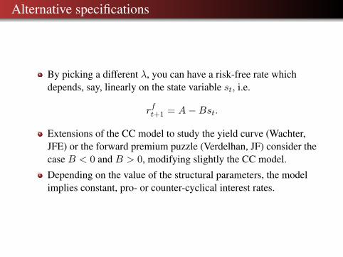
Alternative specifications

By picking a different λ, you can have a risk-free rate whichdepends, say, linearly on the state variable st, i.e.

rft+1 = A−Bst.

Extensions of the CC model to study the yield curve (Wachter,JFE) or the forward premium puzzle (Verdelhan, JF) consider thecase B < 0 and B > 0, modifying slightly the CC model.

Depending on the value of the structural parameters, the modelimplies constant, pro- or counter-cyclical interest rates.

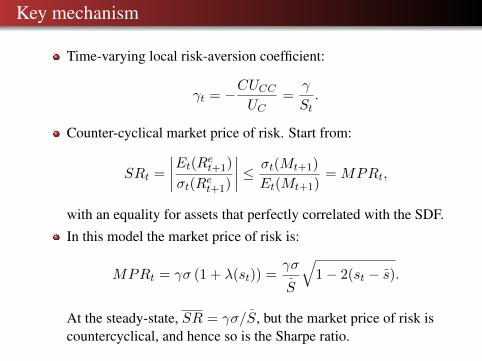
Key mechanism

Time-varying local risk-aversion coefficient:

γt = −CUCCUC

=γ

St.

Counter-cyclical market price of risk. Start from:

SRt =

∣∣∣∣Et(Ret+1)

σt(Ret+1)

∣∣∣∣ ≤ σt(Mt+1)

Et(Mt+1)= MPRt,

with an equality for assets that perfectly correlated with the SDF.

In this model the market price of risk is:

MPRt = γσ (1 + λ(st)) =γσ

S

√1− 2(st − s).

At the steady-state, SR = γσ/S, but the market price of risk iscountercyclical, and hence so is the Sharpe ratio.

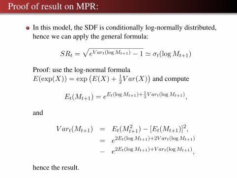
Proof of result on MPR:

In this model, the SDF is conditionally log-normally distributed,hence we can apply the general formula:

SRt =√eV art(logMt+1) − 1 ' σt(logMt+1)

Proof: use the log-normal formulaE(exp(X)) = exp

(E(X) + 1

2V ar(X))

and compute

Et(Mt+1) = eEt(logMt+1)+ 12V art(logMt+1),

and

V art(Mt+1) = Et(M2t+1)− [Et(Mt+1)]2,

= e2Et(logMt+1)+2V art(logMt+1)

− e2Et(logMt+1)+V art(logMt+1),

hence the result.

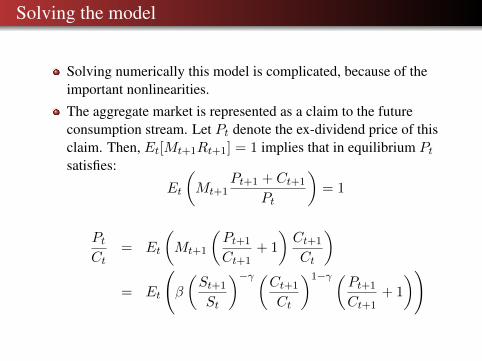
Solving the model

Solving numerically this model is complicated, because of theimportant nonlinearities.

The aggregate market is represented as a claim to the futureconsumption stream. Let Pt denote the ex-dividend price of thisclaim. Then, Et[Mt+1Rt+1] = 1 implies that in equilibrium Ptsatisfies:

Et

(Mt+1

Pt+1 + Ct+1

Pt

)= 1

PtCt

= Et

(Mt+1

(Pt+1

Ct+1+ 1

)Ct+1

Ct

)= Et

(β

(St+1

St

)−γ (Ct+1

Ct

)1−γ (Pt+1

Ct+1+ 1

))

Solution:

The state variable is st.

We solve for a fixed point, i.e. PtCt

= h(st) with

h(st) = Eut+1

(β

(St+1

St

)−γ (Ct+1

Ct

)1−γ(h(st+1) + 1)

),

with∆ct+1 = g + ut+1,

st+1 = (1− φ)s+ φst + λ(st)ut+1,

ut+1 ∼ i.i.d.N(0, σ2).

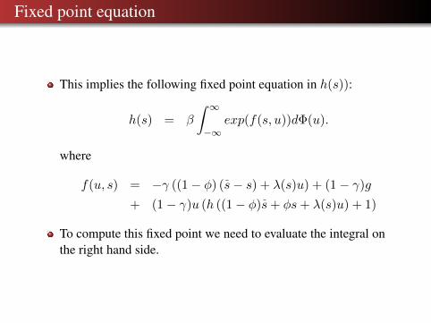
Fixed point equation

This implies the following fixed point equation in h(s)):

h(s) = β

∫ ∞−∞

exp(f(s, u))dΦ(u).

where

f(u, s) = −γ ((1− φ) (s− s) + λ(s)u) + (1− γ)g

+ (1− γ)u (h ((1− φ)s+ φs+ λ(s)u) + 1)

To compute this fixed point we need to evaluate the integral onthe right hand side.

Recipe:

Set a grid for s, {s1, s2, ..., sN} ;

Take a guess for h, i.e. {h (s1) , h (s2) , ..., h (sN )} ;

For each value of s in the grid, compute the RHS of thefixed-point equation numerically. We need to interpolate h tofind its value at the point (1− φ)s+ φs+ λ(s)u since it liesoutside the grid.

To compute the integral numerically, one way is to use aquadrature, e.g.

∫k(u)du =

∑i ωik(ui) for some points ui.

This gives a new guess for h using the fixed-point equation. Wekeep iterating on this equation until convergence.

Once we know h, we have the P-D ratio and the rest can becomputed simply, as in Mehra-Prescott. (See Wachter, Financeresearch letters, for a note detailing the computation of thatmodel.)

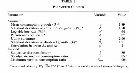
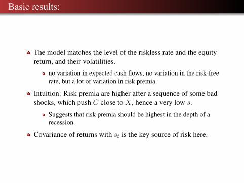
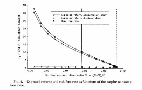
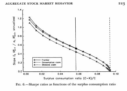
Basic results:

The model matches the level of the riskless rate and the equityreturn, and their volatilities.

no variation in expected cash flows, no variation in the risk-freerate, but a lot of variation in risk premia.

Intuition: Risk premia are higher after a sequence of some badshocks, which push C close to X , hence a very low s.

Suggests that risk premia should be highest in the depth of arecession.

Covariance of returns with st is the key source of risk here.

Additional results:

Volatility of returns is higher in bad times.

The model also matches the time-series predictability evidence:dividend growth is not predictable, but returns are predictable,and the volatility of the P-D ratio is accounted for by this latterterm (“discount rate news”).

Long-run equity premium: because of mean-reversion in stockprices, excess returns on stocks at long horizons are even morepuzzling than the standard one-period ahead puzzle. CC notethat if the state variable is stationary, the long-run standarddeviation of the SDF will not depend on the current state. Keypoint: in their model, S−γ is not stationary – variance is growingwith horizon!