BANK OF GREECE

EUROSYSTEM

Working PaperThe effect of asset price volatility

on fiscal policy outcomes

Athanasios Tagkalakis

WORKINKPAPERWORKINKPAPERWORKINKPAPERWORKINKPAPERWORKINKPAPERNOVEMBER 2009

106

BANK OF GREECE Economic Research Department – Special Studies Division 21, Ε. Venizelos Avenue GR-102 50 Athens Τel: +30210-320 3610 Fax: +30210-320 2432 www.bankofgreece.gr Printed in Athens, Greece at the Bank of Greece Printing Works. All rights reserved. Reproduction for educational and non-commercial purposes is permitted provided that the source is acknowledged. ISSN 1109-669

THE EFFECT OF ASSET PRICE VOLATILITY ON FISCAL POLICY OUTCOMES

Athanasios Tagkalakis Bank of Greece

ABSTRACT This paper examines the effect of asset price volatility on fiscal policy stance. We find that asset price volatility affects the volatility of discretionary fiscal policy in a positive and significant manner, which according to Fatas and Mihov (2003) has negative repercussions on output volatility and economic growth. Higher residential property price volatility amplifies both the volatility of government spending and the volatility of the discretionary fiscal policy stance. Equity price volatility increases the volatility of the fiscal policy stance, primarily via the government revenue channel. Keywords: Asset prices, fiscal policy, volatility. JEL classification: E61, E62, H61, H62, E32 Acknowledgements: I would like to thank the BIS for kindly providing the asset price data. I would also like to thank Christos Antonopoulos, Fragiskos Archontakis, Michael Artis, Claudio Borio, Heather Gibson, Panagiotis Konstantinou, Ludger Schuknecht, Pantelis Tagkalakis, Joel Slemrod and Jose Tavares. The views of the paper are my own and do not necessarily reflect those of the Bank of Greece. Correspondence: Athanasios Tagkalakis Economic Research Department, Bank of Greece, 21 E. Venizelos Ave., 10250 Athens, Greece Tel.:+30-210-320 2442 Email: atagkalakis@bankofgreece.gr

4

1. Introduction

The on-going economic and financial market turmoil has been accompanied by a

significant fall in asset prices, following several years of asset price boom. These asset

price movements affect the fiscal policy stance through a series of channels (see e.g.,

Schuknecht and Eschenbach, 2004). Directly, they affect specific revenue categories, e.g.,

capital gains and losses related to direct taxes on households and businesses. Indirectly,

they affect revenue via a feedback loop from higher asset prices to real economic activity

(higher asset prices raise consumer confidence and consumption, via the wealth effect,)

which increases the collection of indirect taxes. Finally, in case asset price busts lead to

defaults of financial institutions, the state will be asked to intervene to preserve the

stability of the financial system.

This paper goes beyond the previous literature in examining whether asset price

volatility amplifies the volatility of fiscal policy outcomes, which according to Fatas and

Mihov (2003) has negative repercussions on output volatility and economic growth.1

Following previous studies, e.g., Jaeger and Schuknecht (2004) we use a real aggregate

asset price index (taken from the Bank of International Settlements-BIS; see Appendix).

2. Asset price volatility and fiscal policy

Using data for 17 OECD countries for the period 1970 to 2005, we find

preliminary evidence that asset price volatility has been increasing over time.2 Driven by

this evidence, we examine whether this had any significant impact on the volatility of

fiscal policy stance, as measured by the standard deviation of the change in the cyclically

adjusted primary balance as a percent of GDP. Next, we repeat the same exercise for the

volatility of government spending and government revenue, as measured, respectively, by 1 According to Fatas and Mihov (2003) the volatility of output caused by discretionary fiscal policy lowers economic growth by more than 0.8 percentage points for every percentage point increase in volatility 2 While the volatility of economic activity cycles has fallen over the time (either due to better policies or to smaller shocks), the volatility of aggregate asset price movements appears to have increased. Splitting the sample into four sub-samples we see that the standard deviation of the output gap (real GDP growth) was 1.946 (0.025) in 1970-1979, 2.389 (0.018) in 1980-1989, 2.635 (0.025) in 1990-1999 and 1.508 (0.015) in 2000-2005, i.e. the volatility of economic activity has gradually declined over the time. However, in the case of the change in the aggregate asset price series, the standard deviation was 0.081 in 1970-79, 0.084 in 1980-89, 0.088 in 1990-99 and 0.141 in 2000-2005, i.e., it has been increasing.

5

the standard deviation of the change in the cyclically adjusted total expenditures

excluding interest payments as a percent of GDP, and the standard deviation of the

change in the cyclically adjusted total revenues as a percent of GDP.

Given that our analysis involves only 17 countries, we split the sample into four

parts, 1970-1979, 1980-1989, 1990-1999 and 2000-2005 and construct volatility

measures and average values for the respective variables and sub-samples. Therefore, our

unbalanced panel involves at the maximum 68 observations.

The dependent variable is the log of the standard deviation of the change in the

cyclically adjusted primary balance as a percent of GDP. The key explanatory variables

are the log of the standard deviation of the change in aggregate asset prices and the log of

the standard deviation of the real GDP growth. In principle, one could expect (as in Gali

and Perotti, 2003) that a fiscal policy rule implies that the fiscal stance, i.e. a measure of

discretionary fiscal policy making (e.g., the change in the cyclically adjusted primary

balance as a percent of GDP), would react to output deviations from trend (or

alternatively GDP growth). Hence, the fiscal policy maker can respond in a counter-

cyclical or pro-cyclical manner to output growth movements; this implies that the

volatility of real GDP growth should be taken on board when examining the determinants

of the volatility of the discretionary fiscal policy stance. Note that the sign of coefficient

can be either positive or negative, depending on whether the fiscal policy maker responds

in a very pronounced manner or not. In a similar manner a fiscal policy maker might be

asked to respond or take on board asset price movements. For example, this can happen

when a fiscal policy maker has to respond to an asset price bust by increasing government

spending in order to counterbalance the effects of falling asset prices on economic

activity and, possibly to address the related vulnerabilities of the financial system (see

Tagkalakis, 2009). Alternatively, if primary balances and in particular government

revenues are not adjusted both for the economic and the asset price cycle, then cyclically

adjusted primary balances (and cyclically adjusted revenues) will be affected by asset

price movements (see e.g., Jaeger and Schuknecht, 2004 and Morris and Schucknecht,

2007). Hence, asset price volatility should be taken on board when investigating the

determinants of the volatility of the fiscal policy stance. Note that the sign of the

coefficient of the asset price volatility variable can be either positive or negative.

6

An alternative formulation involves the logs of the standard deviation of the

disaggregated asset prices series, i.e., the change in real commercial property, real

residential property and real equity prices. The additional control variables used are the

average value of the cyclically adjusted primary balance as a percent of GDP and the

average value of the debt ratio. These variables control for the initial budgetary

conditions. An alternative specification includes the average value of the cyclically

adjusted total expenditures excluding interest payments as a percent of GDP and controls

for the government size and the role that the government might have in stabilizing the

economy via discretionary fiscal policy (see Gali, 1994; Fatas and Mihov, 2003).

Following Rodrick (1998) and Fatas and Mihov (2003) we include the ratio of imports

and exports as a percent to GDP (Trade) to control for the fact that a higher degree of

openness might induce governments to use more actively fiscal policy in order to

stabilize their economies. Finally, we include the real short term interest rate (RIRS) to

control for monetary conditions.

The government spending and revenue specifications include, respectively, the

average values of the cyclically adjusted total expenditures excluding interest payments

as a percent of GDP and the cyclically adjusted total revenues as a percent of GDP.

Two specifications are considered each time, one with the contemporaneous value

of the volatility of real GDP growth and a second where we instrument the

contemporaneous volatility of real GDP growth with its lagged value and the lagged

value of the standard deviation of output gap. The second specification controls for the

fact that some of the variation in the volatility of the cyclically adjusted fiscal policy

variable might still be due to output volatility and not to discretionary policy.

The results presented in Table 1 indicate that higher asset price volatility

translates into higher volatility of discretionary fiscal policy. Since both variables are in

logs, the coefficients report the elasticity of the volatility of discretionary policy with

respect to the asset price. A 1 percent increase in aggregate asset price volatility leads to a

0.16-0.27 percent increase in the volatility of discretionary fiscal policy.3 This finding is

3 According to Fatas and Mihov (2003) the volatility of output caused by discretionary fiscal policy lowers economic growth by more than 0.8 percentage points for every percentage point increase in volatility. Taking the findings by Fatas and Mihov (2003) at face value, a 1 percent increase in aggregate asset price

7

reaffirmed in Table 2 in the case of residential property and equity prices, with the effect

of the volatility of residential property prices being more significant (a 1 percent increase

in residential property price volatility leads to a 0.15-0.22 percent increase in the

volatility of discretionary fiscal policy). On the other hand, real commercial prices have a

negative, but insignificant, coefficient estimate. Moreover, an increase in output volatility

has no significant effect on the volatility of discretionary fiscal policy.

Turning to the other control variables, we see there is significant evidence that

openness, and higher interest rates increase the volatility of fiscal policy (Tables 1 and 2).

Higher primary surpluses or lower deficits lead to less volatile fiscal policy outcomes

(Tables 1 and 2). The proxy of government size enters with a positive coefficient (but is

significant only in Table 2), implying that larger governments use fiscal policy more

actively for stabilizing purposes and, thus, more volatile discretionary fiscal policy

outcomes.

As reported in Tables 3 and 4, there is evidence at the disaggregated level that

higher volatility in real residential property prices induces more volatile government

spending outcomes (a 1 percent increase in residential property price volatility leads to

about 0.22 percent increase in the volatility of government spending), while there is much

weaker evidence in the case of government revenues.4 Increased equity price volatility

amplifies the volatility of government revenues; a 1 percent increase in equity price

volatility leads to about 0.37 increase in the volatility of government revenues. Output

volatility has a positive effect on the volatility fiscal policy, though the effect is not

significant. The bigger the government size the more volatile government spending is,

which implies a more active stabilizing role for fiscal policy. More open economies have

volatility leads to a 0.16-0.27 percent increase in the volatility of discretionary fiscal policy, which then increases output volatility and consequently reduces economic growth by 0.13-0.22 percentage points. 4 This might be a bit odd given that one might expect that residential property prices affect mostly government revenues. However, as has been shown by Schuknecht and Eschenbach (2004) and Tagkalakis (2009) abrupt asset price movements (busts) linked with financial instability can lead to higher government spending. This will be the case when the government has to bear part of the burden of a private sector bailout or when it wants to take discretionary action in order to avert a negative feedback loop on economic activity which could lead to a full blown recession. Moreover, according to a recent European Commission (2009) study which investigates the fiscal costs of financial crisis, the deterioration of fiscal balances in past financial crises came primarily through the expenditure side, while revenue ratios were on average less affected.

8

to cope with more volatile government revenues. Finally, there is some evidence that a

higher debt ratio is linked with less volatile government spending.

3. Conclusions

Based on the fact that asset prices are particularly volatile, we found that there is

significant evidence that asset price volatility affects the volatility of discretionary fiscal

policy in a positive and significant manner. Higher residential property price volatility

leads to more volatile government spending and, thus, to more volatile discretionary

fiscal policy stance. Equity price volatility affects the volatility of the fiscal policy stance

primarily via the government revenue channel. On the other hand, output volatility has no

particular effect on the volatility of fiscal policy stance. Openness and the size of

government affect positively and significantly the volatility of discretionary fiscal policy;

the first, primarily, through the revenue channel and the second through government

spending.

Hence, fiscal policy makers should take into account asset price movements

because they amplify the volatility of discretionary fiscal policy stance. This would imply

that if primary balances and in particular government revenues are not adjusted for both

the economic and the asset price cycle, then cyclically adjusted primary balances (and

cyclically adjusted revenues) will be affected by asset price movements (see e.g., Jaeger

and Schuknecht, 2004 and Morris and Schucknecht, 2007). As a consequence the fiscal

policy maker will not have a clear grasp of developments in the fiscal policy stance. This

points to the need for adjusting fiscal balances, and in particular government revenues,

for asset price changes.

Given that asset price movements amplify the volatility of the discretionary fiscal

policy stance, which in turn amplifies business cycle fluctuations and harms economic

growth (Fatas and Mihov, 2003), a word of caution is needed as regards the fiscal policy

interventions undertaken (and their likely continuation) in response to the on-going

economic and financial market turmoil.

9

Fiscal policy makers should bear in mind, when asked to respond to abrupt asset

price movements (e.g., an asset price bust) and to address the likely implications for the

stability of the financial system (see Schuknecht and Eschenbach, 2004; Tagkalakis,

2009), that, while their intervention will most likely have a positive first order effect (in

terms of safeguarding or restoring economic and financial stability), it will also entail the

risk of increasing fiscal policy and, consequently, output volatility generating a negative

effect on economic growth, thus, putting a toll on economic recovery. This negative

effect should be perceived as an additional argument in favour of promptly withdrawing

the fiscal measures taken as a response to the economic and financial crisis when the

recovery gathers pace.

10

References European Commission, 2007. Ameco database. Retrieved from http://ec.europa.eu/economy_finance/indicators/annual_macro_economic_database/ameco_en.htm. European Commission, 2009. Public Finances in EMU. European Economy No 5. European Commission: Brussels.

Fatas, A., Mihov, I., 2003. The case for restricting fiscal policy discretion. Quarterly Journal of Economics 118, 1419-1447.

Gali, J., 1994. Government size and macroeconomic stability. European Economic Review 28, 117-132.

Gali, J., Perotti, R., 2003. Fiscal policy and monetary integration in Europe. Economic Policy 18, 533-572.

Jaeger, A., Schuknecht, L., 2004. Boom-bust phases in asset prices and fiscal policy behavior. IMF Working paper. No. 54.

Morris, R. & Schucknecht, L. (2007). Structural balances and revenue windfalls: The

role of asset prices. ECB Working paper. No 737.

Organization of Economic Cooperation and Development, (2007). Economic Outlook. (Paris: OECD).

Rodrick, D., 1998. Why do more open economic have bigger governments”. Journal of Political Economy 106, 997-1032.

Schuknecht, L., Eschenbanch, F., 2004. The fiscal costs of financial instability revisited. Economic Policy 14, 313-346. Tagkalakis, A. 2009. Fiscal policy rules and asset price movements, unpublished manuscript

11

Appendix Data

We used a yearly unbalanced panel data set (1970-2005) of 17 OECD economies:

Australia, Belgium, Canada, Germany, Denmark, Spain, Finland, France, United

Kingdom, Ireland, Italy, Japan, Netherlands, Norway, New Zealand, Sweden, and United

States.

Macroeconomic variables

The macroeconomic variables used extend from 1970 to 2005. Fiscal and output

variables are from the OECD Economic Outlook (2007), the definitions used are: the

lagged value of the cyclically adjusted primary balance as a percent of GDP (CAPBY),

the change in the cyclically adjusted primary balance as a percent of GDP (DCAPBY),

the lagged value of the debt to GDP ratio (Debt), the lagged value of the output gap

(Output gap), the lagged value of the short term real interest rate (RIRS), the change in

the primary balance as a share of GDP (Change in primary balance), the change in

cyclically adjusted total expenditure excluding interest payments as a share of GDP

(DCATDXY), cyclically adjusted total expenditure excluding interest payments as a

share of GDP (CATDXY), the change in cyclically adjusted total revenues as a share of

GDP (DCATRY), cyclically adjusted total revenues as a share of GDP (CATRY). We

also used the real GDP growth rate and an openness index (TRADE) which was

constructed as the ratio of imports plus exports to GDP.

Asset price variables

The main indicator is the change in the log of the annual aggregate real asset

prices (DRAAP), which covers 1970-2005 for 17 industrial countries and combines price

indices for three asset classes - equities, residential property and commercial property –

by weighting the components using shares of the asset classes in private sector wealth.

The private consumption deflator is used to convert nominal to real asset prices. In

addition, we considered also the change in the log of the three disaggregate asset price

indices, i.e., real commercial prices (DRCP), real residential prices (DRRP) and real

equity prices (DREP).

12

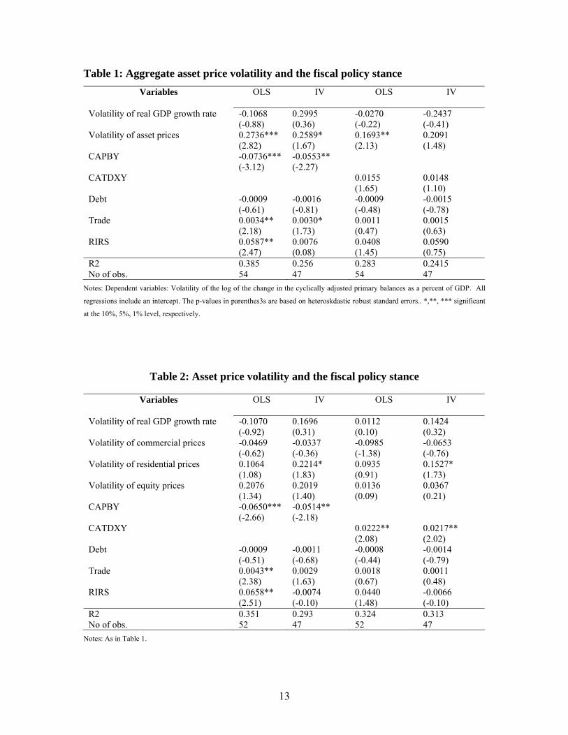
Table 1: Aggregate asset price volatility and the fiscal policy stance Variables OLS IV OLS

IV

Volatility of real GDP growth rate -0.1068 (-0.88)

0.2995 (0.36)

-0.0270 (-0.22)

-0.2437 (-0.41)

Volatility of asset prices 0.2736*** (2.82)

0.2589* (1.67)

0.1693** (2.13)

0.2091 (1.48)

CAPBY -0.0736*** (-3.12)

-0.0553** (-2.27)

CATDXY 0.0155 (1.65)

0.0148 (1.10)

Debt -0.0009 (-0.61)

-0.0016 (-0.81)

-0.0009 (-0.48)

-0.0015 (-0.78)

Trade 0.0034** (2.18)

0.0030* (1.73)

0.0011 (0.47)

0.0015 (0.63)

RIRS 0.0587** (2.47)

0.0076 (0.08)

0.0408 (1.45)

0.0590 (0.75)

R2 0.385 0.256 0.283 0.2415 No of obs. 54 47 54 47

Notes: Dependent variables: Volatility of the log of the change in the cyclically adjusted primary balances as a percent of GDP. All

regressions include an intercept. The p-values in parenthes3s are based on heteroskdastic robust standard errors.. *,**, *** significant

at the 10%, 5%, 1% level, respectively.

Table 2: Asset price volatility and the fiscal policy stance

Variables OLS IV OLS

IV

Volatility of real GDP growth rate -0.1070 (-0.92)

0.1696 (0.31)

0.0112 (0.10)

0.1424 (0.32)

Volatility of commercial prices -0.0469 (-0.62)

-0.0337 (-0.36)

-0.0985 (-1.38)

-0.0653 (-0.76)

Volatility of residential prices 0.1064 (1.08)

0.2214* (1.83)

0.0935 (0.91)

0.1527* (1.73)

Volatility of equity prices 0.2076 (1.34)

0.2019 (1.40)

0.0136 (0.09)

0.0367 (0.21)

CAPBY -0.0650*** (-2.66)

-0.0514** (-2.18)

CATDXY 0.0222** (2.08)

0.0217** (2.02)

Debt -0.0009 (-0.51)

-0.0011 (-0.68)

-0.0008 (-0.44)

-0.0014 (-0.79)

Trade 0.0043** (2.38)

0.0029 (1.63)

0.0018 (0.67)

0.0011 (0.48)

RIRS 0.0658** (2.51)

-0.0074 (-0.10)

0.0440 (1.48)

-0.0066 (-0.10)

R2 0.351 0.293 0.324 0.313 No of obs. 52 47 52 47

Notes: As in Table 1.

13

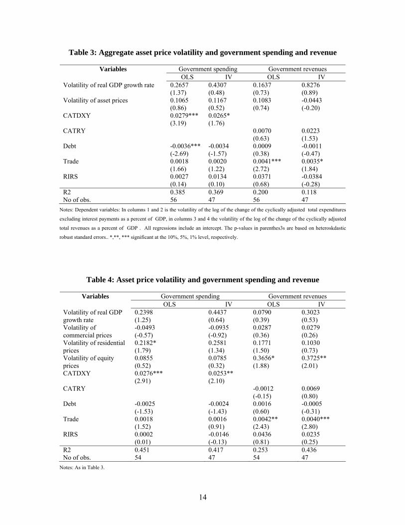
Table 3: Aggregate asset price volatility and government spending and revenue

Government spending Government revenues Variables OLS IV OLS IV

Volatility of real GDP growth rate 0.2657 (1.37)

0.4307 (0.48)

0.1637 (0.73)

0.8276 (0.89)

Volatility of asset prices 0.1065 (0.86)

0.1167 (0.52)

0.1083 (0.74)

-0.0443 (-0.20)

CATDXY 0.0279*** (3.19)

0.0265* (1.76)

CATRY 0.0070 (0.63)

0.0223 (1.53)

Debt -0.0036*** (-2.69)

-0.0034 (-1.57)

0.0009 (0.38)

-0.0011 (-0.47)

Trade 0.0018 (1.66)

0.0020 (1.22)

0.0041*** (2.72)

0.0035* (1.84)

RIRS 0.0027 (0.14)

0.0134 (0.10)

0.0371 (0.68)

-0.0384 (-0.28)

R2 0.385 0.369 0.200 0.118 No of obs. 56 47 56 47

Notes: Dependent variables: In columns 1 and 2 is the volatility of the log of the change of the cyclically adjusted total expenditures

excluding interest payments as a percent of GDP, in columns 3 and 4 the volatility of the log of the change of the cyclically adjusted

total revenues as a percent of GDP . All regressions include an intercept. The p-values in parenthes3s are based on heteroskdastic

robust standard errors.. *,**, *** significant at the 10%, 5%, 1% level, respectively.

Table 4: Asset price volatility and government spending and revenue

Government spending Government revenues Variables OLS IV OLS IV

Volatility of real GDP growth rate

0.2398 (1.25)

0.4437 (0.64)

0.0790 (0.39)

0.3023 (0.53)

Volatility of commercial prices

-0.0493 (-0.57)

-0.0935 (-0.92)

0.0287 (0.36)

0.0279 (0.26)

Volatility of residential prices

0.2182* (1.79)

0.2581 (1.34)

0.1771 (1.50)

0.1030 (0.73)

Volatility of equity prices

0.0855 (0.52)

0.0785 (0.32)

0.3656* (1.88)

0.3725** (2.01)

CATDXY 0.0276*** (2.91)

0.0253** (2.10)

CATRY -0.0012 (-0.15)

0.0069 (0.80)

Debt -0.0025 (-1.53)

-0.0024 (-1.43)

0.0016 (0.60)

-0.0005 (-0.31)

Trade 0.0018 (1.52)

0.0016 (0.91)

0.0042** (2.43)

0.0040*** (2.80)

RIRS 0.0002 (0.01)

-0.0146 (-0.13)

0.0436 (0.81)

0.0235 (0.25)

R2 0.451 0.417 0.253 0.436 No of obs. 54 47 54 47

Notes: As in Table 3.

14

BANK OF GREECE WORKING PAPERS

90. Tavlas, G., H. Dellas and A. Stockman, “The Classification and Performance of Alternative Exchange-Rate Systems”, September 2008.

91. Milionis, A. E. and E. Papanagiotou, “A Note on the Use of Moving Average

Trading Rules to Test for Weak Form Efficiency in Capital Markets”, October 2008.

92. Athanasoglou, P.P. E. A. Georgiou and C. C. Staikouras, “Assessing Output and

Productivity Growth in the Banking Industry”, November 2008. 93. Brissimis, S. N. and M. D. Delis, “Bank-Level Estimates of Market Power”,

January 2009. 94. Members of the SEEMHN Data Collection Task Force with a Foreword by Michael

Bordo and an introduction by Matthias Morys, “Monetary Time Series of Southeastern Europe from 1870s to 1914”, February 2009.

95. Chronis, P., “Modeling Distortionary Taxation”, March 2009. 96. Hondroyiannis, G., “Fertility Determinants and Economic Uncertainty: An

Assessment using European Panel Data”, April 2009 97. Papageorgiou, D., “Macroeconomic Implications of Alternative Tax Regimes: The

Case of Greece”, May 2009. 98. Zombanakis, G. A., C. Stylianou and A. S. Andreou, “The Greek Current Account

Deficit: Is It Sustainable After All?”, June 2009. 99. Sideris, D., “Optimum Currency Areas, Structural Changes and the Endogeneity of

the OCA Criteria: Evidence from Six New EU Member States”, July 2009.

100. Asimakopoulos, I. and P. Athanasoglou, “Revisiting the Merger and Acquisition Performance of European Banks”, August 2009.

101. Brissimis, N. S. and D. M. Delis, “Bank Heterogeneity and Monetary Policy

Transmission”, August 2009. 102. Dellas, H. and G. S. Tavlas, “An Optimum-Currency-Area Odyssey”, September

2009. 103. Georgoutsos, A. D. and P. M. Migiakis, “Benchmark “Bonds Interactions under

Regime Shifts”, September 2009. 104. Tagkalakis, A., “Fiscal Adjustments and Asset Price Movements”, October 2009.

15

105. Lazaretou, S., “Money Supply and Greek Historical Monetary Statistics: Definition,

Construction, Sources and Data”, November 2009.

16