Coloring simple hypergraphs

Alan Frieze∗ Dhruv Mubayi†

October 1, 2013

Abstract

Fix an integer k ≥ 3. A k-uniform hypergraph is simple if every two edges share at most

one vertex. We prove that there is a constant c depending only on k such that every simple

k-uniform hypergraph H with maximum degree ∆ has chromatic number satisfying

χ(H) < c

(∆

log ∆

) 1k−1

.

This implies a classical result of Ajtai-Komlos-Pintz-Spencer-Szemeredi and its strengthening

due to Duke-Lefmann-Rodl. The result is sharp apart from the constant c.

1 Introduction

Hypergraph coloring has been studied for almost 50 years, since Erdos’ seminal results on the

minimum number of edges in uniform hypergraphs that are not 2-colorable. Some of the major

tools in combinatorics have been developed to solve problems in this area, for example, the Local

Lemma and the nibble or semirandom method. Consequently, the subject enjoys a prominent place

among basic combinatorial questions.

Closely related to coloring problems are questions about the independence number of hypergraphs.

An easy extension of Turan’s graph theorem shows that a k-uniform hypergraph with n vertices

and average degree d has an independent set of size at least cn/d1/(k−1), where c depends only on

k. If we impose local constraints on the hypergraph, then this bound can be improved. An i-cycle

in a k-uniform hypergraph is a collection of i distinct edges spanned by at most i(k − 1) vertices.

∗Department of Mathematical Sciences, Carnegie Mellon University, Pittsburgh PA 15213. Supported in part by

NSF Grants DMS-0753472 and CCF-1013110†Department of Mathematics, Statistics, and Computer Science, University of Illinois, Chicago, IL 60607. Sup-

ported in part by NSF Grants DMS-0653946, 0969092, 1300138

Keywords: hypergraph coloring, semi-random method

2010 Mathematics Subject classification: 05C15, 05C65, 05D40

1

Say that a k-uniform hypergraph has girth at least g if it contains no i-cycles for 2 ≤ i < g. Call

a k-uniform hypergraph simple if it has girth at least 3. In other words, every two edges have at

most one vertex in common. Throughout this paper we will assume that k ≥ 3 is a fixed positive

integer.

Ajtai-Komlos-Pintz-Spencer-Szemeredi [2] proved the following fundamental result that strength-

ened the bound obtained by Turan’s theorem above.

Theorem 1 ([2]) Let H = (V,E) be a k-uniform hypergraph of girth at least 5 with maximum

degree ∆. Then it has an independent set of size at least

c n

(log ∆

∆

)1/(k−1)

where c depends only on k.

Spencer conjectured that Theorem 1 holds even for simple hypergraphs, and this was later proved

by Duke-Lefmann-Rodl [6]. Theorem 1 has proved to be a seminal result in combinatorics, with

many applications. Indeed, the result was first proved for k = 3 by Komlos-Pintz-Szemeredi [13]

to disprove the famous Heilbronn conjecture, that among every set of n points in the unit square,

there are three points that form a triangle whose area is at most O(1/n2). For applications of

Theorem 1 to coding theory or combinatorics, see [15] or [14], respectively.

The goal of this paper is to prove a result that is stronger than Theorem 1 (and also the accompa-

nying result of [6]). Since the proof of our result does not use Theorem 1, it gives an alternative

proof of all the applications of Theorem 1 as well. Our main result states not only that one can

find an independent set of the size guaranteed by Theorem 1, but also that the entire vertex set

can be partitioned into independent sets with the average size as in Theorem 1. Recall that the

chromatic number χ(H) of H is the minimum number of colors needed to color the vertex set so

that no edge is monochromatic.

Theorem 2 Fix k ≥ 3. Let H = (V,E) be a simple k-uniform hypergraph with maximum degree

∆. Then

χ(H) < c

(∆

log ∆

) 1k−1

where c depends only on k.

It is shown in [5] that Theorem 2 is sharp apart from the constant c. In order to prove Theorem

2 we will first prove the following slightly weaker result. A triangle in a k-uniform hypergraph is

a 3-cycle that contains no 2-cycle. In other words, it is a collection of three sets A,B,C such that

every two of these sets have intersection of size one, and A ∩B ∩ C = ∅.

2

Theorem 3 Fix k ≥ 3. Let H = (V,E) be a simple triangle-free k-uniform hypergraph with

maximum degree ∆. Then

χ(H) < c

(∆

log ∆

) 1k−1

,

where c depends only on k.

The proof of Theorem 3 rests on several major developments in probabilistic combinatorics over

the past 25 years. Our approach is inspired by Johansson’s breakthrough result on graph coloring,

which proved Theorem 3 for k = 2.

The proof technique, which has been termed the semi-random, or nibble method, was first used by

Rodl (inspired by earlier work in [2, 13]) to confirm the Erdos-Hanani conjecture about the existence

of asymptotically optimal designs. Subsequently, Kim [11] (see also Kahn [10]) proved Johansson’s

theorem for graphs with girth five and then Johansson proved his result. The approach used by

Johansson for the graph case is to iteratively color a small portion of the (currently uncolored)

vertices of the graph, record the fact that a color already used at v cannot be used in future on

the uncolored neighbors of v, and continue this process until the graph induced by the uncolored

vertices has small maximum degree. Once this has been achieved, the remaining uncolored vertices

are colored using a new set of colors by the greedy algorithm.

In principle our method is the same, but there are several difficulties we encounter. The first, and

most important, is that our coloring algorithm is not as simple. A proper coloring of a k-uniform

hypergraph allows as many as k − 1 vertices of an edge to have the same color, indeed, to obtain

optimal results one must permit this. To facilitate this, we introduce a collection of k− 1 different

hypergraphs at each stage of the algorithm whose edges keep track of coloring restrictions. Keeping

track of these hypergraphs requires controlling more parameters during the iteration and dealing

with some more lack of independence and this makes the proof more complicated.

In an earlier paper [8], we had carried out this program for k = 3. Several technical ideas incorpo-

rated in the current proof can be found there. Because the notation in [8] is slightly simpler than

that in the current paper, the reader interested in the technical details of our proof may want to

familiarize him or herself with [8] first (although this paper is entirely self contained).

The implication Theorem 3 implies Theorem 2 forms a much shorter (but still nontrivial) part of

this paper (See Section 2). Our proof uses a recent concentration result of Kim and Vu [12] together

with some additional ideas similar to those from Alon-Krivelevich-Sudakov [3]. The approach here

is to partition the vertex set of a given simple hypergraph into some number of parts, where the

hypergraph induced by each of the parts is triangle-free. Once this has been achieved, each of the

parts is colored using Theorem 3.

We end with a conjecture posed in [8], which states that we may replace the hypothesis “simple”

with something much weaker.

3

Conjecture 4 ([8]) Let F be a k-uniform hypergraph. There is a constant cF depending only on

F such that every F -free k-uniform hypergraph with maximum degree ∆ has chromatic number at

most cF (∆/ log ∆)1/(k−1).

Conjecture 4 appears to be out of reach using current methods. For example, the special case k = 2

and F = K4 remains open and would imply an old conjecture of [1].

Throughout this paper, we will assume that ∆ is sufficiently large that all implied inequalities hold

true. Any asymptotic notation is meant to be taken as ∆→∞.

2 Simple hypergraphs

In this section we will prove that Theorem 3 implies Theorem 2.

Let H = (V,E) be a simple k-uniform hypergraph. For v ∈ V let its neighbor set NH(v) be

defined by NH(v) = x : ∃S ∈ E s.t. v, x ⊂ S. Let dH(v) denote the degree of v so that

|NH(v)| = (k − 1)dH(v).

A pair x, y ∈ NH(v) is said to be covered if there exists S ∈ E that contains both x and y but

not v. Note that the assumption that H is simple implies that in this case no edge contains all of

v, x, y.

Recall that k is fixed. Let ε = ε(k) be a sufficiently small positive constant depending only on k.

Theorem 2 will follow from Theorem 3 and the following two lemmas:

Lemma 5 Fix k ≥ 3. Let H = (V,E) be a simple k-uniform hypergraph with maximum degree ∆.

Let m =⌈∆

23k−4

−ε⌉

. Then there exists a partition of V into subsets V1, V2, . . . , Vm such that each

induced subhypergraph Hi = H[Vi], i = 1, 2, . . . ,m has the following properties:

(a) The maximum degree ∆i of Hi satisfies ∆i ≤ 2∆/mk−1.

(b) If v ∈ Vi then its Hi-neighborhood Ni(v) contains at most k2∆2/m3k−4 covered pairs. (Here

we mean covered w.r.t. Hi).

Lemma 6 Fix k ≥ 3 and let δ be a sufficiently small positive constant depending on k. Let

L = (V,E) be a simple k-uniform hypergraph with maximum degree at most d. Suppose that each

vertex neighborhood NL(v) contains at most dδ covered pairs. Let ` = d1

k−1−δ. Then there exists a

partition of V into subsets W1,W2, . . . ,W`1 , `1 = O(`) such that for each 1 ≤ j ≤ `1, the hypergraph

Lj = L[Wj ] has the following properties:

(a) The maximum degree dj of Lj satisfies dj ≤ 2d/`k−1.

(b) Lj is triangle-free.

4

2.1 Proof of Theorem 2

Our proof can be thought of as a nibble argument, involving two iterations, given by Lemmas 5

and 6. Suppose that H is a simple k-uniform hypergraph with maximum degree ∆ and assume

that ∆ is sufficiently large. Apply Lemma 5 to obtain H1, . . . ,Hm that satisfy the conclusion of

the lemma. Now fix 1 ≤ i ≤ m and let L = Hi. Lemma 5 part (a) implies that ∆(L) ≤ 2∆/mk−1.

Hence we may apply Lemma 6 to L with d = 2∆/mk−1 and δ = ε(3k − 4)2/(k − 2). By Lemma 5

part (b), each neighborhood NL(v) contains at most k2∆2/m3k−4 covered pairs. Since ∆ is large,

k2 ∆2

m3k−4≤ k2∆ε(3k−4) = k2∆

δ(k−2)3k−4 < dδ.

We may therefore apply Lemma 6 with ` = d1/(k−1)−δ. Together with Theorem 3 we obtain

χ(L) ≤∑j=1

χ(Lj) < O

(`

(d/`k−1

log(d/`k−1)

) 1k−1

)= O

((d

log(d(k−1)δ)

) 1k−1

)= O

((d

log d

) 1k−1

).

Since this holds for each Hi we obtain,

χ(H) ≤m∑i=1

χ(Hi) < O

(m

(d

log d

) 1k−1

)= O

(m

(∆/mk−1

log(∆/mk−1)

) 1k−1

)= O

((∆

log ∆

) 1k−1

).

2.2 Kim-Vu concentration

We will need the following very useful concentration inequality (1) from Kim and Vu [12]: Let

Υ = (W,F ) be a hypergraph of rank s, meaning that each f ∈ F satisfies |f | ≤ s. Let

Z =∑f∈F

∏i∈f

zi

where the zi, i ∈ W are independent random variables taking values in [0, 1]. For A ⊆ W, |A| ≤ s

let

ZA =∑f∈Ff⊇A

∏i∈f\A

zi.

Let MA = E(ZA) and Mj = maxA,|A|≥jMA for j ≥ 0. There exist positive constants a = as and

b = bs such that for any λ > 0,

P(|Z − E(Z)| ≥ aλs√M0M1) ≤ b|W |s−1e−λ. (1)

5

2.3 Proof of Lemma 5

We will use the Local Lemma in the form below.

Theorem 7 (Local Lemma) Let A1, . . . ,An be events in an arbitrary probability space. Suppose

that each event Ai is mutually independent of a set of all the other events Aj but at most d, and

that P (Ai) < p for all 1 ≤ i ≤ n. If ep(d+1) < 1, then with positive probability, none of the events

Ai holds.

We will partition V randomly into m parts of size ∼ |V |/m and use the Local Lemma to show

the existence of a partition. We make the partition by assigning a random number in [m] to each

v ∈ V .

Fix v ∈ V . To simplify notation, condition on v ∈ V1. Let Av be the event that (a) fails at v i.e.

that v has degree greater than 2∆/mk−1 in the hypergraph H1.

Let Bv be the event that its neighborhood in H1 contains more than k2∆2/m3k−4 covered pairs.

Each of these events is mutually independent of a set of all other events but at most O(∆4). We

will show that

P(Av),P(Bv) = O(∆−5) and this is clearly sufficient for the application of the Local Lemma.

Let dv be the degree of v in H1. Then dv has a distribution that is dominated by the binomial

distribution Bin(∆, 1/mk−1). It follows from the Chernoff bounds that

P(dv ≥ 2∆/mk−1

)≤ e−∆/(3mk−1) = e−∆

k−23k−4

−(k−1)ε+o(1)

≤ ∆−5

and this disposes of Av.

Our goal now is to bound P(Bv). For a vertex x ∈ NH(v), let Tv(x) denote the unique (k − 1)-set

containing x such that Tv(x) ∪ v ∈ E. A covered pair x, y ∈ NH(v) will remain as a covered

pair in NH1(v) iff Sx,y = Tv(x) ∪ Tv(y) ∪ T ⊆ V1 where T is the unique (k − 2)-set such that

T ∪ x, y ∈ E. Let S1, S2, . . . , Sr, r ≤ (k − 1)2(

∆2

)be an enumeration of the (3k − 4)-tuples Sx,y

as x, y ranges over the covered pairs in NH(v).

We will use the concentration inequality (1). The edges of our hypergraph (W,F ) are S1, S2, . . . , Sr

and if x ∈ W then zx is an independent 0, 1 Bernoulli random variable with P(zx = 1) = 1/m.

Note that |W | ≤ k∆2.

Let Zv denote the number of covered pairs in NH1(v). There is a 1-1 correspondence between

covered pairs and the Si. Therefore

µ = E(Zv) =r

m3k−4≤ (k − 1)2∆2

2m3k−4. (2)

We now have to estimate M1.

6

For each set A ⊂W , let YA denote the number of edges of F containing A.

Claim. |YA| = O(∆) if |A| ≤ k − 1 and |YA| = O(1) if |A| ≥ k.

Proof. Suppose that A ⊂ S ∈ F . Then S can be written as Tv(x) ∪ Tv(y) ∪ T , for some

x, y ∈ NH(v). We will count the number of S containing A by the number of Tv(x)’s and T ’s.

First, the number of S where both Tv(x) and Tv(y) have a vertex in A is at most 5k4 by the

following argument. There are(|A|

2

)< 5k2 choices for the two intersection points, these points

uniquely determine Tv(x) and Tv(y), and there are at most |Tv(y)||Tv(x)| = (k − 1)2 possible

covered pairs, each of which determines T uniquely (if T exists).

Now suppose that A∩Tv(y) = ∅. If |A| ≥ k, then A must contain a vertex from T and a (different)

vertex from Tv(x). There are at most 9k2 choices for these two vertices. For each of these choices,

Tv(x) is determined uniquely. For each vertex in Tv(x) and the chosen vertex of T ∩ A, there is

at most one choice for T (since H is simple), hence the number of choices for T is at most k − 1.

Having chosen T , there are at most k − 1 choices for Tv(y). Altogether, there are at most 9k4

choices for S. We conclude that if |A| ≥ k, then

|YA| ≤ 5k4 + 9k4 = O(1).

If |A| ≤ k − 1, the argument above still applies unless either A ⊂ Tv(x) or A ⊂ T . In either case,

there are at most k∆ ways of choosing the other part of S \ Tv(y) and at most k ways of choosing

Tv(y). Thus |YA| = O(∆) as claimed.

The probability of choosing each vertex in S \ A is 1/m, so for given A, the probability of a

particular S ⊃ A is (1/m)3k−4−|A|. The Claim now implies that for 1 ≤ |A| < 3k − 4,

MA ≤ max

O

(∆

m2k−3

), O

(1

m

).

When |A| = 3k − 4 we have MA = 1. By our choice of m, it follows that if ε is sufficiently small

then

M1 = 1.

The choice of m also gives

M0 = maxµ, 1 ≤ k2∆2

m3k−4= k2∆(3k−4)ε.

It follows that if we take aλ3k−4 = k2∆2

2m3k−4(M0M1)1/2 then λ > ∆δk where δk > 0. Now (1) implies

that

P(Bv) ≤ P(Zv − E(Zv) ≥ k2∆2/2m3k−4) ≤ b(k∆2)3ke−λ ≤ ∆−5.

This completes the proof of Lemma 5.

7

2.4 Proof of Lemma 6

This part follows an approach taken in Alon, Krivelevich and Sudakov [3]. We will first partition V

randomly into ` parts V1, V2, . . . , V` of size ∼ |V |/` and use the local lemma to show the existence

of a partition satisfying certain properties. To simplify notation, condition on v ∈ V1.

For v ∈ V let Av be the event that (a) fails at v i.e. that v has degree greater than 2d/`k−1 in L1.

Let Bv be the event that NL1(v) contains at least 200k2 covered pairs w.r.t. L1.

Each of these events is mutually independent of a set of all other events but at most O(d4). We

will show that

P(Av),P(Bv) = O(d−5) and this is clearly sufficient for the application of the Local Lemma.

Let dv be the degree of v in L1. Then dv has a distribution that is dominated by the binomial

distribution Bin(d, 1/`k−1). It follows from the Chernoff bounds that

P(dv ≥ 2d/`k−1

)≤ e−d/(3`k−1) = e−d

(k−1)δ/3 ≤ d−5

and this disposes of the Av.

If Bv fails then either

(i) There exists a vertex w ∈ NL(v) such that w is in at least 10k covered pairs of NL1(v), or

(ii) NL1(v) contains at least 10k pair-wise disjoint covered pairs.

Now

P((i)) ≤ kd

(dδ

10k

)`−10k ≤ d−5

P((ii)) ≤(d2δ

10k

)`−20k ≤ d−5

and this disposes of the Bv.

So, assume that none of the events Av, Bv occur. We show now that we can partition each Vj into

at most 400k2 + 1 sets, each of which induces a triangle free hypergraph. Consider the digraph D1

with vertex set V1 and an edge directed from v ∈ V1 to each vertex of each of the at most 200k2

covered pairs in NL1(v). D1 has maximum out-degree 400k2 and so its underlying graph G1 is

400k2-degenerate and so it can be properly colored with 400k2 + 1 colors. Partition V1 into color

classes W1,W2, . . . ,W400k2+1. We claim that for each s, the hypergraph L[Ws] induced by Ws is

triangle-free. Suppose then that there is a triangle v ∪ Tv(x), v ∪ Tv(y), T inside L[Ws], where T

contains both x and y. Then x, y is a covered pair for v and by construction v and x are not in

the same Ws, contradiction.

8

3 Triangle-free hypergraphs

In this section, which forms the bulk of the paper, we will prove Theorem 3.

3.1 Local Lemma

The driving force of our upper bound argument, both in the semi-random phase and the final

phase, is the Local Lemma. Note that the Local Lemma immediately implies that every k-uniform

hypergraph with maximum degree ∆ can be properly colored with at most⌈4∆1/(k−1)

⌉colors.

Indeed, if we color each vertex randomly and independently with one of these colors, the probability

of the event Ae, that an edge e is monochromatic, is at most 14k−1∆

. Moreover Ae is independent

of all other events Af unless |f ∩ e| > 0, and the number of f satisfying this is less than k∆. We

conclude that there is a proper coloring.

3.2 Coloring Procedure

In the rest of the paper, we will prove the upper bound in Theorem 3. Suppose that k ≥ 3 is fixed

and H is a simple triangle-free k-uniform hypergraph with maximum degree ∆.

Let V be the vertex set of H. As usual, we write χ(H) for the chromatic number of H. Let ε be

a sufficiently small fixed positive constant (depending only on k). Let

ω =ε2 log ∆

100× k2k+1

and set

q =

⌈∆1/(k−1)

ω1/(k−1)

⌉.

Note that q < c(∆/ log ∆)1/(k−1) where c depends only on k.

We color V with 2q colors and therefore show that

χ(H) ≤ 2c

(∆

log ∆

)1/(k−1)

.

We use the first q colors to color H in rounds and then use the second q colors to color any vertices

not colored by this process.

Our algorithm for coloring in rounds is semi-random. At the beginning of a round certain param-

eters will satisfy certain properties, (9) – (14) below. We describe a set of random choices for the

parameters in the next round and we use the Local Lemma to prove that there is a set of choices

that preserves the required properties.

• C = [q] denotes the set of available colors for the semi-random phase.

9

• U (t): The set of vertices which are currently uncolored. (U (0) = V ).

• H(t): The sub-hypergraph of H induced by U (t).

• W (t) = V \U (t): The set of vertices that have been colored. We use the notation κ to denote

the color of an item e.g. κ(w), w ∈W (t) denotes the color permanently assigned to w.

• H(t)i , 2 ≤ i ≤ k − 1: An edge-colored i-graph with vertex set U (t). There is an edge

u1u2 · · ·ui ∈ H(t)i iff there are vertices ui+1, ui+2, . . . , uk ∈ W (t) and an edge u1u2 · · ·uk ∈ H

with κ(ui+1) = κ(ui+2) = · · · = κ(uk). The edge u1u2 · · ·ui is given the color κ(ui+1). For a

fixed u1u2 · · ·ui, this color is well defined because H is simple. (These hypergraphs are used

to keep track of coloring restrictions).

• p(t)u ∈ [0, 1]C for u ∈ U (t): This is a vector of coloring probabilities. The cth coordinate is

denoted by p(t)u (c) and p

(0)u = (q−1, q−1, . . . , q−1).

We can now describe the “algorithm” for computing U (t+1), H(t+1)i , p

(t+1)u , given U (t), H

(t)i , p

(t)u , for

u ∈ U (t): Let

θ =ε

ω=

100× k2k+1

ε log ∆

where we recall that ε is a sufficiently small positive constant.

For each u ∈ U (t) and c ∈ C we tentatively activate c at u with probability θp(t)u (c). A color c is

lost at u ∈ U (t), if either

(i) there is an edge uu2 · · ·uk ∈ H(t) such that c is tentatively activated at u2, u3, . . . , uk or

(ii) there is a 2 ≤ i ≤ k−1 and an edge e = uu2 · · ·ui ∈ H(t)i such that c = κ(e) and c is tentatively

activated at u2, u3, . . . , ui.

We fix

p =1

∆1/(k−1)−ε .

We keep

p(t)u (c) ≤ p

for all t, u, c.

We let

B(t)(u) =c : p(t)

u (c) = p

for all u ∈ V.

A color in B(t)(u) will not be used at u. The role of B(t)(u) is clarified in Section 3.3.

The vertex u ∈ U (t) is given a permanent color if there is a color tentatively activated at u which

is not lost due to (i) or (ii) and not in B(t)(u). If there is a choice, it is made arbitrarily. Then u

is placed into W (t+1).

10

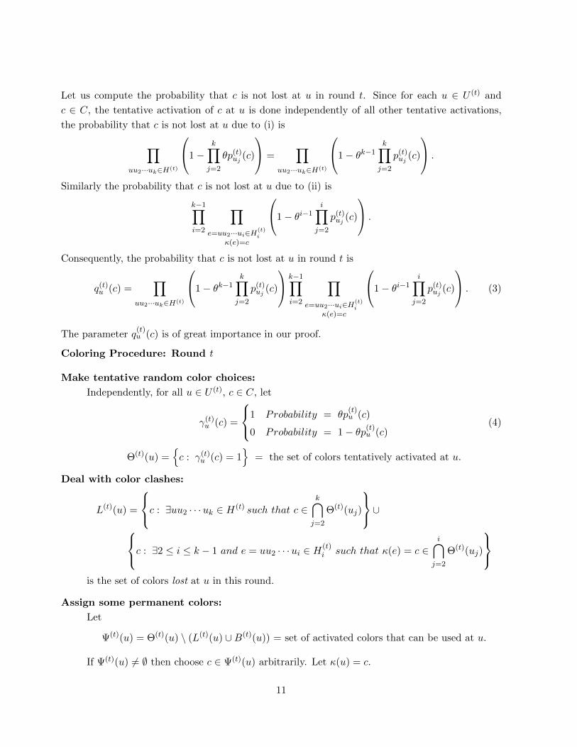
Let us compute the probability that c is not lost at u in round t. Since for each u ∈ U (t) and

c ∈ C, the tentative activation of c at u is done independently of all other tentative activations,

the probability that c is not lost at u due to (i) is

∏uu2···uk∈H(t)

1−k∏j=2

θp(t)uj (c)

=∏

uu2···uk∈H(t)

1− θk−1k∏j=2

p(t)uj (c)

.

Similarly the probability that c is not lost at u due to (ii) is

k−1∏i=2

∏e=uu2···ui∈H

(t)i

κ(e)=c

1− θi−1i∏

j=2

p(t)uj (c)

.

Consequently, the probability that c is not lost at u in round t is

q(t)u (c) =

∏uu2···uk∈H(t)

1− θk−1k∏j=2

p(t)uj (c)

k−1∏i=2

∏e=uu2···ui∈H

(t)i

κ(e)=c

1− θi−1i∏

j=2

p(t)uj (c)

. (3)

The parameter q(t)u (c) is of great importance in our proof.

Coloring Procedure: Round t

Make tentative random color choices:

Independently, for all u ∈ U (t), c ∈ C, let

γ(t)u (c) =

1 Probability = θp(t)u (c)

0 Probability = 1− θp(t)u (c)

(4)

Θ(t)(u) =c : γ(t)

u (c) = 1

= the set of colors tentatively activated at u.

Deal with color clashes:

L(t)(u) =

c : ∃uu2 · · ·uk ∈ H(t) such that c ∈k⋂j=2

Θ(t)(uj)

∪c : ∃2 ≤ i ≤ k − 1 and e = uu2 · · ·ui ∈ H(t)i such that κ(e) = c ∈

i⋂j=2

Θ(t)(uj)

is the set of colors lost at u in this round.

Assign some permanent colors:

Let

Ψ(t)(u) = Θ(t)(u) \ (L(t)(u) ∪B(t)(u)) = set of activated colors that can be used at u.

If Ψ(t)(u) 6= ∅ then choose c ∈ Ψ(t)(u) arbitrarily. Let κ(u) = c.

11

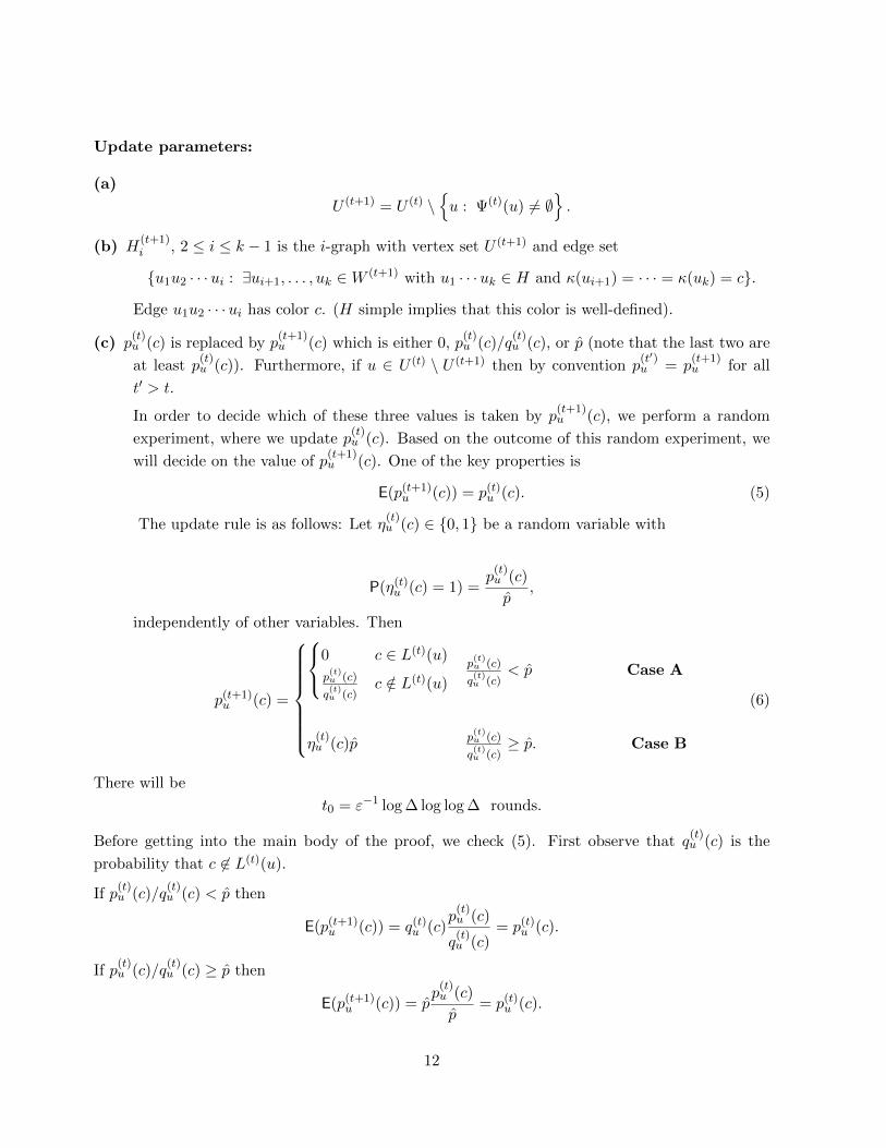
Update parameters:

(a)

U (t+1) = U (t) \u : Ψ(t)(u) 6= ∅

.

(b) H(t+1)i , 2 ≤ i ≤ k − 1 is the i-graph with vertex set U (t+1) and edge set

u1u2 · · ·ui : ∃ui+1, . . . , uk ∈W (t+1) with u1 · · ·uk ∈ H and κ(ui+1) = · · · = κ(uk) = c.

Edge u1u2 · · ·ui has color c. (H simple implies that this color is well-defined).

(c) p(t)u (c) is replaced by p

(t+1)u (c) which is either 0, p

(t)u (c)/q

(t)u (c), or p (note that the last two are

at least p(t)u (c)). Furthermore, if u ∈ U (t) \ U (t+1) then by convention p

(t′)u = p

(t+1)u for all

t′ > t.

In order to decide which of these three values is taken by p(t+1)u (c), we perform a random

experiment, where we update p(t)u (c). Based on the outcome of this random experiment, we

will decide on the value of p(t+1)u (c). One of the key properties is

E(p(t+1)u (c)) = p(t)

u (c). (5)

The update rule is as follows: Let η(t)u (c) ∈ 0, 1 be a random variable with

P(η(t)u (c) = 1) =

p(t)u (c)

p,

independently of other variables. Then

p(t+1)u (c) =

0 c ∈ L(t)(u)

p(t)u (c)

q(t)u (c)

c /∈ L(t)(u)

p(t)u (c)

q(t)u (c)

< p Case A

η(t)u (c)p p

(t)u (c)

q(t)u (c)

≥ p. Case B

(6)

There will be

t0 = ε−1 log ∆ log log ∆ rounds.

Before getting into the main body of the proof, we check (5). First observe that q(t)u (c) is the

probability that c 6∈ L(t)(u).

If p(t)u (c)/q

(t)u (c) < p then

E(p(t+1)u (c)) = q(t)

u (c)p

(t)u (c)

q(t)u (c)

= p(t)u (c).

If p(t)u (c)/q

(t)u (c) ≥ p then

E(p(t+1)u (c)) = p

p(t)u (c)

p= p(t)

u (c).

12

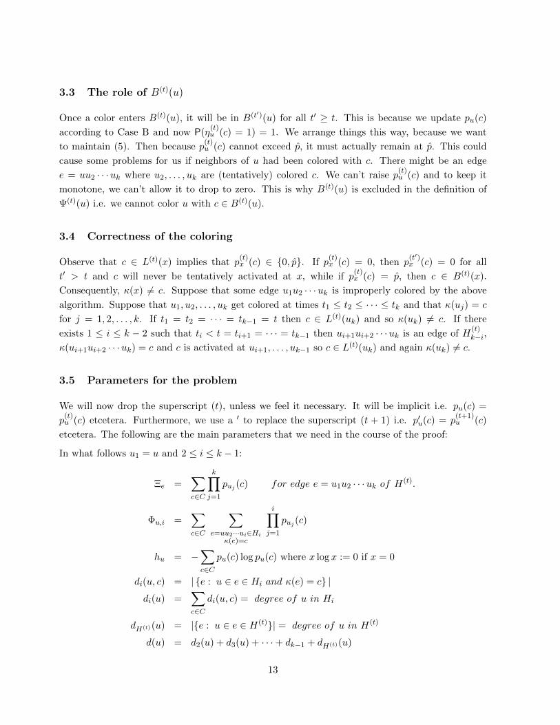
3.3 The role of B(t)(u)

Once a color enters B(t)(u), it will be in B(t′)(u) for all t′ ≥ t. This is because we update pu(c)

according to Case B and now P(η(t)u (c) = 1) = 1. We arrange things this way, because we want

to maintain (5). Then because p(t)u (c) cannot exceed p, it must actually remain at p. This could

cause some problems for us if neighbors of u had been colored with c. There might be an edge

e = uu2 · · ·uk where u2, . . . , uk are (tentatively) colored c. We can’t raise p(t)u (c) and to keep it

monotone, we can’t allow it to drop to zero. This is why B(t)(u) is excluded in the definition of

Ψ(t)(u) i.e. we cannot color u with c ∈ B(t)(u).

3.4 Correctness of the coloring

Observe that c ∈ L(t)(x) implies that p(t)x (c) ∈ 0, p. If p

(t)x (c) = 0, then p

(t′)x (c) = 0 for all

t′ > t and c will never be tentatively activated at x, while if p(t)x (c) = p, then c ∈ B(t)(x).

Consequently, κ(x) 6= c. Suppose that some edge u1u2 · · ·uk is improperly colored by the above

algorithm. Suppose that u1, u2, . . . , uk get colored at times t1 ≤ t2 ≤ · · · ≤ tk and that κ(uj) = c

for j = 1, 2, . . . , k. If t1 = t2 = · · · = tk−1 = t then c ∈ L(t)(uk) and so κ(uk) 6= c. If there

exists 1 ≤ i ≤ k − 2 such that ti < t = ti+1 = · · · = tk−1 then ui+1ui+2 · · ·uk is an edge of H(t)k−i,

κ(ui+1ui+2 · · ·uk) = c and c is activated at ui+1, . . . , uk−1 so c ∈ L(t)(uk) and again κ(uk) 6= c.

3.5 Parameters for the problem

We will now drop the superscript (t), unless we feel it necessary. It will be implicit i.e. pu(c) =

p(t)u (c) etcetera. Furthermore, we use a ′ to replace the superscript (t + 1) i.e. p′u(c) = p

(t+1)u (c)

etcetera. The following are the main parameters that we need in the course of the proof:

In what follows u1 = u and 2 ≤ i ≤ k − 1:

Ξe =∑c∈C

k∏j=1

puj (c) for edge e = u1u2 · · ·uk of H(t).

Φu,i =∑c∈C

∑e=uu2···ui∈Hi

κ(e)=c

i∏j=1

puj (c)

hu = −∑c∈C

pu(c) log pu(c) where x log x := 0 if x = 0

di(u, c) = | e : u ∈ e ∈ Hi and κ(e) = c |di(u) =

∑c∈C

di(u, c) = degree of u in Hi

dH(t)(u) = |e : u ∈ e ∈ H(t)| = degree of u in H(t)

d(u) = d2(u) + d3(u) + · · ·+ dk−1 + dH(t)(u)

13

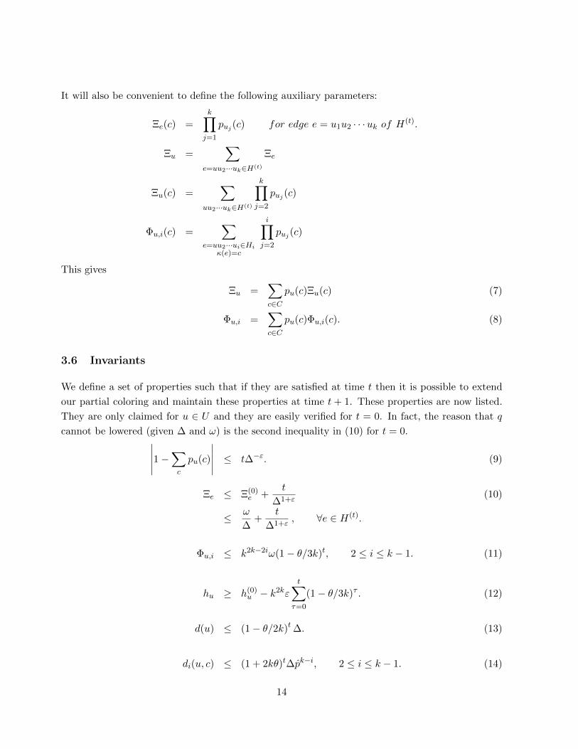
It will also be convenient to define the following auxiliary parameters:

Ξe(c) =k∏j=1

puj (c) for edge e = u1u2 · · ·uk of H(t).

Ξu =∑

e=uu2···uk∈H(t)

Ξe

Ξu(c) =∑

uu2···uk∈H(t)

k∏j=2

puj (c)

Φu,i(c) =∑

e=uu2···ui∈Hiκ(e)=c

i∏j=2

puj (c)

This gives

Ξu =∑c∈C

pu(c)Ξu(c) (7)

Φu,i =∑c∈C

pu(c)Φu,i(c). (8)

3.6 Invariants

We define a set of properties such that if they are satisfied at time t then it is possible to extend

our partial coloring and maintain these properties at time t + 1. These properties are now listed.

They are only claimed for u ∈ U and they are easily verified for t = 0. In fact, the reason that q

cannot be lowered (given ∆ and ω) is the second inequality in (10) for t = 0.∣∣∣∣∣1−∑c

pu(c)

∣∣∣∣∣ ≤ t∆−ε. (9)

Ξe ≤ Ξ(0)e +

t

∆1+ε(10)

≤ ω

∆+

t

∆1+ε, ∀e ∈ H(t).

Φu,i ≤ k2k−2iω(1− θ/3k)t, 2 ≤ i ≤ k − 1. (11)

hu ≥ h(0)u − k2kε

t∑τ=0

(1− θ/3k)τ . (12)

d(u) ≤ (1− θ/2k)t ∆. (13)

di(u, c) ≤ (1 + 2kθ)t∆pk−i, 2 ≤ i ≤ k − 1. (14)

14

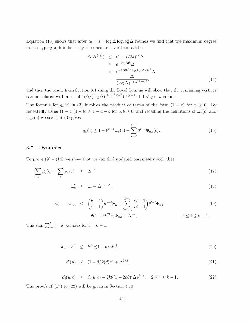
Equation (13) shows that after t0 = ε−1 log ∆ log log ∆ rounds we find that the maximum degree

in the hypergraph induced by the uncolored vertices satisfies

∆(H(t0)) ≤ (1− θ/2k)t0 ∆

≤ e−θt0/2k∆

< e−100k2k log log ∆/2ε2∆

=∆

(log ∆)100k2k/2ε2. (15)

and then the result from Section 3.1 using the Local Lemma will show that the remaining vertices

can be colored with a set of 4(∆/(log ∆)100k2k/2ε2)1/(k−1) + 1 < q new colors.

The formula for qu(c) in (3) involves the product of terms of the form (1 − x) for x ≥ 0. By

repeatedly using (1 − a)(1 − b) ≥ 1 − a − b for a, b ≥ 0, and recalling the definitions of Ξu(c) and

Φu,i(c) we see that (3) gives

qu(c) ≥ 1− θk−1Ξu(c)−k−1∑i=2

θi−1Φu,i(c). (16)

3.7 Dynamics

To prove (9) – (14) we show that we can find updated parameters such that∣∣∣∣∣∑c

p′u(c)−∑c

pu(c)

∣∣∣∣∣ ≤ ∆−ε. (17)

Ξ′e ≤ Ξe + ∆−1−ε. (18)

Φ′u,i − Φu,i ≤(k − 1

i− 1

)θk−iΞu +

k−1∑l=i+1

(l − 1

i− 1

)θl−iΦu,l (19)

−θ(1− 3k2kε)Φu,i + ∆−ε, 2 ≤ i ≤ k − 1.

The sum∑k−1

l=i+1 is vacuous for i = k − 1.

hu − h′u ≤ k2kε(1− θ/3k)t. (20)

d′(u) ≤ (1− θ/k)d(u) + ∆2/3. (21)

d′i(u, c) ≤ di(u, c) + 2kθ(1 + 2kθ)t∆pk−i, 2 ≤ i ≤ k − 1. (22)

The proofs of (17) to (22) will be given in Section 3.10.

15

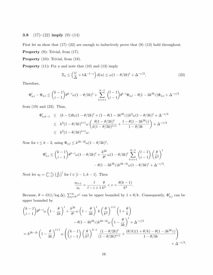
3.8 (17)–(22) imply (9)–(14)

First let us show that (17)–(22) are enough to inductively prove that (9)–(13) hold throughout.

Property (9): Trivial, from (17).

Property (10): Trivial, from (18).

Property (11): Fix u and note that (10) and (13) imply

Ξu ≤( ω

∆+ t∆−1−ε

)d(u) ≤ ω(1− θ/2k)t + ∆−ε/2. (23)

Therefore,

Φ′u,i − Φu,i ≤(k − 1

i− 1

)θk−iω(1− θ/2k)t +

k−1∑l=i+1

(l − 1

i− 1

)θl−iΦu,l − θ(1− 3k2kε)Φu,i + ∆−ε/3

from (19) and (23). Thus,

Φ′u,k−1 ≤ (k − 1)θω(1− θ/2k)t + (1− θ(1− 3k2kε))k2ω(1− θ/3k)t + ∆−ε/3

≤ k2(1− θ/3k)t+1ω

(θ(1− θ/2k)t

k(1− θ/3k)t+1+

1− θ(1− 3k2kε)

1− θ/3k

)+ ∆−ε/3

≤ k2(1− θ/3k)t+1ω.

Now for i ≤ k − 2, using Φu,l ≤ k2k−2lω(1− θ/3k)t,

Φ′u,i ≤(k − 1

i− 1

)θk−iω(1− θ/2k)t +

k2k

θiω(1− θ/3k)t

k−1∑l=i+1

(l − 1

i− 1

)(θ

k2

)l− θ(1− 3k2kε)k2k−2iω(1− θ/3k)t + ∆−ε/3.

Next let ul =(l−1i−1

) (θk2

)lfor l ∈ [i− 1, k − 1]. Then

ul+1

ul=

l

l − i+ 1

θ

k2< r =

θ(k − 1)

k2.

Because, θ = O(1/ log ∆),∑∞

j=0 rj can be upper bounded by 1 + θ/k. Consequently, Φ′u,i can be

upper bounded by(k − 1

i− 1

)θk−iω

(1− θ

2k

)t+k2k

θiω

(1− θ

3k

)tk

(θ

k2

)i+1(1 +

θ

k

)− θ(1− 3k2kε)k2k−2iω

(1− θ

3k

)t+ ∆−ε/3

= k2k−2i

(1− θ

3k

)t+1

ω

((k − 1

i− 1

)(θ

k2

)k−i (1− θ/2k)t

(1− θ/3k)t+1+

(θ/k)(1 + θ/k)− θ(1− 3k2kε)

1− θ/3k

)+ ∆−ε/3.

16

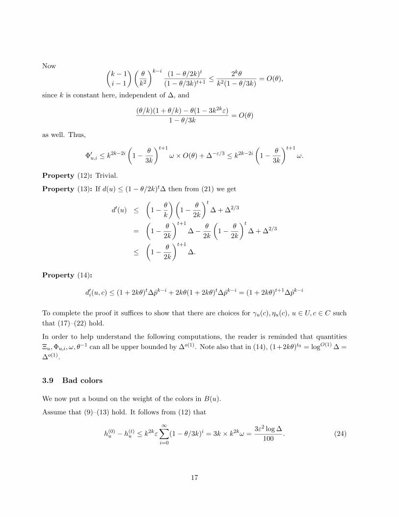
Now (k − 1

i− 1

)(θ

k2

)k−i (1− θ/2k)t

(1− θ/3k)t+1≤ 2kθ

k2(1− θ/3k)= O(θ),

since k is constant here, independent of ∆, and

(θ/k)(1 + θ/k)− θ(1− 3k2kε)

1− θ/3k= O(θ)

as well. Thus,

Φ′u,i ≤ k2k−2i

(1− θ

3k

)t+1

ω ×O(θ) + ∆−ε/3 ≤ k2k−2i

(1− θ

3k

)t+1

ω.

Property (12): Trivial.

Property (13): If d(u) ≤ (1− θ/2k)t∆ then from (21) we get

d′(u) ≤(

1− θ

k

)(1− θ

2k

)t∆ + ∆2/3

=

(1− θ

2k

)t+1

∆− θ

2k

(1− θ

2k

)t∆ + ∆2/3

≤(

1− θ

2k

)t+1

∆.

Property (14):

d′i(u, c) ≤ (1 + 2kθ)t∆pk−i + 2kθ(1 + 2kθ)t∆pk−i = (1 + 2kθ)t+1∆pk−i

To complete the proof it suffices to show that there are choices for γu(c), ηu(c), u ∈ U, c ∈ C such

that (17)–(22) hold.

In order to help understand the following computations, the reader is reminded that quantities

Ξu,Φu,i, ω, θ−1 can all be upper bounded by ∆o(1). Note also that in (14), (1+2kθ)t0 = logO(1) ∆ =

∆o(1).

3.9 Bad colors

We now put a bound on the weight of the colors in B(u).

Assume that (9)–(13) hold. It follows from (12) that

h(0)u − h(t)

u ≤ k2kε

∞∑i=0

(1− θ/3k)i = 3k × k2kω =3ε2 log ∆

100. (24)

17

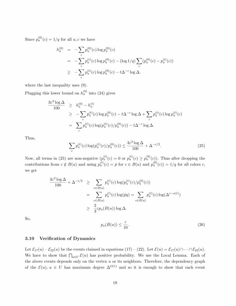
Since p(0)u (c) = 1/q for all u, c we have

h(0)u = −

∑c

p(0)u (c) log p(0)

u (c)

= −∑c

p(t)u (c) log p(0)

u (c)− (log 1/q)∑c

(p(0)u (c)− p(t)

u (c))

≥ −∑c

p(t)u (c) log p(0)

u (c)− t∆−ε log ∆.

where the last inequality uses (9).

Plugging this lower bound on h(0)u into (24) gives

3ε2 log ∆

100≥ h(0)

u − h(t)u

≥ −∑c

p(t)u (c) log p(0)

u (c)− t∆−ε log ∆ +∑c

p(t)u (c) log p(t)

u (c)

=∑c

p(t)u (c) log(p(t)

u (c)/p(0)u (c))− t∆−ε log ∆.

Thus, ∑c

p(t)u (c) log(p(t)

u (c)/p(0)u (c)) ≤ 3ε2 log ∆

100+ ∆−ε/2. (25)

Now, all terms in (25) are non-negative (p(t)u (c) = 0 or p

(t)u (c) ≥ p

(0)u (c)). Thus after dropping the

contributions from c /∈ B(u) and using p(t)u (c) = p for c ∈ B(u) and p

(0)u (c)) = 1/q for all colors c,

we get

3ε2 log ∆

100+ ∆−ε/2 ≥

∑c∈B(u)

p(t)u (c) log(p(t)

u (c)/p(0)u (c))

=∑

c∈B(u)

p(t)u (c) log(pq) =

∑c∈B(u)

p(t)u (c) log(∆ε−o(1))

≥ 2

3εpu(B(u)) log ∆.

So,

pu(B(u)) ≤ ε

10. (26)

3.10 Verification of Dynamics

Let E17(u) – E22(u) be the events claimed in equations (17) – (22). Let E(u) = E17(u)∩· · ·∩E22(u).

We have to show that⋂u∈U E(u) has positive probability. We use the Local Lemma. Each of

the above events depends only on the vertex u or its neighbors. Therefore, the dependency graph

of the E(u), u ∈ U has maximum degree ∆O(1) and so it is enough to show that each event

18

E17(u), . . . , E22(u), u ∈ U has failure probability e−∆Ω(1). For convenience, we will use the notation

whp to stand for with high probability, by which we mean with probability 1− e−∆Ω(1).

While parameters Ξu,Φu etc. are only needed for u ∈ U we do not for example consider Ξ′uconditional on u ∈ U ′. We do not impose this conditioning and so we do not have to deal with it.

Thus the Local Lemma will guarantee a value for Ξu, u ∈ U \U ′ and we are free to disregard it for

the next round. (We will however face this conditioning for other reasons, see (36)).

In the following we will use two forms of Hoeffding’s inequality for sums of bounded random

variables: Suppose first that X1, X2, . . . , Xm are independent random variables and |Xi| ≤ ai for

1 ≤ i ≤ m. Let X = X1 +X2 + · · ·+Xm. Then, for any t > 0,

max P(X − E(X) ≥ t),P(X − E(X) ≤ −t) ≤ exp

− 2t2∑m

i=1 a2i

. (27)

We will also need the following version in the special case that X1, X2, . . . , Xm are independent

[0,1] random variables. For α > 1 we have

P(X ≥ L) ≤ (3/α)L (28)

for any L ≥ αE(X). (We replace e by 3 as the symbol e is over-used in the paper).

For proofs, see for example Alon and Spencer [4], Appendix A and Lugosi [16].

3.10.1 Dependencies

In our random experiment, we start with the pu(c)’s and then we instantiate the independent

random variables γu(c), ηu(c), u ∈ U, c ∈ C and then we compute the p′u(c) from these values.

Observe first that p′u(c) depends only on γv(c), ηv(c) for v = u or v a neighbor of u in H. So p′u(c)

and p′v(c∗) are independent if c 6= c∗, even if u = v. We call this color independence.

Let

Ni(u) = u2, u3, . . . , ui ⊆ U : ∃e ∈ H s.t. u, u2, . . . , ui ⊆ e .

We shorten N2(u) to N(u).

If f = u2, u3, . . . , ui ∈ Ni(u) and l > i, then Eu,f,l = e ∈ Nl(u) : e ⊇ f ∪ u , e ∈ Hl.

Next let

Ni,l(u) = f = u2, . . . , ui ⊆ U : f ∈ Ni(u) and Eu,f,l 6= ∅ , 2 ≤ i < l ≤ k.

In words, Ni,l is the collection of i-sets containing u that are subsets of edges of Hl.

In these definitions Hk = H(t).

For each v ∈ N(u) we let

Cu(v) = c ∈ C : γu(c) = 1 ∪ L(v) ∪B(v).

19

Note that while the first two sets in this union depend on the random choices made in this round,

the set B(v) is already defined at the beginning of the round.

We will later use the fact that if c∗ /∈ Cu(v) and γv(c∗) = 1 then this is enough to place c∗ into

Ψ(v) and allow v to be colored. Indeed, we only need to check that c∗ 6∈ A(t−1)(v) as it will then

follow that c∗ 6∈ A(v). However, γv(c∗) = 1 implies that pv(c

∗) 6= 0 from which it follows that

c∗ 6∈ A(t−1)(v).

Let Yv =∑

c pv(c)1c∈Cu(v) = pv(Cu(v)). Cu(v) is a random set and Yv is the sum of q independent

random variables each one bounded by p. Then by (7), (8) and (16),

E(Yv) ≤∑c∈C

pv(c)P(γu(c) = 1) +∑c∈C

pv(c)(1− qv(c)) + pv(B(v))

≤ θ∑c∈C

pu(c)pv(c) + θk−1Ξv +

k−1∑i=2

θi−1Φv,i + pv(B(v)).

Now let us bound each term separately:

θ∑c∈C

pu(c)pv(c) ≤ θqp2 < θ∆1/(k−1)∆2ε−2/(k−1) <ε

3.

Using (10) we obtain

θk−1Ξv < ωθk−1 + tθk−1∆−ε ≤ εθk−2 + tθk−1∆−ε <ε

6+ε

6=ε

3.

Using (11) we obtain

k−1∑i=2

θi−1Φv,i ≤k−1∑i=2

θi−1k2k−2iω(1− θ/3k)t ≤ k2k−1ε.

Together with P(B(v)) ≤ ε/10 we get

E(Yv) ≤ (k2k−1 + 1)ε.

Hoeffding’s inequality then gives

P(Yv ≥ E(Yv) + ρ) ≤ exp

−2ρ2

qp2

< e−2ρ2∆1/k

.

Taking ρ = ∆−1/2k say, it follows that

P(pv(Cu(v)) ≥ (k2k−1 + 2)ε) = P(Yv ≥ (k2k−1 + 2)ε) ≤ e−∆1/2k. (29)

Let E(29) be the eventpv(Cu(v)) ≤ (k2k−1 + 2)ε

.

Now consider some fixed vertex u ∈ U . It will sometimes be convenient to condition on the values

γx(c), ηx(c) for all c ∈ C and all x /∈ N(u) and for x = u. This conditioning is needed to obtain

independence. We let C denote these conditional values.

20

Remark 8 Note that C determines the set Cu(v), and hence it also determines whether or not

E(29) occurs. Indeed, if γu(c) = 1, then c ∈ Cu(v). On the other hand, if γu(c) = 0 then whether

or not c ∈ L(v) depends only on colors tentatively assigned to vertices not in N(u). This uses the

simplicity and triangle-freeness of H.

Given the conditioning C, simplicity and triangle freeness imply that the events v /∈ U ′, w /∈ U ′for v, w ∈ N(u) are independent provided u, v, w are not part of an edge of H. Indeed, triangle-

freeness implies that in this case, there is no edge containing both v and w. Therefore the random

choices at w will not affect the coloring of v (and vice versa). Thus random variables p′v(c), p′w(c)

will become (conditionally) independent under these circumstances. We call this conditional neigh-

borhood independence.

3.10.1.1 Some expectations

Let us fix a color c and an edge u1u2 · · ·uk ∈ H (here we mean H and not H(t)). In this subsection

we will estimate the expectation of E(∏i

j=1 p′uj (c)

)for 2 ≤ i ≤ k in two distinct situations.

Case 1: i = k and u1u2 · · ·uk ∈ H(t).

Our goal is to prove that

E

k∏j=1

p′uj (c)

≤ (1 + 2kθ2p2)

k∏j=1

puj (c) (30)

If c ∈⋃kj=1A

(t−1)(uj) then∏kj=1 p

′uj (c) = 0. Assume then that c /∈

⋃kj=1A

(t−1)(uj). If Case B of

(6) occurs for any of u1, u2, . . . , uk e.g. uk then

E

k∏j=1

p′uj (c)

∣∣∣∣Case B for k

= E

k−1∏j=1

p′uj (c)

puk(c). (31)

This is because in Case B the value of ηuk(c) is independent of all other random variables and we

may use (5). One can see then that we have to prove something slightly more general than (30).

So we now aim to show that

E

i∏j=1

p′uj (c)

≤ (1 + 2kθ2p2)

i∏j=1

puj (c) (32)

assuming that 1 ≤ i ≤ k and that there is an edge u1u2 · · ·uk ∈ H(t) and that Case A of (6)

happens for uj , c, 1 ≤ j ≤ i. The case i = 1 follows from (5) and so we assume that i ≥ 2. By

simplicity, ui+1, . . . , uk are determined by u1, u2, . . . , ui.

Now∏ij=1 p

′uj (c) = 0 unless c /∈

⋃ij=1 L(uj). Consequently,

E

i∏j=1

p′uj (c)

=i∏

j=1

puj (c)

quj (c)× P

c /∈ i⋃j=1

L(uj)

. (33)

21

Furthermore,

P

c /∈ i⋃j=1

L(uj)

∣∣∣∣γuj (c) = 0, 1 ≤ j ≤ k

=i∏

j=1

quj (c)1− θk−1

∏j′ 6=j

puj′ (c)

−1≤ (1 + 2kθk−1pk−1)

i∏j=1

quj (c)

≤ (1 + 2kθ2p2)i∏

j=1

quj (c).

On the other hand we will show that

P

c /∈ i⋃j=1

L(uj)

∣∣∣∣∃1 ≤ j ≤ k : γuj (c) = 1

≤ P

c /∈ i⋃j=1

L(uj)

∣∣∣∣γuj (c) = 0, 1 ≤ j ≤ k

. (34)

This is intuitively clear, since color c is at least as likely to be lost at uj if it is tentatively activated

at some uj′ . Indeed, to see this formally, partition the probability space Ω of outcomes of the γ’s

and η’s into the sets Ωε1,...,εk in which γuj (c) = εj ∈ 0, 1 for 1 ≤ j ≤ k. Let Ω′ε1,...,εk be the set of

outcomes in Ωε1,...,εk in which c /∈⋃ij=1 L(uj). Now consider the map f : Ωε1,...,εk → Ω′0,...,0 which

just sets γuj (c) to 0 for 1 ≤ j ≤ k. Then if π1j = θpuj (c) and π0

j = 1− π1j

P(Ωε1,...,εk)

P(Ω0,...,0)=

∏kj=1 π

εjj∏k

j=1 π0j

=P(Ω′ε1,...,εk)

P(f(Ω′ε1,...,εk)).

If c 6∈⋃ij=1 L(uj) and ∃1 ≤ j ≤ k such that γuj (c) = 1, then we still have c 6∈

⋃ij=1 L(uj) if we

change γuj (c) to 0 for 1 ≤ j ≤ k and make no other changes. Consequently, f(Ω′ε1,...,εk) ⊆ Ω′0,...,0and we have

P(Ω′0,...,0)

P(Ω0,...,0)≥

P(f(Ω′ε1,...,εk))

P(Ωε1,...,εk)· P(Ωε1,...,εk)

P(Ω0,...,0)=

P(Ω′ε1,...,εk)

P(Ωε1,...,εk),

which is (34).

It follows that

P

c /∈ i⋃j=1

L(uj)

≤ (1 + 2kθ2p2)

i∏j=1

quj (c). (35)

and in combination with (33) this proves (32) and hence (30).

Case 2: e = u1u2 · · ·ui ∈ Hi, κ(e) = c.

Our goal is now to prove

E

i∏j=1

p′uj (c)× 1u2∈U ′

≤ (1− θ(1− 2k2kε))i∏

j=1

puj (c). (36)

22

Suppose that p′uj (c) is determined by Case A of (6) for 1 ≤ j ≤ l and by Case B otherwise.

We factor out∏ij=l+1 puj (c) as in (31). We let L = c /∈ L(u1) ∪ · · ·L(ul) and concentrate on

bounding

E

l∏j=1

p′uj (c)× 1u2∈U ′

=l∏

j=1

puj (c)

quj (c)× P(L ∧ (u2 ∈ U ′))

≤l∏

j=1

puj (c)

quj (c)× P(L)× P(u2 ∈ U ′ | L)

≤l∏

j=1

puj (c)

quj (c)× P(L | γu1(c) = · · · = γul(c) = 0)× P(u2 ∈ U ′ | L) (37)

≤l∏

j=1

puj (c)× (1− θp)−l × P(u2 ∈ U ′ | L). (38)

≤ (1 + kθp)

l∏j=1

puj (c)× P(u2 ∈ U ′ | L).

Explanations: Equation (37) follows as for (34). Equation (38) now follows because the events

c /∈ L(uj) become conditionally independent. And then P(c /∈ L(uj) | γuj (c) = 0) gains a factor(1− θi−1

∏j′ 6=j puj (c)

)−1≤ (1− θp)−1.

Equation (36) will follow once we prove

P(u2 ∈ U ′ | L) ≤ 1− θ(1− k2kε). (39)

Proof of (39):

P(u2 ∈ U ′ | L) = P(u2 ∈ U ′ ∧ γu2(c) = 1 | L) + P(u2 ∈ U ′ ∧ γu2(c) = 0 | L)

≤ P(γu2(c) = 1 | L) +P(u2 ∈ U ′ ∧ L | γu2(c) = 0)P(γu2(c) = 0)

P(L)(40)

≤ P(γu2(c) = 1) +P(u2 ∈ U ′ | γu2(c) = 0)P(L | γu2(c) = 0)P(γu2(c) = 0)

P(L)(41)

≤ P(γu2(c) = 1) + P(u2 ∈ U ′ | γu2(c) = 0)

≤ P(γu2(c) = 1) +P(u2 ∈ U ′)

P(γu2(c) = 0)

≤ θp+P(u2 ∈ U ′)

1− θp. (42)

Explanation: To go from (40) to 41 we have used the following:

(i) P(γu2(c) = 1 | L) ≤ P(γu2(c) = 1), which follows from the FKG inequality. L is monotone

decreasing in the γ’s.

23

(ii) If γu2(c) = 0 then u2 ∈ U ′ is independent of L.

The vertex u2 is colored (i.e., not in U ′) if and only if for some color d /∈ B(u2), γu2(d) = 1 and

d /∈ L(u2). Let Rd denote the event that γu2(d) = 1 and d /∈ L(u2).

P(u2 /∈ U ′) = P

⋃d/∈B(u2)

Rd

≥

∑d/∈B(u2)

P(Rd)−∑

d,d′ /∈B(u2)

P(Rd)P(Rd′)

=∑

d/∈B(u2)

θpu2(d)qu2(d)−∑

d,d′ /∈B(u2)

θ2pu2(d)pu2(d′)qu2(d)qu2(d′)

≥ θ∑d∈C

pu2(d)qu2(d)− θ∑

d∈B(u2)

pu2(d)qu2(d)− θ2∑

d,d′ /∈B(u2)

pu2(d)pu2(d′)

≥ θ∑d∈C

pu2(d)

(1− θk−1Ξu2(d)−

k−1∑i=2

θi−1Φu,i(d)

)− θpu2(B(u2))− θ2

∑d/∈B(u2)

pu2(d)

2

.

after using (16)

≥ θ − θkΞu2 −k−1∑i=2

θiΦu2,i −θε

10− 2θ2

after using (9) and (26)

≥ θ − θk(ω + ∆−ε/2)−k−1∑i=2

θik2k−2iω − θε

10− 2θ2

after using (11) and (23).

Going back to (42) we see that this implies

P(u2 /∈ U ′ | L) ≤ θp+

(1− θ + θk(ω + ∆−ε/2) +

k−1∑i=2

θik2k−2iω +θε

10+ 2θ2

)(1 + 2p)

≤ θp+

(1− θ + 2θk−1ε+ k2k−3θε+

θε

10+ 2θ2

)(1 + 2p)

≤ 1− θ(1− k2kε)

which is (39).

3.10.2 Proof of (17)

Given the pu(c) we see that if Z ′ =∑

c∈C p′u(c) then E(Z ′) =

∑c∈C pu(c). This follows on using

(5). By color independence Z ′ is the sum of q independent non-negative random variables each

24

bounded by p. Applying (27) we see that

P(|Z ′ − E(Z ′)| ≥ ρ) ≤ 2 exp

−2ρ2

qp2

= 2e−2ρ2∆1/(k−1)−2ε−o(1)

.

We take ρ = ∆−ε to see that E17(u) holds whp.

3.10.3 Proof of (18)

Given the pu(c) we see that by (30), Ξ′e has expectation no more than Ξe(1 + 2kθ2p2) and is the

sum of q independent non-negative random variables, each of which is bounded by pk. We have

used color independence again here. Applying (27) we see that

P(Ξ′e ≥ Ξe(1 + 2kθ2pk) + ρ/2) ≤ exp

− ρ2

2qp2k

≤ e−ρ2∆(2k−1)/(k−1)−2kε−o(1)

.

We also have

kΞeθ2p2 ≤ k

(ω

∆+

t

∆1+ε

)θ2p2 <

1

2∆1+ε.

We take ρ = ∆−1−ε to obtain

P(Ξ′e ≥ Ξe + ∆−1−ε) ≤ e−∆Ω(1)

and so E18(u) holds whp.

3.10.4 Proof of (19)

Throughout this section u1 = u. Recall that

Φ′u,i =∑c∈C

∑e=uu2···ui∈H′i

1κ′(e)=c

i∏j=1

p′uj (c).

If e ∈ Hi and κ(e) = c then e ∈ H ′i is equivalent to κ′(e) = c. If κ(e) 6= c but κ′(e) = c then the

edge of H containing u, u2, . . . , ui has some other vertices in U that will be colored with c in the

current round. Consequently, the above expression is

D1 +

k∑l=i+1

D2,l

25

where

D1 =∑c∈C

∑e=uu2···ui∈Hi

κ(e)=c

1κ′(e)=c

i∏j=1

p′uj (c)

D2,k =∑c∈C

∑u2,...ui∈Ni,k(u)

1κ′(uu2···ui)=c

i∏j=1

p′uj (c)

D2,l =∑c∈C

∑u2,...ui∈Ni,l(u)κ(uu2···ul)=c

1κ′(uu2···ui)=c

i∏j=1

p′uj (c) i+ 1 ≤ l ≤ k − 1.

We bound E(D1) and E(D2,i+1), . . . ,E(D2,k) separately.

E(D1):

We write

D1 ≤ D1 =∑c∈C

∑e=uu2···ui∈Hi

κ(e)=c

i∏j=1

p′uj (c)× 1u2∈U ′ .

and then we can use (36) to show

E(D1) ≤ (1− θ(1− 2k2kε))Φu,i. (43)

E(D2,k):

Recall that

D2,k =∑c∈C

∑u2,...,ui∈Ni,k(u)

1κ′(uu2···ui)=c

i∏j=1

p′uj (c).

Instead of summing over sets in Ni,k(u), we may sum over edges uu2 · · ·uk ∈ H(t), and then over

subsets of these edges that lie in Ni,k(u). Thus

D2,k =∑c∈C

∑uu2···uk∈H(t)

∑f⊂u2,...,uk,|f |=i−1

1κ′(f∪u)=c∏

uj∈f∪u1

p′uj (c).

Fix an edge uu2 · · ·uk ∈ H(t). If ui+1, . . . , uk are colored with c in this round, then certainly c

26

must have been tentatively activated at these vertices. Therefore,

E

1κ′(uu2···ui)=c

i∏j=1

p′uj (c)

≤ E

k∏j=i+1

γuj (c)i∏

j=1

p′uj (c)

≤ θk−i

k∏j=i+1

puj (c)

i∏j=1

puj (c)

quj (c)P

c /∈ i⋃j=1

L(uj)

∣∣∣∣ k∧j=i+1

(γuj (c) = 1)

≤ θk−i

k∏j=i+1

puj (c)

i∏j=1

puj (c)

quj (c)P

c /∈ i⋃j=1

L(uj)

(44)

≤ θk−ik∏j=1

puj (c)(1 + 2kθ2p2). (45)

We use the argument for (34) to obtain (44) and (35) to obtain (45).

It follows that

E(D2,k) ≤(k − 1

i− 1

)θk−iΞu(1 + 2kθ2p2). (46)

E(D2,l), i < l < k:

Recall that

D2,l =∑c∈C

∑u2,u3,...ui∈Ni,l(u)

κ(uu2···ul)=c

1κ′(uu2···ui)=c

i∏j=1

p′uj (c).

Fix an edge uu2 · · ·uk ∈ H with uu2 · · ·ul ∈ Hl. Then arguing as we did for (45) we have

E

1κ′(uu2···ui)=c

i∏j=1

p′uj (c)

≤ θl−i l∏j=1

puj (c)(1 + 2kθ2p2).

It follows that

E(D2,l) ≤(l − 1

i− 1

)θl−iΦu,l(1 + 2kθ2p2). (47)

3.10.4.1 Concentration

We first deal with D1. For each color c, let Dc be the event that γv(c) = 1 for at most

d = max di(u, c)p,∆ε vertices v ∈ Ni(u, c) = w : ∃e ∈ Hi such that u, w ∈ e and κ(e) = c.Since P(γv(c) = 1) ≤ pθ,

P(Dc) ≤(

(i− 1)di(u, c)

d

)(θp)d ≤

(ke

p

)d(pθ)d = (keθ)d < e−∆ε

.

Let D denote the event that Dc holds for all c. By the union bound,

P(D) ≤ qe−∆ε.

27

It follows that

E(D1 | D) ≤ (1− qe−∆ε)−1E(D1) ≤ E(D1) + 2q∆e−∆ε

. (48)

Let Tc denote the set of color trials for color c at all vertices in u ∪ N(u) ∪ N(N(u)). Then

the trials T1, . . . , Tq determine the variable D1. Observe that Tc affects every term of the form∏ij=1 p

′uj (c)× 1u2∈U ′ . For d 6= c, Tc affects

∏ij=1 p

′uj (d)× 1u2∈U ′ only if γu2(c) = 1; this is because

if γu2(c) = 0, the trials for color c have no impact on whether or not u2 ∈ U ′. Thus, given D,

changing the values in Tc can change D1 by at most di(u, c)pi + 2di(u, c)p

i+1 + 2∆εpi.

Let π(ti) = P(Ti = ti | D) for i = 1, 2, . . . , q and let

ρ(ti, ti+1, . . . , tq) = π(ti)π(ti+1) · · ·π(tq) = P(Tj = tj , j = i, i+ 1, . . . , q | D).

Here we use the fact that conditioning on D still leaves the choices t1, t2, . . . , tq for the distinct sets

of colors T1, T2, . . . , Tq independent of each other. Thus,

|E[D1|D, T1 = t1, . . . , Tc = tc]− E[D1|D, T1 = t1, . . . , Tc−1 = tc−1, Tc = t′c]| (49)

=

∣∣∣∣∣∣∑

tc+1,...,tq

[D1(t1, . . . , tc−1, tc, tc+1, . . . , tq)− D1(t1, . . . , tc−1, t′c, tc+1, . . . , tq)]ρ(tc+1, . . . , tq)

∣∣∣∣∣∣≤ 3di(u, c)p

i + ∆εpi

≤ 3(1 + 2kθ)t0∆pk + ∆εpi

on using (14)

≤ ∆pk logO(1) ∆ + ∆εpi

≤ ∆(k+1)ε−1/(k−1).

Let δc denote the maximum over t1, t2, . . . , tc, t′c of (49).

P(D1 > (1− θ(1− 2k2kε))Φu,i + ∆−1/2k)

≤ P(D1 > E(D1) + ∆−1/2k)

≤ P(D1 > E(D1 | D) + ∆−1/2k − 2q∆e−∆ε)

≤ P(D1 > E(D1 | D) + ∆−1/2k/2|D) + q∆P(D)

≤ exp

− ∆−1/k

2∑

c δ2c

+ q2∆e−∆ε

(50)

≤ exp

− ∆−1/k

2∆1/(k−1)∆2(k+1)ε−3/(k−1)

+ q2∆e−∆ε

≤ e−∆ε/2. (51)

Equation (50) is a direct application of the Azuma-Hoeffding concentration inequality.

We now deal with the D2,l. There is a minor problem in that the D2,l are sums of random variables

for which we do not have a sufficiently small absolute bound. These variables do however have a

28

small bound which holds with high probability. There are several ways to use this fact. We proceed

as follows: First assume l ≤ k − 1 and let

D2,l,c =∑

u2,u3,...ui∈Ni,l(u)κ(uu2···ul)=c

1κ′(uu2···ui)=c

i∏j=1

p′uj (c)

which we re-write as

D2,l,c =∑

e=uu2···ul∈Hlκ(e)=c

Ze,

where

Zuu2···ul =∑

S⊂u2,u3,...ul|S|=i−1

1κ′(S∪u)=c∏

uj∈S∪u1

p′uj (c).

Then we let

D2,l =∑c∈C

min

(1 + 2kθ)t∆pk, D2,l,c

.

Observe that D2,l is the sum of q independent random variables each bounded by (1 + 2kθ)t∆pk.

So, for ρ > 0,

P(D2,l − E(D2,l) ≥ ρ) ≤ exp

− 2ρ2

∆2+o(1)p2k

≤ e−ρ2∆1/(k−1)−2kε

.

We take ρ = ∆−1/2k to see that

P(D2,l ≥ E(D2,l) + ∆−1/2k) ≤ e−∆ε. (52)

We must of course compare D2,l and D2,l. Now D2,l 6= D2,l only if there exists c such that

D2,l,c > (1 + 2kθ)t∆pk. For each c, D2,l,c is the sum of the dl(u, c) ≤ (1 + 2kθ)t∆pk−l variables

Ze, e ∈ Hl. Each Ze is bounded above by(l−1i−1

)pi and E(Ze) ≤

(l−1i−1

)θl−ipl. This is because Ze is

bounded by the sum of(l−1i−1

)variables Ze,S , each taking the value 0 or pi. Here Ze,S corresponds

to some S = u2, u3, . . . ui ⊆ u2, u3, . . . ul. Furthermore, P(Ze,S = pi) ≤ (θp)l−i because this

will happen only if the vertices in S tentatively choose c.

H being simple and triangle free, if we condition on C then the random variables Ze become

independent.

Now put Xe = Ze/((l−1i−1

)pi) and X =

∑eXe. We see that 0 ≤ Xe ≤ 1 and E(Xe) ≤ (θp)l−i.

We now use (28) with α = 1/((l−1i−1

)θl−i) and E(X) ≤ (1 + 2kθ)t∆pk−l× (θp)l−i = (1+2kθ)t∆pk

α(l−1i−1)pi

. This

gives

P(D2,l,c ≥ (1 + 2kθ)t∆pk | C) ≤ P

(X ≥ (1 + 2kθ)t∆pk(

li

)pi

∣∣∣∣C)≤(

3

(l

i

)θl−i

)(1+2kθ)t∆pk−i/(li)

29

Therefore

P(D2,l 6= D2,l) ≤∑C

P(∃c : D2,l,c ≥ (1 + 2kθ)t∆pk | C)P(C)

≤∑Cq

(3

(l

i

)θl−i

)(1+2kθ)t∆pk−i/(li)P(C)

≤ e−∆ε. (53)

It follows from (53) and D2,l ≤ D2,l ≤ ∆ that

|E(D2,l)− E(D2,l)| ≤ ∆P(D2,l 6= D2,l) ≤ ∆qe−∆ε< ∆−1/2k.

Applying (52) and (53) we see that

P(D2,l ≥ E(D2,l) + 2∆−1/2k) ≤ P(D2,l ≥ E(D2,l) + ∆−1/2k) + P(D2,l 6= D2,l) ≤ 2e−∆ε. (54)

We must now deal with the case of l = k i.e.

D2,k,c =∑

u2,u3,...ui∈Ni,k(u)

1κ′(uu2···ui)=c

i∏j=1

p′uj (c)

and

D2,k =∑c∈C

min

∆pk, D2,k,c

.

We re-write

D2,k,c =∑

S∈Ni,k(u)

WS

where for S = u2, u3, . . . ui,

WS =∑

e⊇S,e∈H(t)

1κ′(uu2···ui)=c

i∏j=1

p′uj (c).

Now we view D2,k,c as the sum of at most ∆ random variables, each of which is bounded by(ki

)pi

and has expectation bounded by(ki

)θk−ipk. We now simply follow the argument for l < k by taking

l = k to show that

P(D2,k ≥ E(D2,k) + 2∆−1/2k) ≤ 2e−∆ε. (55)

Indeed, (52) holds with l = k. Then

P(D2,k 6= D2,k) ≤ qP(Bin

(∆, (θp)k−i

)≥ ∆pk−i

)≤ q

(3θk−i

)∆pk−i

≤ e−∆ε.

30

Combining (54) and (55) with (51) we see that whp,

Φ′u,i − Φu,i ≤ −θ(1− 2k2kε)Φu,i +

(k − 1

i− 1

)θk−iΞu +

k−1∑l=i+1

(l

i− 1

)θl−iΦu,l +

+2k∆−1/2k + 2kθ2p2

((k − 1

i− 1

)θk−iΞu +

k−1∑l=i+1

(l

i− 1

)θl−iΦu,l

)

≤(k − 1

i− 1

)θk−iΞu +

k−1∑l=i+1

(l

i− 1

)θl−iΦu,l − θ(1− 3k2kε)Φu,i + ∆−ε.

This confirms (19).

3.10.5 Proof of (20)

Fix c and write p′ = p′u(c) = pβ. We consider two cases, but in both cases E(β) = 1 and β takes

two values, 0 and 1/P(β > 0). Then we have

E(−p′ log p′) = −p log p− p log(1/P(β > 0)).

(i) p = pu(c) and β = γu(c)/qu(c) and γu(c) is a 0, 1 random variable with P(β > 0) = qu(c).

(ii) p = pu(c) = p and β is a 0, 1 random variable with P(β > 0) = pu(c)/p ≥ qu(c).

Thus in both cases

E(−p′ log p′) ≥ −p log p− p log 1/qu(c).

Observe next that 0 ≤ a, b ≤ 1 implies that (1− ab)−1 ≤ (1 − a)−b and − log(1− x) ≤ x + x2 for

0 ≤ x 1. So, from (3),

log 1/qu(c) ≤ −Ξu(c) log(1− θk−1)−k−1∑i=2

Φu,i(c) log(1− θi−1)

≤ (θk−1 + θ2k−2)Ξu(c) +k−1∑i=2

(θi−1 + θ2i−2)Φu,i(c).

31

Now

E(hu − h′u) ≤ −∑c

pu(c) log pu(c)− E

(∑c

−p′u(c) log p′u(c)

)

≤∑c

−pu(c) log pu(c)−

(∑c

−pu(c) log pu(c)− pu(c) log 1/qu(c)

)=

∑c

pu(c) log 1/qu(c)

≤ (θk−1 + θ2k−2)∑c

pu(c)Ξu(c) +∑c

k−1∑i=2

(θi−1 + θ2i−2)pu(c)Φu,i(c)

= (θk−1 + θ2k−2)Ξu +k−1∑i=2

(θi−1 + θ2i−2)Φu,i

≤ (θk−1 + θ2k−2)(ω + t∆−ε)(1− θ/2k)t +k−1∑i=2

(θi−1 + θ2i−2)k2k−2iω(1− θ/3k)t

≤ k2k−3ε(1− θ/3k)t.

Given the pu(c) we see that h′u is the sum of q independent non-negative random variables with

values bounded by −p log p ≤ ∆−1/(k−1)+ε+o(1). Here we have used color independence. So,

P(hu − h′u ≥ k2k−3ε(1− θ/3k)t + ρ) ≤ exp

− 2ρ2

q(p log p)2

= e−2ρ2∆1/k

.

We take ρ = ε(1− θ/3k)t ≥ (log ∆)−O(1) to see that hu − h′u ≤ k2kε(1− θ/3k)t holds whp.

3.10.6 Proof of (21)

Fix u and condition on the values γw(c), ηw(c) for all c ∈ C and all w /∈ N(u) and for w = u. Now

write u ∼ v to mean that u, v lies in an edge of H(t) or some Hi. Then write

Zu = d(u)− d′(u) ≥ 1

k − 1

∑u∼v

Zu,v where Zu,v = 1v/∈U ′ .

Now, for e = uu2 · · ·uk ∈ H(t) let Zu,e =∑k

j=2 Zu,uj and if e = uu2 · · ·ui ∈ Hi let Zu,e =∑ij=2 Zu,uj . Conditional neighborhood independence implies that the collection Zu,e constitute an

independent set of random variables. Applying (27) to Zu =∑

e Zu,e we see that

P(Zu ≤ E(Zu)−∆2/3) ≤ exp

− 2∆4/3

(k − 1)2∆

= e−2∆1/3/(k−1)2

. (56)

and so we only have to estimate E(Zu).

32

Fix v ∼ u. Let Cu(v) be as in (29). Condition on C. The vertex v is a member of U ′ if none of the

colors c /∈ Cu(v)) are tentatively activated. The activations we consider are done independently

and so

P(v ∈ U ′ | C) ≤∏

c/∈Cu(v)

(1− θpv(c)) (57)

≤ exp

− ∑c/∈Cu(v)

θpv(c)

≤ exp

−θ(1− t∆−ε) + θpv(Cu(v))

If E(29) occurs then pv(Cu(v)) ≤ k2kε. Consequently,

P(v /∈ U ′) ≥∑

C:E(29) occurs

(1− exp

−θ(1−∆−ε) + k2kεθ

)P(C),

where the sum is well-defined due to Remark 8. Since θ → 0 as ∆→∞, and ε is sufficiently small,

1− exp−θ(1−∆−ε) + k2kεθ

> 1− e−θ(1−2k2kε) > θ(1− 3k2kε) > θ(1− 1/k2).

Recall that (29) shows that

P(E(29) fails) ≤ e−∆1/2k< 1/k2.

Therefore

P(v 6∈ U ′) ≥ θ(1− 1/k2)∑

C:E(29) occurs

P(C) > θ(1− 1/k2)2 > θ(1− 1/k).

This gives

E(Zu) ≥ 1

kθd(u)

and (21).

3.10.7 Proof of (22)

Observe that if e = uu2 · · ·ui ∈ H ′i \Hi and κ′(e) = c then either

(i) there exists 1 ≤ j ≤ k − i− 1 and vertices ui+1, . . . , ui+j and an edge uu2 · · ·ui+j ∈ Hi+j such

that ui+1, . . . , ui+j get colored in Step t with c and so γui+1(c) = · · · = γui+j (c) = 1 or

(ii) there exists uu2 · · ·uk ∈ H(t) such that ui+1, . . . , uk all receive the color c and so γui+1(c) =

· · · = γuk(c) = 1. Hence,

d′i(u)− di(u) ≤k−i∑j=1

Zj

where for j ≤ k − i− 1, Zj ≤ Bin((1 + 2kθ)t∆pk−i−j ,(k−ij

)(θp)j) and Zk−i ≤ Bin(∆,

(ki

)(θp)k−i).

33

If i < k − 1, then the Chernoff bound

Pr(Bin(n, p) ≥ 2np) ≤ e−np/3

implies that for 1 ≤ j < k − i,

P

(Zj ≥ 2(1 + 2kθ)t

(k − ij

)θj∆pk−i

)≤ e−∆ε

.

Similarly,

P(Zk−i ≥ 2(1 + 2kθ)tθk−i∆pk−i) ≤ e−∆ε.

Therefore whp

d′i(u, c)− di(u, c) ≤ 2(1 + 2kθ)t∆pk−ik−i∑j=1

(k − ij

)θj

= 2(1 + 2kθ)t∆pk−i((1 + θ)k−i − 1) ≤ 2kθ(1 + 2kθ)t∆pk−i.

4 Acknowledgments

We thank Jeff Cooper for pointing out an error in an earlier draft of this paper and for helpful

subsequent discussions on correcting it. Many thanks also to the referees for their careful reading

and detailed comments which improved the presentation.

References

[1] M. Ajtai, P. Erdos, J. Komlos, E. Szemeredi, On Turan’s theorem for sparse graphs, Combi-

natorica, 1, 313-317 (1981).

[2] M. Ajtai, J. Komlos, J. Pintz, J. Spencer and E. Szemeredi, Extremal uncrowded hypergraphs,

Journal of Combinatorial Theory A 32 (1982), no. 3, 321–335.

[3] N. Alon, M. Krivelevich and B. Sudakov, Coloring graphs with sparse neighborhoods, Journal

of Combinatorial Theory B 77 (1999), 73-82.

[4] N. Alon and J. Spencer, The probabilistic method, Second Edition, Wiley-Interscience, New

Yotk, 2000.

[5] T. Bohman, A. Frieze, D. Mubayi, Coloring H-free hypergraphs, Random Structures and

Algorithms 36 (2010) 11-25.

[6] R. Duke, H. Lefmann, V. Rodl, On uncrowded hypergraphs, Random Structures and Algo-

rithms, 6, 209–212, 1995.

34

[7] P. Erdos, L. Lovasz, Problems and results on 3-chromatic hypergraphs and some related

questions, In Infinite and Finite Sets, A. Hajnal et al., editors, Colloq. Math. Soc. J. Bolyai

11, North Holland, Amsterdam, 609–627, 1975.

[8] A. Frieze and D. Mubayi, On the chromatic number of simple triangle-free triple systems,

Electronic Journal of Combinatorics 15 (2008), no. 1, Research Paper 121, 27 pp.

[9] A. Johansson, Asymptotic choice number for triangle free graphs, DIMACS Technical Report

91-4, 1196.

[10] J. Kahn, Asymptotically good list-colorings, Journal of Combinatorial Theory A 73 (1996),

no. 1, 1–59.

[11] J. H. Kim, On Brooks’ theorem for sparse graphs, Combinatorics, Probability and Computing

4 (1995), no. 2, 97–132.

[12] J. H. Kim and V. Vu, Concentration of multivariate polynomials and its applications, Combi-

natorica 20 (2000) 417-434.

[13] J. Komlos, J. Pintz and E. Szemeredi, A lower bound for Heilbronn’s problem, J. London

Math. Soc. (2) 25 (1982), no. 1, 13–24.

[14] A. Kostochka, D. Mubayi, V. Rodl and P. Tetali, On the chromatic number of set systems,

Random Structures and Algorithms 19 (2001), no. 2, 87–98.

[15] H. Lefmann, Sparse parity-check matrices over GF(q). Combin. Probab. Comput. 14 (2005),

no. 1-2, 147–169.

[16] G. Lugosi, Concentration of measure inequalities, lecture notes for a course given at the Centre

de Recherches Mathematiques, Universite de Montreal, 2005.

[17] V. Rodl, On a packing and covering problem, European Journal of Combinatorics 6 (1985),

no. 1, 69–78.

35