Chi-Square - Wofford Collegewebs.wofford.edu/boppkl/courseFiles/Expmtl/PPTslides/Ch 7_Chi... ·...
32
Chi-Square P216; 269
Transcript of Chi-Square - Wofford Collegewebs.wofford.edu/boppkl/courseFiles/Expmtl/PPTslides/Ch 7_Chi... ·...

Chi-Square
P216; 269

Confidence intervals
CI: % confident that interval contains population mean (µ)
% is determined by researcher (e.g. 85, 90, 95%)
Formula for z-test and t-test: CI = M +/- z*(σM)
CI = M +/- t*(sM)
Where z* or t* is the critical value
Example: CI = 86 +/- 1.96(1.7) = 82.67 to 89.33
95% confident pop mean in this range

Inference by eye: Interpreting CI’s
Why use CI instead of null hypothesis?
Move beyond dichotomous decision
Write-up suggestions “We are 90% confident that the true improvement on the test ranges from 19.75 to 30.25. Values outside of this range are relatively implausible.” “The lower limit of 19.75 is a likely lower bound estimate of improvement.”
Rules of eye What do bars on a graph represent (i.e. sd, se, CI)? Focus on the means, but take variability into account Interpret CI – any value outside CI is “unlikely” Double SE bars to get approximate 95% CI
Chi-square
Method of cooking potato chips
7 16.0 -9.0
33 16.0 17.0
8 16.0 -8.0
48
Fried in animal f at
Fried in Canola oil
Baked
Total
Observ ed N Expected N Residual
Test Statistics
27.125 27.125
2 2
.000 .000
Chi-Squarea
df
Asy mptotic Signif icance
Method of
cooking
potato chips
Number who
pref erred
each type of
chip
0 Cells .0% low f reqs 16.0 expected low...a.
Kristen is interested in evaluating whether the method of cooking potato chips affects the taste of the chips. She tests 48 individuals. Each tastes 3 types of chips, then select which chip they prefer to eat.

Nonparametric tests
Parametric tests: assumptions about population distribution
t-test, ANOVA
Compare means & standard deviations
Nonparametric tests
Chi-square
Compare frequency counts
Evaluate hypotheses about population frequencies
No assumptions regarding population distribution (M, s)

Chi-Square (X2)
Goodness of fit test Uses proportions from sample to examine hypothesis about population proportions
One sample, one variable (but, as many levels as needed)
Test of independence Examines if there is a relationship between two variables
One sample, two variables
Similar to correlation with discrete variables

Chi-square (X2)
Frequency table of data Observed frequencies (fo)
Compare to null hypothesis Expected frequencies (fe)
Null hypothesis No preference No difference vs. comparison population
Expected frequency fe = pn
Chi-square equation df = C – 1, where C = # of categories Chi-square distribution: Table A.4 p410
e
eo
f
ffx
2
2 )(

Chi-square test
Compare observed (O) and expected counts (E)
Measure distance
If distance = 0
then no difference between O & E
= null hypothesis
If distance > 0
then difference between O & E
= evidence against null hypothesis
Chi-square distributions
df based on #cells not n

Goodness of fit: 1 sample
Art appreciation: Painting shown to 50 participants. Asked to hang picture in “correct” orientation.
4 possible ways can hang painting
H0: no preference (25% chance/orientation)
Expected frequencies: .25(50) = 12.5
Top up (correct) Bottom up Left up Right up
12.5 12.5 12.5 12.5
Observed frequencies
Top up (correct) Bottom up Left up Right up
18 17 7 8

Chi-square
table
What is critical value? X2
cv
α = .05
df = 4–1 = 3
7.815

Calculate Chi-square
e
eo
f
ffX
2
2 )(
08.85.12
)5.128(
5.12
)5.127(
5.12
)5.1217(
5.12
)5.1218( 22222
X
Exceeds critical value (7.815), so reject Ho
Observed Frequencies
Expected Frequencies

Chi-square write-up
A chi-square statistic was calculated to examine if there is a preference among four orientations to hang an abstract painting. The test was found to be statistically significant, X2(3, n = 50) = 8.08, p<.05.
The results suggest that participants did not just randomly hang the art on any orientation. Instead it appears the “correct” top-up orientation (p = 18/50) and bottom-up orientation (p = 17/50) were used more often than the left side-up (p = 7/50) or right side-up (p = 8/50) orientation.

Goodness of fit: Chi-square
Assess whether women become less depressed, remain unchanged, or become more depressed after giving birth
Tested 60 women pre and post-birth
Null hypothesis: no difference
Postpartum Depression
14 20.0 -6.0
33 20.0 13.0
13 20.0 -7.0
60
less depressed
same
more depressed
Total
Observ ed N Expected N Residual

SPSS: Chi-square
Postpartum Depression
more depressedsameless depressed
Und
efi
ne
d e
rro
r #
60
86
8 -
Can
no
t o
pe
n t
ex
t fi
le "
sps
s.e
rr":
No s
uch
file
40
30
20
10

SPSS: Chi-square
Postpartum Depression
14 20.0 -6.0
33 20.0 13.0
13 20.0 -7.0
60
less depressed
same
more depressed
Total
Observ ed N Expected N Residual
Test Statistics
12.700
2
.002
Chi-Squarea
df
Asy mptotic Signif icance
Postpartum
Depress ion
0 Cells .0% low f reqs 20.0 expected low.. .a.
Postpartum Depression
14 13.5 .5
13 13.5 -.5
27
less depressed
more depressed
Total
Observ ed N Expected N Residual
Test Statistics
.037
1
.847
Chi-Squarea
df
Asy mptotic Signif icance
Postpartum
Depress ion
0 Cells .0% low f reqs 13.5 expected low.. .a.

Write-up
A one-sample chi-square test was conducted to assess whether women become less depressed, remain unchanged, or become more depressed after giving birth. The results were found to be significant, X2(2, n = 60) = 12.70, p < .01. The proportion of women who were unchanged (55%) was greater than the hypothesized proportion (33%). While women who became less depressed (23%) and more depressed (22%) were approximately the same to the hypothesized proportion. A follow-up test indicated that the proportion of women who became less depressed did not significantly differ from women who became more depressed, X2(1, n = 27) = 0.04, p = ns. Overall, these results suggest that women in general do not become more or less depressed after childbirth.

Goodness of fit hypotheses
Compare proportions of cases with hypothesized values
“Are there more smokers in study than non-smokers?”
No difference in categories H0: 50% smokers; 50% non-smokers
Or specific proportions obtained from prior studies
H0: 20% smokers; 80% non-smokers

Write-up
A chi-square goodness of fit test indicates there was no significant difference in the proportion of smokers identified in the current sample (19.5%) as compared with the value in the nationwide study (20%), X2 (1, n = 436) = .07, p = .79.
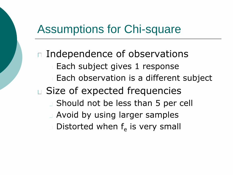
Assumptions for Chi-square
Independence of observations
Each subject gives 1 response
Each observation is a different subject
Size of expected frequencies
Should not be less than 5 per cell
Avoid by using larger samples
Distorted when fe is very small

Chi-square (X2)
Goodness of fit test
Null hypothesis
No preference hypothesis
Test for independence – 2 variables!
Null hypothesis
Same proportions for 2 variables
i.e. no relationship between variables

Treating Cocaine Addiction
0
2
4
6
8
10
12
14
16
18
20
Desipramine Lithium Placebo
Success
Relapse

Independence Chi-square test: 2 variables
Examine relationship between 2 variables
Treating cocaine addiction
No Yes
Desipramine 14 10
Lithium 6 18
Placebo 4 20
Relapse
Total
24
24
24
72Total 24 48
Compare study findings to expected findings
n
fff rce
No relapse: 24*24/72 = 8 (successes expected/drug)
Yes relapse: 48*24/72 = 16 (failures expected/drug)

Independence Chi-square test
Null hypothesis: no relationship between type of drug and relapse
df = (R – 1)(C – 1) = 2-1(3-1) = 2
Critical value X2 @ .05 = 5.99
Significant!
Examine proportions (#/total) of no relapse
Drug1: 14/24 = .58, Drug2: 6/24 = .25, Drug3: 4/24 = .17 (vs. expected: 8/24 = .33)
e
eo
f
ffX
2
2 )(
5.1016
)1620(
16
)1618(
16
)1610(
8
)84(
8
)86(
8
)814( 2222222
X
No Yes
Desipramine 14 / 8 10 / 16
Lithium 6 / 8 18 / 16
Placebo 4 / 8 20 / 16
Relapse

Write-up
A chi-square test was conducted to assess whether cocaine addicts would relapse when treating addiction with Desipramine, Lithium, or a placebo drug. The results were found to be significant, X2(2, n = 72) = 10.5, p < .05.
The proportion of addicts who did not relapse when treated with Desipramine (58%) was greater than the hypothesized proportion (33%). While the number of addicts who did not relapse when treated with Lithium (25%) and the placebo (17%) were approximately the same than the hypothesized proportion.
The results suggest that there is a relationship between probability of a relapse and drug used to treat the addiction. It appears that Desipramine assists cocaine addicts to prevent relapse of drug abuse.

Gender and smoking example
Is there an association between gender and smoking behavior? Is the proportion of males that smoke the same as the proportion of females?
Write-up
A chi-square test for independence indicated no significant difference in the proportion of males or females that smoke, X2(1, n = 436) = 0.494, p = .48.

Other non-parametric statistics
Mann-Whitney U test Equivalent to independent-samples t-test
DV (scores) converted to ranks; examine median
Ex. IV: gender; DV: self-esteem rank
Wilcoxon signed rank test Equivalent to paired-samples t-test
Converts scores to ranks; compares T1 & T2
Kruskal-Wallis test Equivalent to one-way ANOVA
Scores converted to ranks; 1 bet-Ss IV w/ 3+ levels
Friedman test Equivalent to repeated-measures ANOVA
Scores converted to ranks; 1 w/in Ss IV w/ 3+ levels

Chapter 13
Quasi-experimental research Non-manipulated IV: Ss not randomly assigned to condition
Lacks internal validity (confounding variable?)
Quasi-experimental designs One sample
Single-group posttest only design
Single-group pre/posttest design
Single-group time-series design
Two samples Nonequivalent control group posttest only design
Nonequivalent control group pre/posttest design
Multiple-group time-series design

Chapter 13
Cross-sectional design
Ss at different ages at one testing time
Pro: fast and cheap
Con: possible cohort effect
Longitudinal design
Ss repeatedly tested over time
Pro: examine “change” (age effect)
Con: attrition
Sequential design
Mix of cross-sectional and longitudinal
Pro: benefits of both cross/longitudinal designs
Con: statistics are difficult/unknown

Schaie, K. W. (1994). The course of adult intellectual
development. American Psychologist, 49, 304-313.

Figure 2. Cross-Sectional Mean T Scores for Single Markers of the Primary Mental Abilities
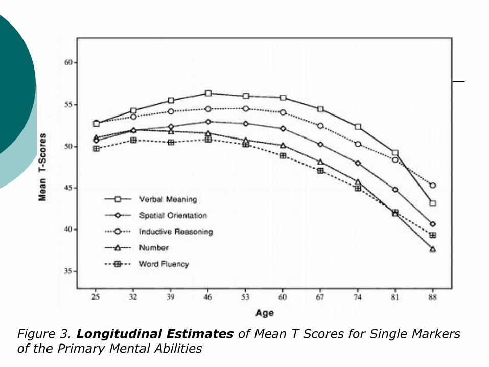
Figure 3. Longitudinal Estimates of Mean T Scores for Single Markers of the Primary Mental Abilities