Efficient Logistic Regression with Stochastic Gradient Descent – part 2
Chapter 5: Logistic Regression-II
Dipankar Bandyopadhyay
Department of Biostatistics,Virginia Commonwealth University
BIOS 625: Categorical Data & GLM
[Acknowledgements to Tim Hanson and Haitao Chu]
D. Bandyopadhyay (VCU) 1 / 37
Chapter 5 5.3 Categorical Predictors: Continued
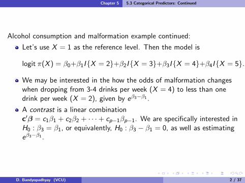
Alcohol consumption and malformation example continued:
Let’s use X = 1 as the reference level. Then the model is
logit π(X ) = β0+β1I{X = 2}+β2I{X = 3}+β3I{X = 4}+β4I{X = 5}.
We may be interested in the how the odds of malformation changeswhen dropping from 3-4 drinks per week (X = 4) to less than onedrink per week (X = 2), given by eβ3−β1 .
A contrast is a linear combinationc′β = c1β1 + c2β2 + · · ·+ cp−1βp−1. We are specifically interested inH0 : β3 = β1, or equivalently, H0 : β3 − β1 = 0, as well as estimatingeβ3−β1 .
D. Bandyopadhyay (VCU) 2 / 37
Chapter 5 5.3 Categorical Predictors: Continued
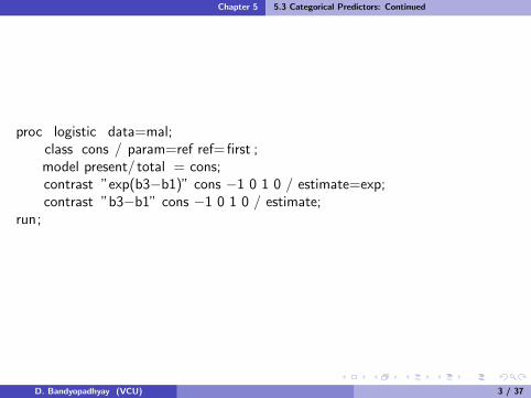
proc logistic data=mal;class cons / param=ref ref= first ;model present/ total = cons;contrast ”exp(b3−b1)” cons −1 0 1 0 / estimate=exp;contrast ”b3−b1” cons −1 0 1 0 / estimate;
run;
D. Bandyopadhyay (VCU) 3 / 37
Chapter 5 5.3 Categorical Predictors: Continued
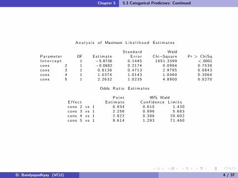
Ana l y s i s o f Maximum L i k e l i h o o d Es t ima t e s
Standard WaldParameter DF Est imate E r r o r Chi−Square Pr > ChiSqI n t e r c e p t 1 −5.8736 0 .1445 1651.3399 <.0001cons 2 1 −0.0682 0 .2174 0 .0984 0 .7538cons 3 1 0 .8136 0 .4713 2 .9795 0 .0843cons 4 1 1 .0374 1 .0143 1 .0460 0 .3064cons 5 1 2 .2632 1 .0235 4 .8900 0 .0270
Odds Rat i o E s t ima t e s
Po in t 95% WaldE f f e c t Es t imate Con f i d ence L im i t scons 2 vs 1 0 .934 0 .610 1 .430cons 3 vs 1 2 .256 0 .896 5 .683cons 4 vs 1 2 .822 0 .386 20 .602cons 5 vs 1 9 .614 1 .293 71 .460
D. Bandyopadhyay (VCU) 4 / 37
Chapter 5 5.3 Categorical Predictors: Continued
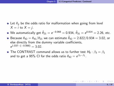
Let θij be the odds ratio for malformation when going from levelX = i to X = j .
We automatically get θ21 = e−0.068 = 0.934, θ31 = e0.814 = 2.26, etc.
Because θ42 = θ41/θ21 we can estimate θ42 = 2.822/0.934 = 3.02, orelse directly from the dummy variable coefficients,e1.037−(−0.068) = 3.02.
The CONTRAST command allows us to further test H0 : β3 = β1and to get a 95% CI for the odds ratio θ42 = eβ3−β1 .
D. Bandyopadhyay (VCU) 5 / 37
Chapter 5 5.3 Categorical Predictors: Continued
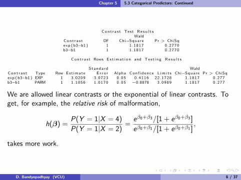
Cont r a s t Test R e s u l t sWald
Con t r a s t DF Chi−Square Pr > ChiSqexp ( b3−b1 ) 1 1 .1817 0 .2770b3−b1 1 1 .1817 0 .2770
Con t r a s t Rows E s t ima t i on and Tes t i ng R e s u l t s
Standard WaldCon t r a s t Type Row Est imate E r r o r Alpha Con f i d ence L im i t s Chi−Square Pr > ChiSqexp ( b3−b1 ) EXP 1 3.0209 3 .0723 0 .05 0 .4116 22.1728 1 .1817 0 .277b3−b1 PARM 1 1.1056 1 .0170 0 .05 −0.8878 3 .0989 1 .1817 0 .277
We are allowed linear contrasts or the exponential of linear contrasts. Toget, for example, the relative risk of malformation,
h(β) =P(Y = 1|X = 4)
P(Y = 1|X = 2)=
eβ0+β3/[1 + eβ0+β3 ]
eβ0+β1/[1 + eβ0+β1 ],
takes more work.
D. Bandyopadhyay (VCU) 6 / 37
Chapter 5 5.3 Categorical Predictors: Continued
5.3.4 I × 2 tables
Let X = 1, 2, . . . , I be an ordinal predictor.
If the log odds increases linearly with category X = i we havelogit π(i) = α + βi .
If the log risk increases linearly we have logπ(i) = α + βi .
If the probability increases linearly we have π(i) = α + βi .
If we replace X = 1, 2, . . . , I by scores u1 ≤ u2 ≤ · · · ≤ uI , we get
logit linear model: logit π(i) = α + βui ,
log linear model: logπ(i) = α + βui ,
linear model: π(i) = α + βui .
D. Bandyopadhyay (VCU) 7 / 37
Chapter 5 5.3 Categorical Predictors: Continued
In any of these models testing H0 : β = 0 is a test of X ⊥ Y versus aparticular monotone alternative.
The last of the six is called the Cochran-Armitage linear trend model.
Tarone and Gart (1980) Showed that the score test(Cochran-Armitage trend test) for a binary linear trend model doesnot depend on the link function.
These can all be fit in SAS GENMOD.
proc genmod; model present/total = cons / dist=bin link=logit ;proc genmod; model present/total = cons / dist=bin link=log;proc genmod; model present/total = cons / dist=bin link=identity ;proc genmod; model present/total = score / dist =bin link=logit ;proc genmod; model present/total = score / dist =bin link=log;proc genmod; model present/total = score / dist =bin link=identity ;
D. Bandyopadhyay (VCU) 8 / 37
Chapter 5 5.3 Categorical Predictors: Continued
The first three use X = 1, 2, 3, 4, 5 and the last three useX = 0.0, 0.5, 1.5, 4.0, 7.0.
For this data, the p-values are respectively 0.18, 0.18, 0.28, 0.01,0.01, 0.13 testing H0 : β1 = 0 using Wald test.
The Pearson GOF X 2 = 2.05 with p = 0.56 for the logit model withscores and X 2 = 5.68 with p = 0.13 for using 1, 2, 3, 4, 5. The logitmodel using scores fits better and from this model we rejectH0 : β = 0 with p = 0.01.
D. Bandyopadhyay (VCU) 9 / 37
Chapter 5 5.4 Multiple Predictors
Now we have p − 1 predictors xi = (1, xi1, . . . , xi ,p−1) and fit
Yi ∼ bin
(ni ,
exp(β0 + β1xi1 + · · ·+ βp−1xi ,p−1)
1 + exp(β0 + β1xi1 + · · ·+ βp−1xi ,p−1)
).
Many of these predictors may be sets of dummy variables associatedwith categorical predictors.
eβj is now termed the adjusted odds ratio. This is how the odds ofthe event occurring changes when xj increases by one unit keepingthe remaining predictors constant.
This interpretation may not make sense if two predictors are highlyrelated.
D. Bandyopadhyay (VCU) 10 / 37
Chapter 5 5.4 Multiple Predictors
An overall test of H0 : logit π(x) = β0 versus H1 : logit π(x) = x′β isgenerated in PROC LOGISTIC three different ways: LRT, score, and Waldversions. This checks whether some subset of variables in the model isimportant.Recall the crab data covariates:
C = color (1,2,3,4=light medium, medium, dark medium, dark).
S = spine condition (1,2,3=both good, one worn or broken, bothworn or borken).
W = carapace width (cm).
Wt = weight (kg).
We’ll take C = 4 and S = 3 as baseline categories.
D. Bandyopadhyay (VCU) 11 / 37
Chapter 5 5.4 Multiple Predictors
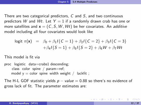
There are two categorical predictors, C and S , and two continuouspredictors W and Wt. Let Y = 1 if a randomly drawn crab has one ormore satellites and x = (C ,S ,W ,Wt) be her covariates. An additivemodel including all four covariates would look like
logit π(x) = β0 + β1I{C = 1}+ β2I{C = 2}+ β3I{C = 3}+β4I{S = 1}+ β5I{S = 2}+ β6W + β7Wt
This model is fit via
proc logistic data=crabs1 descending;class color spine / param=ref;model y = color spine width weight / lackfit ;
The H-L GOF statistic yields p − value = 0.88 so there’s no evidence ofgross lack of fit. The parameter estimates are:
D. Bandyopadhyay (VCU) 12 / 37
Chapter 5 5.4 Multiple Predictors
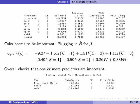
Standard WaldParameter DF Est imate E r r o r Chi−Square Pr > ChiSqI n t e r c e p t 1 −9.2734 3 .8378 5 .8386 0 .0157c o l o r 1 1 1 .6087 0 .9355 2 .9567 0 .0855c o l o r 2 1 1 .5058 0 .5667 7 .0607 0 .0079c o l o r 3 1 1 .1198 0 .5933 3 .5624 0 .0591s p i n e 1 1 −0.4003 0 .5027 0 .6340 0 .4259s p i n e 2 1 −0.4963 0 .6292 0 .6222 0 .4302width 1 0 .2631 0 .1953 1 .8152 0 .1779we ight 1 0 .8258 0 .7038 1 .3765 0 .2407
Color seems to be important. Plugging in β for β,
logit π(x) = −9.27 + 1.61I{C = 1}+ 1.51I{C = 2}+ 1.11I{C = 3}−0.40I{S = 1} − 0.50I{S = 2}+ 0.26W + 0.83Wt
Overall checks that one or more predictors are important:
Tes t i ng G l oba l Nu l l Hypo the s i s : BETA=0
Test Chi−Square DF Pr > ChiSqL i k e l i h o o d Rat i o 40 .5565 7 <.0001Score 36 .3068 7 <.0001Wald 29 .4763 7 0 .0001
D. Bandyopadhyay (VCU) 13 / 37
Chapter 5 5.4 Multiple Predictors
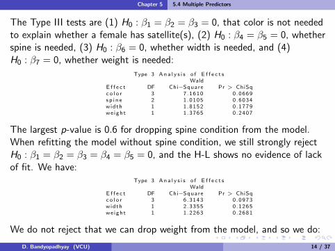
The Type III tests are (1) H0 : β1 = β2 = β3 = 0, that color is not neededto explain whether a female has satellite(s), (2) H0 : β4 = β5 = 0, whetherspine is needed, (3) H0 : β6 = 0, whether width is needed, and (4)H0 : β7 = 0, whether weight is needed:
Type 3 An a l y s i s o f E f f e c t sWald
E f f e c t DF Chi−Square Pr > ChiSqc o l o r 3 7 .1610 0 .0669s p i n e 2 1 .0105 0 .6034width 1 1 .8152 0 .1779we ight 1 1 .3765 0 .2407
The largest p-value is 0.6 for dropping spine condition from the model.When refitting the model without spine condition, we still strongly rejectH0 : β1 = β2 = β3 = β4 = β5 = 0, and the H-L shows no evidence of lackof fit. We have:
Type 3 An a l y s i s o f E f f e c t sWald
E f f e c t DF Chi−Square Pr > ChiSqc o l o r 3 6 .3143 0 .0973width 1 2 .3355 0 .1265we ight 1 1 .2263 0 .2681
We do not reject that we can drop weight from the model, and so we do:
D. Bandyopadhyay (VCU) 14 / 37
Chapter 5 5.4 Multiple Predictors
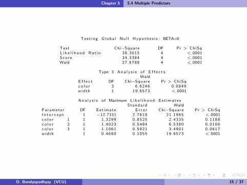
Tes t i ng G l oba l Nu l l Hypo the s i s : BETA=0
Test Chi−Square DF Pr > ChiSqL i k e l i h o o d Rat i o 38 .3015 4 <.0001Score 34 .3384 4 <.0001Wald 27 .6788 4 <.0001
Type 3 An a l y s i s o f E f f e c t sWald
E f f e c t DF Chi−Square Pr > ChiSqc o l o r 3 6 .6246 0 .0849width 1 19.6573 <.0001
An a l y s i s o f Maximum L i k e l i h o o d Es t ima t e sStandard Wald
Parameter DF Est imate E r r o r Chi−Square Pr > ChiSqI n t e r c e p t 1 −12.7151 2 .7618 21.1965 <.0001c o l o r 1 1 1 .3299 0 .8525 2 .4335 0 .1188c o l o r 2 1 1 .4023 0 .5484 6 .5380 0 .0106c o l o r 3 1 1 .1061 0 .5921 3 .4901 0 .0617width 1 0 .4680 0 .1055 19.6573 <.0001
D. Bandyopadhyay (VCU) 15 / 37
Chapter 5 5.4 Multiple Predictors
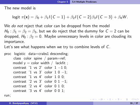
The new model is
logit π(x) = β0 + β1I{C = 1}+ β2I{C = 2}β3I{C = 3}+ β4W .
We do not reject that color can be dropped from the modelH0 : β1 = β2 = β3, but we do reject that the dummy for C = 2 can bedropped, H0 : β2 = 0. Maybe unnecessary levels in color are clouding itsimportance.Let’s see what happens when we try to combine levels of C .
proc logistic data=crabs1 descending;class color spine / param=ref;model y = color width / lackfit ;contrast ’1 vs 2’ color 1 −1 0;contrast ’1 vs 3’ color 1 0 −1;contrast ’1 vs 4’ color 1 0 0;contrast ’2 vs 3’ color 0 1 −1;contrast ’2 vs 4’ color 0 1 0;contrast ’3 vs 4’ color 0 0 1;
run;
D. Bandyopadhyay (VCU) 16 / 37
Chapter 5 5.4 Multiple Predictors
p-values for combining levels:
Cont r a s t Test R e s u l t sWald
Con t r a s t DF Chi−Square Pr > ChiSq1 vs 2 1 0 .0096 0 .92201 vs 3 1 0 .0829 0 .77331 vs 4 1 2 .4335 0 .11882 vs 3 1 0 .5031 0 .47812 vs 4 1 6 .5380 0 .01063 vs 4 1 3 .4901 0 .0617
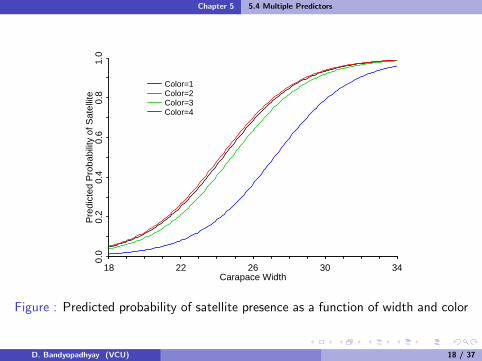
We reject that we can combine levels C = 2 and C = 4, and almostreject combining C = 3 and C = 4. Let’s combine C = 1, 2, 3 intoone category D = 1 “not dark” and C = 4 is D = 2, “dark”. SeeFigure 5.7 (p.188) in next slide.
D. Bandyopadhyay (VCU) 17 / 37
Chapter 5 5.4 Multiple Predictors
Carapace Width
Pre
dict
ed P
roba
bilit
y of
Sat
ellit
e0.
00.
20.
40.
60.
81.
0
18 22 26 30 34
Color=1Color=2Color=3Color=4
Figure : Predicted probability of satellite presence as a function of width and color
D. Bandyopadhyay (VCU) 18 / 37
Chapter 5 5.4 Multiple Predictors
We include dark=1; if color=4 then dark=2; in the DATA step,and fit
proc logistic data=crabs1 descending;class dark / param=ref ref= first ;model y = dark width / lackfit ;run;
Annotated output:
D. Bandyopadhyay (VCU) 19 / 37
Chapter 5 5.4 Multiple Predictors
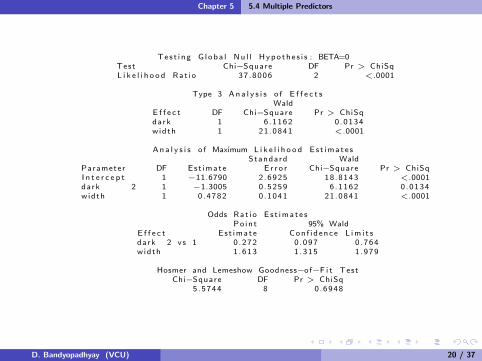
Tes t i ng G l oba l Nu l l Hypo the s i s : BETA=0Test Chi−Square DF Pr > ChiSqL i k e l i h o o d Rat i o 37 .8006 2 <.0001
Type 3 An a l y s i s o f E f f e c t sWald
E f f e c t DF Chi−Square Pr > ChiSqdark 1 6 .1162 0 .0134width 1 21.0841 <.0001
An a l y s i s o f Maximum L i k e l i h o o d Es t ima t e sStandard Wald
Parameter DF Est imate E r r o r Chi−Square Pr > ChiSqI n t e r c e p t 1 −11.6790 2 .6925 18.8143 <.0001dark 2 1 −1.3005 0 .5259 6 .1162 0 .0134width 1 0 .4782 0 .1041 21.0841 <.0001
Odds Rat i o E s t ima t e sPo in t 95% Wald
E f f e c t Es t imate Con f i d ence L im i t sdark 2 vs 1 0 .272 0 .097 0 .764width 1 .613 1 .315 1 .979
Hosmer and Lemeshow Goodness−of−F i t TestChi−Square DF Pr > ChiSq
5 .5744 8 0 .6948
D. Bandyopadhyay (VCU) 20 / 37
Chapter 5 5.4 Multiple Predictors
Comments:
The odds of having satellite(s) significantly decreases by a little lessthan a third, 0.27, for dark crabs regardless of width.
The odds of having satellite(s) significantly increases by a factor of1.6 for every cm increase in carapice width regardless of color.
Lighter, wider crabs tend to have satellite(s) more often.
The H-L GOF test shows no gross LOF.
We didn’t check for interactions. If an interaction between color andwidth existed, then the odds ratio of satellite(s) for dark versus notdark crabs would change with how wide she is.
D. Bandyopadhyay (VCU) 21 / 37
Chapter 5 5.4 Multiple Predictors
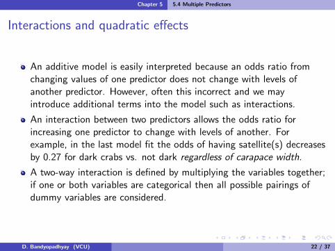
Interactions and quadratic effects
An additive model is easily interpreted because an odds ratio fromchanging values of one predictor does not change with levels ofanother predictor. However, often this incorrect and we mayintroduce additional terms into the model such as interactions.
An interaction between two predictors allows the odds ratio forincreasing one predictor to change with levels of another. Forexample, in the last model fit the odds of having satellite(s) decreasesby 0.27 for dark crabs vs. not dark regardless of carapace width.
A two-way interaction is defined by multiplying the variables together;if one or both variables are categorical then all possible pairings ofdummy variables are considered.
D. Bandyopadhyay (VCU) 22 / 37
Chapter 5 5.4 Multiple Predictors
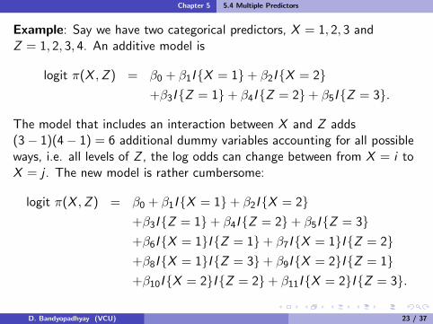
Example: Say we have two categorical predictors, X = 1, 2, 3 andZ = 1, 2, 3, 4. An additive model is
logit π(X ,Z ) = β0 + β1I{X = 1}+ β2I{X = 2}+β3I{Z = 1}+ β4I{Z = 2}+ β5I{Z = 3}.
The model that includes an interaction between X and Z adds(3− 1)(4− 1) = 6 additional dummy variables accounting for all possibleways, i.e. all levels of Z , the log odds can change between from X = i toX = j . The new model is rather cumbersome:
logit π(X ,Z ) = β0 + β1I{X = 1}+ β2I{X = 2}+β3I{Z = 1}+ β4I{Z = 2}+ β5I{Z = 3}+β6I{X = 1}I{Z = 1}+ β7I{X = 1}I{Z = 2}+β8I{X = 1}I{Z = 3}+ β9I{X = 2}I{Z = 1}+β10I{X = 2}I{Z = 2}+ β11I{X = 2}I{Z = 3}.
D. Bandyopadhyay (VCU) 23 / 37

Chapter 5 5.4 Multiple Predictors
In PROC GENMOD and PROC LOGISTIC, categorical variables aredefined through the CLASS statement and all dummy variables arecreated and handled internally.
The Type III table provides a test that the interaction can bedropped; the table of regression coefficients tell you whetherindividual dummies can be dropped.
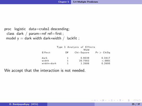
Let’s consider the crab data again, but consider an interactionbetween categorical D and continuous W :
D. Bandyopadhyay (VCU) 24 / 37
Chapter 5 5.4 Multiple Predictors
proc logistic data=crabs1 descending;class dark / param=ref ref= first ;model y = dark width dark∗width / lackfit ;
Type 3 An a l y s i s o f E f f e c t sWald
E f f e c t DF Chi−Square Pr > ChiSq
dark 1 0 .9039 0 .3417width 1 20.7562 <.0001width∗dark 1 1 .2686 0 .2600
We accept that the interaction is not needed.
D. Bandyopadhyay (VCU) 25 / 37
Chapter 5 5.4 Multiple Predictors
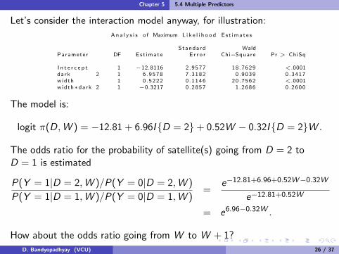
Let’s consider the interaction model anyway, for illustration:
Ana l y s i s o f Maximum L i k e l i h o o d Es t ima t e s
Standard WaldParameter DF Es t imate E r r o r Chi−Square Pr > ChiSq
I n t e r c e p t 1 −12.8116 2 .9577 18.7629 <.0001dark 2 1 6 .9578 7 .3182 0 .9039 0 .3417width 1 0 .5222 0 .1146 20.7562 <.0001width∗dark 2 1 −0.3217 0 .2857 1 .2686 0 .2600
The model is:
logit π(D,W ) = −12.81 + 6.96I{D = 2}+ 0.52W − 0.32I{D = 2}W .
The odds ratio for the probability of satellite(s) going from D = 2 toD = 1 is estimated
P(Y = 1|D = 2,W )/P(Y = 0|D = 2,W )
P(Y = 1|D = 1,W )/P(Y = 0|D = 1,W )=
e−12.81+6.96+0.52W−0.32W
e−12.81+0.52W
= e6.96−0.32W .
How about the odds ratio going from W to W + 1?
D. Bandyopadhyay (VCU) 26 / 37
Chapter 5 5.4 Multiple Predictors
For a categorical predictor X with I levels, adding I − 1 dummyvariables allows for a different event probability at each level of X .
For a continuous predictor Z , the model assumes that the log-odds ofthe event increases linearly with Z . This may or may not be areasonable assumption, but can be checked by adding nonlinearterms, the simplest being Z 2.
Consider a simple model with continuous Z :
logit π(Z ) = β0 + β1Z .
LOF from this model can manifest itself in rejecting a GOF test(Pearson, deviance, or H-L) or a residual plot that shows curvature.
D. Bandyopadhyay (VCU) 27 / 37
Chapter 5 5.4 Multiple Predictors
Adding a quadratic term
logit π(Z ) = β0 + β1Z + β2Z2,
may improve fit and allows testing the adequacy of the simpler model viaH0 : β2 = 0. Higher order powers can be added, but the model canbecome unstable with, say, higher than cubic powers. A better approachmight be to fit a generalized additive model (GAM):
logit π(Z ) = f (Z ),
where f (·) is estimated from the data, often using splines.However, we will not discuss this in this course!Adding a simple quadratic term can be done, e.g.,proc logistic; model y/n = z z*z;
D. Bandyopadhyay (VCU) 28 / 37
Chapter 5 5.4 Multiple Predictors
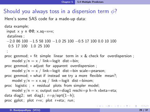
Should you always toss in a dispersion term φ?Here’s some SAS code for a made-up data:
data example;input x y n @@; x sq=x∗x;datalines ;−2.0 86 100 −1.5 58 100 −1.0 25 100 −0.5 17 100 0.0 10 100
0.5 17 100 1.0 25 100;
proc genmod; ∗ fit simple linear term in x & check for overdispersion ;model y/n = x / link=logit dist =bin;
proc genmod; ∗ adjust for apparent overdispersion ;model y/n = x / link=logit dist =bin scale=pearson;
proc genmod; ∗ what if instead we try a more flexible mean?;model y/n = x x sq / link =logit dist =binom;
proc logistic ; ∗ residual plots from simpler model;model y/n = x; output out=diag1 reschi=p h=h xbeta=eta;
data diag2; set diag1; r=p/sqrt(1−h);proc gplot ; plot r∗x; plot r∗eta; run;
D. Bandyopadhyay (VCU) 29 / 37
Chapter 5 5.4 Multiple Predictors
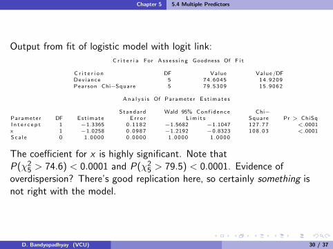
Output from fit of logistic model with logit link:
C r i t e r i a For A s s e s s i n g Goodness Of F i t
C r i t e r i o n DF Value Value /DFDev iance 5 74.6045 14.9209Pearson Chi−Square 5 79 .5309 15.9062
An a l y s i s Of Parameter E s t ima t e s
Standard Wald 95% Con f i d ence Chi−Parameter DF Est imate E r r o r L im i t s Square Pr > ChiSqI n t e r c e p t 1 −1.3365 0 .1182 −1.5682 −1.1047 127 .77 <.0001x 1 −1.0258 0 .0987 −1.2192 −0.8323 108 .03 <.0001Sca l e 0 1 .0000 0 .0000 1 .0000 1 .0000
The coefficient for x is highly significant. Note thatP(χ2
5 > 74.6) < 0.0001 and P(χ25 > 79.5) < 0.0001. Evidence of
overdispersion? There’s good replication here, so certainly something isnot right with the model.
D. Bandyopadhyay (VCU) 30 / 37
Chapter 5 5.4 Multiple Predictors
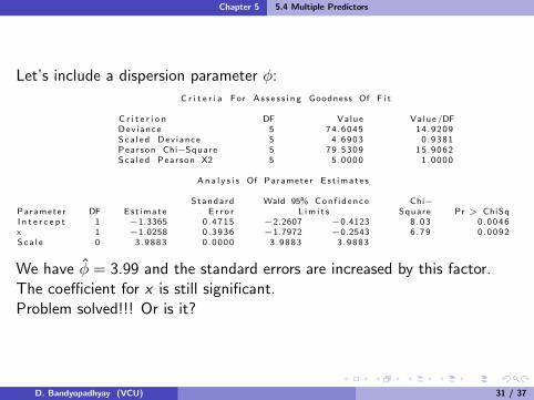
Let’s include a dispersion parameter φ:
C r i t e r i a For A s s e s s i n g Goodness Of F i t
C r i t e r i o n DF Value Value /DFDev iance 5 74.6045 14.9209Sca l ed Dev iance 5 4 .6903 0 .9381Pearson Chi−Square 5 79 .5309 15.9062Sca l ed Pearson X2 5 5.0000 1 .0000
An a l y s i s Of Parameter E s t ima t e s
Standard Wald 95% Con f i d ence Chi−Parameter DF Est imate E r r o r L im i t s Square Pr > ChiSqI n t e r c e p t 1 −1.3365 0 .4715 −2.2607 −0.4123 8 .03 0 .0046x 1 −1.0258 0 .3936 −1.7972 −0.2543 6 .79 0 .0092Sca l e 0 3 .9883 0 .0000 3 .9883 3 .9883
We have φ = 3.99 and the standard errors are increased by this factor.The coefficient for x is still significant.Problem solved!!! Or is it?
D. Bandyopadhyay (VCU) 31 / 37
Chapter 5 5.4 Multiple Predictors
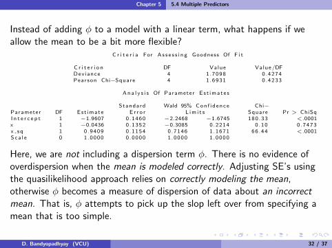
Instead of adding φ to a model with a linear term, what happens if weallow the mean to be a bit more flexible?
C r i t e r i a For A s s e s s i n g Goodness Of F i t
C r i t e r i o n DF Value Value /DFDev iance 4 1 .7098 0 .4274Pearson Chi−Square 4 1 .6931 0 .4233
An a l y s i s Of Parameter E s t ima t e s
Standard Wald 95% Con f i d ence Chi−Parameter DF Est imate E r r o r L im i t s Square Pr > ChiSqI n t e r c e p t 1 −1.9607 0 .1460 −2.2468 −1.6745 180 .33 <.0001x 1 −0.0436 0 .1352 −0.3085 0 .2214 0 .10 0 .7473x sq 1 0 .9409 0 .1154 0 .7146 1 .1671 66 .44 <.0001Sca l e 0 1 .0000 0 .0000 1 .0000 1 .0000
Here, we are not including a dispersion term φ. There is no evidence ofoverdispersion when the mean is modeled correctly. Adjusting SE’s usingthe quasilikelihood approach relies on correctly modeling the mean,otherwise φ becomes a measure of dispersion of data about an incorrectmean. That is, φ attempts to pick up the slop left over from specifying amean that is too simple.
D. Bandyopadhyay (VCU) 32 / 37
Chapter 5 5.4 Multiple Predictors
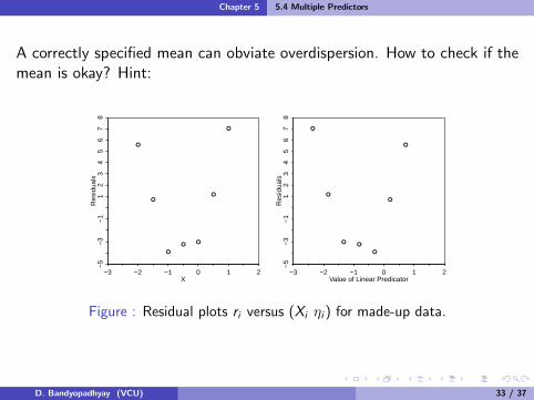
A correctly specified mean can obviate overdispersion. How to check if themean is okay? Hint:
●
●
●
●●
●
●
−3 −2 −1 0 1 2X
Res
idua
ls−
5−
3−
11
23
45
67
8
●
●
●
●●
●
●
−3 −2 −1 0 1 2Value of Linear Predicator
Res
idua
ls−
5−
3−
11
23
45
67
8
Figure : Residual plots ri versus (Xi ηi ) for made-up data.
D. Bandyopadhyay (VCU) 33 / 37
Chapter 5 5.4 Multiple Predictors
5.4.8 Estimating an Average Causal Effect
In many applications the explanatory variable of primary interestspecifies two groups to be compared while adjusting for the otherexplanatory variables in the model.
Let X1 = 0, 1 denote this two groups.
As an alternative effect summary to the log odds ratio β1, theestimated average causal effect is
1
n
∑i
[π(xi1 = 1, xi2, ..., xip)− π(xi1 = 0, xi2, ..., xip)]
Estimating an average causal effect is natural for experimentalstudies, and received much attention for non-randomized studies.
D. Bandyopadhyay (VCU) 34 / 37
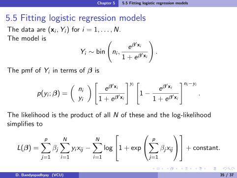
Chapter 5 5.5 Fitting logistic regression models
5.5 Fitting logistic regression modelsThe data are (xi ,Yi ) for i = 1, . . . ,N.The model is
Yi ∼ bin
(ni ,
eβ′xi
1 + eβ′xi
).
The pmf of Yi in terms of β is
p(yi ;β) =
(niyi
)[eβ′xi
1 + eβ′xi
]yi [1− eβ
′xi
1 + eβ′xi
]ni−yi.
The likelihood is the product of all N of these and the log-likelihoodsimplifies to
L(β) =
p∑j=1
βj
N∑i=1
yixij −N∑i=1
log
1 + exp
p∑j=1
βjxij
+ constant.
D. Bandyopadhyay (VCU) 35 / 37
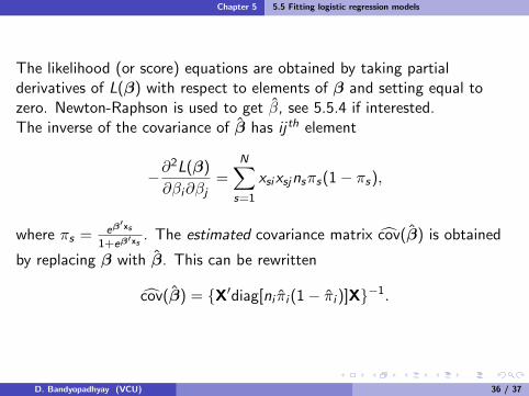
Chapter 5 5.5 Fitting logistic regression models
The likelihood (or score) equations are obtained by taking partialderivatives of L(β) with respect to elements of β and setting equal tozero. Newton-Raphson is used to get β, see 5.5.4 if interested.The inverse of the covariance of β has ij th element
−∂2L(β)
∂βi∂βj=
N∑s=1
xsixsjnsπs(1− πs),
where πs = eβ′xs
1+eβ′xs. The estimated covariance matrix cov(β) is obtained
by replacing β with β. This can be rewritten
cov(β) = {X′diag[ni πi (1− πi )]X}−1.
D. Bandyopadhyay (VCU) 36 / 37
Chapter 5 5.5 Fitting logistic regression models
Existence of finite β
Estimates β exist except when data are perfectly separated.
Complete separation happens when a linear combination of predictorsperfectly predicts the outcome. Here, there are an infinite number ofperfect fitting curves that have β =∞. Essentially, there is a value ofx that perfectly separates the 0’s and 1’s. In two-dimensions therewould be a line separating the 0’s and 1’s.
Quasi-complete separation happens when there’s a line that separates0’s and 1’s but there’s some 0’s and 1’s on the line. We’ll look atsome pictures.
The end result is that the model will appear to fit but the standarderrors will be absurdly large. This is the opposite of what’s reallyhappening, that the data can be perfectly predicted.
D. Bandyopadhyay (VCU) 37 / 37