14

CHAPTER 2SIMPLY-SUPPORTED CYLINDER STRUCTURAL RESPONSE

In this chapter the structural response of a simply-supported (SS) cylinder excited bypiezoelectric (PZT) actuators is addressed. Initially the theoretical formulation of Lalande’simpedance model of a PZT actuator exciting a SS cylinder is reviewed. The creation of a SSboundary condition on an actual cylinder is also described. The experimental results for thecreated cylinder are then presented and compared to the impedance model and finite elementanalysis results. The goal of the work presented here is to verify the analytical model of a SScylinder excited by PZT actuators. Once the model is validated, it can be used to predict thestructural response of a large scale cylinder which emulates a rocket payload fairing (PF).

2.1 PZT Actuator Model and Structural Response for a SS Cylinder

In this dissertation the structural response of a SS cylinder excited by PZT actuators isdetermined using the model developed by Lalande. This model was chosen because itincorporates the effects caused by the curvature of the actuators and the changing structuralimpedance of the cylinder as a function of frequency. Not considering the changing impedanceof the structure can lead to an incorrect predicted response (Lalande, 1995). Other models arediscussed in section 1.7. A brief overview of this model will now be presented.

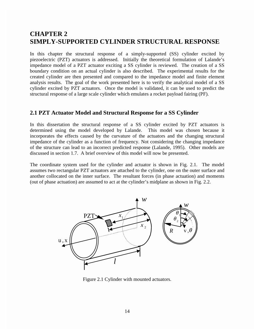
The coordinate system used for the cylinder and actuator is shown in Fig. 2.1. The modelassumes two rectangular PZT actuators are attached to the cylinder, one on the outer surface andanother collocated on the inner surface. The resultant forces (in phase actuation) and moments(out of phase actuation) are assumed to act at the cylinder’s midplane as shown in Fig. 2.2.

θ2

θ 1

l

x 2

x1

R

u x,

v ,θ

ww

PZT

Figure 2.1 Cylinder with mounted actuators.

15

Foutside

Finside

Nθ

Mθ

PZT

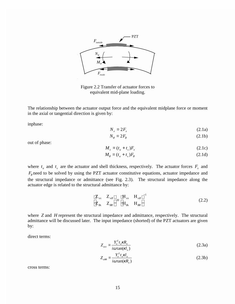
Figure 2.2 Transfer of actuator forces toequivalent mid-plane loading.

The relationship between the actuator output force and the equivalent midplane force or momentin the axial or tangential direction is given by:

inphase:N Fx x= 2 (2.1a)

N Fθ θ= 2 (2.1b)

out of phase:M t t Fx a s x= +( ) (2.1c)

M t t Fa sθ θ= +( ) (2.1d)

where ta and ts are the actuator and shell thickness, respectively. The actuator forces Fx and

Fθ need to be solved by using the PZT actuator constitutive equations, actuator impedance and

the structural impedance or admittance (see Fig. 2.3). The structural impedance along theactuator edge is related to the structural admittance by:

Z Z

Z Z

H H

H Hxx x

x

xx x

x

θ

θ θθ

θ

θ θθ

=

−1

(2.2)

where Z and H represent the structural impedance and admittance, respectively. The structuraladmittance will be discussed later. The input impedance (shorted) of the PZT actuators are givenby:

direct terms:

ZY t R

i laxxaE

a a

a

=κ

ω κtan( )(2.3a)

ZY t l

i RaaE

a a

a

θθ

κω κ

=tan( )

(2.3b)

cross terms:

16

ZY t l

i laxaE

a a

a

θ

κω κ

=tan( )

(2.3c)

ZY t R

i Ra xaE

a a

a

θ

κω κ

=tan( )

(2.3d)

where, YaE is the actuator complex modulus of elasticity with no applied electric field, Ra is the

actuator angular length, la is the actuator axial length, ω represents the angular frequency, i is

an imaginary number, and κ is given by:

κ ω ρ= a

aEY

(2.4)

where, ρ a is the density of the actuator.

u x,

v ,θ

FxFθ

Z xx

Zxθ

Zθθ

Z xθ

PZT

Ral a

Figure 2.3 Interaction between the PZT and the cylinder via the structural impedance.

Combining the actuator impedances, Eq. 2.3, with the PZT constitutive equations and applyingboundary conditions, a relationship between the dynamic actuator force and the structuralimpedance (Eq. 2.2) results (Zhou et al., 1993, Lalande, 1995):

( )Fi

RA l Z C R Z ex

a

a xx a xi t= − +ω κ κ θωsin( ) sin( ) (2.5a)

( )Fi

lA l Z C R Z e

a

a x ai t

θ θ θθωω κ κ= − +sin( ) sin( ) (2.5b)

where, A and C are calculated from,

A

C

lZ

Z

Z

Z

lZ

Z

Z

Z

a ax

ax

xx

axx

ax

axa

xx

axx

=

− +

−

κ κ ν

κ κ ν

θ

θ

θ

θ

cos( )

cos( )

1 κ κ ν

κ κ ν

θ

θ

θθ

θθ

θ

θ

θθ

θθ

cos( )

cos( )

RZ

Z

Z

Z

RZ

Z

Z

Z

d

dE

ax

a xa

a

a ax

a x a

f

−

− +

−

1

1

31

32

(2.6)

where, ν a , d31 and d32 are the actuator Poisson ratio and PZT constants and E f is the applied

electric field. By using Eqs. 2.1 and 2.5, the actuator output forces and moments can be used to

17

determine the structural response assuming the structural impedance is known. The computationof the structural response and structural impedance shall be presented next.

To determine the structural response of the SS cylinder caused by the actuation of the PZTactuator, a modal expansion analysis is performed. The equations that describe the motion of thecylinder are based on Love’s equations for shell structures. The general equations have beenadapted to incorporate loading caused by the actuation of line moments or forces (Soedel, 1981).Subsequently, the equations are developed to incorporate the loading generated by PZT actuators(Zhou et al., 1993, Lalande et al., 1995).

For a cylinder, the natural orthogonal modes can be used to determine the forced response usingan infinite series:

u x t p t U x ei k iki t

k

( , , ) ( ) ( , )θ θ ω==

∞

∑1

(2.7)

where, the subscript i corresponds to the associated displacement (i.e. i = 3 represents transversedisplacement), p tk ( ) represents the modal participation factor and U xik ( , )θ is the spatial modeshape. For a SS cylinder the mode shape is given by (Soedel, 1981):

U x A x nk mnp1 ( , ) cos( ) cos( )θ α θ= (2.8a)

U x B x nk mnp2 ( , ) sin( )sin( )θ α θ= (2.8b)

U x C x nk mnp3 ( , ) sin( ) cos( )θ α θ= (2.8c)

α π= m

l (2.8d)

where subscripts m and n represent the modal indices and subscript p refers to one of the threeprincipal coordinates (1,2,3). After performing the standard modal expansion procedure to thedifferential equations (multiplying by the mode shape, integrating over the domain, and applyingorthogonality conditions), the modal participation factor can be determined by solving anordinary differential equation with a redefined forcing function:

p t p t F ek k k ki t

••+ =( ) ( )ω ω2 (2.9)

where, Fk is the a modified forcing function determined by the actuator forcing terms in thedifferential equation. The modified forcing function is defined in other references and notincluded here for brevity (Soedel, 1981). The solution to the modal participation factor can begiven in the form:

pF

kk

k

=−ω ω2 2

(2.10)

Note that an equivalent damping factor has not been included in this formulation but insteadshall be included as a structural damping term with the modulus of elasticity. Equations 2.8 and2.10 are then substituted into Eq. 2.7 to obtain the response of the cylinder. This analysis wasperformed by Lalande and the result leads to the structural response of the cylinder (Lalande etal., 1995, Lalande, 1995):

18

[w x t S nnmp

( , , ) ( cosθ ϑ θθ= −=

∞

=

∞

=∑∑∑

111

3

]C n C x exi t

θωθ αsin ) sin (2.11)

where,

ϑρ ω ω

=−

−

+

R

t N

A

C

N

ns s mnp mnp

mnp

mnp

x

* ( )2 2

B

C

N

R

M

R

N

R n

M

n

M n

Rmnp

mnp

xθ θ θ θ

α α αα

α

+ + + +

2 2

S n n

C n n

C x xx

θ

θ

θ θθ θα α

= −= −= −

sin sin

cos cos

cos cos

1 2

1 2

1 2

where, Nmnp* is the mode normalization constant:

inphase:

NRl A

C

B

Cn mmnp

mnp

mnp

mnp

mnp

* ,= + +

≠ ≠π

21 0 0

2 2

out of phase:

NRl B

Cn mmnp

mnp

mnp

* ,= +

≠ ≠π

21 0 0

2

The ratios A Cmnp mnp and B Cmnp mnp can be found in work by Soedel (Soedel, 1981). Finally the

structural impedance needs to be described. For two dimensional structures, the admittancematrix is given by (Lalande, 1995):

2 2

2

uw

xu

inphaseoutphase

x x

inphase

••

=

•−

− −ς∂

∂ς ∂∂ θ θ

w

xH F H F

outphasex x

xx x x

•

=

= − +

1

( ) (2.12a)

2 2

2

vw

Rv

inphaseoutphase

inphase

••

=

•−

− −ς ∂

∂θθ θ

ς ∂∂θ

θ θ

θ θθ θw

RH F H F

outphase

x x

•

=

= − +

1

( ) (2.12b)

where,

ς =+( )t ts a

2

2

Based on the structural admittance defined in Eq. 2.12, the direct structural admittances aredetermined by dividing the axial or angular velocity by the appropriate force, Fx or Fθ . Forbrevity, only Hxx is presented. The remainder of the admittances can be found in prior citations(Lalande et al., 1995, Lalande, 1995).

HR n

A

Cxxin mnp

mnpnmp

=−

+

=

∞

=

∞

=∑∑∑1

2 1

2

111

3

( )θ θχ ( )χ α

θ θθ θout

o o xnS n C n C

2 −

cos sin (2.13)

where,

19

χ ωρ ω ωin

s s

x

mnp mnp

Ri

t

C

N= −

−2

2 2* ( )

χ ωρ ω ωout

s s

s a

mnp mnp

x

Ri

t

t t

NC= −

+−

( )

( )*

2

2 22

where θ o refers to the actuator center. The structural admittance (Eq. 2.13) can now be usedwith Eq. 2.2 to determine the structural impedance, and therefore the actuator forces can bedetermined and substituted into Eq. 2.11 to determine the transverse displacement of thecylinder. It is the transverse velocity component of the cylinder that generates the acoustic field,and is what is of interest in this work.

2.2 Creation of the Cylinder Simply-Supported Boundary Condition

Many aerospace and structural dynamics problems are too difficult to model analytically withexacting detail. To determine the general behavior of a distributed parameter system, researchersapproximate complicated structures with simpler models such as beams, plates and cylinders.Idealized cylinders are used to approximate more complex structures such as airplane fuselagesand rocket payload fairings (Niezrecki and Cudney, 1997, Lester and Lefebvre, 1991, Bullmoreet al., 1987). Previously, Arnold and Warburton performed some experiments on small diametercylinders (97.8 mm diameter). They created a SS boundary condition by accurately machining asteel plate to fit the bore of the cylinder. The end-condition tolerance was found to be extremelycritical in obtaining results that are in fair agreement with the theory (Arnold and Warburton,1949). Sewall compared experiments on SS cylindrically curved panels with analysis. But noexperiments on cylinders were performed (Sewall, 1967). Koga also studied the effects ofboundary conditions on the free vibration of circular cylindrical shells. However, none of theboundary conditions he tested can be considered simply-supported (Koga, 1988). Presented inthis section are the steps taken in creating a physical boundary condition which approximates theideal boundary condition for a SS cylinder. A variety of physical boundary conditions are testedand compared to determine the supports that most closely resemble the ideal SS boundarycondition. The experimental results are compared to finite element analysis FEA (using thesoftware package I-DEAS) and to the analytical prediction based on Love’s shell theory.

2.2.1 Various Boundary Conditions Tested

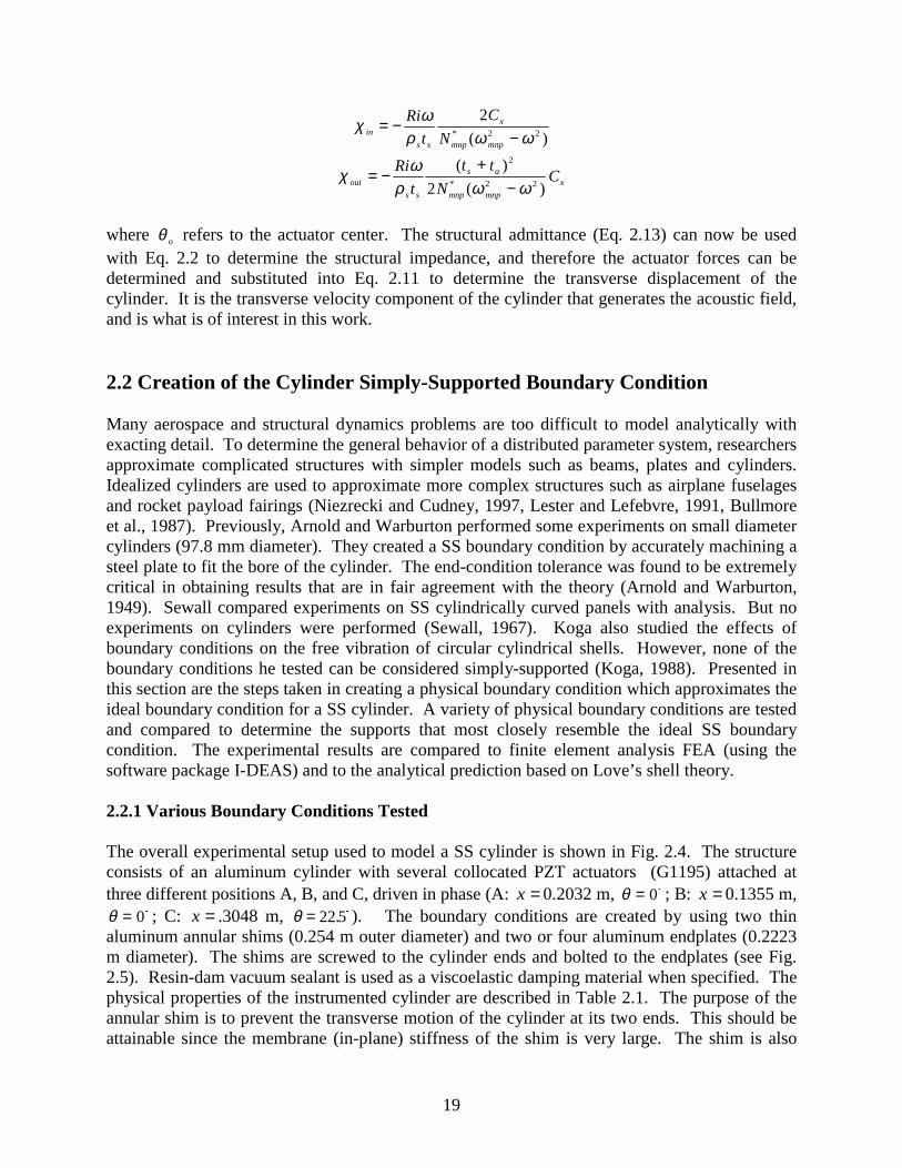
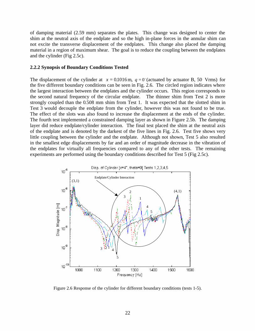
The overall experimental setup used to model a SS cylinder is shown in Fig. 2.4. The structureconsists of an aluminum cylinder with several collocated PZT actuators (G1195) attached atthree different positions A, B, and C, driven in phase (A: x =0.2032 m, θ = 0$ ; B: x =0.1355 m,θ = 0$ ; C: x = .3048 m, θ = 22 5. $ ). The boundary conditions are created by using two thinaluminum annular shims (0.254 m outer diameter) and two or four aluminum endplates (0.2223m diameter). The shims are screwed to the cylinder ends and bolted to the endplates (see Fig.2.5). Resin-dam vacuum sealant is used as a viscoelastic damping material when specified. Thephysical properties of the instrumented cylinder are described in Table 2.1. The purpose of theannular shim is to prevent the transverse motion of the cylinder at its two ends. This should beattainable since the membrane (in-plane) stiffness of the shim is very large. The shim is also

20

kept thin so the bending moment introduced by the shim at the cylinder edges is very small.Since the bending stiffness is proportional to the cube of the thickness, for a plate, the stiffness ofthe cylinder should be several orders of magnitude larger than that of the shim. Likewise for theendplate, compared to the shim. To create a test stand that approximates a SS boundarycondition, five different physical configurations were tested.

Figure 2.4 Instrumented cylinder.

Table 2.1 Cylinder and actuator properties

Property Cylinder PZT ActuatorYoung’s Modulus

(Pa) 64x109 63x109

Density (Kg/m3) 2700 7600Poisson’s Ratio 0.3 0.3

Loss Factor 0.005 0.001Length (mm) 406.4 38.1

Diameter (mm) 254 -Thickness (mm) 6.35 0.2413

Width (mm) - 31.5Applied Voltage - 50 or 25 Vrms

d32 (m/V) - -166x10-12

21

Cylinder

Shim

EndplateDamping

LayerConstrainingPlate

(a) (b)

Cylinder

Shim

DampingLayer

Endplates

(c)

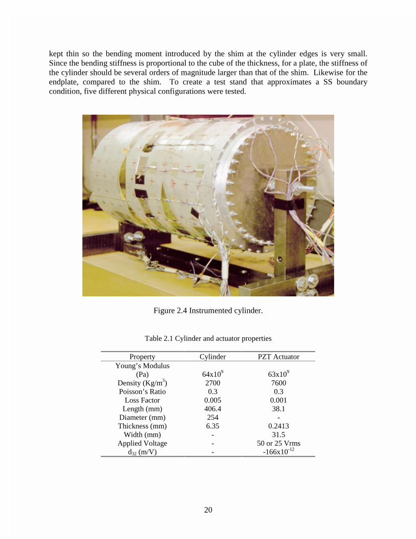
Figure 2.5 Tested boundary conditions: (a) test 1, 2, & 3: (b) test 4: (c) test 5.

Test 1: For the first test, the annular shim (0.508 mm thick) is screwed to the ends of the cylinderand is attached to a 12.7 mm thick circular endplate (Figure 2.5a).

Test 2: The setup is identical to Test 1 except a thinner annular shim (0.4064 mm) is used. Thischange was performed to see how altering the thickness (stiffness) of the shim affected theresponse.

Test 3: The setup is identical to Test 2 except the annular shim is now discontinuous and consistsof 18 individual radially sliced, slotted segments. Each of the individual segments contains aradial slot 9.525 mm deep (0.762 mm wide) on the outer and inner edge located at the middle ofthe segment. This change was performed to reduce the coupling between the endplates and thecylinder.

Test 4: The setup is identical to Test 1 except a layer of damping material (2.08 mm) has beenadded along with a circular constraining aluminum plate (0.2223 m diameter, 1.588 mm thick).The plate is bolted outside of the cylinder onto the endplates. This change was designed tointroduce some damping into the endplates and reduce their vibration (Figure 2.5b).

Test 5: The final setup used the same annular shim as in Test 1 except it is now beingsandwiched in the middle between two 6.35 mm thick aluminum endplates (four in all). A layer

22

of damping material (2.59 mm) separates the plates. This change was designed to center theshim at the neutral axis of the endplate and so the high in-plane forces in the annular shim cannot excite the transverse displacement of the endplates. This change also placed the dampingmaterial in a region of maximum shear. The goal is to reduce the coupling between the endplatesand the cylinder (Fig 2.5c).

2.2.2 Synopsis of Boundary Conditions Tested

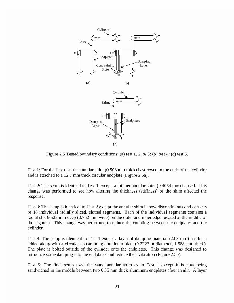
The displacement of the cylinder at x = 01016. m, θ = 0o (actuated by actuator B, 50 Vrms) forthe five different boundary conditions can be seen in Fig. 2.6. The circled region indicates wherethe largest interaction between the endplates and the cylinder occurs. This region corresponds tothe second natural frequency of the circular endplate. The thinner shim from Test 2 is morestrongly coupled than the 0.508 mm shim from Test 1. It was expected that the slotted shim inTest 3 would decouple the endplate from the cylinder, however this was not found to be true.The effect of the slots was also found to increase the displacement at the ends of the cylinder.The fourth test implemented a constrained damping layer as shown in Figure 2.5b. The dampinglayer did reduce endplate/cylinder interaction. The final test placed the shim at the neutral axisof the endplate and is denoted by the darkest of the five lines in Fig. 2.6. Test five shows verylittle coupling between the cylinder and the endplate. Although not shown, Test 5 also resultedin the smallest edge displacements by far and an order of magnitude decrease in the vibration ofthe endplates for virtually all frequencies compared to any of the other tests. The remainingexperiments are performed using the boundary conditions described for Test 5 (Fig 2.5c).

1

23

45

(3,1)

5

43 12

(4,1)

Endplate/Cylinder Interaction

Figure 2.6 Response of the cylinder for different boundary conditions (tests 1-5).

23

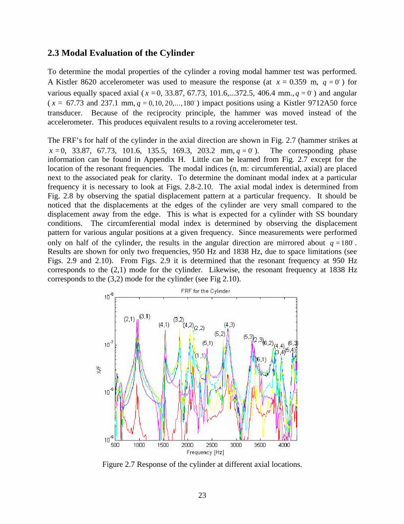
2.3 Modal Evaluation of the Cylinder

To determine the modal properties of the cylinder a roving modal hammer test was performed.A Kistler 8620 accelerometer was used to measure the response (at x = 0 359. m, θ = 0o ) forvarious equally spaced axial ( x = 0, 33.87, 67.73, 101.6,...372.5, 406.4 mm., θ = 0o ) and angular( x = 67.73 and 237.1 mm, θ = 0 10 20 180, , ,... , o ) impact positions using a Kistler 9712A50 forcetransducer. Because of the reciprocity principle, the hammer was moved instead of theaccelerometer. This produces equivalent results to a roving accelerometer test.

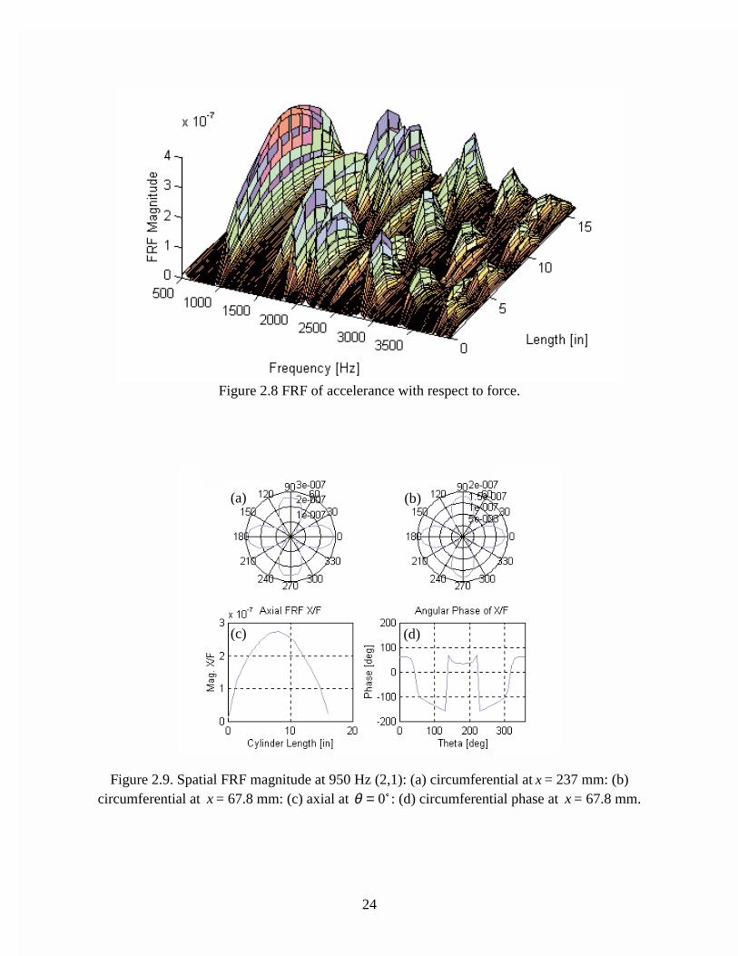
The FRF’s for half of the cylinder in the axial direction are shown in Fig. 2.7 (hammer strikes atx = 0, 33.87, 67.73, 101.6, 135.5, 169.3, 203.2 mm, θ = 0o ). The corresponding phaseinformation can be found in Appendix H. Little can be learned from Fig. 2.7 except for thelocation of the resonant frequencies. The modal indices (n, m: circumferential, axial) are placednext to the associated peak for clarity. To determine the dominant modal index at a particularfrequency it is necessary to look at Figs. 2.8-2.10. The axial modal index is determined fromFig. 2.8 by observing the spatial displacement pattern at a particular frequency. It should benoticed that the displacements at the edges of the cylinder are very small compared to thedisplacement away from the edge. This is what is expected for a cylinder with SS boundaryconditions. The circumferential modal index is determined by observing the displacementpattern for various angular positions at a given frequency. Since measurements were performedonly on half of the cylinder, the results in the angular direction are mirrored about θ = 180o .Results are shown for only two frequencies, 950 Hz and 1838 Hz, due to space limitations (seeFigs. 2.9 and 2.10). From Figs. 2.9 it is determined that the resonant frequency at 950 Hzcorresponds to the (2,1) mode for the cylinder. Likewise, the resonant frequency at 1838 Hzcorresponds to the (3,2) mode for the cylinder (see Fig 2.10).

Figure 2.7 Response of the cylinder at different axial locations.

24

Figure 2.8 FRF of accelerance with respect to force.

Figure 2.9. Spatial FRF magnitude at 950 Hz (2,1): (a) circumferential at x = 237 mm: (b)circumferential at x = 67.8 mm: (c) axial at θ = 0$ : (d) circumferential phase at x = 67.8 mm.

(a) (b)

(c) (d)

25

Figure 2.10 Spatial FRF at 1838 Hz (3,2): (a) circumferential at x = 237 mm: (b) circumferentialat x = 67.8 mm: (c) axial at θ = 0$ : (d) circumferential phase at x = 67.8 mm.

2.4 Comparison with Finite Element Analysis

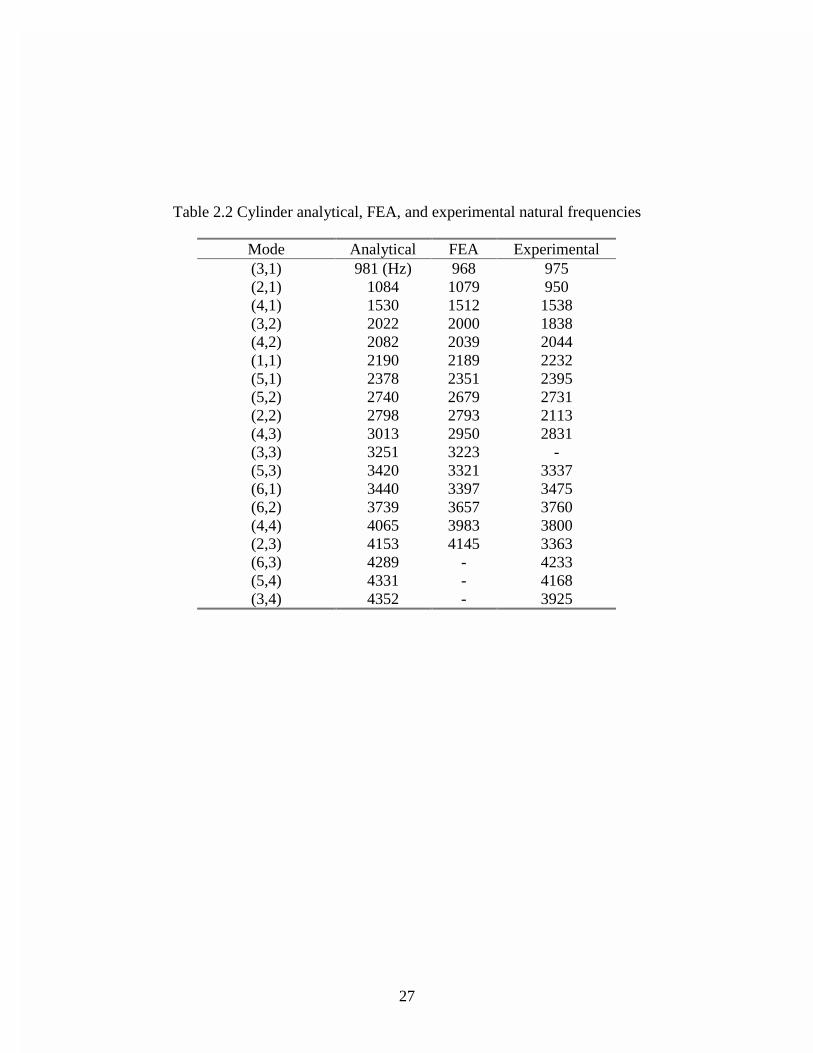
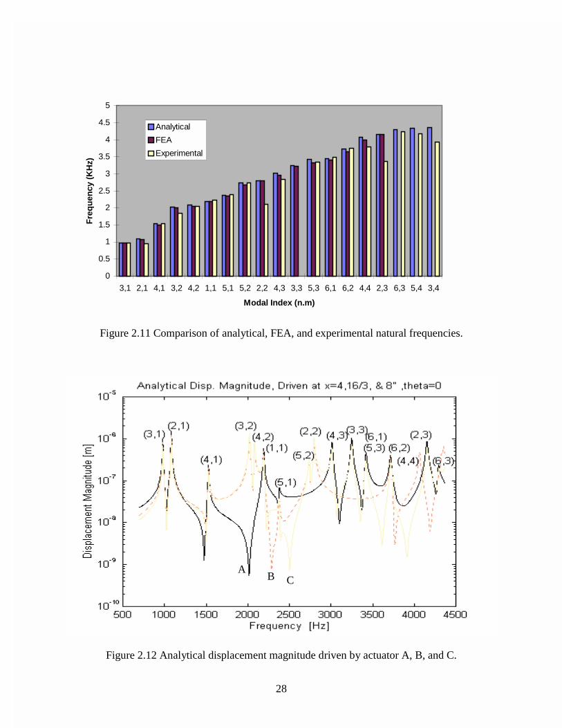
A finite element analysis (FEA) was also performed to compare with the natural frequenciesobtained analytically and experimentally for the cylinder. A finite element model was createdwith the software I-DEAS using 30 axial and 72 circumferential thin shell elements. The FEAmodel does not include any stiffening elements around the edge of the cylinder and is based on aSS boundary condition. The natural frequencies of the analytical model (based on Love’sequations), experimental natural frequencies, and frequencies predicted by FEA are shown inTable 2.2. The results are compared in Fig. 2.11.

It should be pointed out that in this work the cylinder’s resonant frequency is used toapproximate the location of the modal natural frequency. At a resonant frequency, the structuraloperating shape will be dominated by a particular mode at that frequency. Modal frequenciesand resonant frequencies of a structure are not necessarily the same. This is especially true if themodes are not well separated. If adjacent modes are close in frequency, then the operating shapewill be dominated by nearby modes. The operating shape has a contribution from all of themodes of a structure. Modes on the other hand are orthogonal and are essentially spatial basisfunctions that can be used in combination to describe the motion of the structure. The modalassurance criterion (MAC) is used in Appendix I to show the limitations of this approximation.

The analytical and FEA natural frequencies have an overall relative difference of 1.32% for thesixteen modes. The deviation between the analytical and experimental natural frequenciesranges from 0.5 to 24.5% depending on the mode. The major difference occurs in the two andthree circumferential modes for the tested frequency range. It is believed that this deviation iscaused because of the close proximity of the second (1200 Hz) and third (3850 Hz) modes of the

(a) (b)

(c) (d)

26

endplate. In general the analytical and experimental modes of the cylinder share the samemodal order and are relatively close. The SS cylinder created to model an ideal SS cylinder isclearly not perfect. It does however have very similar vibrating properties and modaldistribution. It should be pointed out that the cylinder is not perfectly uniform on its exteriorsurface. This is due to several other mounted PZT actuators and milled flats which were used fora previous experiment (Sumali, 1992). It is believed that these effects are minimal and shouldnot significantly affect the vibrating properties of the cylinder.

2.5 Response to Various Actuator Locations

To help verify the response of the cylinder to excitation at different locations, the cylinder isexcited at different positions and the response is compared (A: x =203.2 mm, θ = 0$ ; B:x =135.5 mm, θ = 0$ ; C: x =304.8 mm, θ = 22 5. $ ). Actuator A, B, and C are used to excite thecylinder at 25 Vrms using a sine-dwell test over a broad frequency range measured at x = 338.7

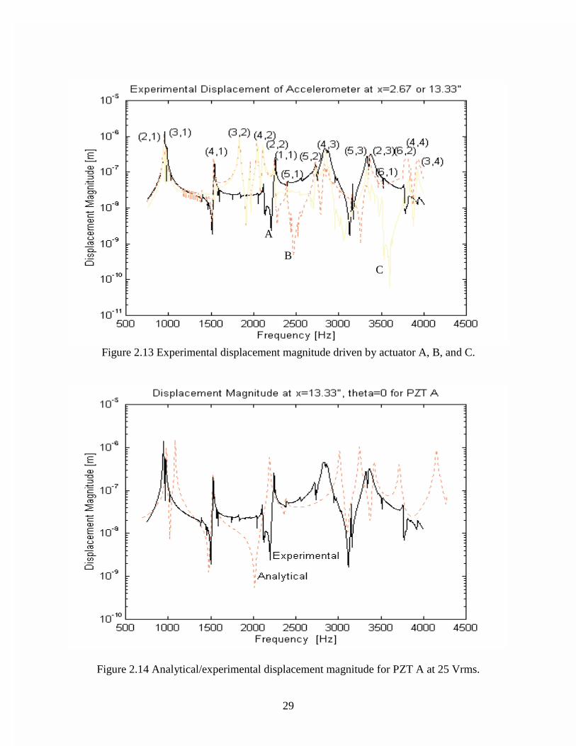
mm θ = 0$ for actuator A and B and x =67.73 mm, θ = 22 5. $ for actuator C. The analytical andexperimental results are shown in Figs. 2.12 and 2.13, respectively. For actuator A, theanalytical model predicts the actuator will strongly excite the odd axial modes and ignore theeven axial modes. This makes physical sense since actuator A is located at the center of thecylinder and is verified by Fig. 2.13. For actuator B, the analytical model predicts the actuatorwill excite the odd axial modes and will ignore the three axial modes. Similar trends are seen inFig 2.13. Lastly, the actuator located ¼ of the length of the cylinder, actuator C, is predicted toexcite the axial two modes the most. This is also confirmed by the experiment. An exception tothis general behavior occurs at the (6,2) mode where it is expected that actuator A should notproduce any excitation. However, both the analysis and experiment show a strong coupling atthat frequency. The overall analytical response follows the expected physical trends withrespect to actuator location and is similar to the experimental results.

2.6 Analytical and Experimental Response

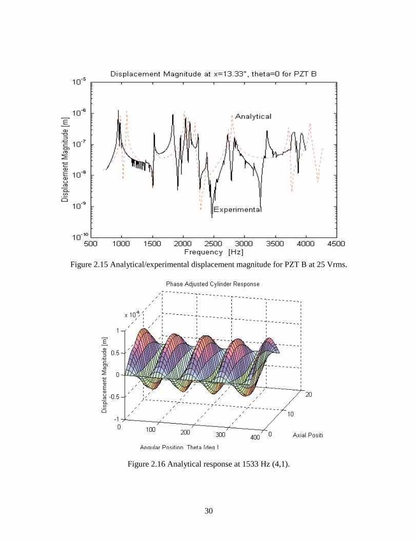
Presented in Figs. 2.14 and 2.15 are the analytical and experimental response of the cylinder foractuator A and B measured at x = 338.7 mm, θ = 0$ . The relative magnitude of the predictedresponse is within half an order of magnitude compared to the measured response using anoverall structural damping value of 0.5% (the predicted response magnitude depends on thedamping value). Even though the frequencies of some modes are shifted, the dominant behaviorof the cylinder is predicted by the model and the relative magnitudes are reasonably close.

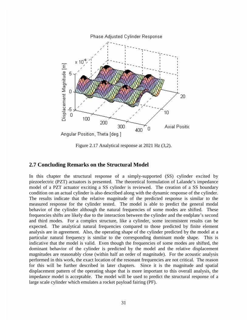
For the analytical natural frequencies, which correspond to the (4,1) and (3,2) modes, theanalytical spatial displacement response is shown in Figs. 2.16 and 2.17. The response of thecylinder has been unwrapped and so results can be more easily plotted. The phase of thedisplacement response has been incorporated into the plots to show actual normal displacements.As is expected for each of these frequencies, the predicted operating shape is similar to thedominant mode. The results indicate that the impedance model for PZT’s actuating a SScylinder can approximate the overall resonant and modal behavior.

27

Table 2.2 Cylinder analytical, FEA, and experimental natural frequencies

Mode Analytical FEA Experimental(3,1) 981 (Hz) 968 975(2,1) 1084 1079 950(4,1) 1530 1512 1538(3,2) 2022 2000 1838(4,2) 2082 2039 2044(1,1) 2190 2189 2232(5,1) 2378 2351 2395(5,2) 2740 2679 2731(2,2) 2798 2793 2113(4,3) 3013 2950 2831(3,3) 3251 3223 -(5,3) 3420 3321 3337(6,1) 3440 3397 3475(6,2) 3739 3657 3760(4,4) 4065 3983 3800(2,3) 4153 4145 3363(6,3) 4289 - 4233(5,4) 4331 - 4168(3,4) 4352 - 3925

28

0

0.5

1

1.5

2

2.5

3

3.5

4

4.5

5

3,1 2,1 4,1 3,2 4,2 1,1 5,1 5,2 2,2 4,3 3,3 5,3 6,1 6,2 4,4 2,3 6,3 5,4 3,4

Modal Index (n.m)

Fre

qu

ency

(K

Hz)

Analytical

FEA

Experimental

Figure 2.11 Comparison of analytical, FEA, and experimental natural frequencies.

Figure 2.12 Analytical displacement magnitude driven by actuator A, B, and C.

AB C

29

Figure 2.13 Experimental displacement magnitude driven by actuator A, B, and C.

Figure 2.14 Analytical/experimental displacement magnitude for PZT A at 25 Vrms.

A

BC

30

Figure 2.15 Analytical/experimental displacement magnitude for PZT B at 25 Vrms.

Figure 2.16 Analytical response at 1533 Hz (4,1).

31

Figure 2.17 Analytical response at 2021 Hz (3,2).

2.7 Concluding Remarks on the Structural Model

In this chapter the structural response of a simply-supported (SS) cylinder excited bypiezoelectric (PZT) actuators is presented. The theoretical formulation of Lalande’s impedancemodel of a PZT actuator exciting a SS cylinder is reviewed. The creation of a SS boundarycondition on an actual cylinder is also described along with the dynamic response of the cylinder.The results indicate that the relative magnitude of the predicted response is similar to themeasured response for the cylinder tested. The model is able to predict the general modalbehavior of the cylinder although the natural frequencies of some modes are shifted. Thesefrequencies shifts are likely due to the interaction between the cylinder and the endplate’s secondand third modes. For a complex structure, like a cylinder, some inconsistent results can beexpected. The analytical natural frequencies compared to those predicted by finite elementanalysis are in agreement. Also, the operating shape of the cylinder predicted by the model at aparticular natural frequency is similar to the corresponding dominant mode shape. This isindicative that the model is valid. Even though the frequencies of some modes are shifted, thedominant behavior of the cylinder is predicted by the model and the relative displacementmagnitudes are reasonably close (within half an order of magnitude). For the acoustic analysisperformed in this work, the exact location of the resonant frequencies are not critical. The reasonfor this will be further described in later chapters. Since it is the magnitude and spatialdisplacement pattern of the operating shape that is more important to this overall analysis, theimpedance model is acceptable. The model will be used to predict the structural response of alarge scale cylinder which emulates a rocket payload fairing (PF).