Calculation of receiver sensitivity

( ) Ao

o rms Tv

v KT rms

∂∂ ∆°∆

where Ao Tv ∂∂

calibrates voltage as temperature

oDCo v)f( ⇒Φ

rmsoACo v)f( ⇒Φ

Approach:

)f()f()t(

)t(v

odd

d

Φ↔φ

↓

↔ ?

t

vo(t) compressed time vrms → ∆Trms

( )RAo TTv +∝

ov

0

Receivers-B1

TA + TR

Φ ⇒

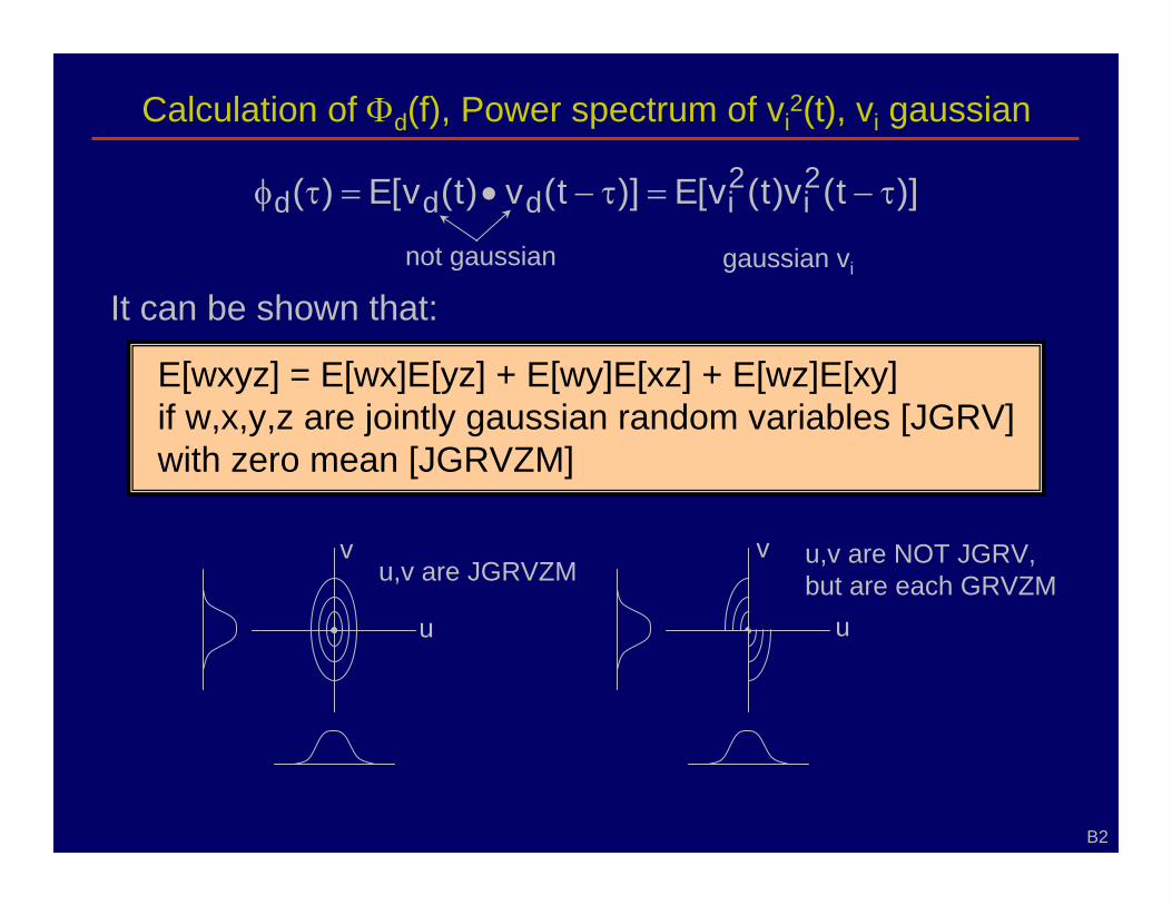
Calculation of Φd(f), Power spectrum of vi 2(t), vi gaussian

)]t(v)t(v[E)]t(v)t(v[E)( 2 i

2 iddd =•=τφ

not gaussian gaussian vi

It can be shown that:

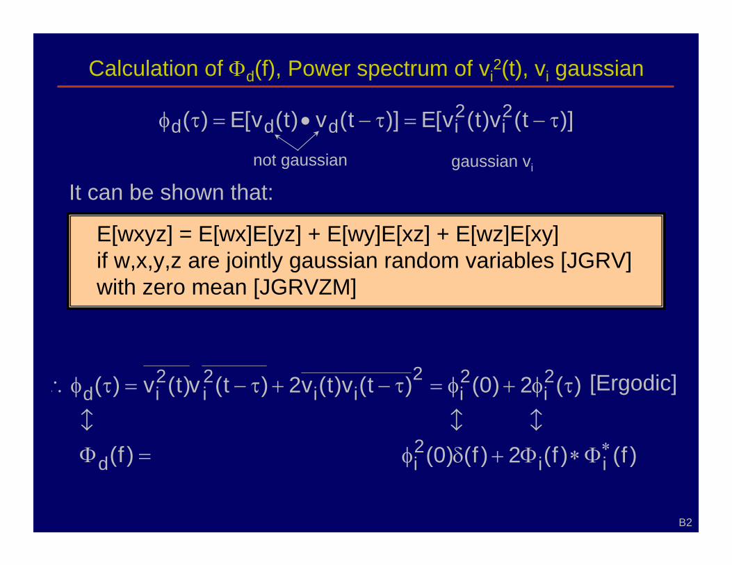
E[wxyz] = E[wx]E[yz] + E[wy]E[xz] + E[wz]E[xy] if w,x,y,z are jointly gaussian random variables [JGRV] with zero mean [JGRVZM]

B2

v

u

v

u

u,v are JGRVZM u,v are NOT JGRV, but are each GRVZM

τ − τ −

Calculation of Φ d(f), Power spectrum of vi 2(t), vi gaussian

)]t(v)t(v[E)]t(v)t(v[E)( 2 i

2 iddd =•=τφ

not gaussian gaussian vi

It can be shown that:

E[wxyz] = E[wx]E[yz] + E[wy]E[xz] + E[wz]E[xy] if w,x,y,z are jointly gaussian random variables [JGRV] with zero mean [JGRVZM]

)(2)0()t(v)t()t(v)t(v)( 2 i

2 i

2 ii

2 i

2 id τφ+=τφ∴ [Ergodic]

=Φ )f(d )f()f(2)f()0( ii 2 i

∗Φ+δφ

7 7 7

B2

τ − τ −

v 2 φ = τ − + τ −

Φ ∗

)f()f(2)f()0()f( ii 2 id

∗Φ+δΦ

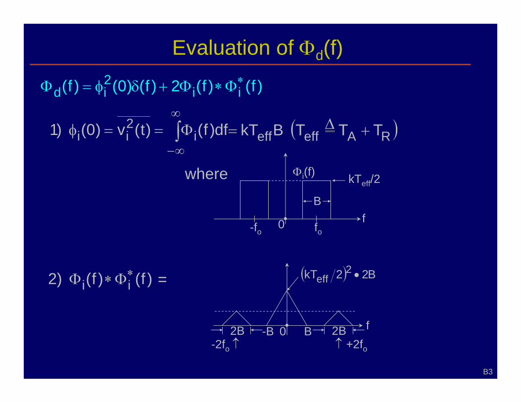
Evaluation of Φ d(f)

∫ ∞

∞−

Φ==φ df)f()t(v)0()1 i 2 ii ( ) RAeffeff TTTBkT +∆=

where

-fo 0

B f

kTeff/2Φ i(f)

)f()f(2) ii ∗Φ

-B B0 f2B2B

( ) 2kT 2 eff •

-2fo ↑ ↑ +2fo

=

fo

B3

Φ ∗ φ =

Φ ∗ B2

)f()f(2)f()0()f( ii 2 id

∗Φ+δΦ

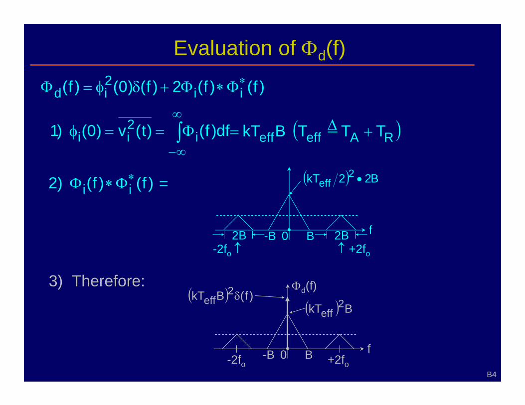
Evaluation of Φ d(f)

∫ ∞

∞−

Φ==φ df)f()t(v)0()1 i 2 ii ( ) RAeffeff TTTBkT +∆=

)f()f(2) ii ∗Φ

-B B0 f2B2B

( ) 2kT 2 eff •

-2fo ↑ ↑ +2fo

=

3) Therefore:

-B B0 f

( ) BkT 2 eff

-2fo +2fo

Φ d(f)( ) )f(BkT 2 eff δ

B4

Φ ∗ φ =

Φ ∗ B2

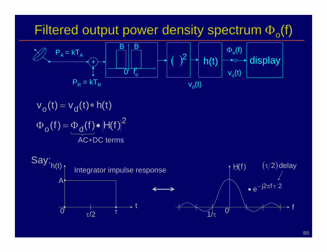
Filtered output power density spectrum Φ o(f)

+ 0

BB PA = kTA ( ) 2 h(t) display

PR = kTR

2 do

do

)f(H)f()f(

)t(h)t(v)t(v

•Φ=Φ

∗=

AC+DC terms

Say:h(t)

A

0 t

ττ /2

Integrator impulse response

fo

vd(t)

Φ o(f)

vo(t)

)f(H

2je τπ−•

( )τ

1/τ 0 f

B5

f 2

delay 2

2 do

do

)f(H)f()f(

)t(h)t(v)t(v

•Φ=Φ

∗=

AC+DC terms Say:h(t)

A

0 t

ττ /2

Integrator impulse response

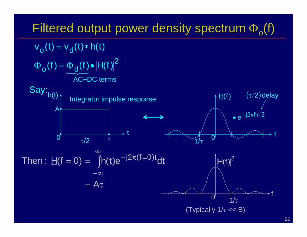
)0f( =

τ=

= ∫ ∞

=π−

A

dte)t(h t)0f(2j 2)f(H

f0 1/τ (Typically 1/τ << B)

Filtered output power density spectrum Φ o(f)

)f(H

2je τπ−•

( )τ

1/τ 0 f

B6

H : Then ∞ −

f 2

delay 2

( ) ( )

( ) ∫∫ ∞

∞−

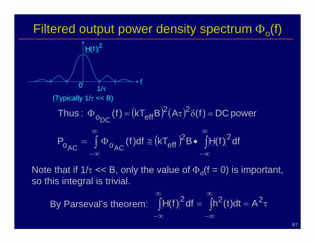
∞ •≅Φ=

=δτ=Φ

df)f(HBkTdf)f(P

)f(ABkT)f(

22 effoo

22 effo

ACAC

DC

Note that if 1/τ << B, only the value of Φ d(f = 0) is important, so this integral is trivial.

By Parseval’s theorem: τ== ∫∫ ∞

∞−

∞

∞−

222 Adt)t(hdf)f(H

2)f(H

f0 1/τ (Typically 1/τ << B)

Filtered output power density spectrum Φ o(f)

B7

∞ −

power DC : Thus

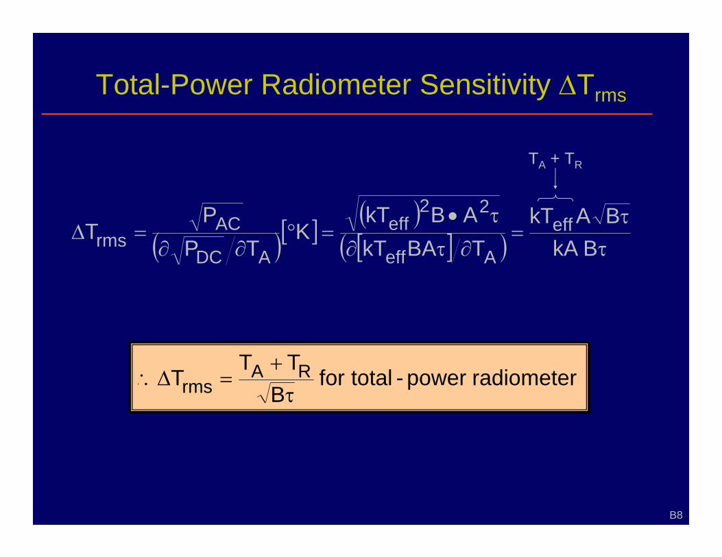
Total-Power Radiometer Sensitivity ∆ Trms

( ) [ ] ( ) [ ]( ) τ

τ =

∂

τ• =°

∂∂ =∆

BAkT TBAkT

ABkTK

TP P

T eff

Aeff

22 eff

ADC

AC rms

TA + TR

-B

TTT RA

rms τ +

=∆∴

B8

∂ τ B kA

radiometer power total for

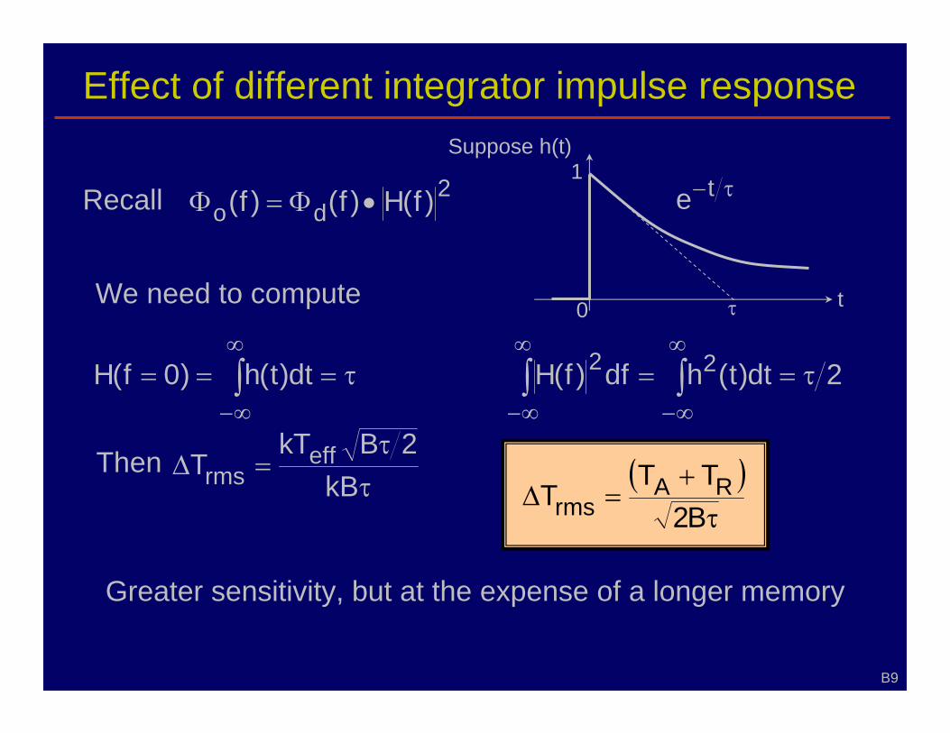
Effect of different integrator impulse response

2 do )f(H)f()f( •Φ=ΦRecall

We need to compute

== ∫ ∞

dt)t(h)0f(H

Then τ τ

=∆ kB

2BkTT eff

rms

2dt)t(hdf)f(H 22 = ∫∫ ∞

∞−

∞

∞−

Suppose h(t)

0 τ t

1 τ− te

Greater sensitivity, but at the expense of a longer memory

( ) τ

+ =∆

TTT RA

rms

B9

τ = ∞ −

τ =

B2

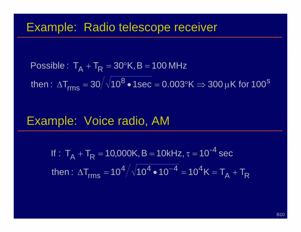
Example: Radio telescope receiver

Example: Voice radio, AM

s8 rms

RA

3001030T

T

µ⇒°=•=∆

=°=+

RA 4444

rms

RA

TT101010T

sec1010kHz,Tf

+==•=∆

==+

−

B10

100 for K K 003. 0 sec1 : then

MHz 100 B ,K 30 T : Possible

4 ­

K 10 : then

B ,K000,10 T : I = τ

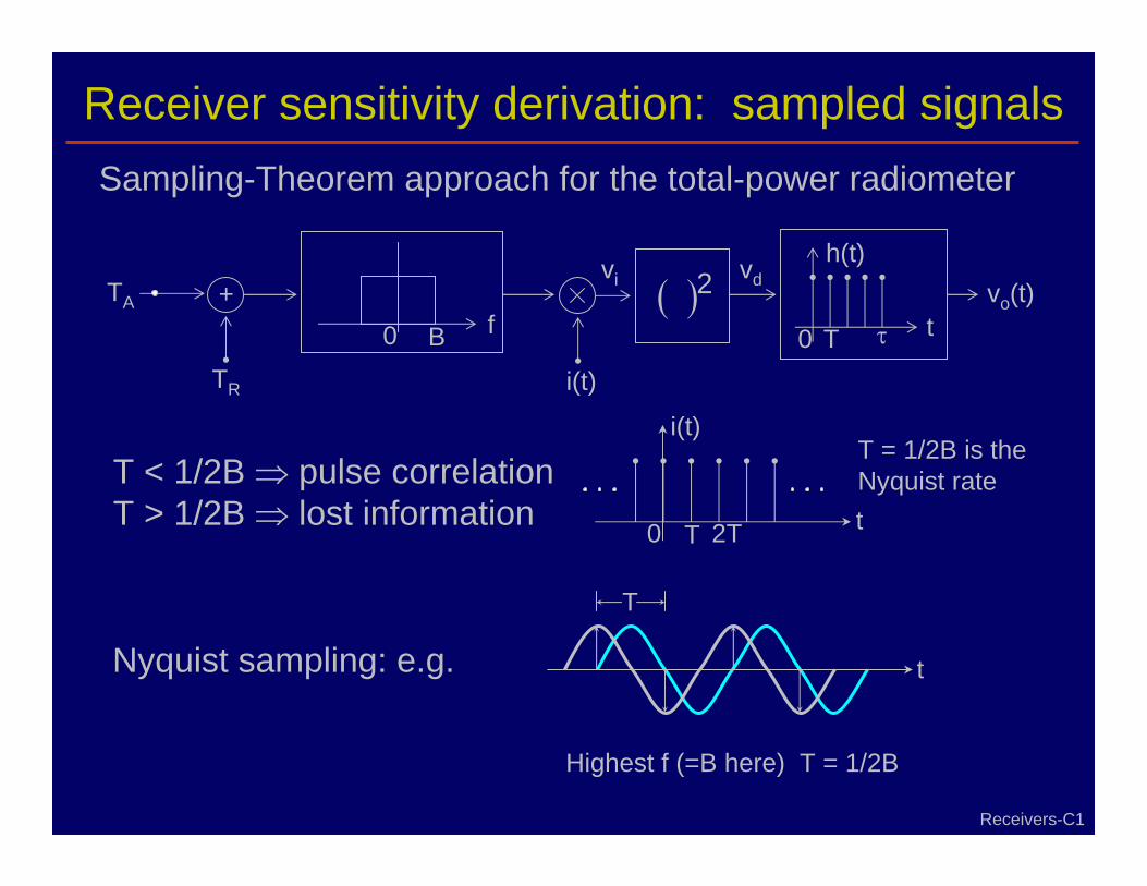
Receiver sensitivity derivation: sampled signals Sampling-Theorem approach for the total-power radiometer

Nyquist sampling: e.g.

T

t

Highest f (=B here) T = 1/2B

0 B f ( )2

0 T t

h(t)

τ

vo(t)TA

TR i(t)

vi vd +

T < 1/2B ⇒ pulse correlation T > 1/2B ⇒ lost information 0 T 2T t

T = 1/2B is the Nyquist rate

i(t)

Receivers-C1

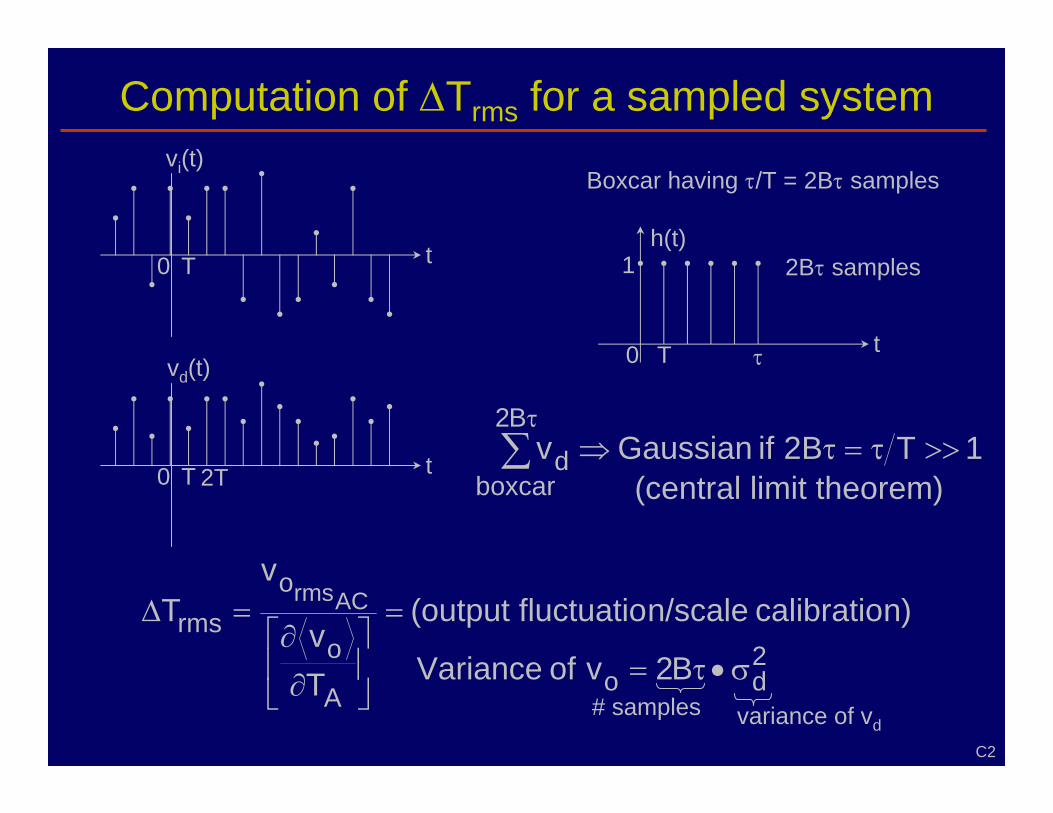
Computation of ∆ Trms for a sampled system

Boxcar having τ /T = 2Bτ samples

0 tT

0 tT 2T 1Tv

boxcar d >>⇒∑

τ

0 T τ t

h(t) 1

T v

v T

A

o

o rms

ACrms =

⎥ ⎦

⎤ ⎢ ⎣

⎡

∂

∂ =∆

2 do =

# samples variance of vd

vi(t)

2Bτ samples

vd(t)

(central limit theorem)

C2

2B if Gaussian B2

τ = τ

n) calibratio n/scale fluctuatio (output

B2 v of Variance σ • τ

T v

v T

A

o

o rms

ACrms =

⎥ ⎦

⎤ ⎢ ⎣

⎡

∂

∂ =∆

2 do τ=

# samples variance of vd

( ) ( ) 22 i

2 i

2 dd

2 d vvvv −=−∆σ (where vi = JGRVZM)

( ) ( ) ( ) 22 i

4 i

22 i

22 i

4 i vvvv −=+−=

)xaT 2 eff

2 i

2 ••=≡

)1n(5 nn =−• •••= (where x = JGRVZM)

( ) N N 22

eff

2

1

2

3

422 eff

22 i

4 i

2 d axxaTvv =

⎥ ⎥

⎦

⎤

⎢ ⎢

⎣

⎡

⎟ ⎟ ⎠

⎞ ⎜ ⎜ ⎝

⎛ −=−=σ

22 effo a• τ=

C3

n) calibratio n/scale fluctuatio (output

B2 v of Variance σ •

v 2

a" " defines equation (this v and here 1 x : Let

odd n if ,0 x even; if ,3 1 x : Recall

T2 : Thus

T2 B2 v of variance the and

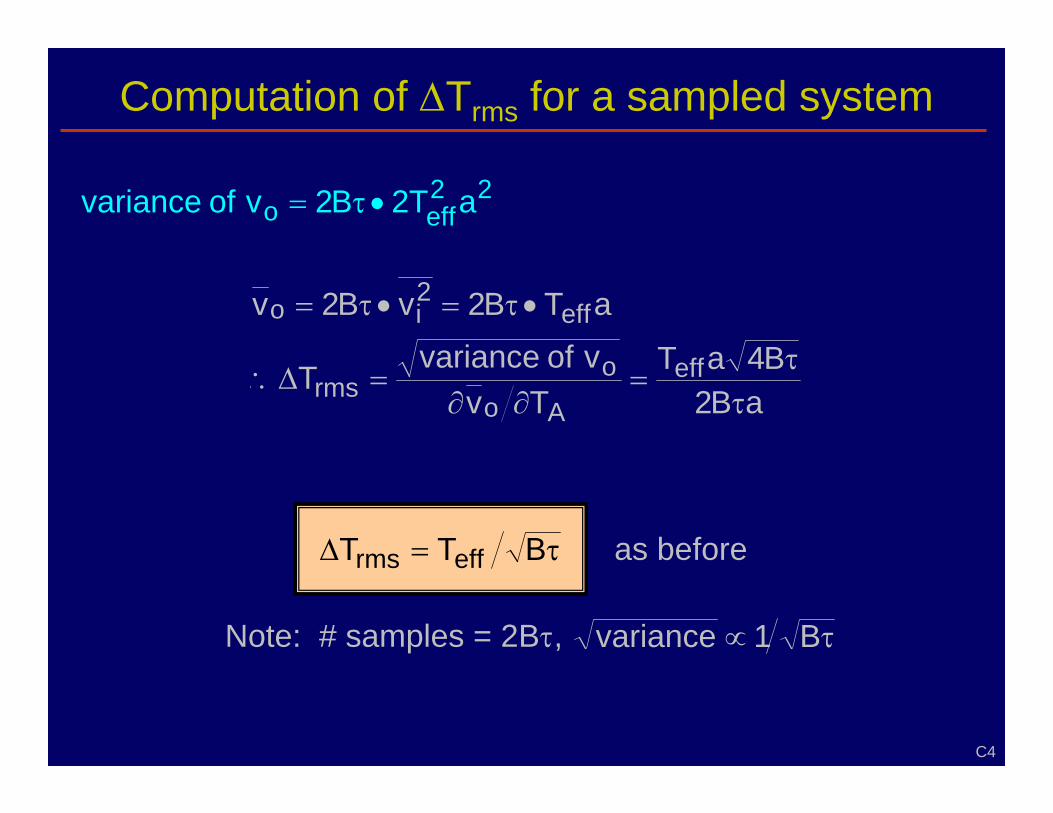
22 effo a• τ=

aT Tv

T

aTvv

eff

Ao o

rms

eff 2 io

τ τ

= ∂∂

=∆∴

• τ=• τ=

τ=∆ BTT effrms as before

Note: # samples = 2Bτ , τ∝ B1variance

Computation of ∆ Trms for a sampled system

C4

T2 B2 v of variance

a B2 B4 v of variance

B2 B2

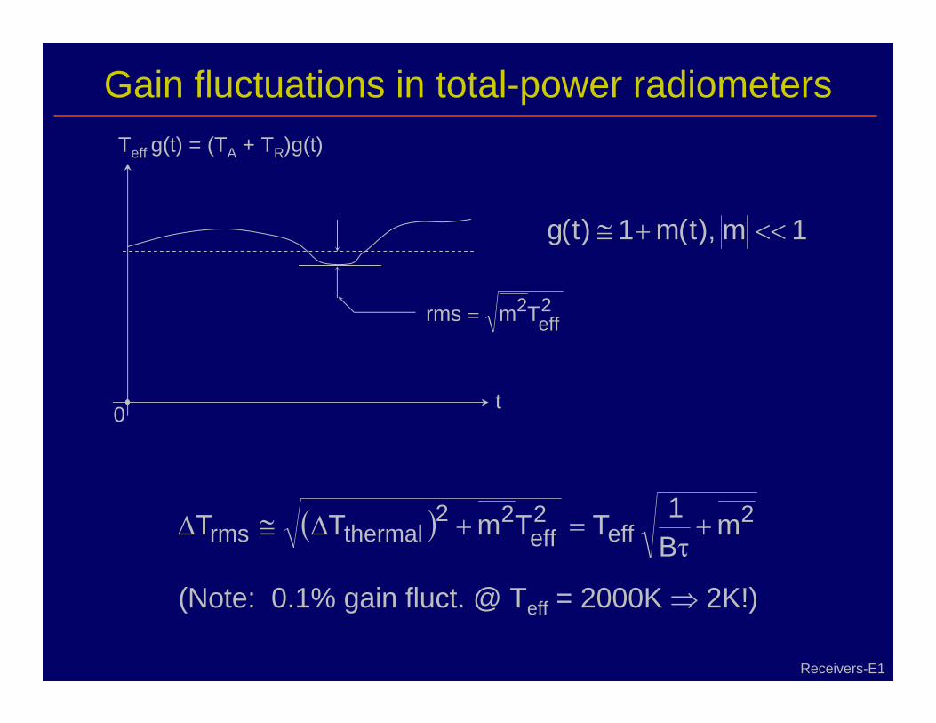
Gain fluctuations in total-power radiometers

( ) 2 eff

2 eff

22 thermalrms m

B 1TTT + τ

=+∆≅∆

(Note: 0.1% gain fluct. @ Teff = 2000K ⇒ 2K!)

1(m1)t(g < <+≅

Teff g(t) = (TA + TR)g(t)

2 eff

2rms =

0 t

Receivers-E1

T m

m ), t

T m

One solution to gain variations: “Synchronous detection”

Dicke radiometer

receiver

∫

∫TA

TCAL

Zo

TR vo(t) +

-

vSD(t) ∝ TA - TCAL

vo(t)

0 t

integrated by upper integrator integrated by lower integrator

= rmsSDv unchanged (looking at same signal all the time)

but =∂∂ effSD Tv

BT effrmsDicke τ=∆∴

former value (we view TA half the time)2 1

~VSD Note: gain is irrelevant

when TA = TC

∝ (TR + TA)

∝ (TR + TC)

E2

only) null (at T2

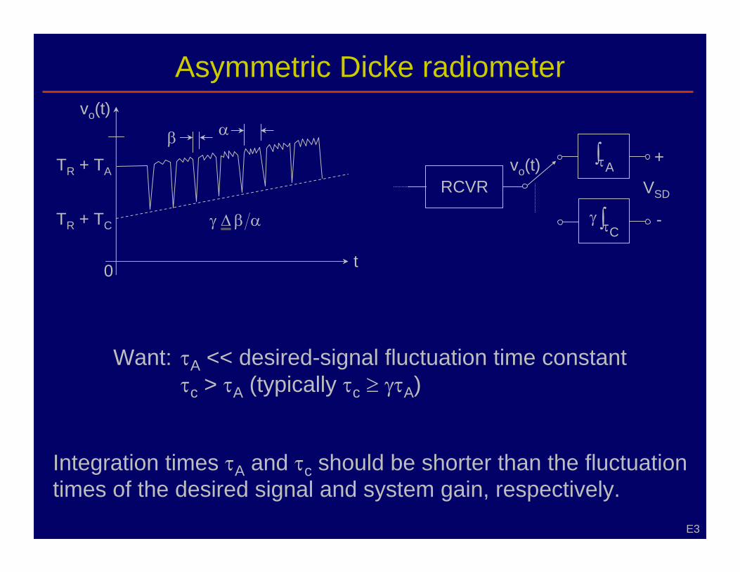
Asymmetric Dicke radiometer

Integration times τ A and τ c should be shorter than the fluctuation times of the desired signal and system gain, respectively.

Want: τ A << desired-signal fluctuation time constant τ c > τ A (typically τ c ≥ γ τ A)

vo(t)

TR + TA

TR + TC

RCVR

∫ τ A

∫ τγ C

+

-

VSD

vo(t)

t0

αβ∆γ

β α

E3

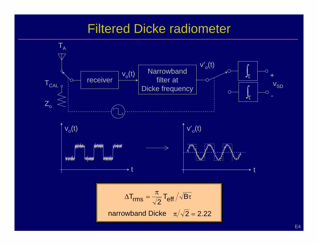
Filtered Dicke radiometer

receiver Narrowband

filter at Dicke frequency

vo(t) v’o(t) ∫τ

∫τ

+

-

TCAL

Zo

TA

vo(t) o(t)

t t

τπ

=∆ BT 2

T effrms

narrowband Dicke 2 =π

vSD

E4

v’

22. 2

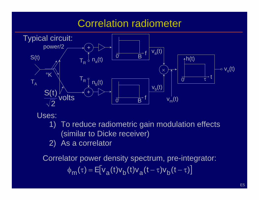
Correlation radiometer

Uses:

Correlator power density spectrum, pre-integrator: [ ] )t(v)t(v)t(v)t()( babam τ−=τφ

Typical circuit:

0 t

h(t)

τ

×

+ B0 f

+ B0 f

S(t)

TA

°K

TR

TR

na(t)

nb(t) vb(t)

va(t)power/2

vm(t)volts2 )t(S

vo(t)

E5

1) To reduce radiometric gain modulation effects (similar to Dicke receiver)

2) As a correlator

v E τ −

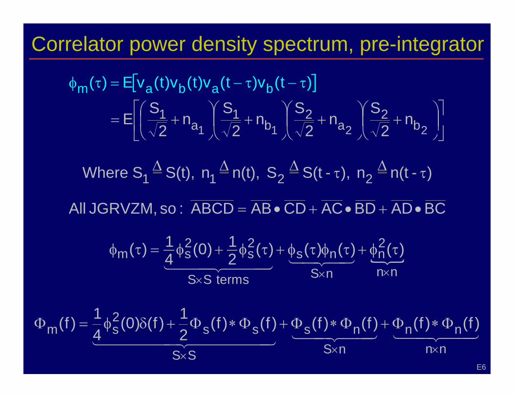
Correlator power density spectrum, pre-integrator

[ ])t(v)t(v)t(v)t()( babam τ−τ−=τφ

⎥⎦

⎤ ⎢⎣

⎡ ⎟ ⎠

⎞⎜ ⎝

⎛ +⎟ ⎠

⎞⎜ ⎝

⎛ +⎟ ⎠

⎞⎜ ⎝

⎛ +⎟ ⎠

⎞⎜ ⎝

⎛ += 2211 b

2 a

2 b

1 a

1 n2

S n

2 S

n2

S n

2 S

E

)2211 τ∆τ∆∆∆

BCADBDACCDAB •+•+•=

N 2 2 2

m s s s n n n nS n

1 1( ) (0) ( ) ( ) ( ) ( )4 2 ×××

φ τ = φ + φ τ

�������� nnnsss

2 sm )f()f()f()f()f()f(

2 1)f()0(

4 1)f(

×××

Φ+δφ=Φ

E6

v E

-n(t n ), -S(t S n(t), n S(t), S Where

ABCD : so JGRVZM, All

S S terms

τ + φ τ φ τ + φ ����������

�� �� ����� ���� n n n S S S

Φ ∗ Φ + Φ ∗ Φ + Φ ∗

�������� nnnsss

2 sm )f()f()f()f()f()f(

2 1)f()0(

4 1)f(

×××

Φ+δφ=Φ

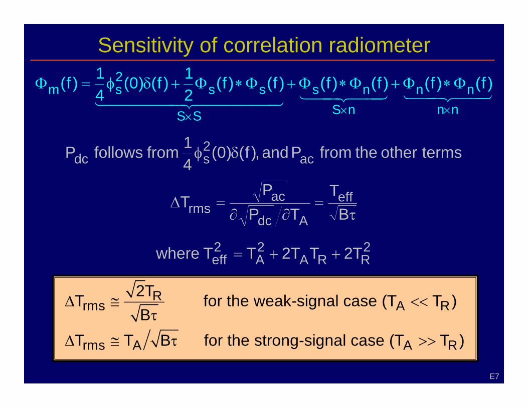
Sensitivity of correlation radiometer

)f()0(4 1P ac

2 sdc δφ

τ =

∂∂ =∆

B T

TP P

T eff

Adc

ac rms

2 RRA

2 A

2 eff T ++=

R A R

A A R

2TT i (T T )B

T T B i (T T )

∆ ≅ τ

∆ ≅ τ

E7

�� �� ����� ���� n n n S S S

Φ ∗ Φ + Φ ∗ Φ + Φ ∗

terms other the from P and ,from follows

T2 T T2 T where

rms

rms

for the weak-s gnal case

for the strong-s gnal case

< <

> >

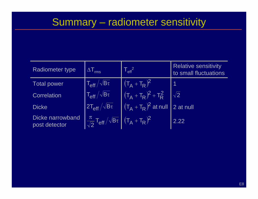
Summary – radiometer sensitivity

Radiometer type ∆Trms Teff 2 Relative sensitivity

to small fluctuations

Total power BτTeff ( )2 RA TT + 1

Dicke

Correlation BτTeff

BτT2 eff

( ) 2 R

2 RA TTT ++

( ) null at TT 2 RA + 2 at null

2

Dicke narrowband post detector

τπ BT2 eff ( )2

RA TT + 2.22

E8