CABLE SUPPORTED STRUCTURES
118
3/22/2005 Prof. dr Stanko Brcic 1 CABLE SUPPORTED STRUCTURES STATIC AND DYNAMIC ANALYSIS OF CABLES
Transcript of CABLE SUPPORTED STRUCTURES

3/22/2005 Prof. dr Stanko Brcic 1
CABLE SUPPORTED STRUCTURES
STATIC AND DYNAMIC ANALYSIS OF CABLES
3/22/2005 Prof. dr Stanko Brcic 2
Cable Supported Structures
Suspension bridgesCable-Stayed BridgesMastsRoof structuresetc

3/22/2005 Prof. dr Stanko Brcic 3
Cable Analysis – Main Assumptions
Cables are flexible material linesIn-extensible or elastic lines
Consequently, the only internal cross - sectional force is the cable tension:
( ) ( )T s T s τ= ⋅

3/22/2005 Prof. dr Stanko Brcic 4
Cable Analysis
Differential equation of equilibrium
If the loading is gravitational (or, constant direction), i.e. if
( ) 0dT q sds
+ =
( ) ( )q s q s e e const= ⋅ =

3/22/2005 Prof. dr Stanko Brcic 5
Cable Analysis
then the cable is a curved line within the plane (of loading):
If is the unit vector within the cable plane perpendicular to the loading direction (horizontal direction in vertical plane – for gravitational loading):
e T const× =h
0h e⋅ =

3/22/2005 Prof. dr Stanko Brcic 6
Cable Analysis
then the component of cable tension in direction of h (i.e. horizontal cable tension for vertical loading) is constant:
h T H const⋅ = =

3/22/2005 Prof. dr Stanko Brcic 7
Cable Analysis – dead load

3/22/2005 Prof. dr Stanko Brcic 8
Cable Analysis – dead load
The cable is loaded by the self-weight q(s) = q = const (in vertical x-yplane)Differential equation of equilibrium is:
2( ) 0 1 0dT q s Hy q yds
′′ ′+ = ⇒ + + =

3/22/2005 Prof. dr Stanko Brcic 9
Cable Analysis – dead load
The general solution is given as
The boundary conditions are:
1
1 2
sinh( )
cosh( )
qxy CH
H qxy C Cq H
′ = − −
= − − +
(0) 0( )
yy l b
==

3/22/2005 Prof. dr Stanko Brcic 10
Cable Analysis – dead load
With notation:
the constants of integration are
sinh( )2 sinhql barH l
λλ λλ
= Φ = +
1
2 cosh( )
CHCq
= Φ
= Φ

3/22/2005 Prof. dr Stanko Brcic 11
Cable Analysis – dead load
So, the final solution is given as:
HYPERBOLIC RELATIONS(deep cable, catenary)
( ) sinh( )
( ) [cosh( ) cosh( )]
qxy xH
H qxy xq H
′ = − −Φ
= Φ − −Φ

3/22/2005 Prof. dr Stanko Brcic 12
Cable Analysis – dead load
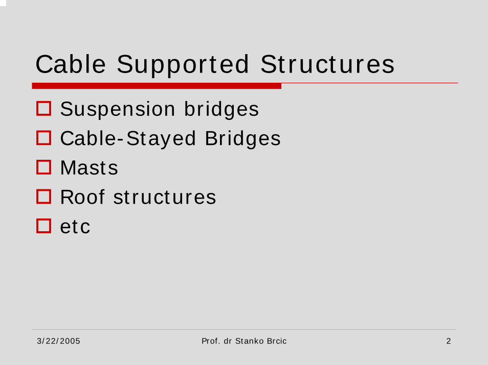
The maximum deflection of the cable:
If
then the max deflection is within the span of the cable.
0
0 max
( ) 0
( ) [cosh( ) 1]
Hy x x xq
Hy x yq
′ = ⇒ = = ⋅Φ
= = ⋅ Φ −
00 x l≤ ≤

3/22/2005 Prof. dr Stanko Brcic 13
Cable Analysis – dead load
Extreme values of support denivelation b in order to have are:00 x l≤ ≤
2 2
2max
2 2sinh ( ) sinh ( )
2| | sinh ( )
H Hb orq q
Hb bq
λ λ
λ
− ≤ ≤
≤ =
3/22/2005 Prof. dr Stanko Brcic 14
Cable Analysis – dead load

3/22/2005 Prof. dr Stanko Brcic 15
Cable Analysis – dead load
The cable with horizontal span: b = 0
0 max 1
2
( ) [cosh( ) cosh( )]
( ) sinh( )
, [cosh( ) 1]2 2
qlH
H qxy xq H
qxy xH
H H ql l Hx y fq q H q
λ
λ λ
λ
λ λ
Φ = =
= − −
′ = − −
= = ⋅ = = = −

3/22/2005 Prof. dr Stanko Brcic 16
Cable Analysis – dead load
For horizontal span b = 0:since,
one obtains the max deflection as
2
cosh( ) 12λλ ≅ +
2 2
max 2 8H qlyq H
λ= ⋅ =

3/22/2005 Prof. dr Stanko Brcic 17
Cable Analysis – dead load
The total length of the cable L:
Since
One obtains the length L as:
2
0 0
1x l l
x
dsL dx y dxdx
=
=
′= = +∫ ∫
2 2 21 1 sinh ( ) cosh ( )qx qxyH H
′+ = + −Φ = −Φ
2 sinh( )cosh( )HLq
λ λ= Φ −

3/22/2005 Prof. dr Stanko Brcic 18
Cable Analysis – dead load
For cable with horizontal span, the length L of the cable is:
02 sinh( )
bHLq
λ
λ
= ⇒ Φ =
=

3/22/2005 Prof. dr Stanko Brcic 19
Cable Analysis – dead load
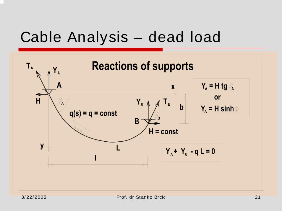
Reactions of supports at A and B:
Vertical component Ya is equal to(after transformation)
0( ) | ( ) |
A A B B
A x B x l
T H Y T H Ydy dyY H Y Hdx dx= =
= + = +
= ⋅ = − ⋅
sinh [ coth( )]2A AqY H Y L b λ= Φ ⇒ = +

3/22/2005 Prof. dr Stanko Brcic 20
Cable Analysis – dead load
Vertical component Yb is obtained from equilibrium condition:
For the cable with horizontal span:
0 [ coth( )]2A B BqY Y qL Y L b λ+ − = ⇒ = −
12A BY Y qL= =
3/22/2005 Prof. dr Stanko Brcic 21
Cable Analysis – dead load
3/22/2005 Prof. dr Stanko Brcic 22
Cable Analysis – dead load
PARABOLIC RELATIONSAssumption: The cable is relatively shallow, orThe gravitational loading is distributed along the horizontal projection of the cable

3/22/2005 Prof. dr Stanko Brcic 23
Cable Analysis – dead load

3/22/2005 Prof. dr Stanko Brcic 24
Cable Analysis – dead load

3/22/2005 Prof. dr Stanko Brcic 25
Cable Analysis – dead load
For deep cable (catenary) differential equation of equilibrium is
For shallow cable (parabolic relations)
21 0Hy q y′′ ′+ + =
1.0 0ds Hy qdx
′′≈ ⇒ + =
3/22/2005 Prof. dr Stanko Brcic 26
Cable Analysis – dead load
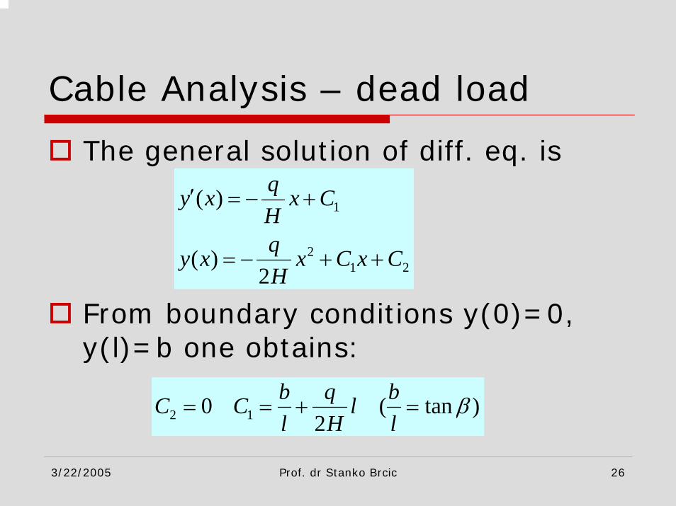
The general solution of diff. eq. is
From boundary conditions y(0)=0, y(l)=b one obtains:
1
21 2
( )
( )2
qy x x CHqy x x C x CH
′ = − +
= − + +
2 10 ( tan )2
b q bC C ll H l
β= = + =

3/22/2005 Prof. dr Stanko Brcic 27
Cable Analysis – dead load
Therefore, the final solution is
The cable shape is parabola.Position of maximum deflection:
2
( ) ( 2 )2
( ) ( )2
q by x l xH l
q by x lx x xH l
′ = − +
= − +
0( ) 02l H by x x
q l′ = ⇒ = +

3/22/2005 Prof. dr Stanko Brcic 28
Cable Analysis – dead load
Therefore, the max deflection is:
Extreme support denivelation to have max deflection within the cable span:
2 2
0 max 2( )8 2 2ql b H by x yH q l
= = + +
2 2 2
max| |2 2 2ql ql qlb or b bH H H
− ≤ ≤ ≤ =

3/22/2005 Prof. dr Stanko Brcic 29
Cable Analysis – dead load
The length of the cable L:
It is obtained:
2 2 2
0
11 1 12
l
L y dx y y′ ′ ′= + + ≈ +∫
2 2
2
1 116 2 2
10 : 16 2
ql bL lH l
qlfor b L lH
⎡ ⎤⎛ ⎞ ⎛ ⎞≅ + +⎢ ⎥⎜ ⎟ ⎜ ⎟⎝ ⎠ ⎝ ⎠⎢ ⎥⎣ ⎦
⎡ ⎤⎛ ⎞= ≅ +⎢ ⎥⎜ ⎟⎝ ⎠⎢ ⎥⎣ ⎦

3/22/2005 Prof. dr Stanko Brcic 30
Cable Analysis – dead load
Vertical components of support reactions are:
It is obtained:
For horizontal span (b = 0):
0| |A x B x lY Hy Y Hy= =′ ′= = −
2 2A Bql b ql bY H Y H
l l= + = −
2A BqlY Y= =

3/22/2005 Prof. dr Stanko Brcic 31
Cable Analysis – dead load
Hyperbolic or Parabolic relations:the solution depends on H, i.e. on the unknown horizontal cable tensionStatically undetermined problemInitial assumption of H or max cable tension orInitial assumption of the total cable length

3/22/2005 Prof. dr Stanko Brcic 32
Elastic Cables – The Cable Equation
Cable is ideally elastic body (material line) with equivalent
- Modulus of elasticity- Coefficient of thermal expansionTwo loading conditions are considered: initial loading (self-weight) and some additional loading (live load)

3/22/2005 Prof. dr Stanko Brcic 33
Elastic Cables – The Cable Equation
For initial loading the cable element is given as:Due to some additional loading the cable moves to the new equilibrium configuration (displacement components u, v). The cable element in the new configuration is
2 2 2ds dx dy= +
2 2 2( ) ( )ds dx du dy dv′ = + + +

3/22/2005 Prof. dr Stanko Brcic 34
Elastic Cables – The Cable Equation
Dilatation of a point at the cable element is given as:
If neglecting the small quantities of the 2nd order:
21 ( )2
ds ds dx du dy dv dvds ds ds ds ds ds
ε′ −
= = + +
ds ds dx du dy dvds ds ds ds ds
ε′ −
= = +

3/22/2005 Prof. dr Stanko Brcic 35
Elastic Cables – The Cable Equation
Increment of cable tension due to additional load is denoted as τ. The corresponding horizontal component of that increment in tension is h:
cosdx dsh hds dx
τ τ ϕ τ= = ⇒ =

3/22/2005 Prof. dr Stanko Brcic 36
Elastic Cables – The Cable Equation
Therefore, the Hooke’s Law is
Consequently, it may be obtained:
t tEAτε α= + ∆
21 ( )2t
dsh dx du dy dv dvdx tEA ds ds ds ds ds
α+ ∆ = + +

3/22/2005 Prof. dr Stanko Brcic 37
Elastic Cables – The Cable Equation
After multiplying with the cable equation in differential form is obtained
If neglecting the 2nd order terms, then:
2dsdx
⎛ ⎞⎜ ⎟⎝ ⎠
3
2 2( ) 1( ) ( )
2t
dsh ds du dy dv dvdx tEA dx dx dx dx dx
α+ ∆ = + +
3
2( )
( )t
dsh ds du dy dvdx tEA dx dx dx dx
α+ ∆ = +

3/22/2005 Prof. dr Stanko Brcic 38
Elastic Cables – The Cable Equation
Integrating over the span of the cable, one obtains the Integral form of the Cable equation:
Or in the form
2
0 0
1( ) (0) ( )2
l le
t thL dy dv dvtL u l u dx dxAE dx dx dx
α+ ∆ = − + +∫ ∫
0
( ) (0)l
et t
hL dy dvtL u l u dxAE dx dx
α+ ∆ = − + ∫
3/22/2005 Prof. dr Stanko Brcic 39
Elastic Cables – The Cable Equation
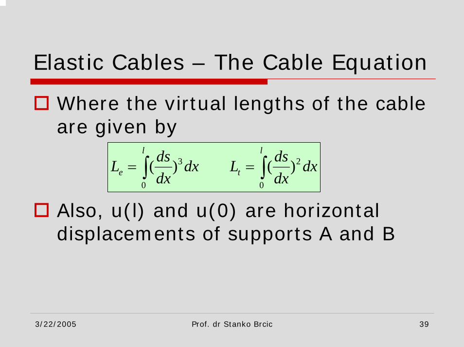
Where the virtual lengths of the cable are given by
Also, u(l) and u(0) are horizontal displacements of supports A and B
3 2
0 0
( ) ( )l l
e tds dsL dx L dxdx dx
= =∫ ∫

3/22/2005 Prof. dr Stanko Brcic 40
Elastic Cables – The Cable Equation
For Hyperbolic relations the virtual lengths may be obtained as:
which may be transformed into
3 2
0 0
cosh ( ) cosh ( )l l
e tqx qxL dx L dxH H
= −Φ = −Φ∫ ∫
3sinh(3 )cosh 3( ) sinh( )cosh( )6 2
sinh(2 )cosh 2( )2 2
e
t
H HLq q
H lLq
λ λ λ λ
λ λ
= Φ − + Φ −
= Φ − +

3/22/2005 Prof. dr Stanko Brcic 41
Elastic Cables – The Cable Equation
For the cable with horizontal span (b = 0):
1[ sinh(3 ) 3sinh( )]2 3
sinh(2 ) ,2 2 2
e
t
HLq
H l qlLq H
λ λ
λ λ λ
= +
= + = Φ =

3/22/2005 Prof. dr Stanko Brcic 42
Elastic Cables – The Cable Equation
For the Parabolic relations, the virtual cable lengths are obtained as
After integration, it is obtained
2 3/ 2 2
0 0
(1 ) (1 )l l
e tL y dx L y dx′ ′= + = +∫ ∫
2 4 22 2
2 22
96 3 11 8 1 8 tan tan5 2 4
161 tan , tan ,3 8 4
e
t
f f fL ll l l
f ql b fL l fl H l l
β β
λβ β
⎧ ⎫⎡ ⎤⎪ ⎪⎛ ⎞ ⎛ ⎞ ⎛ ⎞≈ + + + + +⎢ ⎥⎨ ⎬⎜ ⎟ ⎜ ⎟ ⎜ ⎟⎝ ⎠ ⎝ ⎠ ⎝ ⎠⎢ ⎥⎪ ⎪⎣ ⎦⎩ ⎭
⎡ ⎤⎛ ⎞≈ + + = = =⎢ ⎥⎜ ⎟⎝ ⎠⎢ ⎥⎣ ⎦

3/22/2005 Prof. dr Stanko Brcic 43
Elastic Cables – The Cable Equation
By the partial integration one obtains
For the boundary conditions v(0) = 0 and v(l) = 0, and for the parabolic relations, since
2
0 20 0
|l l
ldy dv dy d ydx v vdxdx dx dx dx
= −∫ ∫
2
2
d y q constdx H
= − =
3/22/2005 Prof. dr Stanko Brcic 44
Elastic Cables – The Cable Equation
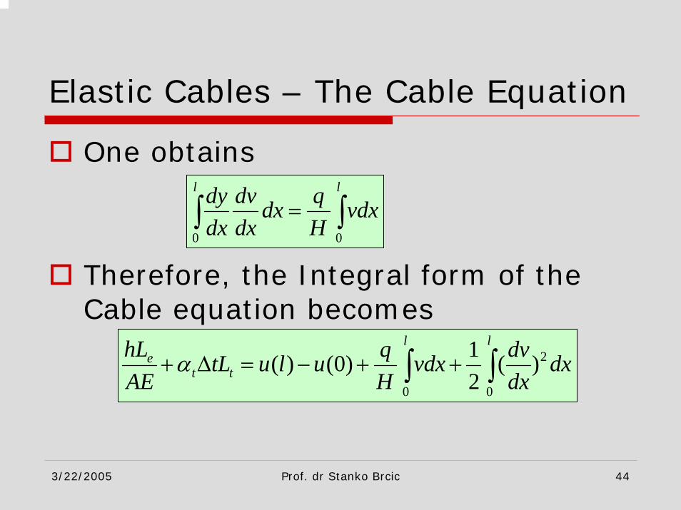
One obtains
Therefore, the Integral form of the Cable equation becomes
0 0
l ldy dv qdx vdxdx dx H
=∫ ∫
2
0 0
1( ) (0) ( )2
l le
t thL q dvtL u l u vdx dxAE H dx
α+ ∆ = − + +∫ ∫

3/22/2005 Prof. dr Stanko Brcic 45
Elastic Cables – The Cable Equation
or, if neglecting the small terms of the 2nd order,
If the supports are fixed, thenu(l) = u(0) = 0
0
( ) (0)l
et t
hL qtL u l u vdxAE H
α+ ∆ = − + ∫
3/22/2005 Prof. dr Stanko Brcic 46
Live Load and Temperature Effects upon the Cable (Parabolic relations)
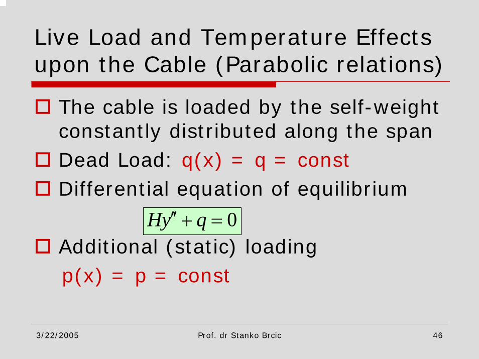
The cable is loaded by the self-weight constantly distributed along the spanDead Load: q(x) = q = constDifferential equation of equilibrium
Additional (static) loadingp(x) = p = const
0Hy q′′ + =

3/22/2005 Prof. dr Stanko Brcic 47
Live Load and Temperature Effects upon the Cable (Parabolic relations)

3/22/2005 Prof. dr Stanko Brcic 48
Live Load and Temperature Effects upon the Cable (Parabolic relations)
Due to additional load p, increment in horizontal component of cable tension is denoted as h, so differential equation of equilibrium is given as
Due to initial equilibrium equation ⇒( ) ( ) ( ) 0H h y v q p′′+ ⋅ + + + =
( ) ( )qH h v h p aH
′′+ − = −

3/22/2005 Prof. dr Stanko Brcic 49
Live Load and Temperature Effects upon the Cable (Parabolic relations)
It is possible to neglect the productas relatively small, so one obtains
Equation (a) or (b), together with the cable equation, say in the form
h v′′⋅
( )qHv h p bH
′′ − = −
0
( )l
et t
hL qtL vdx cAE H
α+ ∆ = ∫

3/22/2005 Prof. dr Stanko Brcic 50
Live Load and Temperature Effects upon the Cable (Parabolic relations)
define the problem of additional load (live load)Consider eqs. (b) and (c). From (b) ⇒
If v(0) = v(l) = 0, then
* 2
hq pv A constH H
′′ = = − =
2*
1( ) ( )2
v x A x lx= −

3/22/2005 Prof. dr Stanko Brcic 51
Live Load and Temperature Effects upon the Cable (Parabolic relations)
Therefore:
If this integral is introduced into the cable equation (c), one obtains the linear equation for unknown tension increment h
3*
0
1( )12
l
v x dx A l= −∫
3 2 3
2 3
1 112 12
et t
hL ql q ltL p hAE H H
α+ ∆ = −

3/22/2005 Prof. dr Stanko Brcic 52
Live Load and Temperature Effects upon the Cable (Parabolic relations)
With notation (catenary, or cable parameter)
horizontal tension increment h is obtained as
2 3
* 3e
q l AEH L
λ =
*
* *
1212 12
L tt
e
Lp AEh H tq L
λα
λ λ= ⋅ ⋅ − ∆ ⋅
+ +
3/22/2005 Prof. dr Stanko Brcic 53
Live Load and Temperature Effects upon the Cable (Parabolic relations)
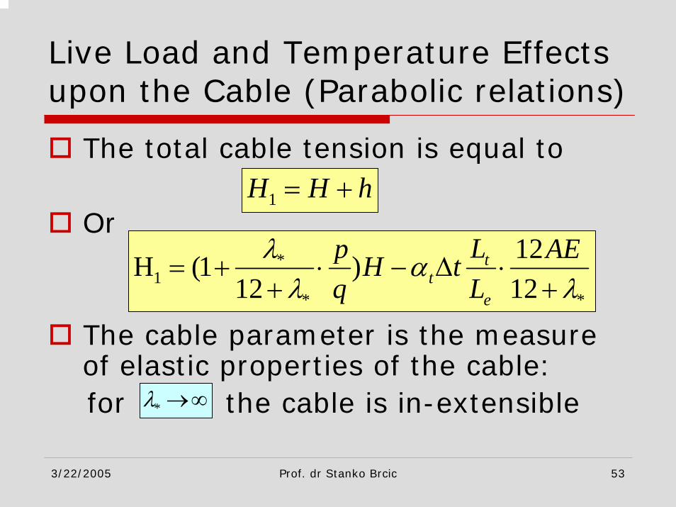
The total cable tension is equal to
Or
The cable parameter is the measure of elastic properties of the cable:for the cable is in-extensible
1H H h= +
*1
* *
12H (1 )12 12
tt
e
Lp AEH tq L
λ αλ λ
= + ⋅ − ∆ ⋅+ +
*λ →∞
3/22/2005 Prof. dr Stanko Brcic 54
Live Load and Temperature Effects upon the Cable (Parabolic relations)
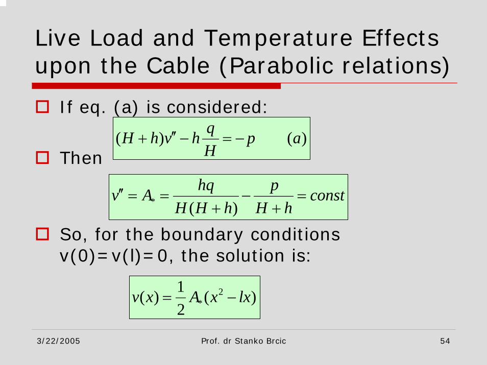
If eq. (a) is considered:
Then
So, for the boundary conditions v(0)=v(l)=0, the solution is:
( ) ( )qH h v h p aH
′′+ − = −
* ( )hq pv A const
H H h H h′′ = = − =
+ +
2*
1( ) ( )2
v x A x lx= −

3/22/2005 Prof. dr Stanko Brcic 55
Live Load and Temperature Effects upon the Cable (Parabolic relations)
The cable equation, for ∆t=0 and for u(0)=u(l)=0, is given as:
Therefore,
2
0 0
12
l lehL q vdx v dx
AE H′= +∫ ∫
3 2 2 3* *
0 0
1 112 12
l l
vdx A l v dx A l′= − =∫ ∫

3/22/2005 Prof. dr Stanko Brcic 56
Live Load and Temperature Effects upon the Cable (Parabolic relations)
With notation for non-dimensional increment of cable tension:
and the catenary (cable) parameter
hH
α =
2 3
* 3e
q l EAH L
λ =

3/22/2005 Prof. dr Stanko Brcic 57
Live Load and Temperature Effects upon the Cable (Parabolic relations)
the Cable equation may be written in the non-dimensional form of:
i.e. as the cubic equation in non-dimensional increment of cable tension h
3 2 2* * *(2 ) (1 ) [2( ) ( ) ]24 12 24
p pq q
λ λ λα α α+ + ⋅ + + ⋅ = +
3/22/2005 Prof. dr Stanko Brcic 58
Live Load and Temperature Effects upon the Cable (Parabolic relations)
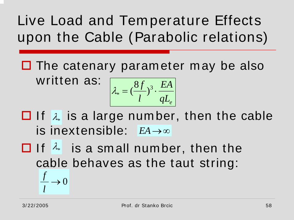
The catenary parameter may be also written as:
If is a large number, then the cable is inextensible: If is a small number, then the cable behaves as the taut string:
3*
8( )e
f EAl qL
λ = ⋅
*λEA→∞
*λ
0fl→

3/22/2005 Prof. dr Stanko Brcic 59
Live Load and Temperature Effects upon the Cable (Parabolic relations)
Obtaining solution of the cubic cable equation, tension increment is given. The final horizontal cable tension, due to additional load p, is given as:
Also, new deflection shape is given as1 (1 )H H h Hα= + = +
2*
1( ) ( )2
v x A x lx= −

3/22/2005 Prof. dr Stanko Brcic 60
Live Load and Temperature Effects upon the Cable (Parabolic relations)
Non-dimensional cable equation
represents the change in cable tension due to additional load.Non-linear dependence on additional load pNon-linearity is greater for smaller values of catenary parameter
3 2 2* * *(2 ) (1 ) [2( ) ( ) ]24 12 24
p pq q
λ λ λα α α+ + ⋅ + + ⋅ = +
*λ

3/22/2005 Prof. dr Stanko Brcic 61
Live Load and Temperature Effects upon the Cable (Parabolic relations)
For > 5000 non-linearity is relatively small
Limiting value of non-dimensional increment of cable tension is:
*λ
*
lim pqλ
α→∞
=

3/22/2005 Prof. dr Stanko Brcic 62
Live Load and Temperature Effects upon the Cable (Parabolic relations)
In the case of the cable equation where the second-order term is neglected, i.e.
and diff. equation of equilibrium (a), is used, the corresponding quadratic equation for increment of cable tension h is obtained
0
( )l
ehL q v x dxAE H
= ∫

3/22/2005 Prof. dr Stanko Brcic 63
Live Load and Temperature Effects upon the Cable (Parabolic relations)
In the case of simultaneous additionalload p and temperature load ∆t is considered, the cubic equation for incremental cable tension is obtained
3 2* *
2*
(2 ) (1 2 )24 12
[2( ) ( ) ]24
t tt t
e e
tt
e
L LAE AEt tL H L H
Lp p AEtq q L H
λ λα α α α α
λ α
+ + + ∆ ⋅ + + + ∆ ⋅ =
= + − ∆

3/22/2005 Prof. dr Stanko Brcic 64
Live Load and Temperature Effects upon the Cable (Parabolic relations)
New cable deflection after additional load p is given as:
New deflection may be transformed into the form similar to initial deflection due to dead load:
1( ) ( ) ( )y x y x v x= +
21 *( ) ( )
2q by x B lx x xH l
= ⋅ − +

3/22/2005 Prof. dr Stanko Brcic 65
Live Load and Temperature Effects upon the Cable (Parabolic relations)
where B is the non-dimensional deflection amplification:
Coefficient B is always > 1.0, sinceOnly for in-extensible cable
*
*
1 (1 ) 01
1 0
pB for hvq
pB for hvq
α
α
′′= ⋅ + ≠+
′′= + − =
pq
α>
* * 1.0EA Bλ →∞ ⇒ →∞ ⇒ →

3/22/2005 Prof. dr Stanko Brcic 66
Live Load and Temperature Effects upon the Cable (Parabolic relations)
Also, it may be concluded that the amplification of deflection B, due to additional loading, is greater for greater relative additional loading p/q, while the cable parameter λ is smaller.

3/22/2005 Prof. dr Stanko Brcic 67
Free Vibrations in the Cable Plane
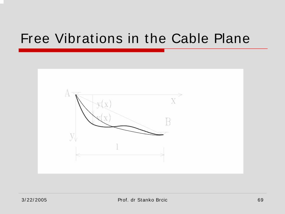
Cable is in the equilibrium configuration due to its self-weightParabolic approximation: dead load is uniform over the horizontal projection of cable: q(x) = q = constStatic equilibrium configuration: y(x)Free vibration in cable plane –dominant vertical motion v=v(x,t)

3/22/2005 Prof. dr Stanko Brcic 68
Free Vibrations in the Cable Plane
Free vibrations of a cable around its static equilibrium position.Position of a cable during free vibrations is given by:
1( , ) ( ) ( , )y x t y x v x t= +
3/22/2005 Prof. dr Stanko Brcic 69
Free Vibrations in the Cable Plane

3/22/2005 Prof. dr Stanko Brcic 70
Free Vibrations in the Cable Plane
According to D’Alembert’s Principle, the total load acting upon cable is:
(active and inertial forces), where m is cable mass per unit length:
1( , ) ( ) ( , )q x t q x mv x t= −
2
( )( ) 9.81q x mm x gg s
=

3/22/2005 Prof. dr Stanko Brcic 71
Free Vibrations in the Cable Plane
Horizontal component of cable tension is equal to
where H is due to dead load q, while h(t) is the cable tension increment due to inertial forces
1( ) ( ) ( )H t H h t H const= + =

3/22/2005 Prof. dr Stanko Brcic 72
Free Vibrations in the Cable Plane
Differential equation of “equilibrium”, according to D’Alembert’s Principle, is
Substituting, one obtains
or
1 1 1 0H y q′′+ =
( ) ( ) 0H h y v q mv′′+ ⋅ + + − =
0Hy Hv hy hv q mv′′ ′′ ′′ ′′+ + + + − =

3/22/2005 Prof. dr Stanko Brcic 73
Free Vibrations in the Cable Plane
Due to differential equation of static equilibrium: and neglecting the term (as the product of small increments), one obtains dif. equation of free vibrations of a cable:
0Hy q′′ + =
hv′′
0 ( )qmv Hv h aH
′′− + =
3/22/2005 Prof. dr Stanko Brcic 74
Free Vibrations in the Cable Plane
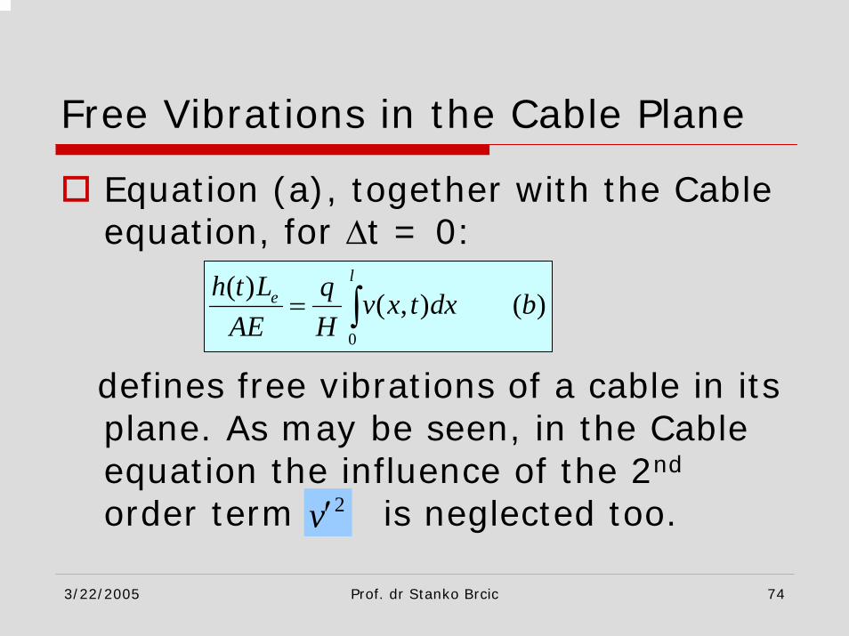
Equation (a), together with the Cable equation, for ∆t = 0:
defines free vibrations of a cable in its plane. As may be seen, in the Cable equation the influence of the 2nd
order term is neglected too.
0
( ) ( , ) ( )l
eh t L q v x t dx bAE H
= ∫
2v′

3/22/2005 Prof. dr Stanko Brcic 75
Free Vibrations in the Cable Plane
For harmonic free vibrations:
So, equations (a) and (b) become( , ) ( ) ( )i t i tv x t v x e h t h eω ω= ⋅ = ⋅
2
0
( .1)
( ) ( .2)l
e
qm v Hv h AH
hL q v x dx AAE H
ω ′′+ =
= ∫

3/22/2005 Prof. dr Stanko Brcic 76
Non-Symmetric Free Vibrations in the Cable Plane
Non-symmetric free vibrations are defined by non-symmetric function v(x,t) along the span of the cable:
In that case, it follows from (A.2) that also
0
( , ) 0l
v x t dx =∫
( ) 0h t =

3/22/2005 Prof. dr Stanko Brcic 77
Non-Symmetric Free Vibrations in the Cable Plane
Therefore, differential eq. of free non-symmetric vibrations is given as
The general solution is given by
where
2 0m v Hvω ′′+ =
1 2( ) sin( ) cos( )v x C kx C kx= +
mkH
ω=

3/22/2005 Prof. dr Stanko Brcic 78
Non-Symmetric Free Vibrations in the Cable Plane
Integration constants are determined from the boundary conditions:
The 2nd conditions is due to non-symmetry of free vibrations. Of course, the condition v(l) = 0 must be also fulfilled
(0) 0 ( ) 02lv v= =

3/22/2005 Prof. dr Stanko Brcic 79
Non-Symmetric Free Vibrations in the Cable Plane
From the boundary conditions one obtains:
The frequency equation is, therefore,
2 10 sin( ) 02klC C= =
sin( ) 0 , 1,2,3,2 2kl kl n nπ= ⇒ = = …
3/22/2005 Prof. dr Stanko Brcic 80
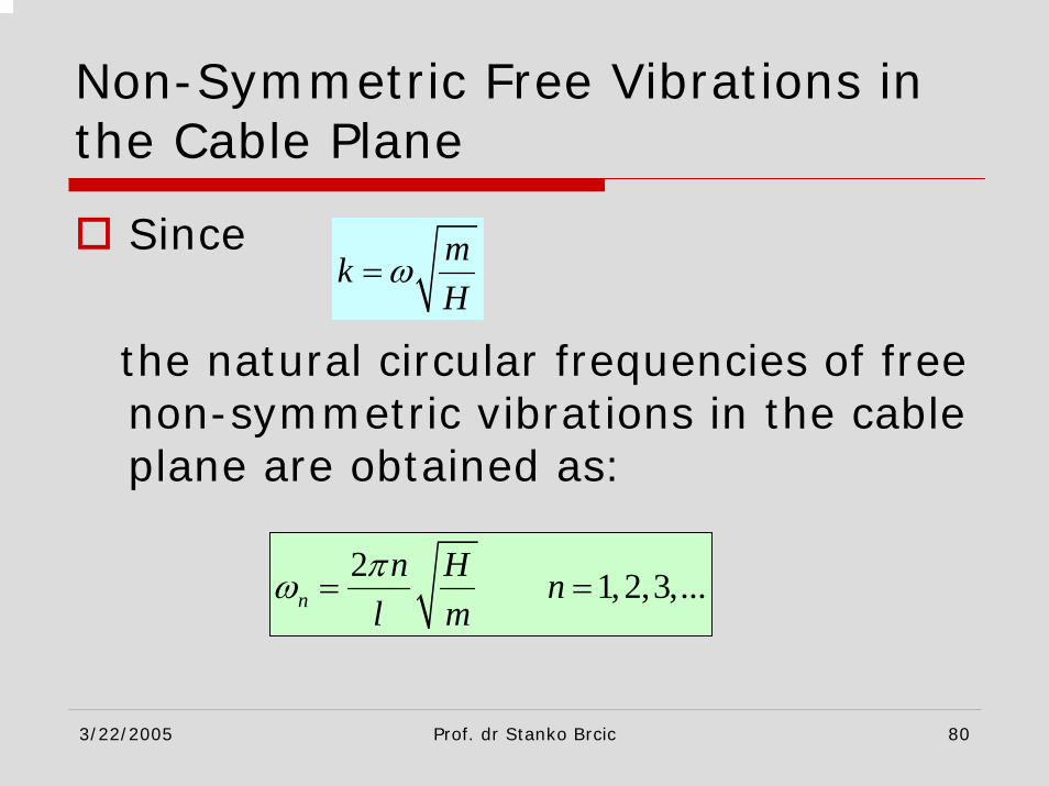
Non-Symmetric Free Vibrations in the Cable Plane
Since
the natural circular frequencies of free non-symmetric vibrations in the cable plane are obtained as:
mkH
ω=
2 1,2,3,...nn H n
l mπω = =

3/22/2005 Prof. dr Stanko Brcic 81
Non-Symmetric Free Vibrations in the Cable Plane
The corresponding natural shapes are given as:
It may also be seen that the solution satisfies the condition v(l) = 0
2( ) sin( ) 1,2,3,...n nnxv x C nlπ
= =
3/22/2005 Prof. dr Stanko Brcic 82
Symmetric Free Vibrations in the Cable Plane
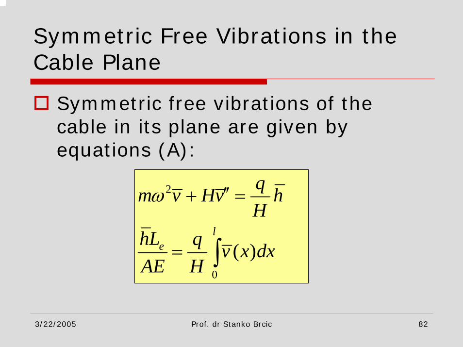
Symmetric free vibrations of the cable in its plane are given by equations (A):
2
0
( )l
e
qm v Hv hH
hL q v x dxAE H
ω ′′+ =
= ∫

3/22/2005 Prof. dr Stanko Brcic 83
Symmetric Free Vibrations in the Cable Plane
The general solution of differential equation is given as:
where the general solution of homogeneous equation is
while is any particular solution of non-homogeneous equation.
( ) ( ) ( )h pv x v x v x= +
1 2( ) sin( ) cos( )hv x C kx C kx= +
( )pv x

3/22/2005 Prof. dr Stanko Brcic 84
Symmetric Free Vibrations in the Cable Plane
The particular solution is
so the general solution is given as
2( )pqhv x
m Hω=
1 2 2( ) sin( ) cos( )hqhv x C kx C kx
m Hω= + +

3/22/2005 Prof. dr Stanko Brcic 85
Symmetric Free Vibrations in the Cable Plane
Integration constants are obtained from the boundary conditions:
It may be obtained:
(0) 0 ( ) 0v v l= =
2 12 2
(1 cos ),sin
qh qh klC Cm H m H klω ω
−= − = − ⋅

3/22/2005 Prof. dr Stanko Brcic 86
Symmetric Free Vibrations in the Cable Plane
Therefore, the general solution of diff. equation is obtained as:
This general solution is inserted into the integral of the 2nd equation (the cable equation).
2 2 2
(1 cos )( ) sin cossin
qh kl qh qhv x kx kxm H kl m H m Hω ω ω
−= − ⋅ ⋅ − ⋅ +

3/22/2005 Prof. dr Stanko Brcic 87
Symmetric Free Vibrations in the Cable Plane
It is obtained
Inserting this into the cable equation, and dividing by it is obtained
0 2
2 2 20
(1 cos )( ) sinsin
qh kl qh qhv x dx kl lm Hk kl m Hk m Hω ω ω
−= ⋅ − ⋅ + ⋅∫
0h ≠
2 2 2 2
3 2 2 2 2 2 2
(1 cos ) sin 0sin
eL q kl q qkl lAEl m H k kl m H k m Hω ω ω
−+ ⋅ + ⋅ − ⋅ =

3/22/2005 Prof. dr Stanko Brcic 88
Symmetric Free Vibrations in the Cable Plane
Since
the last equation may be transformed as
2 3 Hk km
ω =
2 2
3 3 3
(1 cos ) sin 0( ) sin
eL q kl kl klAEl H kl kl
⎡ ⎤−+ + − =⎢ ⎥
⎣ ⎦

3/22/2005 Prof. dr Stanko Brcic 89
Symmetric Free Vibrations in the Cable Plane
With notation
it may be obtained
from which
2 3
* 3e
m q l AEkl lH H L
ω ω λ= = =
*3 3
2(1 cos )1 0sin
eLAEl
λ ω ωω ω
⎧ ⎫−⎡ ⎤+ − =⎨ ⎬⎢ ⎥⎣ ⎦⎩ ⎭

3/22/2005 Prof. dr Stanko Brcic 90
Symmetric Free Vibrations in the Cable Plane
the frequency equation is obtained:
If the cable parameter is relatively large (cable tends to be in-extensible, which is NOT the case of cable-stayed bridges), then (c) becomes
3
*
4tan( ) ( ) ( ) ( )2 2 2
cω ω ωλ
= −
*λ
tan( ) ( )2 2
dω ω=
3/22/2005 Prof. dr Stanko Brcic 91
Symmetric Free Vibrations in the Cable Plane
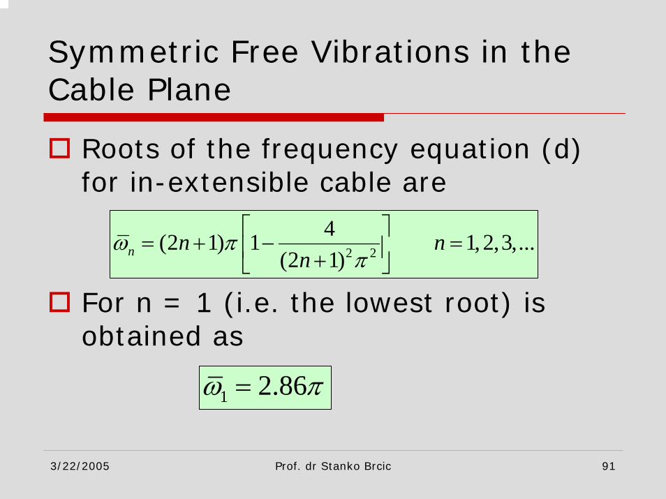
Roots of the frequency equation (d) for in-extensible cable are
For n = 1 (i.e. the lowest root) is obtained as
2 2
4(2 1) 1 1,2,3,...(2 1)n n n
nω π
π⎡ ⎤
= + − =⎢ ⎥+⎣ ⎦
1 2.86ω π=

3/22/2005 Prof. dr Stanko Brcic 92
Symmetric Free Vibrations in the Cable Plane
As may be seen, the roots of the frequency equation (c) depend on the cable parameter (which depends upon the loading, cross section, span, modulus of elasticity, cable tension).
*λ
3
*
4tan( ) ( ) ( ) ( )2 2 2
cω ω ωλ
= −
3/22/2005 Prof. dr Stanko Brcic 93
Symmetric Free Vibrations in the Cable Plane
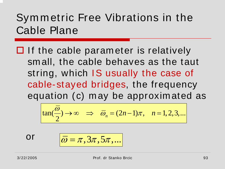
If the cable parameter is relatively small, the cable behaves as the taut string, which IS usually the case of cable-stayed bridges, the frequency equation (c) may be approximated as
or
tan( ) (2 1) , 1, 2,3,...2 n n nω ω π→∞ ⇒ = − =
,3 ,5 ,...ω π π π=

3/22/2005 Prof. dr Stanko Brcic 94
Symmetric Free Vibrations in the Cable Plane
Considering the notation for the natural circular frequencies of free symmetric vibrations in plane of the cable are:
where are solutions of the frequency equation
ω
1,2,3,...nn
H nl mωω = ⋅ =
nω

3/22/2005 Prof. dr Stanko Brcic 95
Symmetric Free Vibrations in the Cable Plane
Symmetric natural modes of free vibrations of the cable are given by
where is an arbitrary constant
2
1 cos( ) 1 sin cossin
n nn n n
n n
qhv x k x k xm H
ωω ω
⎡ ⎤−= − −⎢ ⎥
⎣ ⎦
nh

3/22/2005 Prof. dr Stanko Brcic 96
Orthogonality of Natural Modes –Non-Symmetric Vibrations
Two different natural modes of non-symmetric free vibrations are considered:
The first one is multiplied by and integrated over the span:
2
2
0 ( )
0 ( )p p p
q q q
m v Hv A
m v Hv p q
ω
ω
′′+ =
′′+ = ≠
2 0l l
p p q p qm v v dx H v v dxω ′′0 0
+ =∫ ∫
( )qv x

3/22/2005 Prof. dr Stanko Brcic 97
Orthogonality of Natural Modes –Non-Symmetric Vibrations
Partial integration of the 2nd integral:
Due to the boundary conditions, v(0)=v(l)=0, boundary terms are zero, while, due to the 2nd of eqs. (A),
00 0
[ ]l l
lp q p q p q p qv v dx v v v v v v dx′′ ′ ′ ′′= − +∫ ∫
2
0 0
l l
p q q p qH v v dx m v v dxω′′ = −∫ ∫

3/22/2005 Prof. dr Stanko Brcic 98
Orthogonality of Natural Modes –Non-Symmetric Vibrations
Consequently, it may be obtained
Since the natural frequencies are different, it follows that
i.e. natural modes are orthogonal.
2 2
0
( ) 0l
p q p qm v v dxω ω− ⋅ =∫
0
0l
p qv v dx =∫
3/22/2005 Prof. dr Stanko Brcic 99
Orthogonality of Natural Modes –Non-Symmetric Vibrations
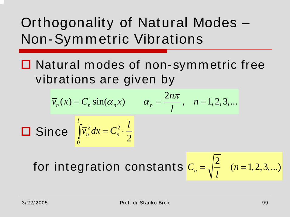
Natural modes of non-symmetric free vibrations are given by
Since
for integration constants
2( ) sin( ) , 1, 2,3,...n n n nnv x C x nlπα α= = =
2 2
0 2
l
n nlv dx C= ⋅∫
2 ( 1,2,3,...)nC nl
= =

3/22/2005 Prof. dr Stanko Brcic 100
Orthogonality of Natural Modes –Non-Symmetric Vibrations
natural modes of free non-symmetric vibrations are orthonormal:
0
01
2 2( ) sin , 1, 2,3,...
l
n m
n n n
n mv v dx
n m
nv x x nl l
πα α
≠⎧= ⎨ =⎩
= ⋅ = =
∫
3/22/2005 Prof. dr Stanko Brcic 101
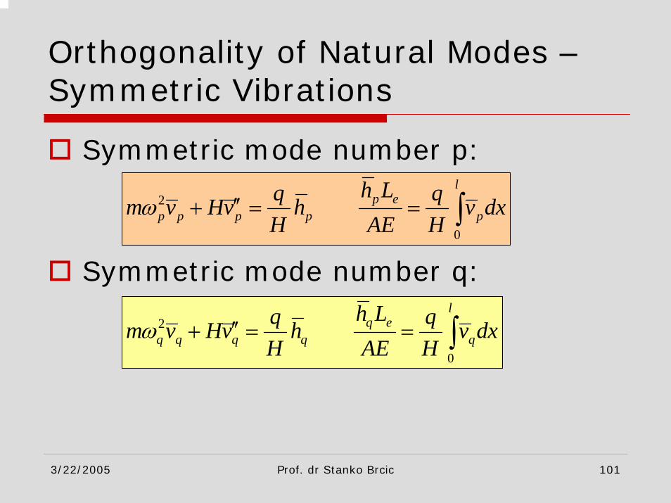
Orthogonality of Natural Modes –Symmetric Vibrations
Symmetric mode number p:
Symmetric mode number q:
2
0
lp e
p p p p p
h Lq qm v Hv h v dxH AE H
ω ′′+ = = ∫
2
0
lq e
q q q q q
h Lq qm v Hv h v dxH AE H
ω ′′+ = = ∫
3/22/2005 Prof. dr Stanko Brcic 102
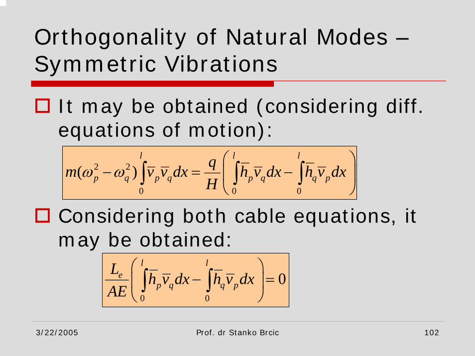
Orthogonality of Natural Modes –Symmetric Vibrations
It may be obtained (considering diff. equations of motion):
Considering both cable equations, it may be obtained:
2 2
0 0 0
( )l l l
p q p q p q q pqm v v dx h v dx h v dxH
ω ω⎛ ⎞
− = −⎜ ⎟⎝ ⎠
∫ ∫ ∫
0 0
0l l
ep q q p
L h v dx h v dxAE
⎛ ⎞− =⎜ ⎟
⎝ ⎠∫ ∫
3/22/2005 Prof. dr Stanko Brcic 103
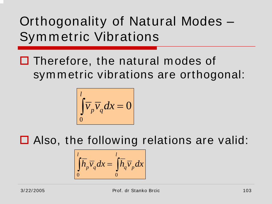
Orthogonality of Natural Modes –Symmetric Vibrations
Therefore, the natural modes of symmetric vibrations are orthogonal:
Also, the following relations are valid:
0
0l
p qv v dx =∫
0 0
l l
p q q ph v dx h v dx=∫ ∫
3/22/2005 Prof. dr Stanko Brcic 104
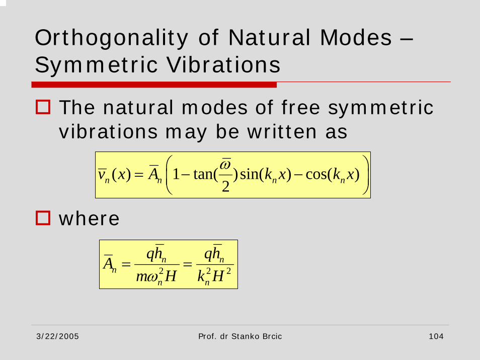
Orthogonality of Natural Modes –Symmetric Vibrations
The natural modes of free symmetric vibrations may be written as
where
( ) 1 tan( )sin( ) cos( )2n n n nv x A k x k xω⎛ ⎞= − −⎜ ⎟
⎝ ⎠
2 2 2n n
nn n
qh qhAm H k Hω
= =
3/22/2005 Prof. dr Stanko Brcic 105
Orthogonality of Natural Modes –Symmetric Vibrations
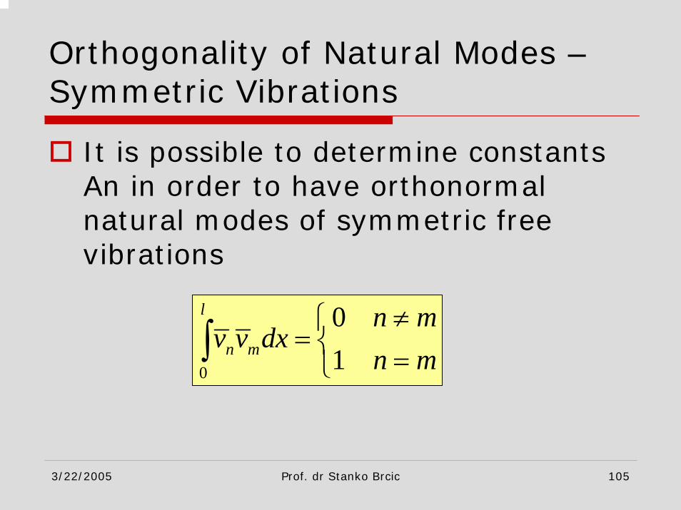
It is possible to determine constants An in order to have orthonormalnatural modes of symmetric free vibrations
0
01
l
n m
n mv v dx
n m≠⎧
= ⎨ =⎩∫

3/22/2005 Prof. dr Stanko Brcic 106
Free Vibrations of Cables outside of the Cable Plane
Free vibrations without the change of cable shape – PENDULUM ModeShallow cable with horizontal slope (b=0)Dead load of the cable q(x) = mg = constParabolic relations

3/22/2005 Prof. dr Stanko Brcic 107
Free Vibrations of Cables outside of the Cable Plane – Pendulum Mode

3/22/2005 Prof. dr Stanko Brcic 108
Free Vibrations of Cables outside of the Cable Plane – Pendulum Mode
In the pendulum mode the cable retains its shape and the plane of cable rotates about horizontal axis x.Generalized coordinate: angle ϕbetween x-y (initial vertical) plane and current cable plane during pendulum motion.

3/22/2005 Prof. dr Stanko Brcic 109
Free Vibrations of Cables outside of the Cable Plane – Pendulum Mode
Element of the cable arc:- length ds- mass dm = m ds = q/g ds (g=9.81)
Differential equation of motion of the cable element:
2 2
sinx
x
J M dJ qds
dJ dm mds
ε ϕ η ϕ
η η
= ⇒ = − ⋅
= =
3/22/2005 Prof. dr Stanko Brcic 110
Free Vibrations of Cables outside of the Cable Plane – Pendulum Mode
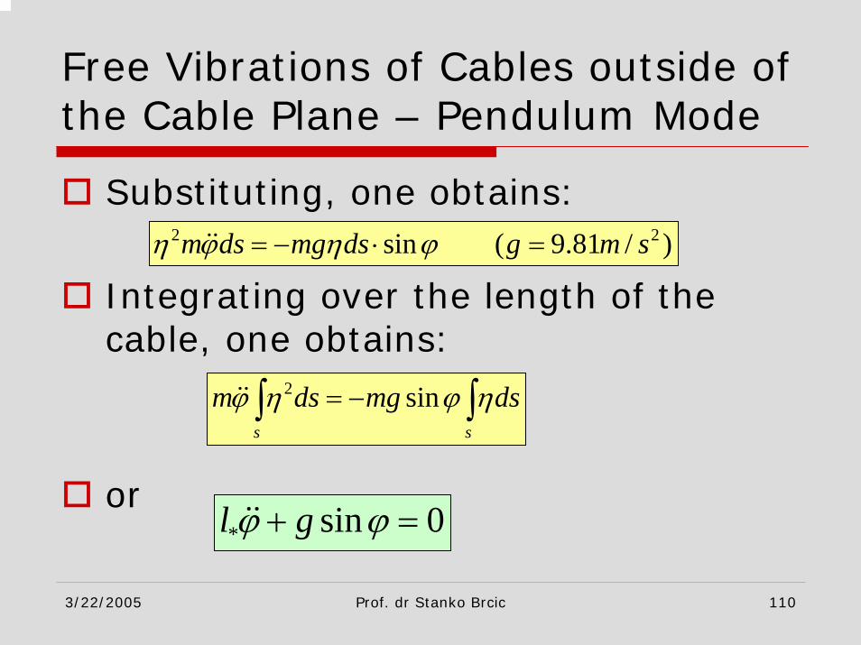
Substituting, one obtains:
Integrating over the length of the cable, one obtains:
or
2 2sin ( 9.81 / )m ds mg ds g m sη ϕ η ϕ= − ⋅ =
2 sins s
m ds mg dsϕ η ϕ η= −∫ ∫
* sin 0l gϕ ϕ+ =
3/22/2005 Prof. dr Stanko Brcic 111
Free Vibrations of Cables outside of the Cable Plane – Pendulum Mode
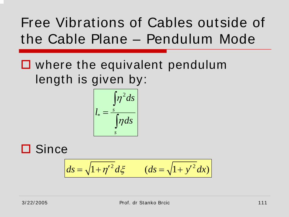
where the equivalent pendulum length is given by:
Since
2
*s
s
dsl
ds
η
η=∫
∫
2 21 ( 1 )ds d ds y dxη ξ′ ′= + = +

3/22/2005 Prof. dr Stanko Brcic 112
Free Vibrations of Cables outside of the Cable Plane – Pendulum Mode
so, the equivalent pendulum length is given as
With approximation:
2 2
0*
2
0
1
1
l
l
dl
d
η η ξ
η η ξ
′+=
′+
∫
∫
2 211 12
y y′ ′+ ≈ +

3/22/2005 Prof. dr Stanko Brcic 113
Free Vibrations of Cables outside of the Cable Plane – Pendulum Mode
And also, for parabolic relations and horizontal span:
It may be obtained
22 2
2
4( ) ( )2 8q f qll l fH l H
η ξ ξ ξ ξ= − = − =
2
*2
81 ( )4 7 0.8085 1 ( )5
fll f ffl
+= ⋅ ≈ ⋅
+

3/22/2005 Prof. dr Stanko Brcic 114
Free Vibrations of Cables outside of the Cable Plane – Pendulum Mode
Therefore, the equivalent pendulum length is about 80% of max cable deflectionFor relatively small angles of inclination ϕ: so, differential equation of motion becomes
sinϕ ϕ≈
2
*
0 gl
ϕ ω ϕ ω+ = =

3/22/2005 Prof. dr Stanko Brcic 115
Free Vibrations of Cables outside of the Cable Plane – Pendulum Mode
and represents the pendulum mode oscillation of the cable about horizontal axis in direction of span.For initial conditionsthe solution is given as
0 0(0) , (0)ϕ ϕ ϕ ϕ= =
00( ) cos sint t tϕϕ ϕ ω ω
ω= +

3/22/2005 Prof. dr Stanko Brcic 116
Free Vibrations of Cables outside of the Cable Plane – Pendulum Mode
If the angle ϕ is not small enough (but it is still small!), then one may assume approximation
Differential equation of motion is
31sin6
ϕ ϕ ϕ≈ −
2 2 2
*
1(1 ) 06
gl
ϕ ω ϕ ϕ ω+ − = =
3/22/2005 Prof. dr Stanko Brcic 117
Free Vibrations of Cables outside of the Cable Plane – Pendulum Mode
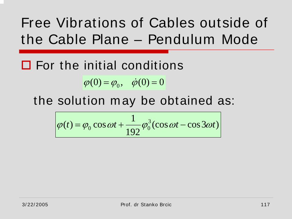
For the initial conditions
the solution may be obtained as:0(0) , (0) 0ϕ ϕ ϕ= =
30 0
1( ) cos (cos cos3 )192
t t t tϕ ϕ ω ϕ ω ω= + −
3/22/2005 Prof. dr Stanko Brcic 118
![Kinematics and Statics Including Cable Sag for Large Cable ... · Early View H. comparing the straight‐line cables assumption vs. a cable‐sag model. dit Sandretto et al. [14]](https://static.fdocument.org/doc/165x107/606f6dd64749a00bcf75834a/kinematics-and-statics-including-cable-sag-for-large-cable-early-view-h-comparing.jpg)