Quantitative stochastic homogenization and large-scale regularity
Regularity Structures
Martin Hairer
University of Warwick
Seoul, August 14, 2014
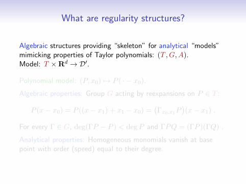
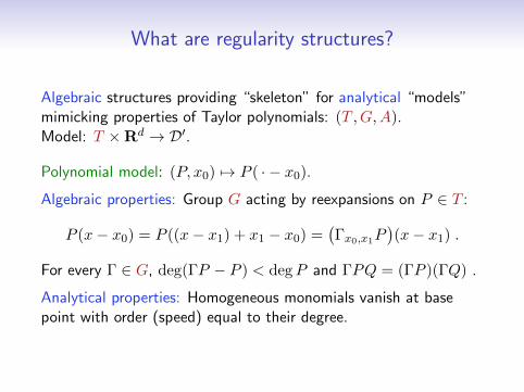
What are regularity structures?
Algebraic structures providing “skeleton” for analytical “models”mimicking properties of Taylor polynomials: (T ,G,A).Model: T ×Rd → D′.
Polynomial model: (P, x0) 7→ P ( · − x0).
Algebraic properties: Group G acting by reexpansions on P ∈ T :
P (x− x0) = P ((x− x1) + x1 − x0) =(Γx0,x1P
)(x− x1) .
For every Γ ∈ G, deg(ΓP − P ) < degP and ΓPQ = (ΓP )(ΓQ) .
Analytical properties: Homogeneous monomials vanish at basepoint with order (speed) equal to their degree.
Another example
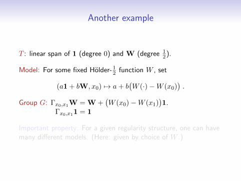
T : linear span of 1 (degree 0) and W (degree 12).
Model: For some fixed Holder-12 function W , set
(a1 + bW, x0) 7→ a+ b(W (·)−W (x0)
).
Group G: Γx0,x1W = W +(W (x0)−W (x1)
)1.
Γx0,x11 = 1
Important property: For a given regularity structure, one can havemany different models. (Here: given by choice of W .)
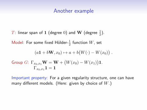
Another example
T : linear span of 1 (degree 0) and W (degree 12).
Model: For some fixed Holder-12 function W , set
(a1 + bW, x0) 7→ a+ b(W (·)−W (x0)
).
Group G: Γx0,x1W = W +(W (x0)−W (x1)
)1.
Γx0,x11 = 1
Important property: For a given regularity structure, one can havemany different models. (Here: given by choice of W .)
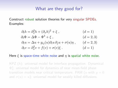
What are they good for?
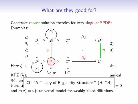
Construct robust solution theories for very singular SPDEs.Examples:
∂th = ∂2xh+ (∂xh)2 + ξ , (d = 1)
∂tΦ = ∆Φ− Φ3 + ξ , (d = 2, 3)
∂tu = ∆u+ gij(u)∂iu ∂ju+ σ(u)η , (d = 2, 3)
∂tv = ∂2xv + f(v) + σ(v)ξ . (d = 1)
Here ξ is space-time white noise and η is spatial white noise.
KPZ (h): universal model for interface propagation. DynamicalΦ43: universal model for dynamics of near mean-field phase
transition models near critical temperature. PAM (u with g = 0and σ(u) = u): universal model for weakly killed diffusions.
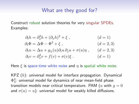
What are they good for?
Construct robust solution theories for very singular SPDEs.Examples:
∂th = ∂2xh+ (∂xh)2 + ξ , (d = 1)
∂tΦ = ∆Φ− Φ3 + ξ , (d = 2, 3)
∂tu = ∆u+ gij(u)∂iu ∂ju+ σ(u)η , (d = 2, 3)
∂tv = ∂2xv + f(v) + σ(v)ξ . (d = 1)
Here ξ is space-time white noise and η is spatial white noise.
KPZ (h): universal model for interface propagation. DynamicalΦ43: universal model for dynamics of near mean-field phase
transition models near critical temperature. PAM (u with g = 0and σ(u) = u): universal model for weakly killed diffusions.
F M
R
×× Cα Dγ
·
F
R
× ?
Noise
∈
× Cα
I.C.∈
Cα
RΨ
SA
SC
Cf. “A Theory of Regularity Structures” (H. ’14)
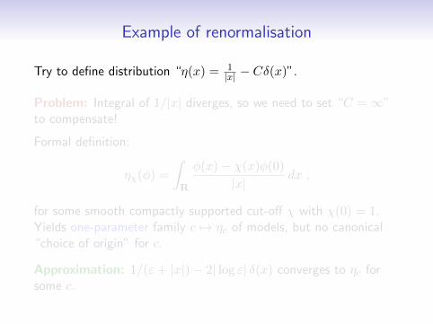
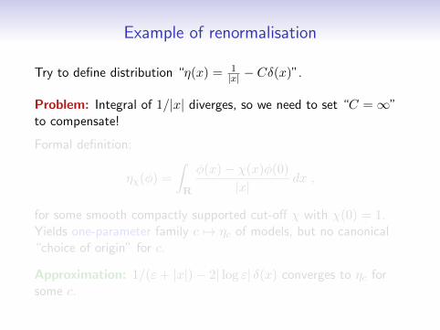
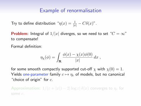
Example of renormalisation
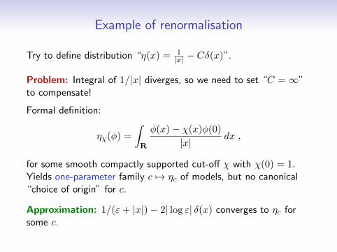
Try to define distribution “η(x) = 1|x| − Cδ(x)”.
Problem: Integral of 1/|x| diverges, so we need to set “C =∞”to compensate!
Formal definition:
ηχ(φ) =
∫R
φ(x)− χ(x)φ(0)
|x|dx ,
for some smooth compactly supported cut-off χ with χ(0) = 1.Yields one-parameter family c 7→ ηc of models, but no canonical“choice of origin” for c.
Approximation: 1/(ε+ |x|)− 2| log ε| δ(x) converges to ηc forsome c.
Example of renormalisation
Try to define distribution “η(x) = 1|x| − Cδ(x)”.
Problem: Integral of 1/|x| diverges, so we need to set “C =∞”to compensate!
Formal definition:
ηχ(φ) =
∫R
φ(x)− χ(x)φ(0)
|x|dx ,
for some smooth compactly supported cut-off χ with χ(0) = 1.Yields one-parameter family c 7→ ηc of models, but no canonical“choice of origin” for c.
Approximation: 1/(ε+ |x|)− 2| log ε| δ(x) converges to ηc forsome c.
Previous notions of solution
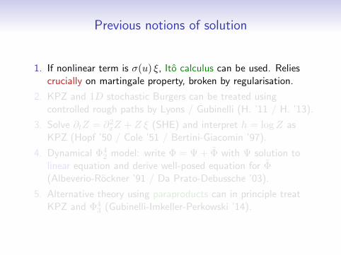
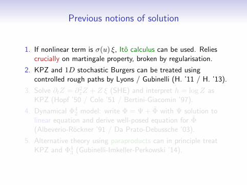
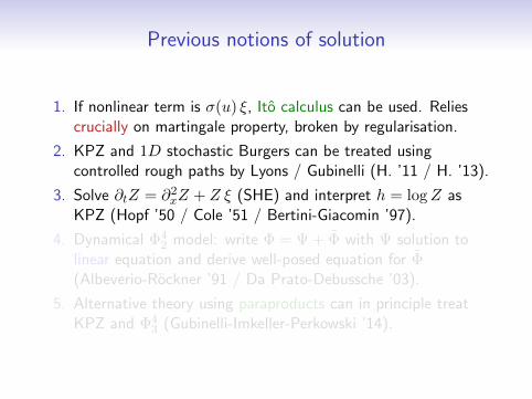
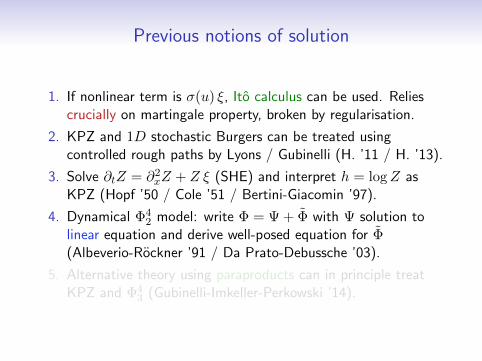
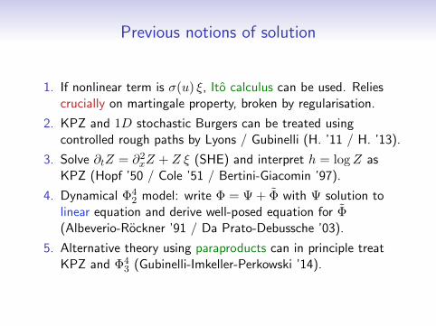
1. If nonlinear term is σ(u) ξ, Ito calculus can be used. Reliescrucially on martingale property, broken by regularisation.
2. KPZ and 1D stochastic Burgers can be treated usingcontrolled rough paths by Lyons / Gubinelli (H. ’11 / H. ’13).
3. Solve ∂tZ = ∂2xZ + Z ξ (SHE) and interpret h = logZ asKPZ (Hopf ’50 / Cole ’51 / Bertini-Giacomin ’97).
4. Dynamical Φ42 model: write Φ = Ψ + Φ with Ψ solution to
linear equation and derive well-posed equation for Φ(Albeverio-Rockner ’91 / Da Prato-Debussche ’03).
5. Alternative theory using paraproducts can in principle treatKPZ and Φ4
3 (Gubinelli-Imkeller-Perkowski ’14).
Previous notions of solution
1. If nonlinear term is σ(u) ξ, Ito calculus can be used. Reliescrucially on martingale property, broken by regularisation.
2. KPZ and 1D stochastic Burgers can be treated usingcontrolled rough paths by Lyons / Gubinelli (H. ’11 / H. ’13).
3. Solve ∂tZ = ∂2xZ + Z ξ (SHE) and interpret h = logZ asKPZ (Hopf ’50 / Cole ’51 / Bertini-Giacomin ’97).
4. Dynamical Φ42 model: write Φ = Ψ + Φ with Ψ solution to
linear equation and derive well-posed equation for Φ(Albeverio-Rockner ’91 / Da Prato-Debussche ’03).
5. Alternative theory using paraproducts can in principle treatKPZ and Φ4
3 (Gubinelli-Imkeller-Perkowski ’14).
Universality
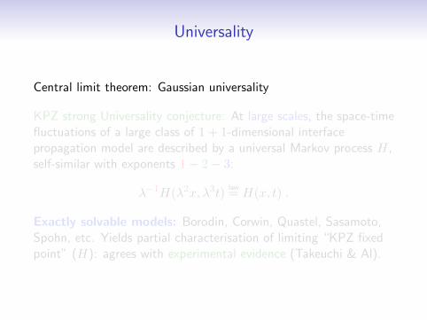
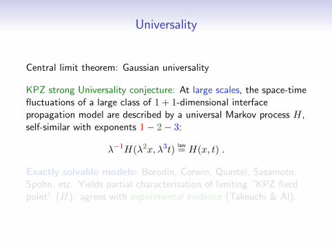
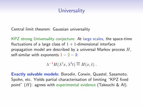
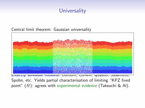
Central limit theorem: Gaussian universality
KPZ strong Universality conjecture: At large scales, the space-timefluctuations of a large class of 1 + 1-dimensional interfacepropagation model are described by a universal Markov process H,self-similar with exponents 1− 2− 3:
λ−1H(λ2x, λ3t)law= H(x, t) .
Exactly solvable models: Borodin, Corwin, Quastel, Sasamoto,Spohn, etc. Yields partial characterisation of limiting “KPZ fixedpoint” (H): agrees with experimental evidence (Takeuchi & Al).
Universality
Central limit theorem: Gaussian universality
KPZ strong Universality conjecture: At large scales, the space-timefluctuations of a large class of 1 + 1-dimensional interfacepropagation model are described by a universal Markov process H,self-similar with exponents 1− 2− 3:
λ−1H(λ2x, λ3t)law= H(x, t) .
Exactly solvable models: Borodin, Corwin, Quastel, Sasamoto,Spohn, etc. Yields partial characterisation of limiting “KPZ fixedpoint” (H): agrees with experimental evidence (Takeuchi & Al).
Heuristic picture
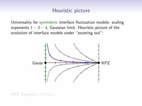
Universality for symmetric interface fluctuation models: scalingexponents 1− 2− 4, Gaussian limit. Heuristic picture of theevolution of interface models under “zooming out”:
Gauss KPZ
KPZ equation: red line.
Heuristic picture
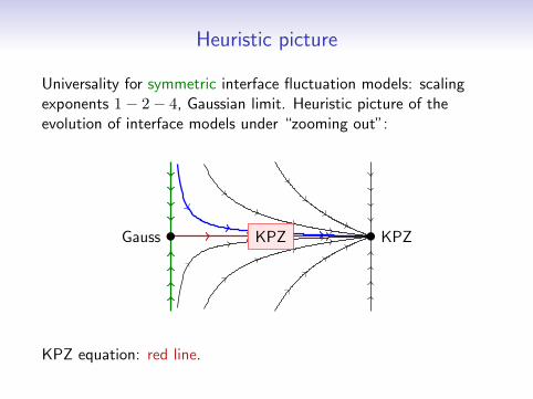
Universality for symmetric interface fluctuation models: scalingexponents 1− 2− 4, Gaussian limit. Heuristic picture of theevolution of interface models under “zooming out”:
Gauss KPZKPZ
KPZ equation: red line.
Weak Universality conjecture
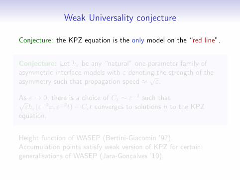
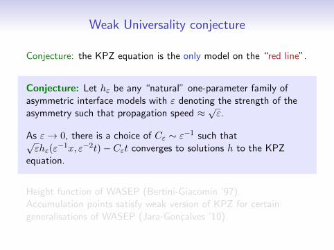
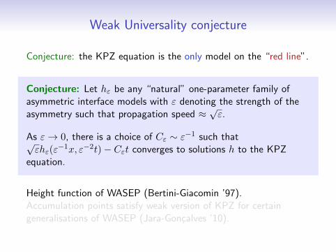
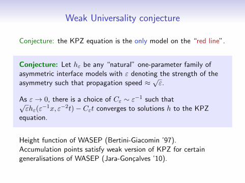
Conjecture: the KPZ equation is the only model on the “red line”.
Conjecture: Let hε be any “natural” one-parameter family ofasymmetric interface models with ε denoting the strength of theasymmetry such that propagation speed ≈
√ε.
As ε→ 0, there is a choice of Cε ∼ ε−1 such that√εhε(ε
−1x, ε−2t)− Cεt converges to solutions h to the KPZequation.
Height function of WASEP (Bertini-Giacomin ’97).Accumulation points satisfy weak version of KPZ for certaingeneralisations of WASEP (Jara-Goncalves ’10).
Weak Universality conjecture
Conjecture: the KPZ equation is the only model on the “red line”.
Conjecture: Let hε be any “natural” one-parameter family ofasymmetric interface models with ε denoting the strength of theasymmetry such that propagation speed ≈
√ε.
As ε→ 0, there is a choice of Cε ∼ ε−1 such that√εhε(ε
−1x, ε−2t)− Cεt converges to solutions h to the KPZequation.
Height function of WASEP (Bertini-Giacomin ’97).Accumulation points satisfy weak version of KPZ for certaingeneralisations of WASEP (Jara-Goncalves ’10).
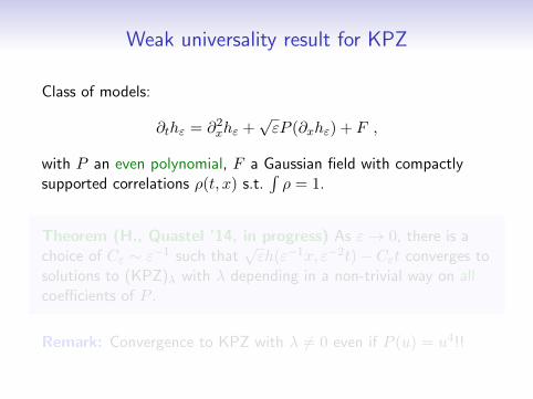
Weak universality result for KPZ
Class of models:
∂thε = ∂2xhε +√εP (∂xhε) + F ,
with P an even polynomial, F a Gaussian field with compactlysupported correlations ρ(t, x) s.t.
∫ρ = 1.
Theorem (H., Quastel ’14, in progress) As ε→ 0, there is achoice of Cε ∼ ε−1 such that
√εh(ε−1x, ε−2t)− Cεt converges to
solutions to (KPZ)λ with λ depending in a non-trivial way on allcoefficients of P .
Remark: Convergence to KPZ with λ 6= 0 even if P (u) = u4!!
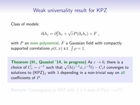
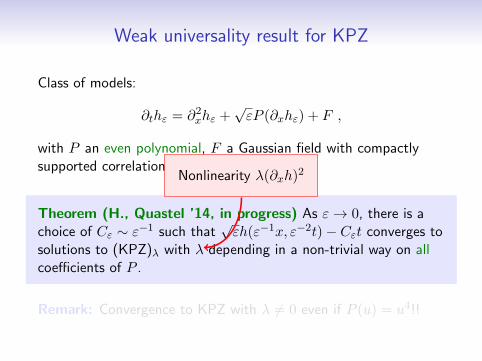
Weak universality result for KPZ
Class of models:
∂thε = ∂2xhε +√εP (∂xhε) + F ,
with P an even polynomial, F a Gaussian field with compactlysupported correlations ρ(t, x) s.t.
∫ρ = 1.
Theorem (H., Quastel ’14, in progress) As ε→ 0, there is achoice of Cε ∼ ε−1 such that
√εh(ε−1x, ε−2t)− Cεt converges to
solutions to (KPZ)λ with λ depending in a non-trivial way on allcoefficients of P .
Nonlinearity λ(∂xh)2
Remark: Convergence to KPZ with λ 6= 0 even if P (u) = u4!!

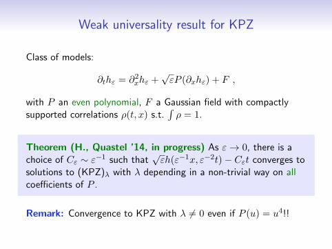
Weak universality result for KPZ
Class of models:
∂thε = ∂2xhε +√εP (∂xhε) + F ,
with P an even polynomial, F a Gaussian field with compactlysupported correlations ρ(t, x) s.t.
∫ρ = 1.
Theorem (H., Quastel ’14, in progress) As ε→ 0, there is achoice of Cε ∼ ε−1 such that
√εh(ε−1x, ε−2t)− Cεt converges to
solutions to (KPZ)λ with λ depending in a non-trivial way on allcoefficients of P .
Remark: Convergence to KPZ with λ 6= 0 even if P (u) = u4!!
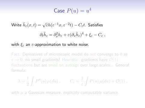
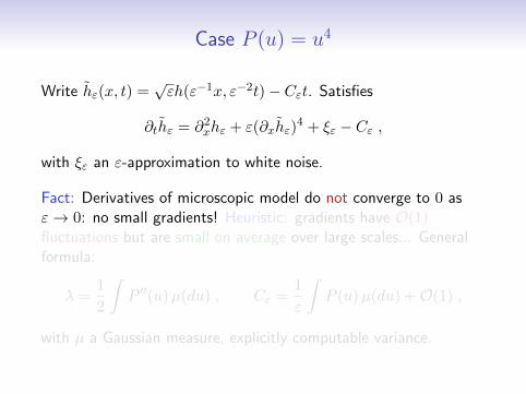
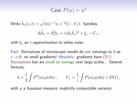
Case P (u) = u4
Write hε(x, t) =√εh(ε−1x, ε−2t)− Cεt. Satisfies
∂thε = ∂2xhε + ε(∂xhε)4 + ξε − Cε ,
with ξε an ε-approximation to white noise.
Fact: Derivatives of microscopic model do not converge to 0 asε→ 0: no small gradients! Heuristic: gradients have O(1)fluctuations but are small on average over large scales... Generalformula:
λ =1
2
∫P ′′(u)µ(du) , Cε =
1
ε
∫P (u)µ(du) +O(1) ,
with µ a Gaussian measure, explicitly computable variance.
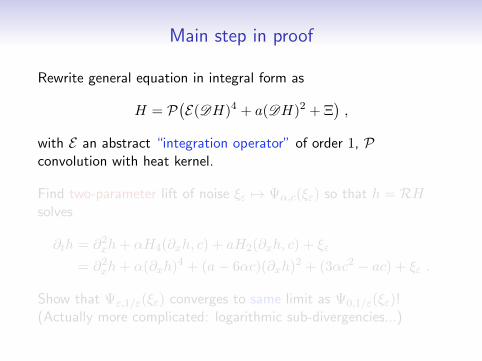
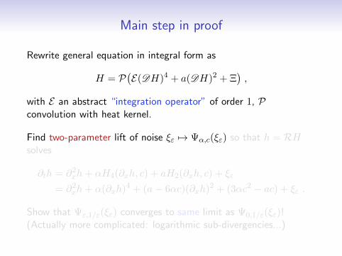
Main step in proof
Rewrite general equation in integral form as
H = P(E(DH)4 + a(DH)2 + Ξ
),
with E an abstract “integration operator” of order 1, Pconvolution with heat kernel.
Find two-parameter lift of noise ξε 7→ Ψα,c(ξε) so that h = RHsolves
∂th = ∂2xh+ αH4(∂xh, c) + aH2(∂xh, c) + ξε
= ∂2xh+ α(∂xh)4 + (a− 6αc)(∂xh)2 + (3αc2 − ac) + ξε .
Show that Ψε,1/ε(ξε) converges to same limit as Ψ0,1/ε(ξε)!(Actually more complicated: logarithmic sub-divergencies...)
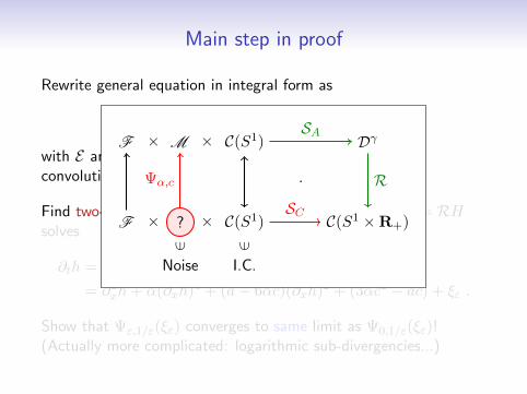
F M ×× C(S1) Dγ
·
F × ?
Noise
∈
× C(S1)
I.C.
∈C(S1 ×R+)
RΨα,c
SA
SC
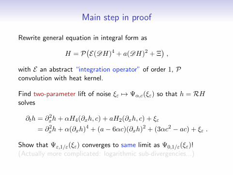
Main step in proof
Rewrite general equation in integral form as
H = P(E(DH)4 + a(DH)2 + Ξ
),
with E an abstract “integration operator” of order 1, Pconvolution with heat kernel.
Find two-parameter lift of noise ξε 7→ Ψα,c(ξε) so that h = RHsolves
∂th = ∂2xh+ αH4(∂xh, c) + aH2(∂xh, c) + ξε
= ∂2xh+ α(∂xh)4 + (a− 6αc)(∂xh)2 + (3αc2 − ac) + ξε .
Show that Ψε,1/ε(ξε) converges to same limit as Ψ0,1/ε(ξε)!(Actually more complicated: logarithmic sub-divergencies...)
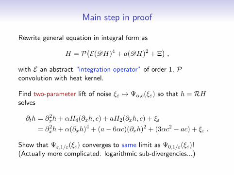
Outlook
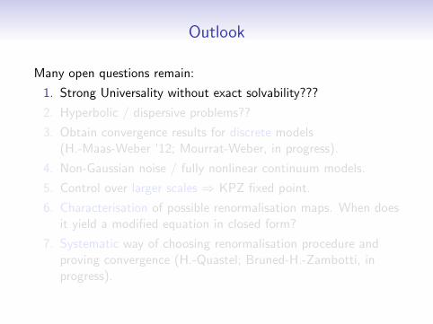
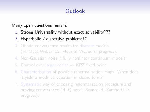
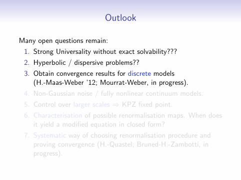
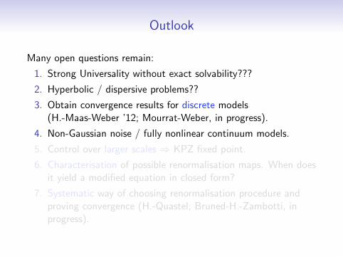
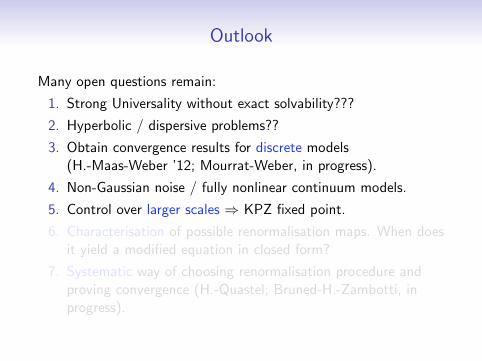
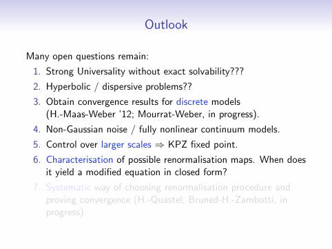
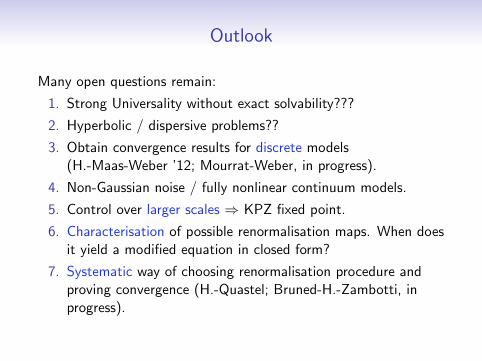
Many open questions remain:
1. Strong Universality without exact solvability???
2. Hyperbolic / dispersive problems??
3. Obtain convergence results for discrete models(H.-Maas-Weber ’12; Mourrat-Weber, in progress).
4. Non-Gaussian noise / fully nonlinear continuum models.
5. Control over larger scales ⇒ KPZ fixed point.
6. Characterisation of possible renormalisation maps. When doesit yield a modified equation in closed form?
7. Systematic way of choosing renormalisation procedure andproving convergence (H.-Quastel; Bruned-H.-Zambotti, inprogress).
Outlook
Many open questions remain:
1. Strong Universality without exact solvability???
2. Hyperbolic / dispersive problems??
3. Obtain convergence results for discrete models(H.-Maas-Weber ’12; Mourrat-Weber, in progress).
4. Non-Gaussian noise / fully nonlinear continuum models.
5. Control over larger scales ⇒ KPZ fixed point.
6. Characterisation of possible renormalisation maps. When doesit yield a modified equation in closed form?
7. Systematic way of choosing renormalisation procedure andproving convergence (H.-Quastel; Bruned-H.-Zambotti, inprogress).


![A GENERAL REGULARITY THEORY FOR WEAK MEAN … · arXiv:1111.0824v2 [math.AP] 22 Apr 2012 A GENERAL REGULARITY THEORY FOR WEAK MEAN CURVATURE FLOW KOTA KASAI AND YOSHIHIRO TONEGAWA](https://static.fdocument.org/doc/165x107/60b0c7499eaaa10450125d80/a-general-regularity-theory-for-weak-mean-arxiv11110824v2-mathap-22-apr-2012.jpg)