ByThorstenRheinlanderandMartinSchweizer¨ Technische ...
22
The Annals of Probability 1997, Vol. 25, No. 4, 1810–1831 ON L 2 -PROJECTIONS ON A SPACE OF STOCHASTIC INTEGRALS By Thorsten Rheinl ¨ ander and Martin Schweizer Technische Universit¨ at Berlin Let X be an R d -valued continuous semimartingale, T a fixed time hori- zon and the space of all R d -valued predictable X-integrable processes such that the stochastic integral Gϑ= ϑ dX is a square-integrable semimartingale. A recent paper gives necessary and sufficient conditions on X for G T to be closed in L 2 P. In this paper, we describe the structure of the L 2 -projection mapping an T -measurable random vari- able H ∈ L 2 P on G T and provide the resulting integrand ϑ H ∈ in feedback form. This is related to variance-optimal hedging strategies in financial mathematics and generalizes previous results imposing very restrictive assumptions on X. Our proofs use the variance-optimal martin- gale measure P for X and weighted norm inequalities relating P to the original measure P. 0. Introduction. Let X be an R d -valued semimartingale and the space of all R d -valued predictable X-integrable processes such that the stochastic integral Gϑ= ϑ dX is a square-integrable semimartingale. For a fixed time horizon T, G T is then a linear subspace of L 2 P, and so one can ask if there is an L 2 -projection on G T , that is, if G T is closed in L 2 P. If X is a local martingale, the answer is of course positive since the stochastic integral is then an isometry. For a continuous semimartingale X, necessary and sufficient conditions for the closedness of G T in L 2 P have recently been established by Delbaen, Monat, Schachermayer, Schweizer and Stricker (1996), subsequently abbreviated as DMSSS; see also Grandits and Krawczyk (1996) for a generalization to the case of L p P with p> 1. In this paper, we describe the structure of the L 2 -projection mapping an T - measurable random variable H ∈ L 2 P on G T and show how to obtain the integrand ϑ H ∈ appearing in this projection. If X is a local martingale, this is a classical question whose answer is given by the well-known Galtchouk– Kunita–Watanabe projection theorem. The more general semimartingale case comes up naturally in hedging problems from financial mathematics, and some partial results have been obtained by Duffie and Richardson (1991), Hipp (1993, 1996), Schweizer (1994), Wiese (1995) and Pham, Rheinl¨ ander and Schweizer (1996), among others. But all these papers imposed unnatural and very restrictive conditions on X which do not hold in typical financial models; this is discussed in more detail in Pham, Rheinl¨ ander and Schweizer (1996). Moreover, no paper so far gives a solution for H ∈ L 2 P; at least Received September 1996; revised January 1997. AMS 1991 subject classifications. 60G48, 60H05, 90A09. Key words and phrases. Semimartingales, stochastic integrals, L 2 -projection, variance-optimal martingale measure, weighted norm inequalities, Kunita–Watanabe decomposition. 1810
Transcript of ByThorstenRheinlanderandMartinSchweizer¨ Technische ...
The Annals of Probability1997, Vol. 25, No. 4, 1810–1831
ON L2-PROJECTIONS ON A SPACEOF STOCHASTIC INTEGRALS
By Thorsten Rheinlander and Martin Schweizer
Technische Universitat Berlin
LetX be an Rd-valued continuous semimartingale,T a fixed time hori-
zon and � the space of all Rd-valued predictable X-integrable processes
such that the stochastic integral G�ϑ� = ∫ϑdX is a square-integrable
semimartingale. A recent paper gives necessary and sufficient conditionson X for GT��� to be closed in L2�P�. In this paper, we describe thestructure of the L2-projection mapping an �T-measurable random vari-able H ∈ L2�P� on GT��� and provide the resulting integrand ϑH ∈ �in feedback form. This is related to variance-optimal hedging strategiesin financial mathematics and generalizes previous results imposing veryrestrictive assumptions on X. Our proofs use the variance-optimal martin-gale measure P for X and weighted norm inequalities relating P to theoriginal measure P.
0. Introduction. LetX be an Rd-valued semimartingale and � the space
of all Rd-valued predictable X-integrable processes such that the stochastic
integral G�ϑ� = ∫ϑdX is a square-integrable semimartingale. For a fixed
time horizon T, GT��� is then a linear subspace of L2�P�, and so one can askif there is an L2-projection on GT���, that is, if GT��� is closed in L2�P�. IfX is a local martingale, the answer is of course positive since the stochasticintegral is then an isometry. For a continuous semimartingale X, necessaryand sufficient conditions for the closedness of GT��� in L2�P� have recentlybeen established by Delbaen, Monat, Schachermayer, Schweizer and Stricker(1996), subsequently abbreviated as DMSSS; see also Grandits and Krawczyk(1996) for a generalization to the case of Lp�P� with p > 1.
In this paper, we describe the structure of the L2-projection mapping an �T-measurable random variableH ∈ L2�P� onGT��� and show how to obtain theintegrand ϑH ∈ � appearing in this projection. If X is a local martingale, thisis a classical question whose answer is given by the well-known Galtchouk–Kunita–Watanabe projection theorem. The more general semimartingale casecomes up naturally in hedging problems from financial mathematics, andsome partial results have been obtained by Duffie and Richardson (1991),Hipp (1993, 1996), Schweizer (1994), Wiese (1995) and Pham, Rheinlanderand Schweizer (1996), among others. But all these papers imposed unnaturaland very restrictive conditions on X which do not hold in typical financialmodels; this is discussed in more detail in Pham, Rheinlander and Schweizer(1996). Moreover, no paper so far gives a solution for H ∈ L2�P�; at least
Received September 1996; revised January 1997.AMS 1991 subject classifications. 60G48, 60H05, 90A09.Key words and phrases. Semimartingales, stochastic integrals, L2-projection, variance-optimal
martingale measure, weighted norm inequalities, Kunita–Watanabe decomposition.
1810
L2-PROJECTIONS ON STOCHASTIC INTEGRALS 1811
H ∈ L2+ε�P� is always assumed. The present paper gives the solution in thegeneral continuous L2-case.
What do we mean by “general continuous L2-case”? First of all, we assumethat X is a continuous semimartingale; any extensions to a discontinuousprocess are for the moment postponed to future research. Moreover, we onlysuppose thatH ∈ L2�P�. The basic idea for attacking the problem is to connectthe semimartingale to the martingale case in some way, and this is achieved byassuming that there exists an equivalent local martingale measure (ELMM,for short) forX, that is, a probability measureQ equivalent toP such thatX isa localQ-martingale. This is a well-known condition in financial mathematics,which states that X should not allow arbitrage opportunities. By Girsanov’stheorem, the existence of an ELMM implies that the canonical decompositionof X must have the form
X =X0 +M+∫d�M�λ
for some predictable process λ. Again by Girsanov’s theorem, a natural candi-date for an ELMM is then given by the so-called minimal martingale measureP with density
dP
dP= �
(−∫λdM
)T
�
The main results in the existing literature show that the integrand ϑH of Xin the projection of H on GT��� can be written in feedback form as
�0�1� ϑH = ξ H − ζ
Z
(VH
− −∫ϑH dX
)�
where VH is the P-martingale
�0�2� VHt = EH�t�� 0 ≤ t ≤ T
and ξ H is the integrand of X in the Galtchouk–Kunita–Watanabe decompo-sition of H under P. The crucial assumption for this to be true is that thedensity of P can be written as a constant plus a stochastic integral of X,
�0�3� dP
dP= E
[dP
dP
]+
∫ T0ζs dXs
for some ζ ∈ �, and the process Z in (0.1) is then
�0�4� Zt = E
[dP
dP
∣∣∣∣�t]= E
[dP
dP
]+
∫ t0ζs dXs� 0 ≤ t ≤ T�
In addition, one has to impose moment conditions on H and dP/dP since(0.1) is proved by switching from P to P and back, and one needs squareintegrability under P for this method to work.
1812 T. RHEINLANDER AND M. SCHWEIZER
As pointed out in Pham, Rheinlander and Schweizer (1996), the minimalmartingale measure P will typically not satisfy (0.3) so that the precedingresult has a very limited scope. But there is another ELMM whose densityalmost by definition does satisfy the requirement (0.3). This is the variance-optimal martingale measure P defined by the property that its density withrespect toP has minimalL2�P�-norm among all ELMMs forX. Due to a resultof Delbaen and Schachermayer (1996), P always exists if X is continuous andif there is at least one ELMM for X with density in L2�P�. In this paper,we show that these two conditions plus closedness of GT��� in L2�P� arealready sufficient to obtain ϑH in feedback form. More precisely, we show thatunder these assumptions, (0.1)–(0.4) always hold if we replace the minimalmartingale measure throughout by the variance-optimal martingale measureand every hat by a tilde ˜. Moreover, no assumption on H is needed except,of course, H ∈ L2�P�.
The main tools to obtain these results are weighted norm inequalities whichallow us to obtain estimates in L2�P� for processes which are local martin-gales under P. This is possible thanks to the main result of DMSSS, whichcharacterizes the closedness of GT��� by the validity of such inequalities. Sec-tion 1 contains a precise formulation of the basic problem and a brief surveyof those results of DMSSS that we use in this paper. In Section 2, we studythe properties of the Galtchouk–Kunita–Watanabe decomposition of H underan ELMM Q, and we show that the terms in this decomposition have goodproperties in L2�P� if one has weighted norm inequalities linking P and Q.Any such Q then leads to a decomposition of H into a constant, an integral inGT��� and a certain orthogonal term, and it remains to project constants andthose orthogonal terms on GT���. By the definition of P, the density dP/dPis a multiple of the projection of the constant 1 on the orthogonal complementof GT��� in L2�P�, and this suggests working with Q = P to effect the decom-position of H. In Section 3, we show that this does indeed give the solutionand leads to the representation of ϑH as in (0.1). An alternative approach todetermine the integrand ϑH has recently been proposed by Gourieroux, Lau-rent and Pham (1996). We briefly discuss their main result in Section 4, and,because this is not clear from their formulation, we prove that they do indeedsolve the same problem as in our paper.
1. Preliminaries. Let ���� �F�P� be a filtered probability space with afiltration F = ��t�0≤t≤T satisfying the usual conditions, where T ∈ �0�∞� is afixed time horizon. For simplicity, we assume that �0 is trivial and � = �T. Allstochastic processes will be indexed by t ∈ 0�T�. Let X be a continuous R
d-valued semimartingale with canonical decompositionX =X0+M+A. For anyRd-valued predictable X-integrable process ϑ, we denote by G�ϑ� the (real-
valued) stochastic integral process G�ϑ� �= ∫ϑdX. Unexplained terminology
and notation from martingale theory can be found in Dellacherie and Meyer(1982). Throughout the paper, C denotes a generic constant in �0�∞� whichmay vary from line to line.
L2-PROJECTIONS ON STOCHASTIC INTEGRALS 1813
Definition. For any RCLL process Y, we denote by Y∗t �= sup0≤s≤t Ys
the supremum process of Y. The space �2�P� consists of all adapted RCLLprocesses Y such that
�Y��2�P� �= �Y∗T�L2�P� <∞�
Definition. Let L2�M� be the space of all Rd-valued predictable processes
ϑ such that
�ϑ�2L2�M� �= E
[∫ T0ϑtrt d�M�t ϑt
]<∞�
Let L2�A� be the space of all Rd-valued predictable processes ϑ such that
�ϑ�2L2�A� �= E
[(∫ T0
∣∣ϑtrt dAt
∣∣)2]<∞�
Finally, we set � �= L2�M� ∩L2�A�.
If ϑ is in �, the continuous semimartingale G�ϑ� is in �2�P� so that inparticular its terminal value GT�ϑ� is in L2�P�. For any given H ∈ L2�P�, wemay thus consider the optimization problem
�1�1� Minimize �H−GT�ϑ��L2�P� over all ϑ ∈ ��To ensure that (1.1) has a solution for everyH ∈ L2�P�, we impose throughoutthis paper the standing assumption
�1�2� GT��� is closed in L2�P��Necessary and sufficient conditions on X to guarantee (1.2) were establishedin DMSSS, and we briefly summarize here those results we shall use in thepresent paper.
Definition. Let Z be a uniformly integrable martingale with Z0 = 1 andZT > 0. We say that Z satisfies the reverse Holder inequality with exponentp ∈ �1�∞� under P, denoted by Rp�P�, if there is a constant C such that forevery stopping time S ≤ T, we have
E
[(ZT
ZS
)p∣∣∣∣�S]≤ C�
Definition. Let Z be an adapted RCLL process. We say that Z satisfiescondition �J� if there is a constant C such that
1CZ− ≤ Z ≤ CZ−�
Definition. If Q is a probability measure equivalent to P, we denote byZQ an RCLL version of the strictly positive P-martingale
ZQt �= EP
[dQ
dP
∣∣∣∣�t]� 0 ≤ t ≤ T�
1814 T. RHEINLANDER AND M. SCHWEIZER
With these definitions in place, we can now recall two fundamental weightednorm inequalities. The first one is a consequence of Propositions 4 and 5 andthe Corollary on page 318 of Doleans-Dade and Meyer (1979); the second onefollows by a localization argument from Theorem 2 of Bonami and Lepingle(1979), combined with Proposition 5 of Doleans-Dade and Meyer (1979).
Proposition 1. LetQ be a probability measure equivalent toP and assumethat ZQ satisfies R2�P� and �J�. Then we have the following.
(i) There exists a constant C such that
E[�N∗
S�2] ≤ CE[N2S
]for all uniformly integrable Q-martingales N and all stopping times S ≤ T.
(ii) There exist two constants c and C in �0�∞� such that
cE[�N∗
S�2] ≤ EN�S� ≤ CE[�N∗
S�2]for all local Q-martingales N and all stopping times S ≤ T.
Note that (i) and (ii) are generalizations of the Doob and Burkholder–Davis–Gundy inequalities, respectively, since we have estimates in the L2-norm un-der P for processes which are local martingales under Q.
To relate Proposition 1 to the closedness of GT��� in L2�P�, we recall theconcept of the variance-optimal martingale measure which was studied inDelbaen and Schachermayer (1996) and Schweizer (1996). Let � denote thelinear subspace of L∞���� �P� spanned by the simple stochastic integralsof the form Y = htr�XT2
− XT1�, where T1 ≤ T2 ≤ T are stopping times
such that the stopped process XT2 is bounded and h is a bounded Rd-valued
�T1-measurable random variable.
Definition. Let � s�P� be the space of all signed measures Q � P withQ�� = 1 and
E
[dQ
dPY
]= 0 for all Y ∈ � �
Let � e�P� denote the subset of all probability measures Q ∈ � s�P� such thatQ is equivalent to P. Finally, we define two sets of densities by
�x �={dQ
dP
∣∣∣∣Q ∈ � x�P�}
for x ∈ �e� s��
It is clear that X is a local Q-martingale for any Q ∈ � e�P� and that � s ∩L2�P� is a closed convex set.
Definition. The variance-optimal martingale measure P is the uniqueelement of � s�P� such that D = dP/dP is in L2�P� and minimizes �D�L2�P�over all D ∈ � s ∩L2�P�.
L2-PROJECTIONS ON STOCHASTIC INTEGRALS 1815
Note that P exists if and only if � s ∩L2�P� is nonempty. In that case, wedefine Z and Z as RCLL versions of
Zt �= E
[dP
dP
∣∣∣∣�t]= ZP
t � 0 ≤ t ≤ T
and
Zt �= E
[dP
dP
∣∣∣∣�t]� 0 ≤ t ≤ T�
where E denotes expectation with respect to P. Since X is continuous, The-orem 1.3 of Delbaen and Schachermayer (1996) implies that P is actually in� e�P� as soon as it exists. In particular, � e ∩L2�P� is nonempty as soon as� s ∩ L2�P� is. The following result is then a partial statement of Theorem4.1 of DMSSS, combined with their Lemma 2.17, Theorem 3.7, Lemma 3.2,Theorem 2.22 and Theorem 1.3 of Delbaen and Schachermayer (1996); L∞
+ �P�denotes the space of all nonnegative bounded random variables.
Theorem 2. For a continuous semimartingale X, the following conditionsare equivalent.
(i) GT��� is closed in L2�P�, and GT��� ∩L∞+ �P� = �0�.
(ii) GT��� is closed in L2�P�, and � s ∩L2�P� �= �.
(iii) The variance–optimal martingale measure P exists and is in � e�P�,and Z = ZP satisfies the reverse Holder inequality R2�P�.Moreover, each of these conditions implies that Z satisfies condition �J� andthat � = L2�M�.
We conclude this section with a simple observation from DMSSS, whichturns out to be extremely useful in the sequel. If P exists, the Bayes ruleyields
Zt = E[ZT
∣∣�t] = 1Zt
E[Z2T
∣∣�t] = 1Zt
E[Z2T
∣∣�t]�If Z satisfies R2�P�, we have from Jensen’s inequality
1 ≤ 1
Z2t
E[Z2T
∣∣�t] ≤ C�and therefore
�1�3� Zt ≤ Zt ≤ CZt�
The importance of this comparison lies in the fact that it will allow us toswitch freely between Z and Z for the purposes of estimation.
1816 T. RHEINLANDER AND M. SCHWEIZER
2. Kunita–Watanabe decompositions under a change of measure.Let Q be an equivalent local martingale measure for X, that is, a probabil-ity measure equivalent to P such that X is a local Q-martingale. Since X iscontinuous, every local Q-martingale admits a Galtchouk–Kunita–Watanabedecomposition with respect to X under Q into a stochastic integral of X and alocal Q-martingale strongly Q-orthogonal to X; see Ansel and Stricker (1993).Our main result in this section shows that a control on the density process ZQ
allows us to obtain good integrability properties under the original measureP for this decomposition.
Theorem 3. Assume (1.2) as well as � s ∩ L2�P� �= �. Let dQ/dP ∈ � e ∩L2�P� be such that the associated density process ZQ satisfies R2�P� and �J�.For any H ∈ L2�P�, define the Q-martingale VH�Q as an RCLL-version of
VH�Qt �= EQH�t�. Then there exist a process ξH�Q ∈ � and a Q-martingale
LH�Q null at 0 with LH�Q ∈ �2�P� and
�2�1� [LH�Q�Xi
] = 0 for i = 1� � � � � d
such that VH�Q can be uniquely written as
VH�Qt = EQH� +
∫ t0ξH�Qs dXs +LH�Qt � 0 ≤ t ≤ T�
Proof. Since X is a continuous local Q-martingale, we know from Anseland Stricker (1993) that VH�Q has a unique Galtchouk–Kunita–Watanabedecomposition with respect to X under Q. More precisely, there exist an R
d-valued predictable X-integrable process ξH�Q and a local Q-martingale LH�Q
null at 0 with
VH�Q = EQH� +∫ξH�Q dX+LH�Q
and such that LH�Q�Xi� is a local Q-martingale for i = 1� � � � � d. Since X iscontinuous, we have[
LH�Q�Xi] = ⟨
LH�Q�Xi⟩ = 0 for i = 1� � � � � d
and therefore (2.1). By definition, VH�Q is a uniformly integrable Q-mar-tingale. Because ZQ satisfies R2�P� and �J�, Proposition 1 implies that
E[[VH�Q
]T
] ≤ CE[sup
0≤t≤T
∣∣VH�Qt
∣∣2] ≤ CE[(VH�QT
)2] = CEH2� <∞�
By (2.1) and the continuity of X,[VH�Q
] = ∫ (ξH�Q
)trd�M� ξH�Q + [
LH�Q]�
and so we conclude that ξH�Q is in L2�M�, hence in � by Theorem 2. Moreover,LH�Q is a local Q-martingale with LH�Q�T ≤ VH�Q�T ∈ L1�P�, and so LH�Q
is in �2�P� by part (ii) of Proposition 1. Since dQ/dP is in L2�P�, this finallyimplies that the local Q-martingale LH�Q is in fact a true Q-martingale. ✷
L2-PROJECTIONS ON STOCHASTIC INTEGRALS 1817
Remark. If the minimal martingale measure P happens to satisfy the as-sumptions of Theorem 3, the above decomposition for Q = P will coincidewith the Follmer–Schweizer decomposition of H; see Schweizer (1995a). ForQ �= P, we obtain in general a different decomposition. Moreover, it mayhappen that GT��� is closed and that the variance-optimal martingale mea-sure P satisfies R2�P�, while P fails to satisfy R2�P�; see Example 3.12 ofDMSSS. Together with the development in the next section, this shows thatthe Follmer–Schweizer decomposition is in general not the appropriate tool tosolve the optimization problem (1.1).
3. The integrand in the L2-projection on GT���. Consider now a fixedrandom variable H ∈ L2�P�. Thanks to the standing assumption (1.2), we canproject H in L2�P� on GT��� so that (1.1) has a solution which we denote byϑH ∈ �. Although the random variable GT�ϑH� is uniquely determined, ϑH
itself need not be unique, but it will be as soon as the mapping ϑ �→ GT�ϑ� isinjective. According to Lemma 3.5 of DMSSS, this is the case if � e ∩L2�P� isnonempty, and so we shall adopt this assumption in addition to (1.2).
In order to determine ϑH, we can use Theorem 3 to decompose H into threeterms and to project these on GT��� separately. The middle term is already inGT��� for any suitable choice of Q in Theorem 3. The first term is a constant,and so its projection will be directly related to the density of the variance-optimal martingale measure P. This suggests working withQ = P in Theorem3, an intuition supported by the results obtained in Pham, Rheinlander andSchweizer (1996), and we shall see that Q = P is indeed the right choice.
According to the projection theorem, a process ϑH ∈ � solves (1.1) if andonly if
�3�1� E[(H−GT�ϑH�
)GT�ϑ�
] = 0 for all ϑ ∈ ��
By Theorem 2, the density process Z = ZP of P satisfies R2�P� and condition�J�, and so Theorem 3 allows us to write H as
�3�2� H = EH� +∫ T
0ξHs dXs + LHT
for a process ξH ∈ � and a P-martingale LH null at 0 with LH ∈ �2�P� and
�3�3� [LH�Xi
] = 0 for i = 1� � � � � d�
By Lemma 1 of Schweizer (1996), the density of P with respect to P can bewritten as
dP
dP= E
[dP
dP
]+
∫ T0ζs dXs for some ζ ∈ ��
1818 T. RHEINLANDER AND M. SCHWEIZER
and so we have
�3�4� Zt = E
[dP
dP
∣∣∣∣�t]= EZT� +
∫ t0ζs dXs� 0 ≤ t ≤ T�
This shows in particular that the P-martingale Z is continuous and stronglyP-orthogonal to a local P-martingale L if and only if L is strongly P-orthogonal to X.
Lemma 4. Assume (1.2) as well as � s ∩ L2�P� �= �. Then we have thefollowing.
(i) For H ≡ 1, the solution ϑH of (1.1) is given by
ϑH = −Z−10 ζ�
(ii) For H = ∫ T0 ξ
Hs dXs with ξH ∈ �, the solution ϑH of (1.1) is given by
ϑH = ξH�
Proof. Since (ii) is obvious, we only have to prove (i). Property (3.4) of thevariance-optimal martingale measure implies that
H = 1 = Z−10 ZT −
∫ T0Z−1
0 ζs dXs�
and by the definition of P, ZT is in the orthogonal complement of GT��� inL2�P�. Since Z−1
0 ζ is in �, the assertion follows from (3.1). ✷
In view of the preceding discussion, it now remains to consider the casewhere H = LHT . This is actually the hardest case, and the next theorem canin a sense be viewed as the main result of this paper.
Theorem 5. Assume (1.2) and � s ∩ L2�P� �= �. Let H ∈ L2�P� be such
that the P-martingale L defined by Lt �= EH�t� is null at 0 and satisfies
L�Xi� = 0 for i = 1� � � � � d. Then the solution ϑH of (1.1) is given by
ϑHt = −ζt∫ t−
0Z−1s dLs�
Proof. Since L�Xi� = 0 for i = 1� � � � � d, (3.4) implies that L� Z� = 0. Ifwe define the R
d-valued predictable X-integrable process ϑ by
ϑt �= −ζt∫ t−
0Z−1s dLs�
the product rule and (3.4) therefore imply that
�3�5�∫ϑ dX = L− Z
∫Z−1 dL�
L2-PROJECTIONS ON STOCHASTIC INTEGRALS 1819
The subsequent Lemma 7 will show that
�3�6� Z∫Z−1 dL ∈ �2�P��
By Theorem 3, L ∈ �2�P�, and so (3.5) and (3.6) show that the local P-martingale
∫ϑ dX is also in �2�P�. Proposition 1 and the continuity of X
thus imply that
∫ T0ϑtrt d�M�t ϑt =
∫ T0ϑtrt dX�t ϑt =
[∫ϑ dX
]T
∈ L1�P��
and so ϑ is in L2�M� = � by Theorem 2. To complete the proof, it thusremains to show that ϑ satisfies (3.1). Now the product rule and L�Xi� = 0for i = 1� � � � � d imply that for ϑ ∈ �, the process G�ϑ� ∫ Z−1 dL is a local P-martingale, and so ZG�ϑ� ∫ Z−1 dL is a local P-martingale. We now use (1.3)to replace Z by Z, then (3.6), the fact that G�ϑ� ∈ �2�P� and the Cauchy–Schwarz inequality to finally obtain
sup0≤t≤T
∣∣∣∣ZtGt�ϑ�∫ t
0Z−1s dLs
∣∣∣∣ ∈ L1�P��
and so ZG�ϑ� ∫ Z−1 dL is even a true P-martingale for every ϑ ∈ �. SinceZT = ZT, (3.5) and LT =H imply that
E[�H−GT�ϑ��GT�ϑ�
] = E
[ZTGT�ϑ�
∫ T0Z−1s dLs
]= 0 for all ϑ ∈ ��
which proves that ϑ solves the optimization problem (1.1). ✷
Now define the process VH by setting
�3�7� VHt �= EH� +
∫ t0ξHs dXs + LHt = EH�t�� 0 ≤ t ≤ T�
Putting everything together, we then obtain the following result.
Theorem 6. Assume (1.2) and � s ∩ L2�P� �= �. For any H ∈ L2�P�, thesolution of (1.1) takes the form�3�8�
ϑHt = ξHt − ζt(EH�Z−1
0 +∫ t−
0Z−1s dLHs
)= ξHt − ζt
Zt
(VHt− −
∫ t0ϑHs dXs
)�
Proof. Due to the linearity of H �→ ϑH, the first equality is immediatefrom Lemma 4 and Theorem 5. Since LH� Z� = 0 by (3.4) and (3.3), we can
1820 T. RHEINLANDER AND M. SCHWEIZER
use the product rule, (3.4) and the first equality in (3.8) to obtain
Z
(EH�Z−1
0 +∫Z−1 dLH
)= EH� +
∫EH�Z−1
0 ζ dX
+∫ (∫
Z−1 dLH)−ζ dX+ LH
= EH� + LH +∫ (ξH −ϑH)dX
= VH −∫ϑH dX�
and this yields the second equality in (3.8). ✷
Remark. The second expression for ϑH in (3.8) gives us the optimal inte-grand in feedback form, with a correction term which is proportional to theamount by which the cumulative gains from trade
∫ϑH dX deviate from the
current intrinsic P-value VH of H in (3.7). This generalizes results of variousauthors where this representation was only obtained under very restrictive ad-ditional conditions. Duffie and Richardson (1991) and Schweizer (1994) workedwith a “deterministic mean-variance tradeoff,” while Hipp (1993, 1996), Wiese(1995) and Pham, Rheinlander and Schweizer (1996) assumed somewhat moregenerally that the minimal martingale measure P coincides with the variance-optimal martingale measure P. But all these assumptions are quite unnaturaland will fail in most typical situations; see Pham, Rheinlander and Schweizer(1996) for an amplification of this point.
It now remains to prove the crucial estimate (3.6), and this is indeed wherethe main work has to be done. The key observation in the following proof isthat the stochastic integral
∫Z−1 dL can equivalently be written as a back-
ward integral, which is possible thanks to the orthogonality of L and X andthe property (3.4) of the variance-optimal martingale measure. This alterna-tive representation allows us in turn to apply the reverse Holder inequalityR2�P� backward in time to obtain the desired estimate by an approximationprocedure. The original motivation for looking at the problem in this waycomes from Schweizer (1995b) where a backward induction argument is usedto solve the optimization problem (1.1) in finite discrete time. By using a suit-able change of measure, we are able to give an alternative shorter proof inSection 4.2. On the other hand, the subsequent argument has the advantagethat all computations and estimates are made under the original measureP, and this appears more promising in view of possible generalizations to adiscontinuous process X.
Lemma 7. With the assumptions and notations of Theorem 5, we have
�3�6� sup0≤t≤T
∣∣∣∣Zt
∫ t0Z−1s dLs
∣∣∣∣ ∈ L2�P��
L2-PROJECTIONS ON STOCHASTIC INTEGRALS 1821
Proof. For brevity, let us write N �= Z∫Z−1dL. By (3.5), N is a local
P-martingale so that we can choose an increasing sequence �Tn� of stoppingtimes such that NTn is a uniformly integrable P-martingale. From part (i) ofProposition 1, we get
E[
sup0≤t≤T
∣∣NTnt
∣∣2] ≤ CE[N2Tn
]for a constant C which does not depend on n, and so it is enough to show that
�3�9� supS
E[N2S
]<∞�
where the supremum runs over all stopping times S ≤ T. The assertion thenfollows by letting n tend to infinity and applying the monotone convergencetheorem.
To prove (3.9), we shall first show that
�3�10� E[N2S
] ≤ CEL�S�for any stopping time S ≤ T, with a constant C which does not depend on S.Theorem 2 and Proposition 1 then imply that
supS
E[N2S
] ≤ CEL�T� ≤ CE[
sup0≤t≤T
L2t
]≤ CE[
L2T
] = CEH2� <∞�
which gives (3.9).As a preparation for the proof of (3.10), we now fix a stopping time S ≤ T
and approximate the stochastic integral∫ S
0 Z−1u dLu appearing in NS. A
random partition of 0� S�� is a finite family σ of stopping times Ti suchthat 0 = T0 ≤ T1 ≤ · · · ≤ Tk = S P-a.s.; its (random) grid size isσ �= maxi=1�����k Ti − Ti−1. According to Theorems II.21 and II.23 ofProtter (1990), there exists a sequence �σm�m∈N of random partitions of0� S�� with limm→∞ σm = 0 P-a.s. such that∫ S
0Z−1u dLu = lim
m→∞∑
Ti∈σmZ−1Ti
(LTi+1
− LTi)
in probability
as well as[Z−1� L
]S= lim
m→∞∑
Ti∈σm
(Z−1Ti+1
− Z−1Ti
)(LTi+1
− LTi)
in probability.
But Z−1� L� = 0 by Ito’s formula since Z is continuous and Z� L� = 0 as inthe proof of Theorem 5. Hence we get by addition
�3�11�∫ S
0Z−1u dLu = lim
m→∞∑
Ti∈σmZ−1Ti+1
(LTi+1
− LTi)
in probability,
and this shows that the forward integral∫Z−1 dL can also be written as a
backward integral∫Z−1 d∗L.
1822 T. RHEINLANDER AND M. SCHWEIZER
According to (1.3) and the definition of N, proving (3.10) is equivalent toshowing that
�3�12� E
[ZSZS
(∫ S0Z−1u dLu
)2]≤ CEL�S��
If Ti�Ti+1�Tj�Tj+1 are stopping times with 0 ≤ Ti ≤ Ti+1 ≤ Tj ≤ Tj+1 ≤ S,we have
E
[ZSZS
�LTi+1− LTi�
ZTi+1
�LTj+1− LTj�
ZTj+1
]
= E
[�LTi+1− LTi�
ZTi+1
E
[ZSZS
�LTj+1− LTj�
ZTj+1
∣∣∣∣�Tj]]
= 0�
In fact, ZZ is a P-martingale because Z is a P-martingale; thus we obtain
E
[ZSZS
�LTj+1− LTj�
ZTj+1
∣∣∣∣�Tj]= E
[ZTj+1
(LTj+1
− LTj)∣∣�Tj] = 0
by first conditioning on �Tj+1and then using the fact that ZL is a P-
martingale because L is a P-martingale. If we approximate∫ S
0 Z−1u dLu as
in (3.11), the mixed terms appearing in the corresponding approximation of(3.12) thus have expectation 0, and so we obtain
supmE
[ZSZS
( ∑Ti∈σm�S�
Z−1Ti+1
(LTi+1
− LTi))2]
= supmE
[ ∑Ti∈σm�S�
ZSZS
Z2Ti+1
(LTi+1
− LTi)2]
≤ C supmE
[ ∑Ti∈σm�S�
Z2S
Z2Ti+1
(LTi+1
− LTi)2]
= C supmE
[ ∑Ti∈σm�S�
(LTi+1
− LTi)2E
[Z2S
Z2Ti+1
∣∣∣∣�Ti+1
]]
≤ C supmE
[ ∑Ti∈σm�S�
(LTi+1
− LTi)2]
≤ C supmE
[ ∑Ti∈σm�S�
(L�Ti+1− L�Ti
)]
≤ CEL�S��where we have used (1.3), the reverse Holder inequality R2�P� and Proposi-tion 1. In particular, the third inequality is obtained by applying part (ii) of
L2-PROJECTIONS ON STOCHASTIC INTEGRALS 1823
Proposition 1 to the finitely many P-martingales Ni �= LTi+1 − LTi . Note alsothat none of the appearing constants depends on m or on the stopping timeS. By (3.11),
limm→∞ZSZS
( ∑Ti∈σm�S�
Z−1Ti+1
(LTi+1
− LTi))2
= ZSZS
(∫ S0Z−1s dLs
)2
in probability,
and so Fatou’s lemma yields (3.12). This completes the proof. ✷
4. A second solution. A very elegant different method of attacking thebasic problem (1.1) has recently been proposed by Gourieroux, Laurent andPham (1996), subsequently abbreviated as GLP. Their idea is to combine achange of measure with a change of coordinates to transform the problem insuch a way that it can be solved directly by means of the Galtchouk–Kunita–Watanabe projection theorem. But a priori, GLP are only able to solve a weakerproblem by their approach, and one contribution of the present paper is toprove that they actually obtain the solution to the same question that weconsider here.
4.1. The alternative approach. This subsection briefly explains the resultsof GLP. Their basic model is a multidimensional diffusion model with a Brown-ian filtration. The R
d+1-valued process S is given by
dS0t
S0t
= rt dt� S00 = 1
and
dSit
Sit= µit dt+
n∑j=1
σijt dW
jt � Si0 > 0
for i = 1� � � � � d ≤ n, with predictable processes r, µ, σ satisfying appropriateintegrability conditions. The process X is then the R
d-valued process withcomponents Xi �= Si/S0 for i = 1� � � � � d. To facilitate comparisons and toavoid some technical problems, we consider in the sequel the discounted casewhere r ≡ 0 so that S0 ≡ 1. Our subsequent arguments do not need thediffusion structure, but only the continuity of X.
Denote as above by P the variance-optimal martingale measure for X sothatX is a continuous local P-martingale. GLP then consider the optimizationproblem
�4�1� Minimize �H−GT�ϑ��L2�P� over all ϑ ∈ ��
where the space � consists of all Rd-valued predictableX-integrable processes
ϑ such that the stochastic integral G�ϑ� is a P-martingale satisfying GT�ϑ� ∈
1824 T. RHEINLANDER AND M. SCHWEIZER
L2�P�. It is easy to check (and will be proved in Lemma 9) that � is thencontained in � so that (4.1) is more likely to have a solution than (1.1).
Now consider the strictly positive P-martingale Z given by (3.4) and definea new probability measure R ≈ P by setting
dR
dP�= ZT
Z0
= 1 +∫ T
0Z−1
0 ζs dXs�
Since X is a continuous local P-martingale, the Rd+1-valued process Y
with Y0 �= Z−1 and Yi �= XiZ−1 for i = 1� � � � � d is a continuous localR-martingale. Moreover,
�4�2� dR
dP= dR
dP
dP
dP= Z2
T
Z0
�
and so we obtain
�4�3� ∥∥H−GT�ϑ�∥∥L2�P� =
√Z0
∥∥∥∥ HZT
− GT�ϑ�ZT
∥∥∥∥L2�R�
�
A generalized version of the crucial result of GLP is then
Proposition 8. Assume that X is a continuous semimartingale which sat-isfies (1.2) and � s ∩L2�P� �= �. Then
�4�4� 1
ZT
GT��� ={∫ T
0ψu dYu
∣∣∣∣ψ ∈ L2�Y� R�}�
where L2�Y� R� is the space of all Rd+1-valued predictable Y-integrable pro-
cesses ψ such that∫ψdY is in the space � 2�R� of martingales. Moreover, the
relation between ϑ ∈ � and ψ ∈ L2�Y� R� is given by
�4�5�ψi �= ϑi for i = 1� � � � � d�
ψ0 �= G�ϑ� −ϑtrX
and
�4�6� ϑi �= ψi + ζi(∫
ψdY− ψtrY
)for i = 1� � � � � d�
Proof. The crucial step of the argument is to show that
�4�7�
{G�ϑ�∣∣ϑ is R
d-valued, predictable and X-integrable}
={Z
∫ψdY
∣∣∣∣ψ is Rd+1-valued, predictable and Y-integrable
}with the relation between ϑ and ψ given by (4.5) and (4.6). As a preparationfor this, note first that the product rule yields
�4�8� d(XZ−1) = Z−1 dX+XdZ−1 + d[X� Z−1]�
L2-PROJECTIONS ON STOCHASTIC INTEGRALS 1825
�4�9�d(G�ϑ�Z−1) = Z−1 dG�ϑ� +G�ϑ�dZ−1 + d[G�ϑ�� Z−1]
= Z−1ϑdX+G�ϑ�dZ−1 +ϑtr d[X� Z−1]
and
�4�10� d�ZY� = YdZ+ Z dY+ dZ�Y��Suppose first that ϑ is X-integrable and define ϑn �= ϑI�ϑ≤n�. Then (4.9),
(4.8) and the definition of Y imply that
d(G�ϑn�Z−1) = Z−1ϑn dX+G�ϑn�dZ−1 + �ϑn�trd
[X� Z−1]
= ϑn d(XZ−1)+ (
G�ϑn� − �ϑn�trX)dZ−1
= (ψ�n�)dY�
where the Y-integrable process ψ�n� is given by
�ψ�n��0 �= G�ϑn� − �ϑn�trX�
�ψ�n��i �= �ϑn�i for i = 1� � � � � d�
As n tends to infinity, G�ϑn� converges to G�ϑ� in the semimartingale topol-ogy because ϑ is X-integrable. This implies that
∫ψ�n� dY = Z−1G�ϑn� also
converges in the semimartingale topology since multiplication with a fixedsemimartingale is a continuous operation; see Proposition 4 of Emery (1979).By Theorem V.4 of Memin (1980), the subspace �∫ ψdYψ is Y-integrable� isclosed in the semimartingale topology, and so we conclude that
Z−1G�ϑ� =∫ψ dY for some Y-integrable process ψ.
But since ψ�n� converges for n → ∞ (P-a.s. uniformly in t, at least along asubsequence) to ψ given by (4.5), we deduce from Theorem V.4 of Memin (1980)that ψ = ψ, and this establishes the inclusion “⊆” in (4.7).
The proof of the converse is very similar. If ψ is Y-integrable, we defineψn �= ψI�ψ≤n� and use the product rule, (3.4), (4.10) and the definition of Yto obtain
d
(Z
∫ψn dY
)=
(∫ψn dY
)dZ+ Zψn dY+ �ψn�tr dZ�Y�
=(∫
ψn dY
)ζ dX+ ψn d�ZY� − (�ψn�trY
)dZ
= ϑ�n� dX
with the X-integrable process
�ϑ�n��i �= �ψn�i + ζi(∫
ψn dY− �ψn�trY
)for i = 1� � � � � d�
1826 T. RHEINLANDER AND M. SCHWEIZER
An analogous argument as above then yields for n→ ∞ that
Z∫ψdY = G�ϑ�
with ϑ given by (4.6), and this establishes the inclusion “⊇” in (4.7).The proof of (4.4) is now easy. For ψ ∈ L2�Y� R�, the stochastic integral∫ψdY is an R-martingale so that the product Z
∫ψdY = G�ϑ� is a P-
martingale. Moreover, (4.2) and (4.7) yield
E�GT�ϑ��2� = Z0ER
[(∫ T0ψu dYu
)2]<∞
since∫ψdY ∈ � 2�R�, and so GT�ϑ� is in L2�P�. Conversely, let G�ϑ� be
a P-martingale with terminal value GT�ϑ� ∈ L2�P�. Then (4.7) shows that∫ψdY is an R-martingale whose terminal value GT�ϑ�/ZT is in L2�R� due
to (4.2). Hence ψ must be in L2�Y� R�, and this completes the proof. ✷
In view of Proposition 8 and (4.3), (4.1) is equivalent to the optimizationproblem
�4�11� Minimize∥∥∥∥ HZT
−∫ T
0ψu dYu
∥∥∥∥L2�R�
over all ψ ∈ L2�Y� R��
But this is a much easier problem. In fact, since Y is an R-martingale, thesolution ψ∗ of (4.11) is simply given by the integrand of Y in the Galtchouk–Kunita–Watanabe decomposition under R of the random variable H/ZT ∈L2�R�. The solution ϑ∗ of (4.1) is then obtained via (4.6). The transformationfrom X to Y and back is the change of coordinates alluded to above.
Remarks. (i) A result similar to Proposition 8 is given in GLP for themultidimensional diffusion case under the assumptions that σσ tr is invertibleand that σ tr�σσ tr�−1�µ−r1� is bounded. This amounts to saying that X has abounded mean-variance tradeoff which is a well-known convenient condition.It is sufficient (but not necessary) to ensure that GT��� is closed in L2�P� andthat � s ∩ L2�P� contains the density of the minimal martingale measure Pand is therefore nonempty; see DMSSS for more details.
(ii) A closer look at the proof of Proposition 8 shows that we do not reallyneed the assumption (1.2) that GT��� is closed in L2�P�. All we require is theexistence of the variance-optimal martingale measure P and the representa-tion
Zt = EZT� +∫ t
0ζs dXs� 0 ≤ t ≤ T
for some X-integrable process ζ (which need not even be in �). By Lemma 2.2of Delbaen and Schachermayer (1996), this is satisfied as soon as � e ∩L2�P�is nonempty. In particular, Proposition 8 then implies that GT��� is closed in
L2-PROJECTIONS ON STOCHASTIC INTEGRALS 1827
L2�P� so that (4.1) is indeed easier to solve than (1.1). (We are grateful toL. Krawczyk for this remark.)
4.2. The relation to our results. Let us now compare our results to thoseof GLP. As pointed out in GLP, the solution ϑ∗ of (4.1) is only in the space� which is a priori bigger than �. The first result in this subsection showsthat under our assumptions, the two spaces actually coincide so that the GLPsolution is also a solution to (1.1). Although the proof below is very short, it isworth pointing out that it relies crucially on the weighted norm inequalitiesused in the present paper.
Lemma 9. Assume (1.2) and � s ∩L2�P� �= �. Then � = �.
Proof. The inclusion “⊇” is easy and already pointed out in GLP. In fact,if ϑ is in �, then G�ϑ� is in �2�P� as well as a local P-martingale so thatZPG�ϑ� is a local P-martingale. Since dP/dP ∈ L2�P�, the density processZP is also in �2�P� by Doob’s inequality so that ZPG�ϑ� is actually a trueP-martingale; hence G�ϑ� is a P-martingale. Note that this argument usesno further properties of P except that dP/dP ∈ L2�P�.
Conversely, suppose now that ϑ is in � so that G�ϑ� is a P-martingale withterminal value GT�ϑ� ∈ L2�P�. Since ZP satisfies the reverse Holder inequal-ity R2�P� and condition �J� by Theorem 2, we conclude from Proposition 1and the continuity of X that∫ T
0ϑtrs d�M�s ϑs = G�ϑ��T ∈ L1�P�
so that ϑ is in L2�M�, hence in � by Theorem 2. This shows the inclusion “⊆”and thus completes the proof. ✷
Of course, Lemma 9 implies that the solution ϑ∗ of (4.1) and the solutionϑH of (1.1) in Theorem 6 must actually coincide. One can ask if this could notbe seen directly by comparing the two decompositions of H used for obtainingthe two solutions. Recall that the decomposition used for Theorem 6 is
�3�2� H = EH� +∫ T
0ξHs dXs + LHT
from Theorem 3, where ξH ∈ � and LH is a P-martingale null at 0 withLH ∈ �2�P� and LH�Xi� = 0 for i = 1� � � � � d. On the other hand, the GLPsolution uses the Galtchouk–Kunita–Watanabe decomposition
�4�12� H
ZT
= ER
[H
ZT
]+
∫ T0ψu dYu +LT
under R, where ψ ∈ L2�Y� R� and L is in � 20 �R� and strongly R-orthogonal
to Y. The next result explicitly describes the connection between (3.2) and(4.12).
1828 T. RHEINLANDER AND M. SCHWEIZER
Proposition 10. Assume (1.2) and � s ∩L2�P� �= �. For every H ∈ L2�P�,the decompositions (3.2) and (4.12) are then related by
�4�13� LH =∫Z dL
and
�4�14� ξH = EH�Z−10 ζ +ϑ+L−ζ�
where ϑ is given from ψ via (4.6).
Proof. Since the density of R with respect to P is ZT/Z0, the represen-tation (3.4) of ZT implies that
ZTER
[H
ZT
]=
(Z0 +
∫ T0ζs dXs
)E
[H
Z0
]= EH�
(1 +
∫ T0Z−1
0 ζs dXs
)�
By (4.4),
ZT
∫ T0ψu dYu = GT�ϑ� =
∫ T0ϑu dXu
for some ϑ ∈ � given from ψ via (4.6), and so it only remains to study theproduct ZTLT. Since L is strongly R-orthogonal to the continuous process Y,we have L�Yi� = 0 for i = 0�1� � � � � d. For i = 0, this yields L� Z−1� = 0 andtherefore by Ito’s formula and the continuity of Z that
�4�15� L� Z� = 0�
For i = 1� � � � � d, we have Xi = ZYi, and so (4.10) and the preceding argu-ments imply that
�4�16� L�Xi� = 0 for i = 1� � � � � d�
because Z�Yi� is continuous and of finite variation. Thanks to (4.15) and(3.4), the product rule now gives
ZTLT =∫ T
0Ls− dZs +
∫ T0Zs dLs =
∫ T0Ls−ζs dXs +
∫ T0Zs dLs
and so we conclude from (4.12) that H can be decomposed as
H = EH� +∫ T
0
(EH�Z−1
0 ζs +ϑs +Ls−ζs)dXs +
∫ T0Zs dLs�
But we already know that ζ and ϑ are in �; thanks to the uniqueness inTheorem 3, (4.13) and (4.14) will thus follow once we show that L−ζ is in �and that the process N �= ∫
Z dL is a P-martingale null at 0 with N ∈ �2�P�and N�Xi� = 0 for i = 1� � � � � d.
The last assertion is immediate from (4.16) and the definition of N. SinceL is strongly R-orthogonal to Y0 = Z−1, the product LZ−1 is a local R-martingale. Thus L is a local P-martingale, and so is N since Z is continuous,
L2-PROJECTIONS ON STOCHASTIC INTEGRALS 1829
hence locally bounded. Because ZP satisfies R2�P� and �J� by Theorem 2,part (ii) of Proposition 1 implies that N will be in �2�P� if we can show thatN�T ∈ L1�P�. To prove that this is true, we use successively (1.3), TheoremVI.57 of Dellacherie and Meyer (1982), the definition of P, again TheoremVI.57 of Dellacherie and Meyer (1982) and the definition of R to obtain
EN�T� = E
[∫ T0Z2s dL�s
]
≤ CE[∫ T
0ZsZs dL�s
]
= CE
[ZT
∫ T0Zs dL�s
]
= E
[∫ T0Zs dL�s
]
= CEZTL�T�= CZ0ERL�T� <∞�
because L is in � 2�R�. Now N is a local P-martingale with N ∈ �2�P� andthe density process Z of P with respect to P is in �2�P�; hence we concludethat ZN is a true P-martingale so that N is a true P-martingale. This showsthat N has all the properties claimed above and implies that N satisfies theassumptions of Theorem 5. Therefore
L−ζ = ζ
(∫Z−1 dN
)−
is in � by Theorem 5, and this completes the proof. ✷
Proposition 10 allows us to see quite easily that the solutions ϑ∗ of (4.1)and ϑH of (1.1) coincide. In fact, (4.14) and (4.13) imply that
ϑ∗ = ξH − EH�Z−10 ζ −L−ζ = ξH − ζ
(EH�Z−1
0 +(∫
Z−1 dLH)−
)
which equals ϑH according to Theorem 6.Interestingly, the probability measure R introduced by GLP also allows us
to give a shorter proof of the crucial Lemma 7. As in the first proof, it is enoughto show that
�3�10� EN2S� ≤ CEL�S�
for any stopping time S ≤ T, with a constant C which does not depend on S.We first observe that ZL is a local P-martingale since both Z and L are, andsince Z� L� = 0. Thus L is a local R-martingale, and so is
∫Z−1 dL because
Z−1 is continuous, hence locally bounded. Using successively the definition of
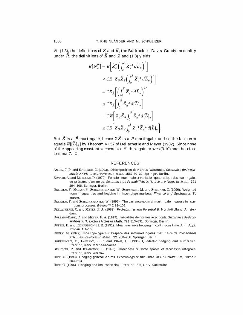
1830 T. RHEINLANDER AND M. SCHWEIZER
N, (1.3), the definitions of Z and R, the Burkholder–Davis–Gundy inequalityunder R, the definitions of R and Z and (1.3) yields
E[N2S
] = E
[Z2S
(∫ S0Z−1u dLu
)2]
≤ CE[ZSZS
(∫ S0Z−1u dLu
)2]
= CER
[(∫ S0Z−1u dLu
)2]
≤ CER
[∫ S0Z−2u dL�u
]
= CE
[ZSZS
∫ S0Z−2u dL�u
]
≤ CE[ZSZS
∫ S0Z−1u Z
−1u dL�u
]�
But Z is a P-martingale, hence ZZ is a P-martingale, and so the last termequals EL�S� by Theorem VI.57 of Dellacherie and Meyer (1982). Since noneof the appearing constants depends on S, this again proves (3.10) and thereforeLemma 7. ✷
REFERENCES
Ansel, J. P. and Stricker, C. (1993). Decomposition de Kunita–Watanabe. Seminaire de Proba-bilites XXVII. Lecture Notes in Math. 1557 30–32. Springer, Berlin.
Bonami, A. and Lepingle, D. (1979). Fonction maximale et variation quadratique des martingalesen presence d’un poids. Seminaire de Probabilites XIII. Lecture Notes in Math. 721294–306. Springer, Berlin.
Delbaen, F., Monat, P., Schachermayer, W., Schweizer, M. and Stricker, C. (1996). Weightednorm inequalities and hedging in incomplete markets. Finance and Stochastics. Toappear.
Delbaen, F. and Schachermayer, W. (1996). The variance-optimal martingale measure for con-tinuous processes. Bernoulli 2 81–105.
Dellacherie, C. and Meyer, P. A. (1982). Probabilities and Potential B. North-Holland, Amster-dam.
Doleans-Dade, C. and Meyer, P. A. (1979). Inegalites de normes avec poids. Seminaire de Prob-abilites XIII. Lecture Notes in Math. 721 313–331. Springer, Berlin.
Duffie, D. and Richardson, H. R. (1991). Mean-variance hedging in continuous time. Ann. Appl.Probab. 1 1–15.
Emery, M. (1979). Une topologie sur l’espace des semimartingales. Seminaire de ProbabilitesXIII. Lecture Notes in Math. 721 260–280. Springer, Berlin.
Gourieroux, C., Laurent, J. P. and Pham, H. (1996). Quadratic hedging and numeraire.Preprint, Univ. Marne-la-Vallee.
Grandits, P. and Krawczyk, L. (1996). Closedness of some spaces of stochastic integrals.Preprint, Univ. Warsaw.
Hipp, C. (1993). Hedging general claims. Proceedings of the Third AFIR Colloquium, Rome 2603–613.
Hipp, C. (1996). Hedging and insurance risk. Preprint 1/96, Univ. Karlsruhe.
L2-PROJECTIONS ON STOCHASTIC INTEGRALS 1831
Memin, J. (1980). Espaces de semimartingales et changement de probabilite. Zeit. Wahrsch. Verw.Gebiete 52 9–39.
Pham, H., Rheinlander, T. and Schweizer, M. (1996). Mean-variance hedging for continuousprocesses: new proofs and examples. Finance and Stochastics. To appear.
Protter, P. (1990). Stochastic Integration and Differential Equations. A New Approach. Springer,New York.
Schweizer, M. (1994). Approximating random variables by stochastic integrals. Ann. Probab. 221536–1575.
Schweizer, M. (1995a). On the minimal martingale measure and the Follmer–Schweizer decom-position. Stochastic Anal. Appl. 13 573–599.
Schweizer, M. (1995b). Variance-optimal hedging in discrete time. Math. Oper. Res. 20 1–32.Schweizer, M. (1996). Approximation pricing and the variance-optimal martingale measure.
Ann. Probab. 24 206–236.Wiese, A. (1995). Hedging stochastischer Verpflichtungen. In Workshop on Discrete Stochas-
tic Models (P. Eichelsbacher and M. Lowe, eds.) 28–32. Univ. Bielefeld, SFB 343Erganzungsreihe 95-002.
Technische Universitat BerlinFachbereich Mathematik, MA 7-4Straße des 17. Juni 136D-10623 BerlinGermanyE-mail: [email protected]