Inter J Nav Archit Oc Engng (2011) 3:274~285 http://dx.doi.org./10.2478/IJNAOE-2013-0071

SNAK, 2011

Buckling analysis and optimal structural design of supercavitating vehicles using finite element technology

Wanil Byun1, Min Ki Kim1, Kook Jin Park1, Seung Jo Kim1, Minho Chung2, Jin Yeon Cho2 and Sung-Han Park3

1School of Aerospace and Mechanical Engineering, Seoul National University, Seoul, Korea 2Department of Aerospace Engineering, Inha University, Incheon, Korea

3Agency for Defence Development, Deajeon, Korea

ABSTRACT: The supercavitating vehicle is an underwater vehicle that is surrounded almost completely by a supercavity to reduce hydrodynamic drag substantially. Since the cruise speed of the vehicle is much higher than that of conventional submarines, the drag force is huge and a buckling may occur. The buckling phenomenon is analyzed in this study through static and dynamic approaches. Critical buckling load and pressure as well as buckling mode shapes are calculated using static buckling analysis and a stability map is obtained from dynamic buckling analysis. When the finite element method (FEM) is used for the buckling analysis, the solver requires a linear static solver and an eigenvalue solver. In this study, these two solvers are integrated and a consolidated buckling analysis module is constructed. Furthermore, Particle Swarm Optimization (PSO) algorithm is combined in the buckling analysis module to perform a design optimization computation of a simplified supercavitating vehicle. The simplified configuration includes cylindrical shell structure with three stiffeners. The target for the design optimization process is to minimize total weight while maintaining the given structure buckling-free.

KEY WORDS: Supercavitating vehicle; FEM, Static/dynamic buckling analysis; PSO (Particle Swarm Optimization) algorithm. INTRODUCTION

Supercavitation is a technology that uses cavitation effect

to create large gas bubble inside a liquid, allowing an object to travel at a great speed through the liquid by being wholly enveloped by the bubble. Supercavitating vehicle is currently studied most vividly for the military applications such as torpedoes and submarines. Many of the previous studies on guidance, control and stability have considered supercavitating vehicles as rigid bodies (Rand, 1997; Vasin, 2001; Kirschner, 2002). However, assumption of non-rigid body was introduced recently using a higher fidelity finite element model based on shell elements (Ruzzene, 2004). In supercavitating vehicles, the interaction between the water and the cavitator nose is particularly important as the drag force increases with the square of the speed and the cruise speed of this type of vehicles are usually very high. The drag force compresses the body in axial direction which may result in buckling. Buckling clearly means a structural failure and therefore it has been been identified as one of the limiting factors that determine the operating speed of supercavitating vehicles (Vasin, 2001; Ruzzene, 2004). Buckling stability also needs to be addressed in order to evaluate safety limit

and the stability analysis should be considered as an effort to extend operating range of the supercavitating vehicles.

The goal of this paper is to investigate the static and dynamic buckling characteristics of supercavitating vehicles composed of shell elements using FEM. The maximum allowed drag force is identified from the static buckling analysis and a buckling stability map can be drawn by combining results of dynamic buckling analysis. These results offer a set of constraint conditions during a design optimization procedure for minimizing the required weight. To optimize the supercavitating vehicle’s body, static and dynamic buckling analysis modules are developed by integrating linear static and eigenvalue FE analysis software (IPSAP) with a Parallel Multifrontal Solver (Kim, 1999). The integrated module is further enhanced with an optimization tool, a Particle Swarm Optimization based algorithm, implemented inside (Yoon, 2011).

FINITE ELEMENT FORMULATION

Strain-displacement relationship

The total strain state in a shell (ε) is expressed as a

combination of linear (marked as l) and nonlinear components (nl).

Corresponding author: Seung Jo Kim e-mail: sjkim@snu.ac.kr.

Copyright © 2011 Society of Naval Architects of Korea. Production and hosting by ELSEVIER B.V. This is an open access article under the CC BY-NC 3.0 license

( http://creativecommons.org/licenses/by-nc/3.0/ ).

Inter J Nav Archit Oc Engng (2011) 3:274~285 275

)()( nll εεε += (1)

where ε is a vector describes the strain state in a shell, composed by normal strains (εx, εy) and a shear strain (γxy) as

Txyyx γεεε =.

Following Eq. (2) and Eq. (3) are the linear and nonlinear components of Eq. (1), respectively.

( )l

uxvy

u vy x

ε

⎧ ⎫∂⎪ ⎪

∂⎪ ⎪⎪ ⎪∂

= ⎨ ⎬∂⎪ ⎪

⎪ ⎪∂ ∂+⎪ ⎪

∂ ∂⎩ ⎭

(2)

2 2 2

2 2 2( )

12

12

nl

u v wx x x

u v wy y y

u u v v w wx y x y x y

ε

⎧ ⎫⎛ ⎞∂ ∂ ∂⎛ ⎞ ⎛ ⎞ ⎛ ⎞+ +⎪ ⎪⎜ ⎟⎜ ⎟ ⎜ ⎟ ⎜ ⎟⎜ ⎟∂ ∂ ∂⎝ ⎠ ⎝ ⎠ ⎝ ⎠⎪ ⎪⎝ ⎠⎪ ⎪

⎛ ⎞⎪ ⎪⎛ ⎞ ⎛ ⎞ ⎛ ⎞∂ ∂ ∂⎜ ⎟= + +⎨ ⎬⎜ ⎟ ⎜ ⎟ ⎜ ⎟⎜ ⎟∂ ∂ ∂⎝ ⎠ ⎝ ⎠ ⎝ ⎠⎪ ⎪⎝ ⎠⎪ ⎪∂ ∂ ∂ ∂ ∂ ∂⎪ ⎪+ +⎪ ⎪∂ ∂ ∂ ∂ ∂ ∂⎩ ⎭

(3)

Strain, potential and kinetic energy

The total elastic energy (Π ) for the shell is express as

VU +=Π (4)

where U is strain energy and V is potential energy. Similar to the strain state equation (Eq. (1)), U and V in Eq. (4) represent linear and nonlinear components of the strain, respectively. The total elastic energy can be written as follow.

( ) ( ) ( )

012

l T l T nl

V VC dV dVε ε σ εΠ = ⋅ ⋅ + ⋅∫ ∫ (5)

where V in Eq. (5) is the volume of the shell, C is constitutive matrix for the shell’s material. σ0 is the initial stress vector, composed by normal stresses (σ x, σ y) and a shear stress (τxy) corresponding to the applied buckling loads.

Meanwhile the shell kinetic energy is expressed as

( )2 2 212 V

T u v w dVρ= + +∫ (6)

where ρ is the density of the shell’s material. Stiffness, geometric stiffness and mass matrix

The strain energy, or the first term in the right hand side

of Eq. (5), can be expressed as

[ ] ( ) ( )1 12 2

Tl T ls

VU C dV Kε ε δ δ= ⋅ ⋅ =∫

(7)

where δ is nodal displacement vector and Ks is the stiffness matrix which is

[ ] [ ] [ ][ ] [ ] [ ][ ]T Ts

V VK B C B dV B C B J d d dξ η ς= =∫ ∫ (8)

In Eq. (8), B is an interpolation matrix obtained by imposing the considered set of shape functions and J is the determinant of the Jacobian matrix.

Geometric stiffness (Martin, 1966; Marcal, 1969; MacNeal, 1978) is the first order approximation of geometrically nonlinear behavior and it is particularly useful in the linearizing buckling problem. The terms in the geometric stiffness matrix for an element are linear functions of the components of stress in the element. The geometric stiffness matrix is obtained from the potential energy V due to initial stress and it is expressed in terms of initial stress vector 0σ and nonlinear strain vector ( )nlε . The potential energy of Eq. (5) can be rewritten as

( )0

12

TT nlg

VV dV Kσ ε δ δ⎡ ⎤= ⋅ = ⎣ ⎦∫ (9)

where Kg is the geometric stiffness matrix or the initial stress matrix which is modeled as

[ ] [ ][ ] [ ] [ ][ ]0 0T T

gV V

K G G dV G G J d d dσ σ ξ η ς⎡ ⎤ = =⎣ ⎦ ∫ ∫ (10)

The geometric stiffness matrix is one of major terms in the buckling analysis, and is composed of in-plane, bending, and transverse shear terms as follow.

[ ] [ ][ ]

[ ] [ ][ ]

[ ] [ ][ ]

[ ] [ ][ ]

0

0

3

1 0 1

3

2 0 2

12

12

Tg i a i e

Tb b b e

Ts b s e

Ts b s e

K G G h J dA

G G h J dA

hG G J dA

hG G J dA

σ

σ

σ

σ

⎡ ⎤ =⎣ ⎦

+

+

+

∫ ∫∫ ∫∫ ∫∫ ∫

(11)

where h is a thickness of shell and the other terms are as follows:

[ ] [ ] i b

u yw x

v x G Gw y

u x v yδ δ

−∂ ∂⎧ ⎫∂ ∂⎧ ⎫⎪ ⎪∂ ∂ = =⎨ ⎬ ⎨ ⎬∂ ∂⎩ ⎭⎪ ⎪∂ ∂ −∂ ∂⎩ ⎭

[ ] [ ] 1 2yx

s syx

xxG G

yyθθ

δ δθθ∂ ∂∂ ∂ ⎧ ⎫⎧ ⎫ ⎪ ⎪= =⎨ ⎬ ⎨ ⎬∂ ∂∂ ∂ ⎪ ⎪⎩ ⎭ ⎩ ⎭

(12)

276 Inter J Nav Archit Oc Engng (2011) 3:274~285

[ ]0

0 20 2

2 2 0

y xy

a x xy

xy xy

σ τσ σ τ

τ τ

⎡ ⎤−⎢ ⎥= −⎢ ⎥⎢ ⎥− −⎣ ⎦

[ ] ⎥⎦

⎤⎢⎣

⎡=

yxy

xyxb στ

τσσ0

(13)

The calculations of gradients which compose G are

straightforward using isoparametic formulations. For example, xu ∂∂ is computed as

jj

j

Nu uy y

∂∂=

∂ ∂∑ (14)

where N is a shape function, and other gradients can be calculated similarly.

Lastly, the shell kinetic energy is modeled as

[ ] 12

TT Mδ δ=

(15)

M is the mass matrix, which is given by

[ ] [ ] [ ] [ ] [ ]T T

V VM N N dV N N J d d dρ ρ ξ η ς= =∫ ∫ (16)

Governing equation

The equation of motion, derived from Hamilton’s

principle, is expressed using nodal displacement vector ( δ ), its second derivative ( δ ), and the modeled global matrices such as stiffness (Ks), geometric stiffness (Kg) and mass (M) matrix.

[ ] [ ] 0s gM K Kδ δ⎡ ⎤⎡ ⎤+ + =⎣ ⎦⎣ ⎦ (17)

The equation of motion is firstly used to perform static

buckling analysis as follow:

[ ] 0s i gK Kλ δ⎡ ⎤⎡ ⎤+ =⎣ ⎦⎣ ⎦ (18)

where iλ is ith eigenvalue of this system. Eq. (18) is similar to a general eigenvalue problem of structures except that mass matrix is replaced by the geometric stiffness matrix. Therefore, critical buckling load, Fcr, and critical buckling pressure, Pcr, can be obtained through an eigenvalue solver with an initial loading condition (F or P).

,cr i cr iF F P Pλ λ= = (19)

Then, the critical velocity, Vcr, which determines

operation range of the supercavitating vehicle can be

obtained from critical buckling load or pressure as follow (Ahn, 2006).

cc Dcw

crcc

Dcw

crcr CAρ

PhRπCAρ

FV 42== (20)

where ρw is the density of the water, Ac is the cross-sectional area of the cavitator,

cDC is the drag coefficient of the cavitator disk and Rc, hc denote the mid-radius and thickness of the supercavitating vehicle. This critical buckling load or critical velocity is one of the constraint conditions in performing optimal structural design which will be discussed later in this paper.

The equation of motion (Eq. (17)) is also used for the dynamic buckling analysis. Consider a case where an axial force F is periodic in time with a frequency of Ω .

)Ωcos1(Ωcos)( 000 tβFtFFtF d +=+= (21)

where F0 is the constant component of the distributed axial force, while Fd0 define amplitude of the time-varying component. The magnitude Fd0 is expressed in terms F0 of through the ratio β = Fd0/ F0. β is called a dynamic load factor. With the force given as Eq. (21), the equation of motion (Eq. (17)) can be rewritten as

[ ] [ ] ( ) 1 cos 0s gM K t Kδ β δ⎡ ⎤⎡ ⎤+ + + Ω =⎣ ⎦⎣ ⎦ (22)

Eq. (22) represents a system of second order differential

equation with a periodic coefficient, which is basically the Mathieu-Hill equation. The boundaries of instability region can be found by having periods of T and 2T where

Ω/2πT = . The instability regions for various combinations of the axial force parameters can be drawn using Bolotin’s method (Bolotin, 1964). The force variation defined in Eq. (21) describes a case of parametric excitation that causes instability when load frequency and the natural frequencies of the structure ( ω ) are in particular relationships. The amplitude of the load is assumed to be sufficiently small so that parametric resonance is achieved for frequencies of

kωi /2Ω = with any integer k. For practical purposes, the most important and dangerous parametric excitation conditions occur when k is unity. These frequency values are denoted as principal parametric resonances. According to the Bolotin’s method, a first approximation for the boundaries of the stability regions that corresponding to the principal parametric resonances are obtained by imposing in Eq. (22) periodic solutions of the kind:

( ) sin cos2 2t tt A Bδ Ω Ω

= + (23)

where A, B are arbitrary vectors. Plugging Eq. (23) into Eq. (22) and further manipulating the terms, a set of linear algebraic equations is obtained. The condition for non-trivial

Inter J Nav Archit Oc Engng (2011) 3:274~285 277

solutions, i.e. for an unstable response of the system, is given by

[ ] [ ]211 0

2 4s gK K Mβ Ω⎛ ⎞ ⎡ ⎤+ ± − =⎜ ⎟ ⎣ ⎦⎝ ⎠ (24)

Two frequencies corresponding to the plus and minus

sign in front of β21

in Eq. (24) determine the boundaries of

the dynamic instability map. Lower boundary of the instability region is calculated with plus sign while upper boundary is related to the minus sign.

Buckling analysis procedure

Steps for analyzing a buckling problem that includes

geometric stiffness matrix construction are as follow (MacNeal, 1972): Step 1. Solve a linear static response problem that does not

include geometric stiffness, and compute initial stress in each element.

Step 2. Calculate geometric stiffness matrix for individual

elements using the results of Step 1, and further compute geometric stiffness matrix Kg in Eq. (11).

Step 3a (for a static buckling problem). Find eigenvalues

and eigenvectors from Eq. (18). Critical buckling loads are the multiplications of the applied static loading with the eigenvalues calculated in this step.

Step 3b (for a dynamic buckling problem). Find eigenvalues

for Eq. (24) which determine lower (frequency

obtained with ‘+’ sign in front of β21 ) and upper

(with ‘–’ sign) boundaries of the stability map.

OPTIMIZATION ALGORITHM

Particle Swarm Optimization (PSO) algorithm Optimization has been one of the most frequently facing

issues in engineering field. Lately, numerical approach is commonly used for optimizing a variety of NP-complete problems such as structural optimization, neural network training, control system analysis and design. Efficiency of most numerical optimization methods is limited by two major obstacles. Firstly, even medium-scale problems can be computationally demanding due to the costly fitness evaluation step. Secondly, since most engineering optimization problems have multiple local optima, the use of global search methods is required such as population-based algorithms to deliver reliable results. The Particle Swarm Optimization (PSO) algorithm is an alternative choice to overcome the listed obstacles. It is a population-based skill

similar to the genetic algorithm, but rather a stochastic global optimization technique (Eberhart, 1995) and this method bases on the social behavior metaphor. The PSO algorithm is gaining attention as a non-gradient based global optimization method suited to continuous variable problems with successful applications to large-scale engineering optimization problems (Venter, 2002; Schutte, 2004).

In the PSO algorithm, the number of particles are randomly distributed in the domain and the particle group is called as swarm. Each particle is updated with the following equations (Eq. (25) and (26)) that are written in vector notation. Velocity of the ith particle is updated from kth to k+1th iteration as (Eq. (25))

( ) ( )k

ikg

ki

ki

ki

ki xprcxprcavv −+−+=+

22111 (25) The first term on the right hand side indicates that a

momentum factor a determines the amount of contribution of velocity at kth iteration to the next step. Next two terms on the right hand side attract the particle toward two best positions, pi

k and pg

k. pik is the previous best position of ith

particle and pgk

is the best position among all particles in

the swarm up to the kth iteration. The best position means the position at which the particle’s fitness value (f(pg

k)) is lower than any other fitness value that has been searched thus far. The strengths of the attractions are given by the coefficients c1 and c2. r1 and r2 are uniformly distributed random numbers between 0 and 1.

Using the velocity obtained vi k+1, position of the particle i is updated from the current position xi

k to the next xi

k+1 as

follow with coefficients c and d.

11 ++ += ki

ki

ki dvcxx (26)

The updating procedure is repeated until either a specified

convergence tolerance or predetermined total generation number is reached.

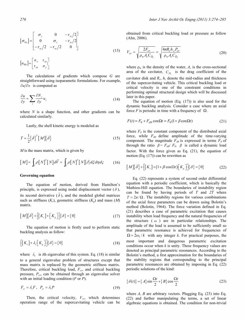
Fig. 1 Position and velocity update of particle. For instance, consider a simplified exampled in Fig. 1

with a swarm consists of seven particles. Updating velocity

278 Inter J Nav Archit Oc Engng (2011) 3:274~285

and position of the particle No. 2 requires to know the values at kth iteration (v2

k, x2k), the best position of this particle at the

previous iterations (p2k, assumed at the upper part in the

figure), and the global best position at kth iteration (pgk,

assumed at the third particle location). The effects of the coefficients are depicted as arrows in the figure.

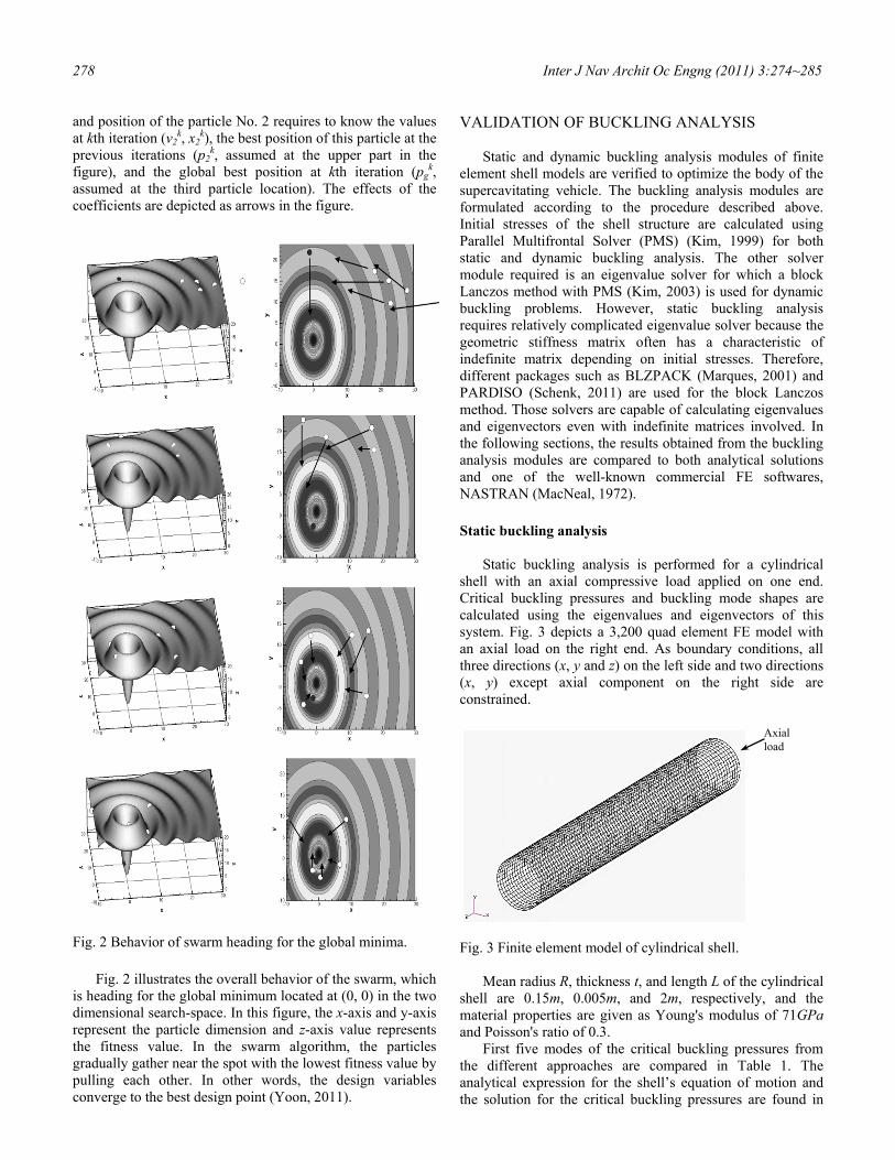
Fig. 2 Behavior of swarm heading for the global minima.

Fig. 2 illustrates the overall behavior of the swarm, which is heading for the global minimum located at (0, 0) in the two dimensional search-space. In this figure, the x-axis and y-axis represent the particle dimension and z-axis value represents the fitness value. In the swarm algorithm, the particles gradually gather near the spot with the lowest fitness value by pulling each other. In other words, the design variables converge to the best design point (Yoon, 2011).

VALIDATION OF BUCKLING ANALYSIS Static and dynamic buckling analysis modules of finite

element shell models are verified to optimize the body of the supercavitating vehicle. The buckling analysis modules are formulated according to the procedure described above. Initial stresses of the shell structure are calculated using Parallel Multifrontal Solver (PMS) (Kim, 1999) for both static and dynamic buckling analysis. The other solver module required is an eigenvalue solver for which a block Lanczos method with PMS (Kim, 2003) is used for dynamic buckling problems. However, static buckling analysis requires relatively complicated eigenvalue solver because the geometric stiffness matrix often has a characteristic of indefinite matrix depending on initial stresses. Therefore, different packages such as BLZPACK (Marques, 2001) and PARDISO (Schenk, 2011) are used for the block Lanczos method. Those solvers are capable of calculating eigenvalues and eigenvectors even with indefinite matrices involved. In the following sections, the results obtained from the buckling analysis modules are compared to both analytical solutions and one of the well-known commercial FE softwares, NASTRAN (MacNeal, 1972).

Static buckling analysis

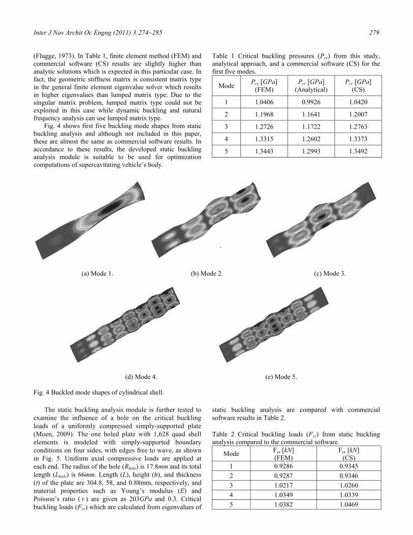
Static buckling analysis is performed for a cylindrical

shell with an axial compressive load applied on one end. Critical buckling pressures and buckling mode shapes are calculated using the eigenvalues and eigenvectors of this system. Fig. 3 depicts a 3,200 quad element FE model with an axial load on the right end. As boundary conditions, all three directions (x, y and z) on the left side and two directions (x, y) except axial component on the right side are constrained.

Fig. 3 Finite element model of cylindrical shell. Mean radius R, thickness t, and length L of the cylindrical

shell are 0.15m, 0.005m, and 2m, respectively, and the material properties are given as Young's modulus of 71GPa and Poisson's ratio of 0.3.

First five modes of the critical buckling pressures from the different approaches are compared in Table 1. The analytical expression for the shell’s equation of motion and the solution for the critical buckling pressures are found in

Axial load

Inter J Nav Archit Oc Engng (2011) 3:274~285 279

(Flugge, 1973). In Table 1, finite element method (FEM) and commercial software (CS) results are slightly higher than analytic solutions which is expected in this particular case. In fact, the geometric stiffness matrix is consistent matrix type in the general finite element eigenvalue solver which results in higher eigenvalues than lumped matrix type. Due to the singular matrix problem, lumped matrix type could not be exploited in this case while dynamic buckling and natural frequency analysis can use lumped matrix type.

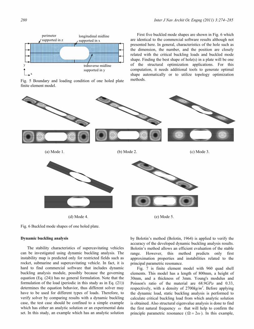
Fig. 4 shows first five buckling mode shapes from static buckling analysis and although not included in this paper, these are almost the same as commercial software results. In accordance to these results, the developed static buckling analysis module is suitable to be used for optimization computations of supercavitating vehicle’s body.

Table 1 Critical buckling pressures (Pcr) from this study, analytical approach, and a commercial software (CS) for the first five modes.

Mode Pcr [GPa] (FEM)

Pcr [GPa] (Analytical)

Pcr [GPa] (CS)

1 1.0406 0.9926 1.0420

2 1.1968 1.1641 1.2007

3 1.2726 1.1722 1.2763

4 1.3315 1.2602 1.3373

5 1.3443 1.2993 1.3492

(a) Mode 1. (b) Mode 2. (c) Mode 3.

(d) Mode 4. (e) Mode 5.

Fig. 4 Buckled mode shapes of cylindrical shell.

The static buckling analysis module is further tested to

examine the influence of a hole on the critical buckling loads of a uniformly compressed simply-supported plate (Moen, 2009). The one holed plate with 1,628 quad shell elements is modeled with simply-supported boundary conditions on four sides, with edges free to wave, as shown in Fig. 5. Uniform axial compressive loads are applied at each end. The radius of the hole (Rhole) is 17.8mm and its total length (Lhole) is 66mm. Length (L), height (h), and thickness (t) of the plate are 304.8, 58, and 0.88mm, respectively, and material properties such as Young’s modulus (E) and Poisson’s ratio ( ν ) are given as 203GPa and 0.3. Critical buckling loads (Fcr) which are calculated from eigenvalues of

static buckling analysis are compared with commercial software results in Table 2. Table 2 Critical buckling loads (Fcr) from static buckling analysis compared to the commercial software.

Mode Fcr [kN] (FEM)

Fcr [kN] (CS)

1 0.9286 0.9345 2 0.9287 0.9346 3 1.0217 1.0260 4 1.0349 1.0339 5 1.0382 1.0469

280 Inter J Nav Archit Oc Engng (2011) 3:274~285

Fig. 5 Boundary and loading condition of one holed plate finite element model.

First five buckled mode shapes are shown in Fig. 6 which are identical to the commercial software results although not presented here. In general, characteristics of the hole such as the dimension, the number, and the position are closely related with the critical buckling loads and buckled mode shape. Finding the best shape of hole(s) in a plate will be one of the structural optimization applications. For this computation, it needs additional tools to generate optimal shape automatically or to utilize topology optimization methods.

(a) Mode 1.

(b) Mode 2.

(c) Mode 3.

(d) Mode 4.

(e) Mode 5.

Fig. 6 Buckled mode shapes of one holed plate.

Dynamic buckling analysis

The stability characteristics of supercavitating vehicles

can be investigated using dynamic buckling analysis. The instability map is predicted only for restricted fields such as rocket, submarine and supercavitating vehicle. In fact, it is hard to find commercial software that includes dynamic buckling analysis module, possibly because the governing equation (Eq. (24)) has no general formulation. Note that the formulation of the load (periodic in this study as in Eq. (21)) determines the equation behavior, thus different solver may have to be used for different types of loads. Therefore, to verify solver by comparing results with a dynamic buckling case, the test case should be confined to a simple example which has either an analytic solution or an experimental data set. In this study, an example which has an analytic solution

by Bolotin’s method (Bolotin, 1964) is applied to verify the accuracy of the developed dynamic buckling analysis results. Bolotin’s method allows an efficient evaluation of the stable range. However, this method predicts only first approximation properties and instabilities related to the principal parametric resonance.

Fig. 7 is finite element model with 960 quad shell elements. This model has a length of 800mm, a height of 30mm, and a thickness of 3mm. Young's modulus and Poisson's ratio of the material are 68.9GPa and 0.33, respectively, with a density of 2700kg/m3. Before applying the dynamic load, static buckling analysis is performed to calculate critical buckling load from which analytic solution is obtained. Also structural eigenvalue analysis is done to find the first natural frequency ω that will help to confirm the principle parametric resonance ( ω2Ω = ). In this example,

x

y

perimeter supported in z

transverse midline supported in y

longitudinal midline supported in x

Inter J Nav Archit Oc Engng (2011) 3:274~285 281

the critical buckling load is 71.73N and the first natural frequency is 10.74Hz.

Fig. 7 Simple FE shell model with a periodic loading.

Once including an axial force varying in time as in Eq.

(27), governing equation becomes Eq. (28).

tβFtF Ωcos)( 0= (27)

[ ] [ ]2

02 4s gK K Mβ Ω⎛ ⎞⎡ ⎤± − =⎜ ⎟⎣ ⎦⎝ ⎠

(28)

Applying Bolotin's method and set a unity dynamic load

factor β , it is possible to investigate unstable region for the given range of amplitude F0, 0 to 50N. Fig. 8 shows the stability map of which lower boundary (dashed line) is calculated with the positive sign in front of ( β /2) in Eq. (28) while upper boundary (solid line) is the solution when the sign associated with Kg term in Eq. (28) is negative. Unstable region belongs to the area between the two lines, and it is indicated that the unstable region is wider with larger amplitude force. In the figure, the two lines merge when the amplitude force diminishes and at this moment, the principle parametric resonance can confirm twice of the first natural frequency as discussed earlier. Table 3 compares the results plotted in Fig. 8 in numbers and they are very close to each other with the maximum difference less than 0.3%. The dynamic buckling analysis module developed in this study is fully validated through the presented test case.

Fig. 8 Stability map for simple shell.

Table 3 Boundaries of unstable region computed using finite element method compared to analytic solutions ( β =1.0).

Amplitudeof force

Analytical [Hz] FEM [Hz]

Lower Upper Lower Upper

0 21.48 21.48 21.48 21.48

10 20.73 22.23 20.71 22.22

20 19.94 22.94 19.91 22.93

30 19.12 23.63 19.09 23.62

40 18.26 24.30 18.23 24.30

50 17.35 24.95 17.30 24.95 OPTIMAL DESIGN OF SUPERCAVITATING VEHICLE’S STRUCTURE

Underwater supercavitating vehicles can be approximated

as slender elastic bodies, and thus in this study, the structural behavior is modeled using the shell finite element formulation. The nature of the forces acting on supercavitating vehicles is very complex and still under extensive experimental and numerical investigations. The results presented in this study are intended to provide design guidelines which will help estimating the critical buckling loads, buckled mode shapes, stability map and their optimal design for the considered type of vehicles. In addition, the optimal design procedure with minimizing weight using static and dynamic buckling has a great potential in that it can be extended to other structures such as rockets, , and submarines.

Overview At the cruise speed, as depicted in Fig. 9, the

supercavitating vehicle interacts with the liquid phase through its front surface (cavitator) and a cavity that surrounds most parts of the vehicle. The ellipse around the vehicle in the figure represents the cavity boundary.

Fig. 9 Schematic of forces applied on the supercavitating vehicle moving with a velocity V.

For the purpose of the buckling analysis, the vehicle’s

interactions with the fluid can be simplified as a combination of a distributed axial force, corresponding to the drag at the nose and to the propulsion at the tail. The drag force FD experienced by the vehicle during its forward motion is given by Eq. (29) (Vasin, 2001; Kirschner, 2001).

V

FDFP

282 Inter J Nav Archit Oc Engng (2011) 3:274~285

2

21 VCAρF

cDcwD = (29)

where wρ is the density of the water, Ac is the cross-sectional area of the cavitator,

cDC is the drag coefficient of the cavitator disk, and V is the velocity of the vehicle. The drag coefficient for a cavitator disk can be expressed as Eq. (30) with an angle of attack cα (Kirschner, 2002).

( )

2

2

21;cos)1(

0

Vρ

ppσασCCw

ccDDc

−=+= ∞ (30)

where

0DC is the cavitator drag coefficient without any angle of attack which is chosen as 0.805 (Kirschner, 2002) and σ is the cavitation number. In this study, the area of the initial designed cavitator (Ac) is set to 0.00942 m2 that corresponds to a circular disc of a radius Rc=0.15m. Other flow parameters are chosen reasonably; for example, the water density ( wρ ) is 1000kg/m3, the ambient pressure ( ∞p ) is 98.1kPa which corresponds to 10m depth of water, and the cavity pressure ( cp ) is 2.5kPa, a typical value for gaseous cavities (Ahn, 2006).

In normal operating conditions, the total drag force FD is equilibrated by the propulsion force FP. Drag and propulsion forces are applied to the shell structure as axial forces distributed along the circumferential cross section of the shell.

In the static buckling analysis case, a critical buckling load, i.e. a maximum drag force which is safe from buckling phenomena, can be predicted by Eq. (18) and Eq. (19). In the dynamic buckling analysis, the axial force F(t) is represented as the sum of a constant component and a time varying term which accounts for the oscillatory force applied to the structure. If the considered axial force of the supercavitating vehicle is in the form of Eq. (21), the governing equation becomes Eq. (24) in this cavitator problem.

Fig. 10 is a finite element model of simplified supercavitating vehicle with stiffeners. Mean radius (Rc), thickness (hc), and length (L) of this model are 0.15, 0.01, and 2m, respectively, and the Young's modulus (E), Poisson's ratio (ν), and density (ρ) of the material are 71GPa, 0.3, and 2700kg/ m3.

Fig. 10 Finite element shell model of simplified supercavitating vehicle with stiffeners.

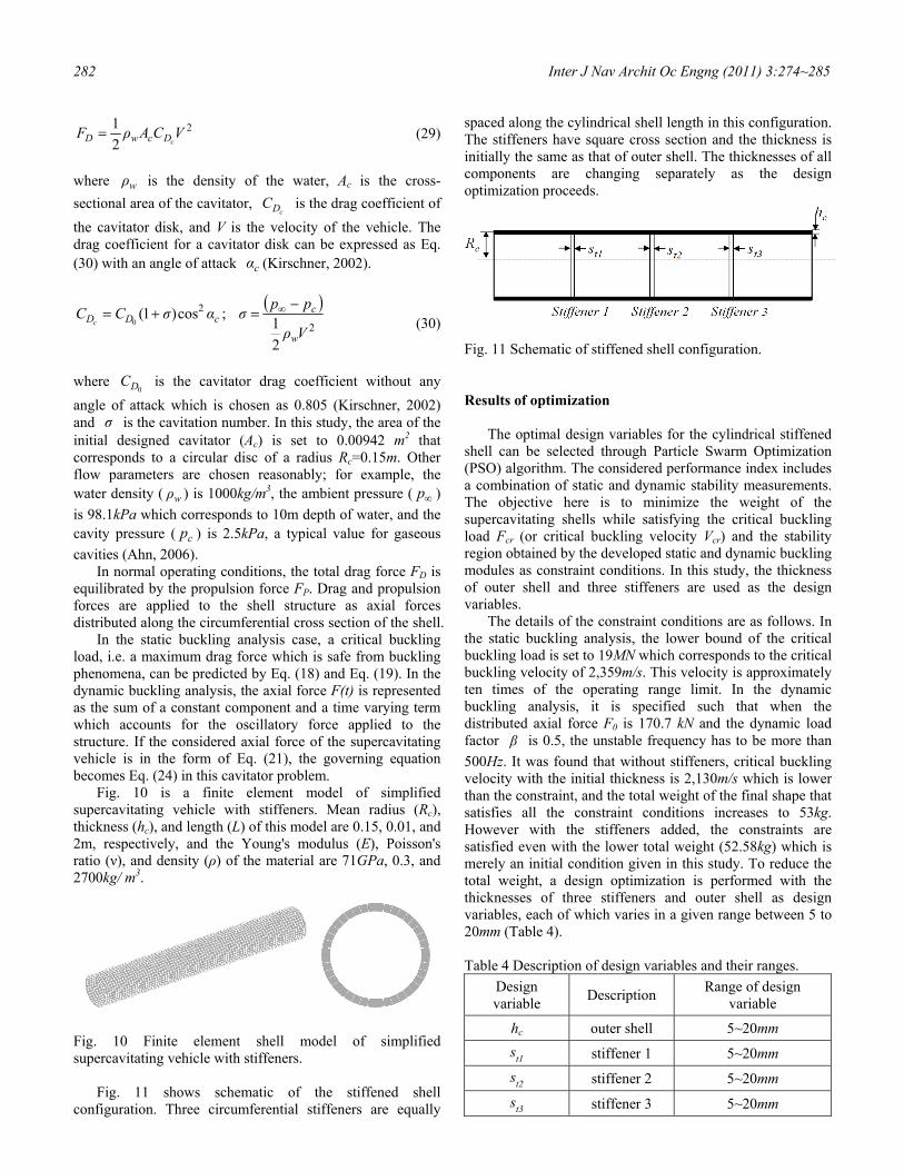
Fig. 11 shows schematic of the stiffened shell

configuration. Three circumferential stiffeners are equally

spaced along the cylindrical shell length in this configuration. The stiffeners have square cross section and the thickness is initially the same as that of outer shell. The thicknesses of all components are changing separately as the design optimization proceeds.

Fig. 11 Schematic of stiffened shell configuration.

Results of optimization The optimal design variables for the cylindrical stiffened

shell can be selected through Particle Swarm Optimization (PSO) algorithm. The considered performance index includes a combination of static and dynamic stability measurements. The objective here is to minimize the weight of the supercavitating shells while satisfying the critical buckling load Fcr (or critical buckling velocity Vcr) and the stability region obtained by the developed static and dynamic buckling modules as constraint conditions. In this study, the thickness of outer shell and three stiffeners are used as the design variables.

The details of the constraint conditions are as follows. In the static buckling analysis, the lower bound of the critical buckling load is set to 19MN which corresponds to the critical buckling velocity of 2,359m/s. This velocity is approximately ten times of the operating range limit. In the dynamic buckling analysis, it is specified such that when the distributed axial force F0 is 170.7 kN and the dynamic load factor β is 0.5, the unstable frequency has to be more than 500Hz. It was found that without stiffeners, critical buckling velocity with the initial thickness is 2,130m/s which is lower than the constraint, and the total weight of the final shape that satisfies all the constraint conditions increases to 53kg. However with the stiffeners added, the constraints are satisfied even with the lower total weight (52.58kg) which is merely an initial condition given in this study. To reduce the total weight, a design optimization is performed with the thicknesses of three stiffeners and outer shell as design variables, each of which varies in a given range between 5 to 20mm (Table 4).

Table 4 Description of design variables and their ranges.

Design variable Description Range of design

variable

hc outer shell 5~20mm st1 stiffener 1 5~20mm st2 stiffener 2 5~20mm st3 stiffener 3 5~20mm

Inter J Nav Archit Oc Engng (2011) 3:274~285 283

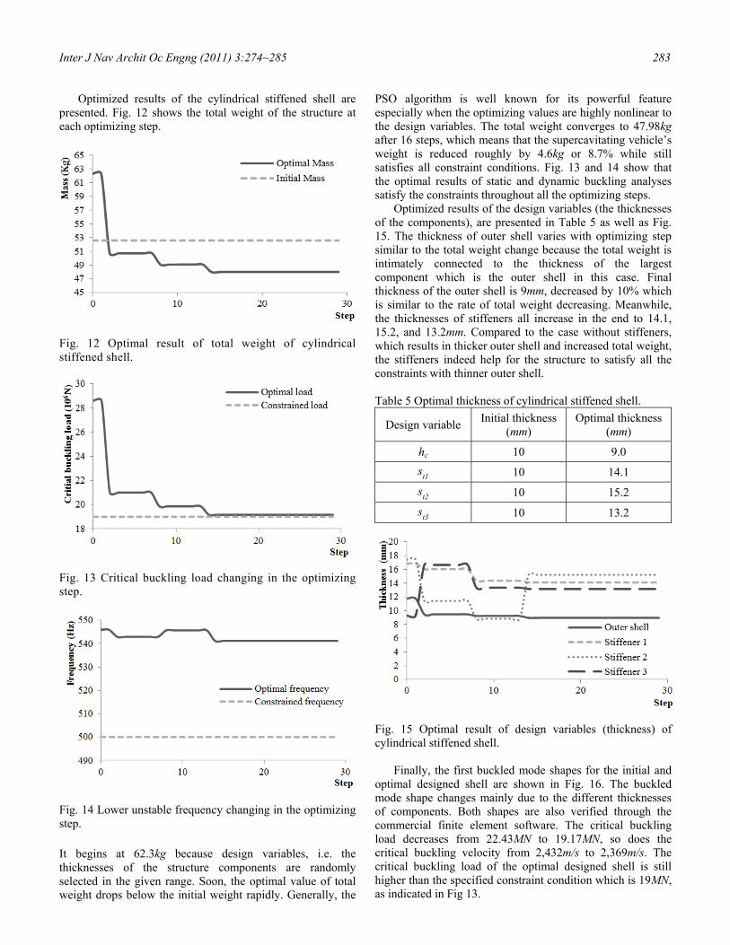
Optimized results of the cylindrical stiffened shell are presented. Fig. 12 shows the total weight of the structure at each optimizing step.

Fig. 12 Optimal result of total weight of cylindrical stiffened shell.

Fig. 13 Critical buckling load changing in the optimizing step.

Fig. 14 Lower unstable frequency changing in the optimizing step.

It begins at 62.3kg because design variables, i.e. the thicknesses of the structure components are randomly selected in the given range. Soon, the optimal value of total weight drops below the initial weight rapidly. Generally, the

PSO algorithm is well known for its powerful feature especially when the optimizing values are highly nonlinear to the design variables. The total weight converges to 47.98kg after 16 steps, which means that the supercavitating vehicle’s weight is reduced roughly by 4.6kg or 8.7% while still satisfies all constraint conditions. Fig. 13 and 14 show that the optimal results of static and dynamic buckling analyses satisfy the constraints throughout all the optimizing steps.

Optimized results of the design variables (the thicknesses of the components), are presented in Table 5 as well as Fig. 15. The thickness of outer shell varies with optimizing step similar to the total weight change because the total weight is intimately connected to the thickness of the largest component which is the outer shell in this case. Final thickness of the outer shell is 9mm, decreased by 10% which is similar to the rate of total weight decreasing. Meanwhile, the thicknesses of stiffeners all increase in the end to 14.1, 15.2, and 13.2mm. Compared to the case without stiffeners, which results in thicker outer shell and increased total weight, the stiffeners indeed help for the structure to satisfy all the constraints with thinner outer shell.

Table 5 Optimal thickness of cylindrical stiffened shell.

Design variable Initial thickness (mm)

Optimal thickness(mm)

hc 10 9.0 st1 10 14.1 st2 10 15.2 st3 10 13.2

Fig. 15 Optimal result of design variables (thickness) of cylindrical stiffened shell.

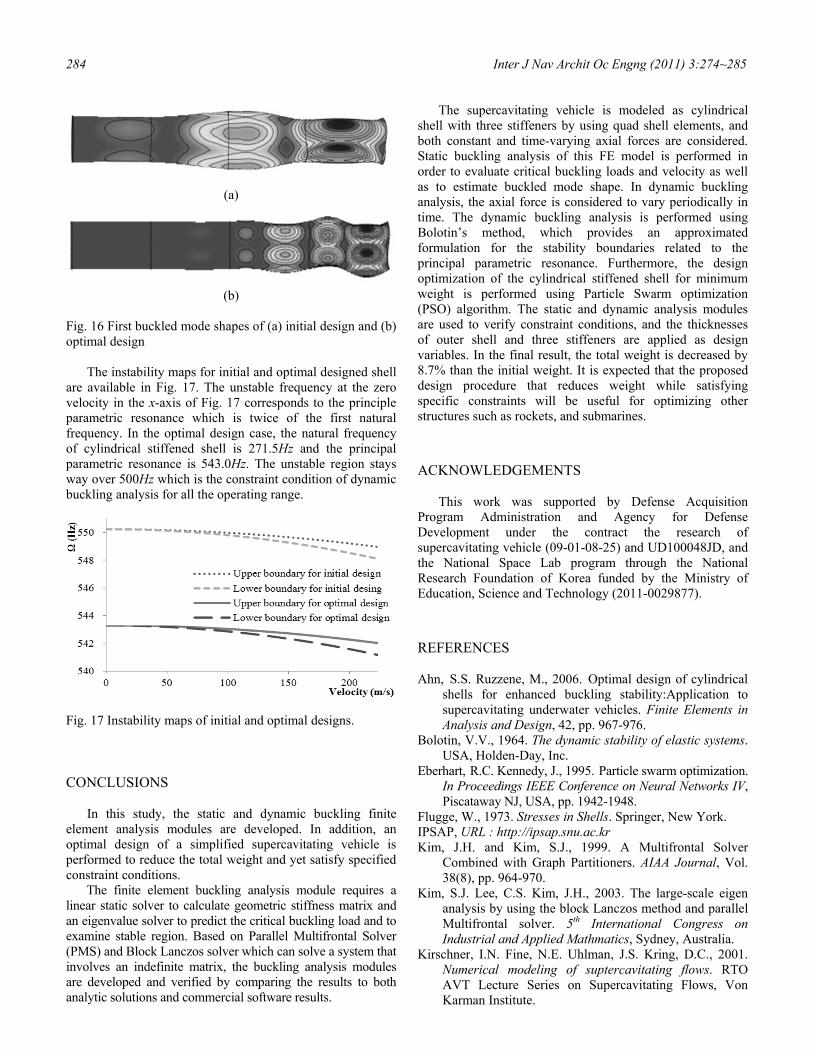
Finally, the first buckled mode shapes for the initial and

optimal designed shell are shown in Fig. 16. The buckled mode shape changes mainly due to the different thicknesses of components. Both shapes are also verified through the commercial finite element software. The critical buckling load decreases from 22.43MN to 19.17MN, so does the critical buckling velocity from 2,432m/s to 2,369m/s. The critical buckling load of the optimal designed shell is still higher than the specified constraint condition which is 19MN, as indicated in Fig 13.

284 Inter J Nav Archit Oc Engng (2011) 3:274~285

(a)

(b)

Fig. 16 First buckled mode shapes of (a) initial design and (b) optimal design

The instability maps for initial and optimal designed shell are available in Fig. 17. The unstable frequency at the zero velocity in the x-axis of Fig. 17 corresponds to the principle parametric resonance which is twice of the first natural frequency. In the optimal design case, the natural frequency of cylindrical stiffened shell is 271.5Hz and the principal parametric resonance is 543.0Hz. The unstable region stays way over 500Hz which is the constraint condition of dynamic buckling analysis for all the operating range.

Fig. 17 Instability maps of initial and optimal designs.

CONCLUSIONS In this study, the static and dynamic buckling finite

element analysis modules are developed. In addition, an optimal design of a simplified supercavitating vehicle is performed to reduce the total weight and yet satisfy specified constraint conditions.

The finite element buckling analysis module requires a linear static solver to calculate geometric stiffness matrix and an eigenvalue solver to predict the critical buckling load and to examine stable region. Based on Parallel Multifrontal Solver (PMS) and Block Lanczos solver which can solve a system that involves an indefinite matrix, the buckling analysis modules are developed and verified by comparing the results to both analytic solutions and commercial software results.

The supercavitating vehicle is modeled as cylindrical shell with three stiffeners by using quad shell elements, and both constant and time-varying axial forces are considered. Static buckling analysis of this FE model is performed in order to evaluate critical buckling loads and velocity as well as to estimate buckled mode shape. In dynamic buckling analysis, the axial force is considered to vary periodically in time. The dynamic buckling analysis is performed using Bolotin’s method, which provides an approximated formulation for the stability boundaries related to the principal parametric resonance. Furthermore, the design optimization of the cylindrical stiffened shell for minimum weight is performed using Particle Swarm optimization (PSO) algorithm. The static and dynamic analysis modules are used to verify constraint conditions, and the thicknesses of outer shell and three stiffeners are applied as design variables. In the final result, the total weight is decreased by 8.7% than the initial weight. It is expected that the proposed design procedure that reduces weight while satisfying specific constraints will be useful for optimizing other structures such as rockets, and submarines.

ACKNOWLEDGEMENTS

This work was supported by Defense Acquisition

Program Administration and Agency for Defense Development under the contract the research of supercavitating vehicle (09-01-08-25) and UD100048JD, and the National Space Lab program through the National Research Foundation of Korea funded by the Ministry of Education, Science and Technology (2011-0029877).

REFERENCES

Ahn, S.S. Ruzzene, M., 2006. Optimal design of cylindrical

shells for enhanced buckling stability:Application to supercavitating underwater vehicles. Finite Elements in Analysis and Design, 42, pp. 967-976.

Bolotin, V.V., 1964. The dynamic stability of elastic systems. USA, Holden-Day, Inc.

Eberhart, R.C. Kennedy, J., 1995. Particle swarm optimization. In Proceedings IEEE Conference on Neural Networks IV, Piscataway NJ, USA, pp. 1942-1948.

Flugge, W., 1973. Stresses in Shells. Springer, New York. IPSAP, URL : http://ipsap.snu.ac.kr Kim, J.H. and Kim, S.J., 1999. A Multifrontal Solver

Combined with Graph Partitioners. AIAA Journal, Vol. 38(8), pp. 964-970.

Kim, S.J. Lee, C.S. Kim, J.H., 2003. The large-scale eigen analysis by using the block Lanczos method and parallel Multifrontal solver. 5th International Congress on Industrial and Applied Mathmatics, Sydney, Australia.

Kirschner, I.N. Fine, N.E. Uhlman, J.S. Kring, D.C., 2001. Numerical modeling of suptercavitating flows. RTO AVT Lecture Series on Supercavitating Flows, Von Karman Institute.

Inter J Nav Archit Oc Engng (2011) 3:274~285 285

Kirschner, I.N. Kring, D.C. Stokes, A.W. Fine, N.E. and Uhlman, J.S., 2002. Control strategies for supercavitating vehicles. Journal of Vibration and Control, 8, pp. 219-242.

MacNeal, R.H., 1972. NASTRAN Theoretical manual. The MacNeal-Schwendler Corp.

MacNeal, R.H., 1978. A simple quadrilateral shell element. Computers & Structures, 8, pp. 175-183.

Marcal, P.V., 1969. Finite element analysis of combined problems of material and geometric behavior. Proc. Am. Soc. Mech. Eng. Conf. on Computational Approaches in Applied Mechanics, pp. 133.

Marques, O., 2001. BLZPACK User’s Guide. Martin, H.C., 1966. On the derivation of stiffness matrices for

the analysis of large deflection and stability problems. University of Washington, Department of Aeronautics and Astronautics, Roport 66-4.

Moen, C.D. Schafer, B.W., 2009. Elastic buckling of thin plates with holes in compression or bending. Thin-Walled Structures, Vol.47, pp. 1597-1607.

Rand, R. Pratap, R. Ramani, D. Cipolla, J. and Kirschner, I., 1997. Impact dynamics of a supercavitating underwater projectile. Proceedings of ASME Design Engineering Technical Conferences (DETC), Sacramento CA, USA.

Ruzzene, M., 2004. Dynamic buckling of periodically stiffened shells: application to supercavitating vechiles. International Journal of Solids and Structures, 41, pp. 1039-1059.

Ruzzene, M., 2004. Non-axisymmetric buckling of stiffened supercaviting shells: static and dynamic analysis. Computers and Structures, 82, pp. 257-269.

Schenk, O., Gartner, K., 2011. PARDISO : User Guide. Schutte, J.F. Reinbolt, J.A. Fregly, B.J. Haftka, R.T. and George,

A.D., 2004. Parallel global optimization with the particle swarm algorithm. International Journal for Numerical Methods in Engineering, 61(13), pp. 2296-2315.

Vasin, A.D., 2001. Some problems of supersonic cavitation flows. Proceedings of the 4th International Symposium on Cavitation, Pasadena CA, USA.

Venter, G. and Sobieszczanski-Sobieski, J., 2002. Multidisciplinary optimization of a transport aircraft wing using particle swarm optimization. 9th AIAA/ISSMO Symposium on Multidisciplinary Analysis and Optimization, Atlanta GA, USA.

Yoon, Y.H., 2011. Asynchronous particle swarm optimization with redistribution technique and its application to optimal design of satellite adapter-ring. Ph. D thesis, Seoul National University.