R7003E labs:state-space control of a balancing robot

Luleå University of Technology

Version 1.2.1

2016, LP2

xw

ywθw

xb

yb

θb

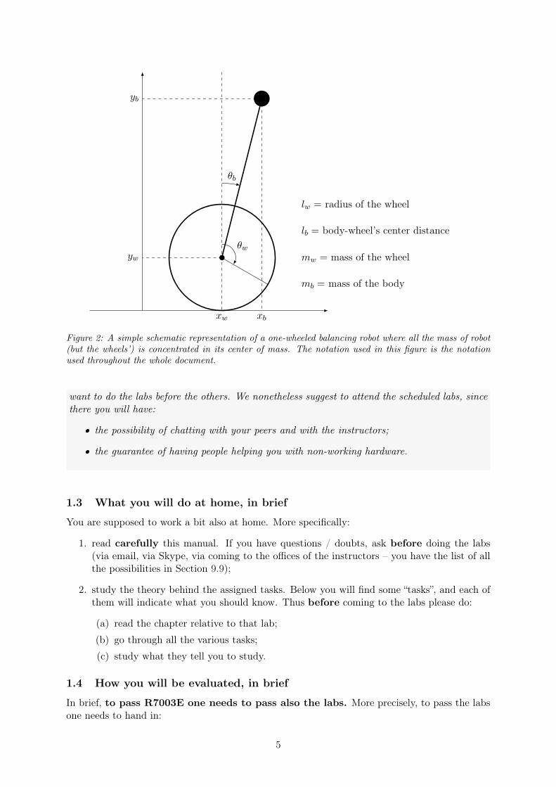
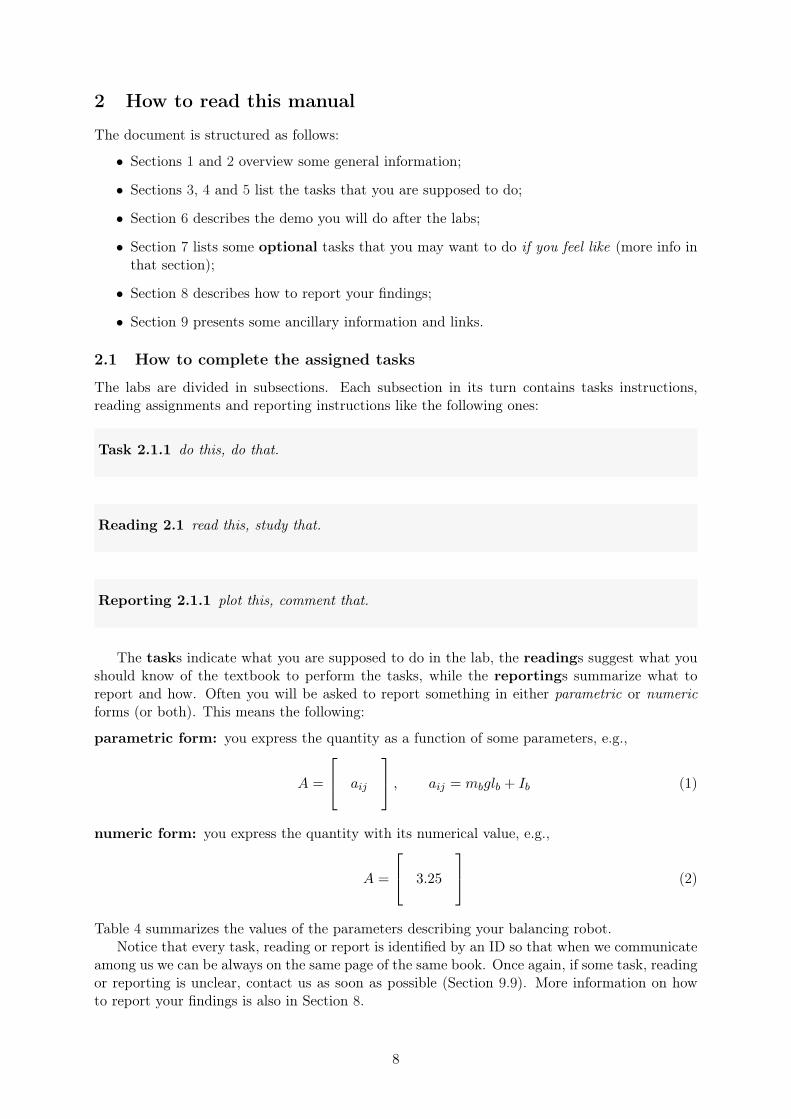
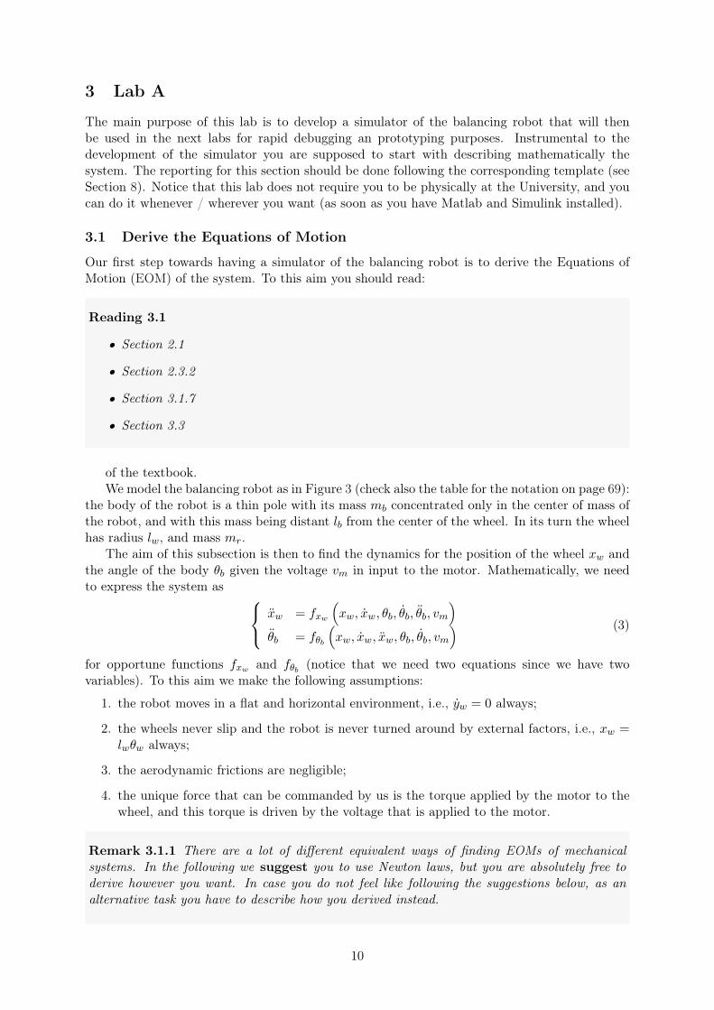
lw = radius of the wheel

lb = body-wheel’s center distance

mw = mass of the wheel

mb = mass of the body

Contents

1 What are the labs about 41.1 What a balancing robot is, and why it is an important system . . . . . . . . . . . 41.2 What you will do in the labs, in brief . . . . . . . . . . . . . . . . . . . . . . . . . 41.3 What you will do at home, in brief . . . . . . . . . . . . . . . . . . . . . . . . . . 51.4 How you will be evaluated, in brief . . . . . . . . . . . . . . . . . . . . . . . . . . 51.5 How we would like you to interact with your peers . . . . . . . . . . . . . . . . . 61.6 How we would like you to interact with us . . . . . . . . . . . . . . . . . . . . . . 6

2 How to read this manual 82.1 How to complete the assigned tasks . . . . . . . . . . . . . . . . . . . . . . . . . . 82.2 Notation . . . . . . . . . . . . . . . . . . . . . . . . . . . . . . . . . . . . . . . . . 9

3 Lab A 103.1 Derive the Equations of Motion . . . . . . . . . . . . . . . . . . . . . . . . . . . . 10

3.1.1 Dynamics of the wheel . . . . . . . . . . . . . . . . . . . . . . . . . . . . . 113.1.2 Dynamics of the body . . . . . . . . . . . . . . . . . . . . . . . . . . . . . 123.1.3 Dynamics of the motor . . . . . . . . . . . . . . . . . . . . . . . . . . . . . 15

3.2 Linearize the Equations of Motion . . . . . . . . . . . . . . . . . . . . . . . . . . 163.3 Write the linearized Equations of Motion in State-Space form . . . . . . . . . . . 173.4 Determine the transfer function relative to system (12) . . . . . . . . . . . . . . . 193.5 Design a PID controller stabilizing the transfer function computed in Section 3.4 203.6 Model the effect of disturbing the robot . . . . . . . . . . . . . . . . . . . . . . . 223.7 Check if everything is working as it should be . . . . . . . . . . . . . . . . . . . . 233.8 Convert the controller to the discrete domain . . . . . . . . . . . . . . . . . . . . 263.9 Simulate the closed loop system . . . . . . . . . . . . . . . . . . . . . . . . . . . . 273.10 (Optional) play with the simulator . . . . . . . . . . . . . . . . . . . . . . . . . . 31

4 Lab B 324.1 How to do tests on the robot . . . . . . . . . . . . . . . . . . . . . . . . . . . . . 324.2 Communicating with the balancing robot . . . . . . . . . . . . . . . . . . . . . . 334.3 Checking that reality is far from ideality . . . . . . . . . . . . . . . . . . . . . . . 354.4 Test the PID controller . . . . . . . . . . . . . . . . . . . . . . . . . . . . . . . . . 364.5 Check the controllability and observability properties of the linearized system (12) 384.6 Design a State-Space (SS) controller selecting the poles using a second order ap-

proximation . . . . . . . . . . . . . . . . . . . . . . . . . . . . . . . . . . . . . . . 394.7 Design a SS controller selecting the poles using the Linear-Quadratic Regulator

(LQR) technique . . . . . . . . . . . . . . . . . . . . . . . . . . . . . . . . . . . . 414.8 Design a state observer, and add it to the simulator . . . . . . . . . . . . . . . . . 434.9 Discretize both the controller and observer, and add them to the simulator . . . . 474.10 Test the control strategy with the real robot . . . . . . . . . . . . . . . . . . . . . 49

5 Lab C 515.1 Compute the discrete equivalent of the original model . . . . . . . . . . . . . . . 515.2 Design the controller using the discrete LQR technique . . . . . . . . . . . . . . . 515.3 Design the observer starting from the previously constructed controller . . . . . . 525.4 Perform experiments on the real balancing robot . . . . . . . . . . . . . . . . . . 535.5 Design a module for managing external references . . . . . . . . . . . . . . . . . . 54

2

6 Final demo 566.1 What it is . . . . . . . . . . . . . . . . . . . . . . . . . . . . . . . . . . . . . . . . 566.2 What you are supposed to do . . . . . . . . . . . . . . . . . . . . . . . . . . . . . 566.3 How you will be evaluated . . . . . . . . . . . . . . . . . . . . . . . . . . . . . . . 576.4 The R7003E 2016 LP2 International Balancing Robot Race . . . . . . . . . . . . 57

7 Optional tasks 59

8 Reporting your findings 608.1 The labs reports . . . . . . . . . . . . . . . . . . . . . . . . . . . . . . . . . . . . 60

8.1.1 What they are . . . . . . . . . . . . . . . . . . . . . . . . . . . . . . . . . 608.1.2 What you are supposed to do . . . . . . . . . . . . . . . . . . . . . . . . . 608.1.3 How you will be evaluated . . . . . . . . . . . . . . . . . . . . . . . . . . . 60

8.2 The final report . . . . . . . . . . . . . . . . . . . . . . . . . . . . . . . . . . . . . 618.2.1 What it is . . . . . . . . . . . . . . . . . . . . . . . . . . . . . . . . . . . . 618.2.2 What you are supposed to do . . . . . . . . . . . . . . . . . . . . . . . . . 618.2.3 How you will be evaluated . . . . . . . . . . . . . . . . . . . . . . . . . . . 61

8.3 Bonus points . . . . . . . . . . . . . . . . . . . . . . . . . . . . . . . . . . . . . . 61

9 Appendix 639.1 Installation in Windows . . . . . . . . . . . . . . . . . . . . . . . . . . . . . . . . 639.2 How to launch the code on the balancing robot . . . . . . . . . . . . . . . . . . . 639.3 How to plot data in Matlab / diagrams in Simulink . . . . . . . . . . . . . . . . . 639.4 Useful Simulink tricks . . . . . . . . . . . . . . . . . . . . . . . . . . . . . . . . . 649.5 Useful Simulink blocks . . . . . . . . . . . . . . . . . . . . . . . . . . . . . . . . . 649.6 Managing sampling times in Simulink . . . . . . . . . . . . . . . . . . . . . . . . 659.7 Useful Matlab commands . . . . . . . . . . . . . . . . . . . . . . . . . . . . . . . 659.8 Useful bash scripts . . . . . . . . . . . . . . . . . . . . . . . . . . . . . . . . . . . 659.9 Contacts . . . . . . . . . . . . . . . . . . . . . . . . . . . . . . . . . . . . . . . . . 669.10 List of the acronyms . . . . . . . . . . . . . . . . . . . . . . . . . . . . . . . . . . 669.11 Datasheet . . . . . . . . . . . . . . . . . . . . . . . . . . . . . . . . . . . . . . . . 689.12 Notation . . . . . . . . . . . . . . . . . . . . . . . . . . . . . . . . . . . . . . . . . 69

10 FAQ 69

3

1 What are the labs about

1.1 What a balancing robot is, and why it is an important system

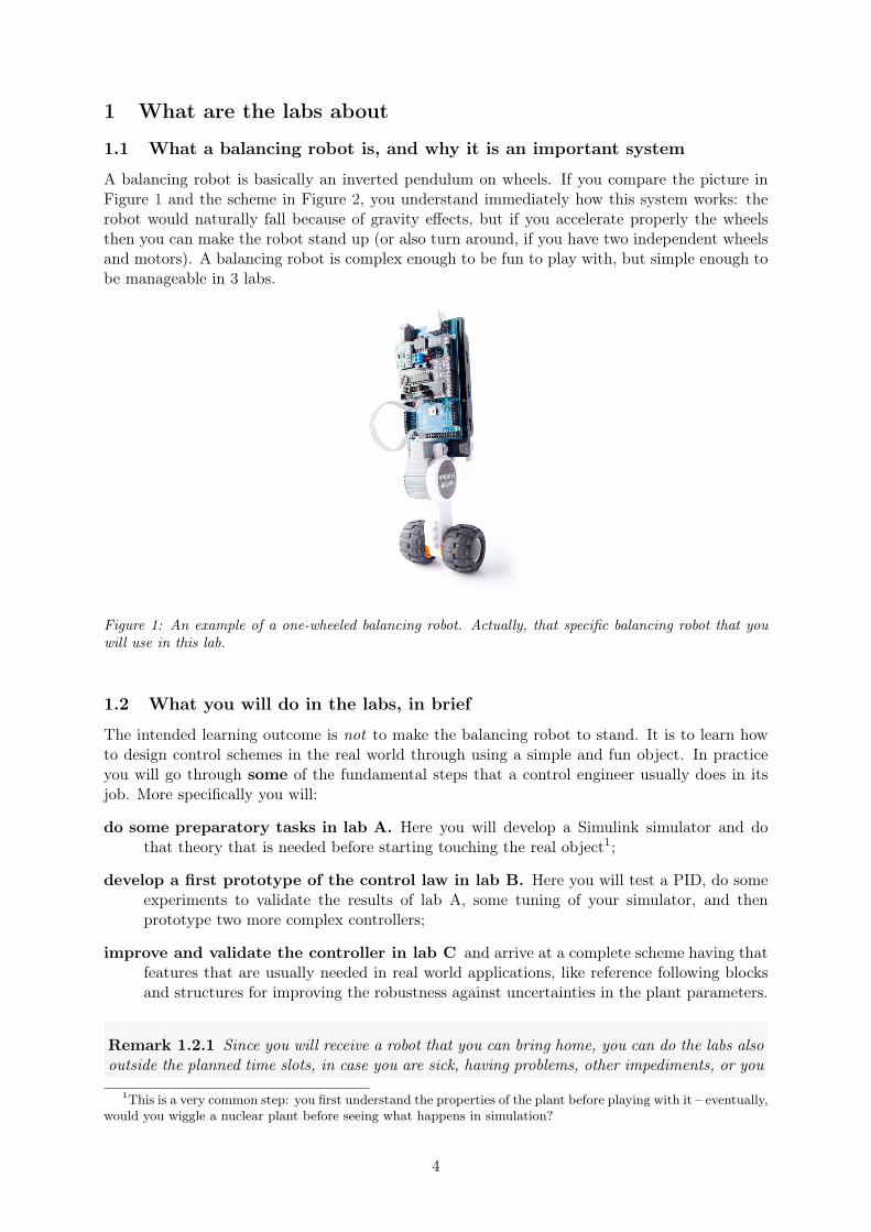
A balancing robot is basically an inverted pendulum on wheels. If you compare the picture inFigure 1 and the scheme in Figure 2, you understand immediately how this system works: therobot would naturally fall because of gravity effects, but if you accelerate properly the wheelsthen you can make the robot stand up (or also turn around, if you have two independent wheelsand motors). A balancing robot is complex enough to be fun to play with, but simple enough tobe manageable in 3 labs.

Figure 1: An example of a one-wheeled balancing robot. Actually, that specific balancing robot that youwill use in this lab.

1.2 What you will do in the labs, in brief

The intended learning outcome is not to make the balancing robot to stand. It is to learn howto design control schemes in the real world through using a simple and fun object. In practiceyou will go through some of the fundamental steps that a control engineer usually does in itsjob. More specifically you will:

do some preparatory tasks in lab A. Here you will develop a Simulink simulator and dothat theory that is needed before starting touching the real object1;

develop a first prototype of the control law in lab B. Here you will test a PID, do someexperiments to validate the results of lab A, some tuning of your simulator, and thenprototype two more complex controllers;

improve and validate the controller in lab C and arrive at a complete scheme having thatfeatures that are usually needed in real world applications, like reference following blocksand structures for improving the robustness against uncertainties in the plant parameters.

Remark 1.2.1 Since you will receive a robot that you can bring home, you can do the labs alsooutside the planned time slots, in case you are sick, having problems, other impediments, or you

1This is a very common step: you first understand the properties of the plant before playing with it – eventually,would you wiggle a nuclear plant before seeing what happens in simulation?

4

xw

ywθw

xb

yb

θb

lw = radius of the wheel

lb = body-wheel’s center distance

mw = mass of the wheel

mb = mass of the body

Figure 2: A simple schematic representation of a one-wheeled balancing robot where all the mass of robot(but the wheels’) is concentrated in its center of mass. The notation used in this figure is the notationused throughout the whole document.

want to do the labs before the others. We nonetheless suggest to attend the scheduled labs, sincethere you will have:

• the possibility of chatting with your peers and with the instructors;

• the guarantee of having people helping you with non-working hardware.

1.3 What you will do at home, in brief

You are supposed to work a bit also at home. More specifically:

1. read carefully this manual. If you have questions / doubts, ask before doing the labs(via email, via Skype, via coming to the offices of the instructors – you have the list of allthe possibilities in Section 9.9);

2. study the theory behind the assigned tasks. Below you will find some “tasks”, and each ofthem will indicate what you should know. Thus before coming to the labs please do:

(a) read the chapter relative to that lab;

(b) go through all the various tasks;

(c) study what they tell you to study.

1.4 How you will be evaluated, in brief

In brief, to pass R7003E one needs to pass also the labs. More precisely, to pass the labsone needs to hand in:

5

1. the reports of the 3 labs;

2. the final report;

3. the material associated to the demo,

and get sufficient grades in the reports plus have a working demo. In details, read Section 8 andyou will find all the necessary information. For now you should know that it is mandatory tohand in the reports and the demo material to have the course registered. Notice that you donot need to hand in the material before doing the exam, and that there are no expiration dates:you can do the exam in 2016 and hand in the material in 2215, or vice-versa2. Of course in thatcase you get the exam registered in 2215.

Notice also that normally the labs will not contribute to the overall final grading of the wholeexam, and will act as a go / no go flag: you pass the exam when you pass also the labs, butgetting “sufficient” or “excellent” grades in the labs will not change the overall grading.

An important exception is the one described in Section 8.3, for which who hands in thereports and the demo in time (and get at least a “sufficient” everywhere) gets some additionalpoints with a rule that is, more or less, “the better grades you get in the reports, the moreadditional points you get in the overall grading” (see Equation (31) on page 62 for a quickreference).

More information in Section 8.

1.5 How we would like you to interact with your peers

Each group should be composed of maximum 3 persons each.

Thus if you want to be in 2 it is ok (you will work harder but you will also learn better3). Wediscourage you to be in 1 (but you are allowed to do so, if you want / need to). We delegatethe process of creating the groups to you – in other words, try to self-organize. If somebody hassome difficulty in finding a group let us know.

Please, help each other not only internally in the group but also among groups: discuss ideasand approaches, exchange information, compare results. Specially, brainstorm together and trynew things – there exist almost4 no stupid approach. Notice that you may also form inter-groupscollaborations for solving some optional tasks (more information in Section 7).

PS: do not cheat; first, we understand it. Second, let’s be grown ups.

1.6 How we would like you to interact with us

Golden rules:

• feel free to ask for both help and clarifications (see Section 9.9 for our contacts);

• tell us (as soon as possible) if something in this manual is not clear / contradictory /incomplete;

• tell us (as soon as possible) if something does not work (balancing robot, computers, etc.);

• tell us (whenever you prefer) your opinions and suggestions (we care about this much morethan one would expect).

To summarize these rules with a chart:

2If the course will still be there – if not you lose everything.3No additional points for this, sorry.4Almost. A classical counterexample is putting the device on fire, something that has been proved not helping

controlling it.

6

we believe in feedback

7

2 How to read this manual

The document is structured as follows:

• Sections 1 and 2 overview some general information;

• Sections 3, 4 and 5 list the tasks that you are supposed to do;

• Section 6 describes the demo you will do after the labs;

• Section 7 lists some optional tasks that you may want to do if you feel like (more info inthat section);

• Section 8 describes how to report your findings;

• Section 9 presents some ancillary information and links.

2.1 How to complete the assigned tasks

The labs are divided in subsections. Each subsection in its turn contains tasks instructions,reading assignments and reporting instructions like the following ones:

Task 2.1.1 do this, do that.

Reading 2.1 read this, study that.

Reporting 2.1.1 plot this, comment that.

The tasks indicate what you are supposed to do in the lab, the readings suggest what youshould know of the textbook to perform the tasks, while the reportings summarize what toreport and how. Often you will be asked to report something in either parametric or numericforms (or both). This means the following:

parametric form: you express the quantity as a function of some parameters, e.g.,

A =

aij

, aij = mbglb + Ib (1)

numeric form: you express the quantity with its numerical value, e.g.,

A =

3.25

(2)

Table 4 summarizes the values of the parameters describing your balancing robot.Notice that every task, reading or report is identified by an ID so that when we communicate

among us we can be always on the same page of the same book. Once again, if some task, readingor reporting is unclear, contact us as soon as possible (Section 9.9). More information on howto report your findings is also in Section 8.

8

Remark 2.1.1 Our advice is to do not try to complete the reporting during the labs.Instead simply solve the tasks, and every time that you use Matlab or Simulink savethe workspace after you completed a task, giving to the saved workspace a name likeworkspace_task_4.1_year_month_day_hour.mat. In this way you will save all the informa-tion available that is needed to do the reporting comfortably at home (moreover you will notoverwrite potentially important data). And do backups of everything every time (or usedropbox or dropbox-like services, an excellent alternative to manual backups).

2.2 Notation

You are imposed to use the notation in Table 5 (page 69). Not following the notation =⇒failing the labs.

9

3 Lab A

The main purpose of this lab is to develop a simulator of the balancing robot that will thenbe used in the next labs for rapid debugging an prototyping purposes. Instrumental to thedevelopment of the simulator you are supposed to start with describing mathematically thesystem. The reporting for this section should be done following the corresponding template (seeSection 8). Notice that this lab does not require you to be physically at the University, and youcan do it whenever / wherever you want (as soon as you have Matlab and Simulink installed).

3.1 Derive the Equations of Motion

Our first step towards having a simulator of the balancing robot is to derive the Equations ofMotion (EOM) of the system. To this aim you should read:

Reading 3.1

• Section 2.1

• Section 2.3.2

• Section 3.1.7

• Section 3.3

of the textbook.We model the balancing robot as in Figure 3 (check also the table for the notation on page 69):

the body of the robot is a thin pole with its mass mb concentrated only in the center of mass ofthe robot, and with this mass being distant lb from the center of the wheel. In its turn the wheelhas radius lw, and mass mr.

The aim of this subsection is then to find the dynamics for the position of the wheel xw andthe angle of the body θb given the voltage vm in input to the motor. Mathematically, we needto express the system as xw = fxw

(xw, xw, θb, θb, θb, vm

)θb = fθb

(xw, xw, xw, θb, θb, vm

) (3)

for opportune functions fxw and fθb (notice that we need two equations since we have twovariables). To this aim we make the following assumptions:

1. the robot moves in a flat and horizontal environment, i.e., yw = 0 always;

2. the wheels never slip and the robot is never turned around by external factors, i.e., xw =lwθw always;

3. the aerodynamic frictions are negligible;

4. the unique force that can be commanded by us is the torque applied by the motor to thewheel, and this torque is driven by the voltage that is applied to the motor.

Remark 3.1.1 There are a lot of different equivalent ways of finding EOMs of mechanicalsystems. In the following we suggest you to use Newton laws, but you are absolutely free toderive however you want. In case you do not feel like following the suggestions below, as analternative task you have to describe how you derived instead.

10

xw

ywθw

xb

yb

θb

lw = radius of the wheel

lb = body-wheel’s center distance

mw = mass of the wheel

mb = mass of the body

Figure 3: A simple schematic representation of a one-wheeled balancing robot where all the mass of robot(but the wheels’) is concentrated in its center of mass (repetition of Figure 2 on page 5, for readabilityconvenience).

If we use a Newton laws based approach to the modeling of the EOM, we can follow these 3steps:

1. derive the dynamics of the wheel, i.e., how a torque applied to the wheel transforms intotranslation and forces applied to the body;

2. derive the dynamics of the body, i.e., how a force applied to the body transforms intodynamics of its center of mass;

3. derive the dynamics of the motor, i.e., how the voltage applied to the motor transformsinto a torque applied to the wheel.

It is simple to find (3) by following this workflow: a) derive the dynamics of the wheel and ofthe body independently keeping the motor’s torque Tm inside the equations; b) combine the twodynamics into an unique dynamics with the structure (3) but with Tm instead of the voltage vm(that is actually our input); c) derive the dynamics of the torque Tm as a function of vm; d) plugin the solution of c) in the solutions of b) and obtain a dynamics with the structure (3).

Remark 3.1.2 Be careful at the quantities that are considered in the various tasks: pay spe-cially attention at the subscripts, and remember that w means “wheel”, b means “body”, m means“motor”.

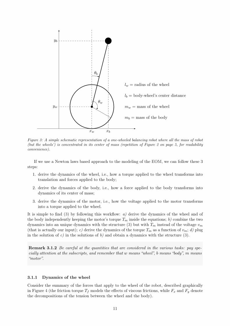
3.1.1 Dynamics of the wheel

Consider the summary of the forces that apply to the wheel of the robot, described graphicallyin Figure 4 (the friction torque Tf models the effects of viscous frictions, while Fx and Fy denotethe decompositions of the tension between the wheel and the body).

11

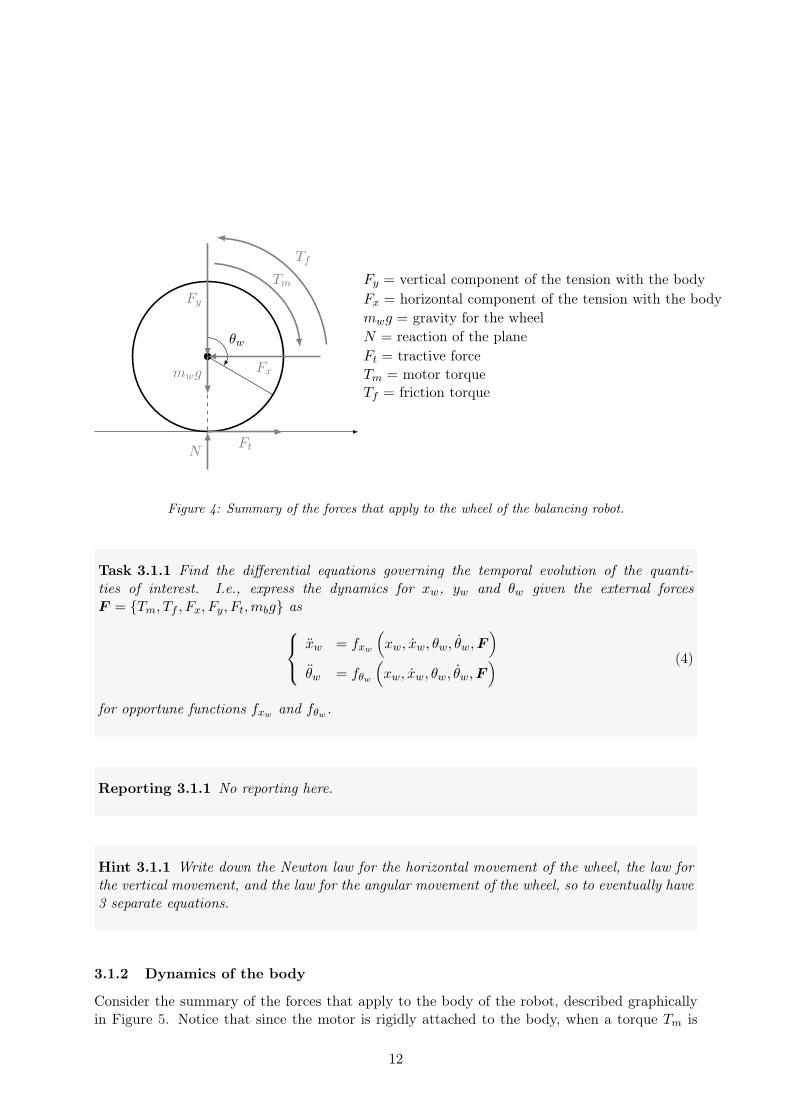
θw

mwg

NFt

Fx

Fy

Tm

Tf

Fy = vertical component of the tension with the bodyFx = horizontal component of the tension with the bodymwg = gravity for the wheelN = reaction of the planeFt = tractive forceTm = motor torqueTf = friction torque

Figure 4: Summary of the forces that apply to the wheel of the balancing robot.

Task 3.1.1 Find the differential equations governing the temporal evolution of the quanti-ties of interest. I.e., express the dynamics for xw, yw and θw given the external forcesF = {Tm, Tf , Fx, Fy, Ft,mbg} as xw = fxw

(xw, xw, θw, θw,F

)θw = fθw

(xw, xw, θw, θw,F

) (4)

for opportune functions fxw and fθw .

Reporting 3.1.1 No reporting here.

Hint 3.1.1 Write down the Newton law for the horizontal movement of the wheel, the law forthe vertical movement, and the law for the angular movement of the wheel, so to eventually have3 separate equations.

3.1.2 Dynamics of the body

Consider the summary of the forces that apply to the body of the robot, described graphicallyin Figure 5. Notice that since the motor is rigidly attached to the body, when a torque Tm is

12

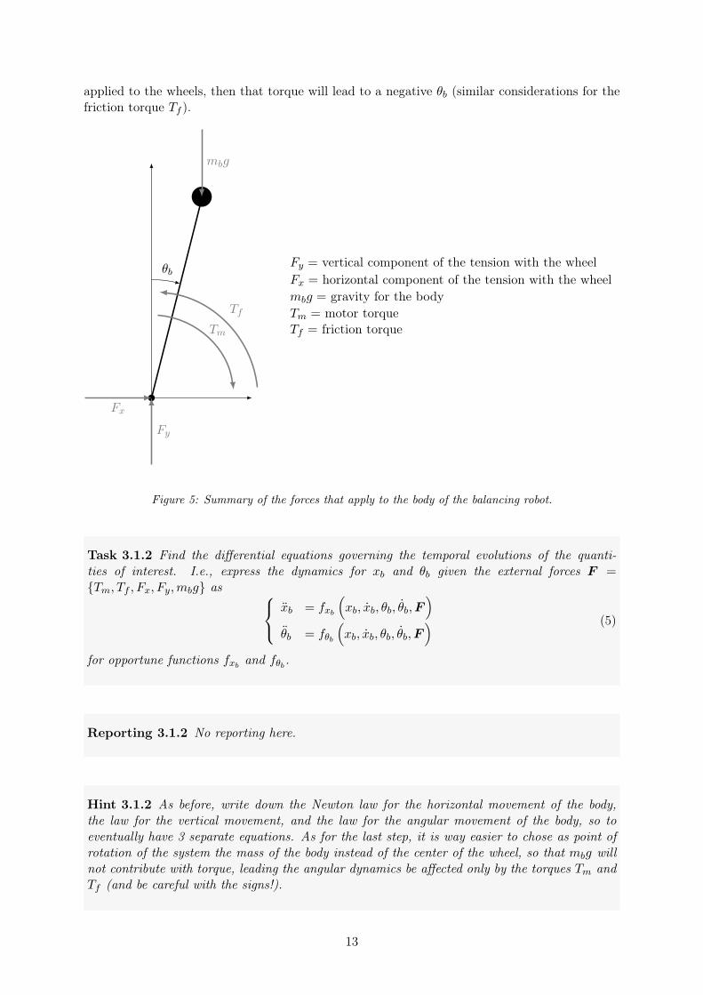
applied to the wheels, then that torque will lead to a negative θb (similar considerations for thefriction torque Tf ).

θb

Fy

Fx

mbg

Tm

Tf

Fy = vertical component of the tension with the wheelFx = horizontal component of the tension with the wheelmbg = gravity for the bodyTm = motor torqueTf = friction torque

Figure 5: Summary of the forces that apply to the body of the balancing robot.

Task 3.1.2 Find the differential equations governing the temporal evolutions of the quanti-ties of interest. I.e., express the dynamics for xb and θb given the external forces F ={Tm, Tf , Fx, Fy,mbg} as xb = fxb

(xb, xb, θb, θb,F

)θb = fθb

(xb, xb, θb, θb,F

) (5)

for opportune functions fxband fθb.

Reporting 3.1.2 No reporting here.

Hint 3.1.2 As before, write down the Newton law for the horizontal movement of the body,the law for the vertical movement, and the law for the angular movement of the body, so toeventually have 3 separate equations. As for the last step, it is way easier to chose as point ofrotation of the system the mass of the body instead of the center of the wheel, so that mbg willnot contribute with torque, leading the angular dynamics be affected only by the torques Tm andTf (and be careful with the signs!).

13

Given the two systems (4) and (5) we now seek to get closer to (3) by finding a systemwhere the unique variables considered are xw and θb, and where the internal tension forces Fx

and Fy and the tractive force Ft disappear from the dynamics. In other words, we now seek tocombine (4) and (5) so to derive something like xw = fxw

(xw, xw, θb, θb, θb, Tm, Tf

)θb = fθb

(xw, xw, xw, θb, θb, Tm, Tf

) (6)

for opportune functions fxw and fθb (notice: since we are considering two variables we need twoequations). In other words, we need to eliminate all the variables that are not xw and θb.

Task 3.1.3 Combine and rewrite (4) and (5) into a system like (6).

Reporting 3.1.3 No reporting here.

Hint 3.1.3 The task is essentially to take all the variables that are not xw and θb in theequations that have been obtained before and write them as functions of xw, θb, Tm and Tf .

To this aim we can use two separate facts: first,

θw = xw/lw, (7)

and this will be very useful in the Newton law for the angular movement of the wheel.Second, to rewrite Ft, Fx and Fy we can directly use the Newton laws for the linear move-

ments of the wheel and of the body. If everything goes as expected then there will be the needfor simplifying the quantity “ yb sin (θb)− xb cos (θb)”. To this aim one can exploit the followingequivalences:

xb = xw + lb sin (θb)

xb = xw + θblb cos (θb)

xb = xw + θblb cos (θb)− θ2b lb sin (θb)yb = yw + lb cos (θb)

yb = yw − θblb sin (θb) = −θblb sin (θb)

yb = −θblb sin (θb)− θ2b lb cos (θb)

(8)

Before continuing we then consider that Tf is a torque due to mechanical frictions, and thatthus is proportional to the rotational speed of the motor, i.e.,

Tf = bf

(θw − θb

)= bf

(xwlw

− θb

). (9)

We can thus make immediately this substitution in the solution of Task 3.1.3 and arrive at aform of the type xw = fxw

(xw, xw, θb, θb, θb, Tm

)θb = fθb

(xw, xw, xw, θb, θb, Tm

) (10)

instead of the type (6).

14

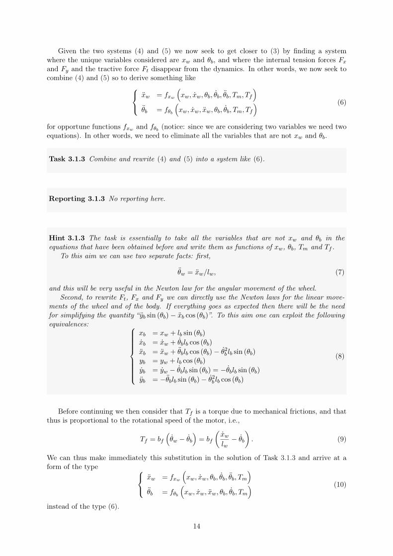
3.1.3 Dynamics of the motor

The final step is to express the torque Tm as a function of vm, so that we can modify (6) to arriveto our final (3). Consider then that our motor is a Direct Current (DC) motor schematizable asin Figure 6.

vm

RmimLm

Keθm

Tm

Figure 6: Schematic representation of a DC motor. Here θm indicates the angle of the motor (that, inour case, will be a function of θw and θb. . . )

Task 3.1.4 Find the differential equations governing the temporal evolution of the quantitiesof interest assuming the inductance Lm and the motor viscous coefficient bm negligible. I.e.,express the relation of Tm with vm, xw and θb as

Tm = fTm

(vm, xw, θb

)(11)

for an opportune function fTm .

Reporting 3.1.4 No reporting here.

Hint 3.1.4 Do as the textbook does.

Now we have all the ingredients to derive (3) in a symbolic form. Notice that it is not yettime to substitute the symbols with the values provided in Table 4.

Task 3.1.5 Plug (9) and (11) into (6) and obtain (3) in a symbolic form.

Reporting 3.1.5 Report the final EOMs you computed.

15

3.2 Linearize the Equations of Motion

If you did everything right, you should get the following non-linear terms:

• sin (θb);

• xw cos (θb);

• θb cos (θb);

• θ2b sin (θb).

Since up to know you know how to build controllers only for linear systems5, we need to linearizeour EOM. To do so you may need to refresh how to linearize a system:

Reading 3.2

• Section 9.2.1;

• lecture notes of lesson TODO.

Now you are ready to solve the following:

Task 3.2.1 Linearize the EOM around an opportunely chosen point, assuming that centripetalforces are negligible.

Reporting 3.2.1 1. say which linearization point you choose;

2. say why you choose that specific point;

3. write the linearized EOM.

5If you want to know more about control of non-linear systems then consider attending also the course R70xxEin 2017 LP1.

16

3.3 Write the linearized Equations of Motion in State-Space form

Reading 3.3

• Section 7.2.

Since this course is focused on control based on State-Space (SS) models, we do now rewrite ourEOM as {

x = Ax+Buy = Cx+Du

(12)

for opportune x, A, B, C and D. As for the input and output, assume for now:

u = vmy = θb

(13)

In other words, for now our input is the voltage applied to the motor, while for now the measureis the angular deviation of the balancing robot from the vertical upright position.

Task 3.3.1 Write the linearized EOM as in (12) considering the inputs and outputs as in (13).

Reporting 3.3.1 1. say what is your choice for x;

2. write the matrices A, B, C and D in (12) in parametric form;

3. write the matrices A, B, C and D in (12) in parametric numeric form (for this purposeuse Table 4 on page 68).

Hint 3.3.1 It is much easier and numerically stable6 to do as follows:

1. write the system in parametric form as

[γ11 γ12γ21 γ22

] [xwθb

]=

[α11 α12 α13 α14

α21 α22 α23 α24

]xwxwθbθb

+

[β1β2

]u (14)

where the various γ, α and β are functions of the various parameters in Table 4 (e.g.,and this is just an example, α23 = Ib +mr +Rm);

2. write in Matlab a script where you first copy the code

g = 9.8;b_f = 0;m_b = 0.381;l_b = 0.112;I_b = 0.00616;

17

m_w = 0.036;l_w = 0.021;I_w = 0.00000746;R_m = 4.4;L_m = 0;b_m = 0;K_e = 0.444;K_t = 0.470;

and then you write down all the various αij = . . .. In this way you will compute your γs,αs and βs immediately;

3. since

[xwθb

]=

[γ11 γ12γ21 γ22

]−1 [α11 α12 α13 α14

α21 α22 α23 α24

]xwxwθbθb

+

[γ11 γ12γ21 γ22

]−1 [β1β2

]u (15)

you can create your A, B, C variables in Matlab immediately with a minimum of manip-ulation of the equations above (do all these computations in Matlab! And try to learn howto use symbolic variables).

18

3.4 Determine the transfer function relative to system (12)

Here you need again:

Reading 3.4

• Section 7.4.

Task 3.4.1 Compute the transfer function, the poles and the zeros of the system.

Before using Matlab, we suggest you to start by getting an intuition of which poles and thezeros you will get by analyzing the structure of

sI −A and[sI −A −B

C D

]. (16)

Only after this use Matlab (and the commands in Table 3 on page 66) to compute the requestedquantities both analytically and numerically. The rationale for this prior checking is this one:Matlab (actually, any software) has numerical problems induced by the fact that they use finitearithmetic7, and may thus make mistakes. You can then notice and correct them only if youdeveloped intuitions of what you should get and what you should not.

Reporting 3.4.1 1. write the transfer function in the form

G(s) = K

∏i (s− zi)∏j (s− pj)

(17)

2. describe, in case you saw them, whether you experienced some numerical problem withMatlab.

Once again we suggest you to use Matlab and the workspace loaded before.

7Read, e.g., the paragraph “Zeros at Infinity” in http://ctms.engin.umich.edu/CTMS/index.php?aux=Extras_Conversions.

19

3.5 Design a PID controller stabilizing the transfer function computed inSection 3.4

Reading 3.5

• Section 4.3.

It is important to notice the following things:

1. at this stage we just want to stabilize the transfer function from the motor voltage vm tothe body angle θb; in other words, we are designing a PID that makes the robot do notfall. Thus our reference signal for θb is zero;

2. nothing is said about xw. For now we are ignoring what happens to the position (in the xaxis) of the robot;

3. plotting the root locus of the linearized balancing robot indicates that there is no P con-troller stabilizing θb starting from vm. A PI can, but the stability domain is going to bevery small. A PID instead works much better and gives a much bigger stability domain.We thus use a PID as our first initial choice.

Task 3.5.1 Design the PID using the poles allocation method. Since we are doing simulations,you are free to choose to set the poles wherever you want (as soon as the closed loop is stable,of course).

Reporting 3.5.1 1. Describe your choice for the poles, and what you want to achieve interms of impulse response for the closed loop system;

2. write the values of the parameters of the PID;

3. write the resulting closed loop function in its numerical form;

4. plot the impulse response and the Bode plot of the closed loop system.

If you have the possibility, compare your impulse response and Bode plots with the ones ofyour peers, discuss your choices, and think together at what will happen when you will implementyour controller on the real robot.

Importantly, after stabilizing the plant one should compute the stability margins for thelinear approximation of the closed loop system. These margins provide an indication of whetherthe balancing robot is expected to fall even under mild external disturbances.

Task 3.5.2 Compute the phase and gain margins for the linear approximation of the closedloop system.

20

Reporting 3.5.2 1. Draw the Nyquist diagram for the linearized balancing robot in feedbackwith the designed PID controller;

2. write the values of the phase and stability margins.

21

3.6 Model the effect of disturbing the robot

Reading 3.6 No readings here!

When controlling a system it may be meaningful to analyze the effects of that disturbances thatwill affect the normal operations of the plant. In our case we may want to check what happensif somebody pokes the robot, i.e., applies an impulsive horizontal force to the center of mass ofthe body of the balancing robot. In practice, we would like to know what happens if there is aterm in Figure 5 that sums with Fx.

Task 3.6.1 Modify the EOM of your balancing robot so to include an other additional inputthat is called d and that models somebody poking the robot. Derive also the linearized and statespace versions of these EOM.

Reporting 3.6.1 1. write the novel EOM in parametric form;

2. write the novel linearized EOM in state space in numerical form.

Hint 3.6.1 The poke affects the body, thus it affects the Newton laws of the dynamics of thebody. Moreover, the poke is “horizontal”. . .

You should now notice that the novel disturbance can be thought as an additional input,but that this new input d is different from the voltage vm. Indeed in the new state spacerepresentation the two columns of B are not linearly dependent, and this means that d and vm“enter” the state of the system with a “different angle” (think geometrically). In practice, pokingthe robot is different from disturbing the voltage vm.

22

3.7 Check if everything is working as it should be

Reading 3.7 No readings here!

We have now all the ingredients to start checking if things are working as expected. The tasknow is to simulate what the linear systems does when it is subject to a small poke.

Task 3.7.1 Implement a Simulink simulator for the linearized balancing robot subject to thetwo inputs vm and d. Consider as outputs of the system all the states of the balancing robot,i.e., use as matrices C and D the matrices

C =

1 0 0 00 1 0 00 0 1 00 0 0 1

D =

0 00 00 00 0

. (18)

Perform an experiment for which the external disturbance d is

d(t) =

{0.1 for t ∈ [0, 0.1]0 otherwise, (19)

and check the values of the signals θb and xw.

To create d(t) you may use the Simulink block Signal Builder. For the linearized robots dy-namics we instead suggest to use a LTI System that loads its A, B, C and D matrices from Matlab’sworkspace. Be careful that here B includes not only the input vm but also the input (disturbance)d, so update your definitions of C and D accordingly (as above). We suggest to implement thePID through a PID Controller block; this block requires to set the Filter coefficient (N),and if you do not know what it does then check Simulink’s help and try to think at what happensif N is very big or very small.

Important: we strongly discourage you to hard-code Simulink’s blocks8. Moreover wesuggest also to automate the production of figures, e.g., as we did in Section 9.3 on page 63.

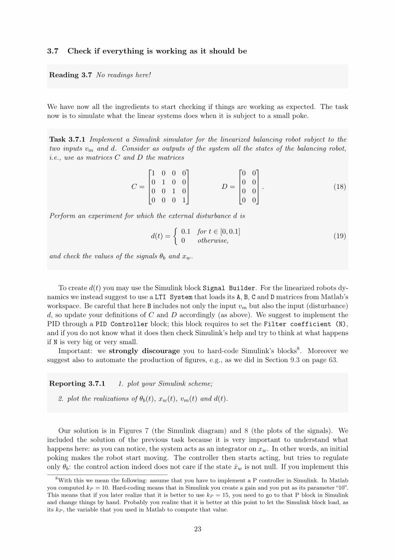
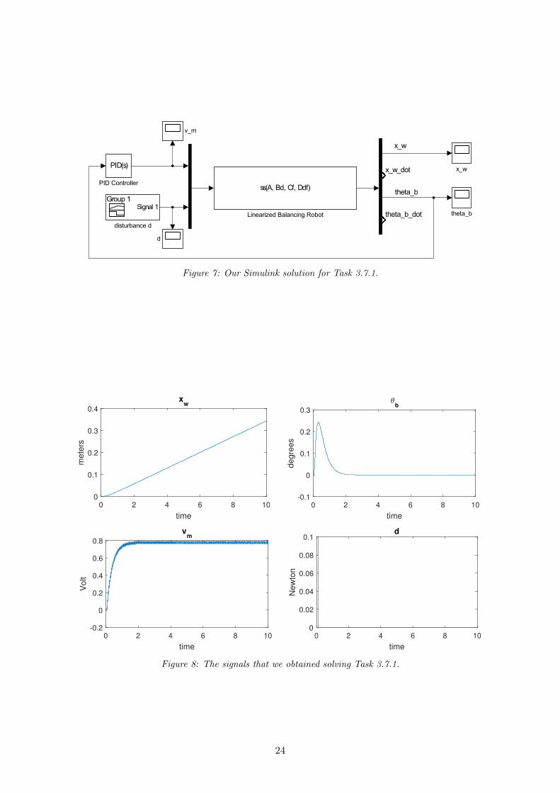
Reporting 3.7.1 1. plot your Simulink scheme;

2. plot the realizations of θb(t), xw(t), vm(t) and d(t).

Our solution is in Figures 7 (the Simulink diagram) and 8 (the plots of the signals). Weincluded the solution of the previous task because it is very important to understand whathappens here: as you can notice, the system acts as an integrator on xw. In other words, an initialpoking makes the robot start moving. The controller then starts acting, but tries to regulateonly θb: the control action indeed does not care if the state xw is not null. If you implement this

8With this we mean the following: assume that you have to implement a P controller in Simulink. In Matlabyou computed kP = 10. Hard-coding means that in Simulink you create a gain and you put as its parameter “10”.This means that if you later realize that it is better to use kP = 15, you need to go to that P block in Simulinkand change things by hand. Probably you realize that it is better at this point to let the Simulink block load, asits kP , the variable that you used in Matlab to compute that value.

23

theta_b_dot

theta_b

x_w

x_w_dot

ss(A, Bd, Cf, Ddf)

Linearized Balancing Robot

PID(s)

PID Controller

x_w

theta_bSignal 1

Group 1

disturbance d

d

v_m

Figure 7: Our Simulink solution for Task 3.7.1.

time

0 2 4 6 8 10

me

ters

0

0.1

0.2

0.3

0.4

xw

time

0 2 4 6 8 10

de

gre

es

-0.1

0

0.1

0.2

0.3

θb

time

0 2 4 6 8 10

Vo

lt

-0.2

0

0.2

0.4

0.6

0.8

vm

time

0 2 4 6 8 10

Ne

wto

n

0

0.02

0.04

0.06

0.08

0.1d

Figure 8: The signals that we obtained solving Task 3.7.1.

24

PID in your robot thus you should expect to run after it all the time. In mathematical terms,the system is actually still unstable.

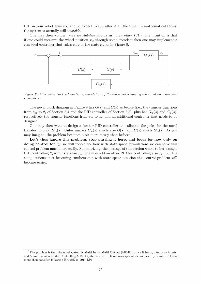
One may then wonder: may we stabilize also xb using an other PID? The intuition is thatif one could measure the wheel position xw through some encoders then one may implement acascaded controller that takes care of the state xw as in Figure 9.

r Gw(s)

G(s)C(s)

Cw(s)

+−

+ vm xw−

Figure 9: Alternative block schematic representation of the linearized balancing robot and the associatedcontrollers.

The novel block diagram in Figure 9 has G(s) and C(s) as before (i.e., the transfer functionsfrom vm to θb of Section 3.4 and the PID controller of Section 3.5), plus has Gw(s) and Cw(s),respectively the transfer functions from vm to xw and an additional controller that needs to bedesigned.

One may then want to design a further PID controller and allocate the poles for the noveltransfer function Gw(s). Unfortunately Cw(s) affects also G(s), and C(s) affects Gw(s). As youmay imagine, the problem becomes a bit more messy than before9.

Let’s thus ignore this problem, stop pursing it here, and focus for now only ondoing control for θb: we will indeed see how with state space formulations we can solve thiscontrol problem much more easily. Summarizing, the message of this section wants to be: a singlePID controlling θb won’t stabilize xw; one may add an other PID for controlling also xw, but thecomputations start becoming cumbersome; with state space notation this control problem willbecome easier.

9The problem is that the novel system is Multi Input Multi Output (MIMO), since it has vm and d as inputs,and θb and xm as outputs. Controlling MIMO systems with PIDs requires special techniques; if you want to knowmore then consider following R70xxE in 2017 LP1.

25

3.8 Convert the controller to the discrete domain

Let’s then focus to the problem of implementing C(s) in our real balancing robot. Beforeproceeding, we notice that the Arduino board is a digital controller – in other words, you cannotimplement C(s) as it is; you must discretize it. How? Let’s start by reading the following:

Reading 3.8

1. Pages 335-336;

2. Section 8.3.2;

3. Section 8.3.6.

As you know from there are several discretization methods. For now we focus on Zero OrderHold (ZOH) methods, and defer more considerations for Lab C.

Task 3.8.1 Compute the bandwidth of the linearized balancing robot, and decide the samplingperiod of the digital controller. Compute then the controller in terms of difference equations.

Reporting 3.8.1 1. report the bandwidth of the system;

2. report the chosen sampling time;

3. motivate your choice;

4. report the transfer function C(z) of your controller in its parametric form.

26

3.9 Simulate the closed loop system

Reading 3.9 No readings here!

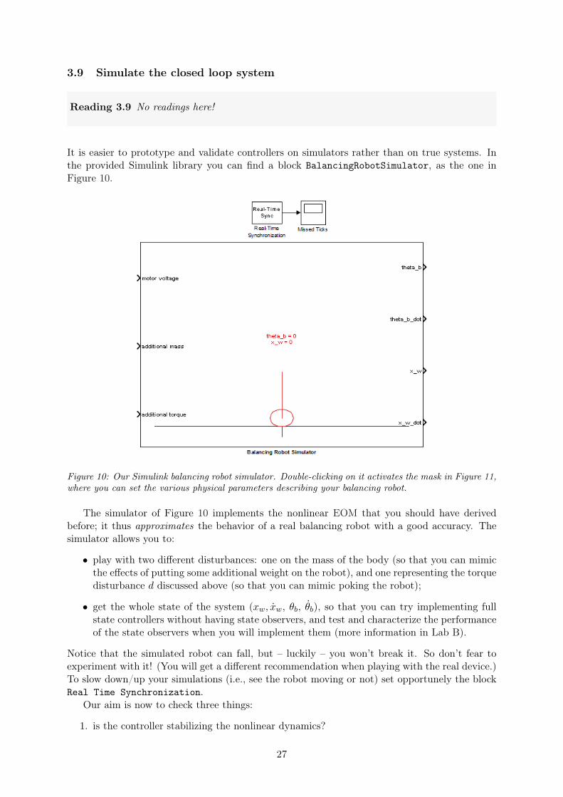
It is easier to prototype and validate controllers on simulators rather than on true systems. Inthe provided Simulink library you can find a block BalancingRobotSimulator, as the one inFigure 10.

Figure 10: Our Simulink balancing robot simulator. Double-clicking on it activates the mask in Figure 11,where you can set the various physical parameters describing your balancing robot.

The simulator of Figure 10 implements the nonlinear EOM that you should have derivedbefore; it thus approximates the behavior of a real balancing robot with a good accuracy. Thesimulator allows you to:

• play with two different disturbances: one on the mass of the body (so that you can mimicthe effects of putting some additional weight on the robot), and one representing the torquedisturbance d discussed above (so that you can mimic poking the robot);

• get the whole state of the system (xw, xw, θb, θb), so that you can try implementing fullstate controllers without having state observers, and test and characterize the performanceof the state observers when you will implement them (more information in Lab B).

Notice that the simulated robot can fall, but – luckily – you won’t break it. So don’t fear toexperiment with it! (You will get a different recommendation when playing with the real device.)To slow down/up your simulations (i.e., see the robot moving or not) set opportunely the blockReal Time Synchronization.

Our aim is now to check three things:

1. is the controller stabilizing the nonlinear dynamics?

27

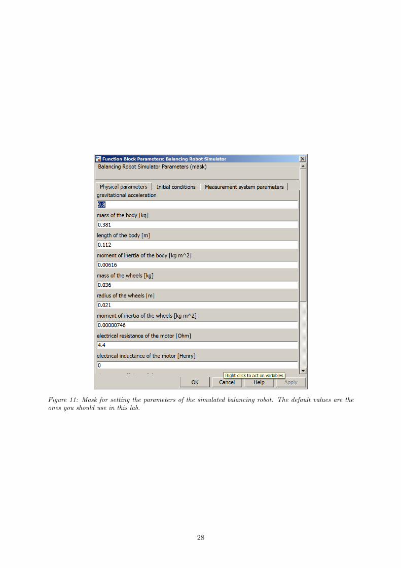
Figure 11: Mask for setting the parameters of the simulated balancing robot. The default values are theones you should use in this lab.

28

2. is the linearized dynamics a good approximation of the nonlinear ones?

3. is the chosen sampling time good for control purposes?

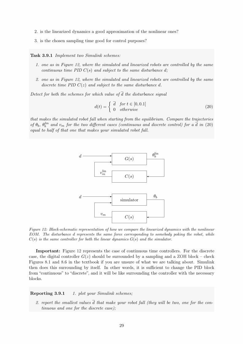
Task 3.9.1 Implement two Simulink schemes:

1. one as in Figure 12, where the simulated and linearized robots are controlled by the samecontinuous time PID C(s) and subject to the same disturbance d;

2. one as in Figure 12, where the simulated and linearized robots are controlled by the samediscrete time PID C(z) and subject to the same disturbance d.

Detect for both the schemes for which value of d the disturbance signal

d(t) =

{d for t ∈ [0, 0.1]0 otherwise

(20)

that makes the simulated robot fall when starting from the equilibrium. Compare the trajectoriesof θb, θlin

b and vm for the two different cases (continuous and discrete control) for a d in (20)equal to half of that one that makes your simulated robot fall.

simulator

C(s)

G(s)

C(s)

d

d

vm

θb

vlinm

θlinb

Figure 12: Block-schematic representation of how we compare the linearized dynamics with the nonlinearEOM. The disturbance d represents the same force corresponding to somebody poking the robot, whileC(s) is the same controller for both the linear dynamics G(s) and the simulator.

Important: Figure 12 represents the case of continuous time controllers. For the discretecase, the digital controller G(z) should be surrounded by a sampling and a ZOH block – checkFigures 8.1 and 8.6 in the textbook if you are unsure of what we are talking about. Simulinkthen does this surrounding by itself. In other words, it is sufficient to change the PID blockfrom “continuous” to “discrete”, and it will be like surrounding the controller with the necessaryblocks.

Reporting 3.9.1 1. plot your Simulink schemes;

2. report the smallest values d that make your robot fall (they will be two, one for the con-tinuous and one for the discrete case);

29

3. plot θb(t), vm(t), θlinb (t) and vlin

m (t) (again, one for the continuous and one for the discretecase);

4. discuss what you understood from these experiments, and if (and how) it helped you tuningthe PID controller.

Troubleshooting:

• managing the sampling times in Simulink may be a hassle. Consider reading Section 9.6before moving from continuous time domains to discrete time domains;

• moving from continuous to discrete may also introduce numerical problems, e.g., make astable plant “explode”10. If this happens to you, then consider changing the “Discrete timesettings” of your PIDs (set, e.g., to “Backward Euler” or “Trapezoidal”. We will understandbetter what this means towards the end of the course).

Notice that the results you got in this last step may be indicating that your controller is notgood enough. Try playing with different gains (or, equivalently, with different positions of thepoles in the PID design step) and check how things change.

10It is because in our case we have a double integrator and numerical perturbations may be fatal for Simulink.

30

3.10 (Optional) play with the simulator

This is something you are not compelled to do, but that of course is (we think) a very usefulexercise. Our suggestion is to play around with the parameters in the simulator (i.e., make therobot heavier, put bigger wheels, lighter wheels, more powerful motors, etc.) and see if yourintuitions work. In other words, try to think “what is going to happen if I do this?” and doublecheck with experiments if you have understood how the system works. (And if you find somethingthat is worth to be mentioned in the lab report, of course mention it.)

31

4 Lab B

The main purpose of this lab is to start designing controllers using continuous time concepts. Inother words, you do not start immediately from discrete considerations but rather from contin-uous ones, and then discretize the results.

4.1 How to do tests on the robot

Reading 4.1 No readings here!

There are two different ways of running tests:

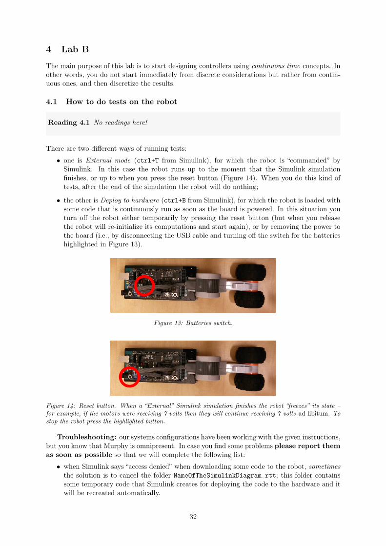
• one is External mode (ctrl+T from Simulink), for which the robot is “commanded” bySimulink. In this case the robot runs up to the moment that the Simulink simulationfinishes, or up to when you press the reset button (Figure 14). When you do this kind oftests, after the end of the simulation the robot will do nothing;

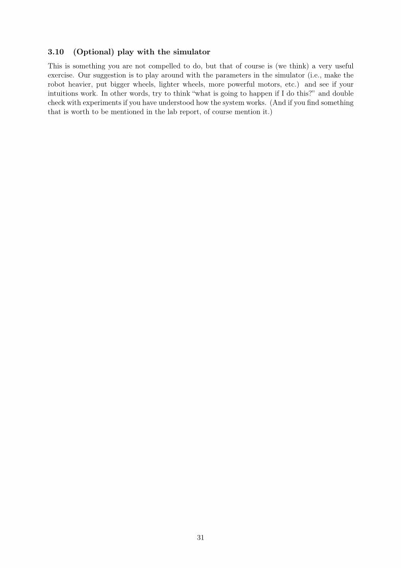
• the other is Deploy to hardware (ctrl+B from Simulink), for which the robot is loaded withsome code that is continuously run as soon as the board is powered. In this situation youturn off the robot either temporarily by pressing the reset button (but when you releasethe robot will re-initialize its computations and start again), or by removing the power tothe board (i.e., by disconnecting the USB cable and turning off the switch for the batterieshighlighted in Figure 13).

Figure 13: Batteries switch.

Figure 14: Reset button. When a “External” Simulink simulation finishes the robot “freezes” its state –for example, if the motors were receiving 7 volts then they will continue receiving 7 volts ad libitum. Tostop the robot press the highlighted button.

Troubleshooting: our systems configurations have been working with the given instructions,but you know that Murphy is omnipresent. In case you find some problems please report themas soon as possible so that we will complete the following list:

• when Simulink says “access denied” when downloading some code to the robot, sometimesthe solution is to cancel the folder NameOfTheSimulinkDiagram_rtt; this folder containssome temporary code that Simulink creates for deploying the code to the hardware and itwill be recreated automatically.

32

4.2 Communicating with the balancing robot

Reading 4.2 No readings here!

We start by checking if we are able to communicate with the robot. To this aim follow thesesteps:

1. download from http://staff.www.ltu.se/~damvar/R7003E-2016-LP2.html the code forlab B (it is a .zip file, unzip it wherever you prefer);

2. connect the robot and the computer with the USB cable (no need for plugging the batteriesat this moment now);

3. check to which COM port the robot is connected by pressing the Windows key and checking“Devices and Printers”;

4. open Matlab;

5. create a Matlab startup script H:\My Documents\MATLAB\startup.m and add in it the lineof code addpath('C:\MATLAB\RASPlib'); (if you want you can also add other code – thisscript is what is executed when Matlab starts up);

6. change the working directory to the folder containing the extracted files (notice: it shouldbe a local folder, i.e. H:something and not \\afs\ltu.se\students\something otherwiseyou will get an error);

7. open Simulink (type simulink in Matlab’s command line and then “enter”), and then openthe Simulink file LabB_CheckCommunications.slx;

8. open the “Model Configuration Parameters” dialog (Ctrl+E), select “Run on Target Hard-ware”, set the COM port number to what Windows tells you, and then click the text “loadparameters”;

9. launch a simulation in external mode (ctrl+T);

10. stop manually the simulation whenever you want (notice that after stopping Simulink youshould also reset the robot by pressing the reset button highlighted in Figure 14 on page 32);

11. now you can check if you got the data from the robot in two different ways11:

(a) double-clicking on the scopes in the Simulink diagram (you can actually see the dataon-line);

(b) plot the signals in Matlab using, e.g., the following code:

figure(1)plot( tAngleFromGyro.time, tAngleFromGyro.signals.values, '-b' );axis([0, max(tAngleFromGyro.time), 100, 190]);legend('raw signal');title('measurements from the gyroscope'); xlabel('time (sec)'); ylabel('degrees');set(gcf, 'Units', 'centimeters');set(gcf,'Position',[1 1 11 9]);set(gcf, 'PaperPositionMode', 'auto');print('-depsc2', '-r300', 'raw_angle_from_gyro.eps');

11In our opinion visualizing with Simulink is more useful for debugging purposes; visualizing with Matlab isinstead better for reporting ones, since you can automate saving and moving figures as you like. Of course youare free to do as you wish.

33

(notice that you should have 4 signals in the workspace: from the accelerometer, thegyro, the encoder and the motor, and all of them should contain some information).

If you get meaningful plots then you successfully communicated with the robot.

34

4.3 Checking that reality is far from ideality

Reading 4.3 No readings here!

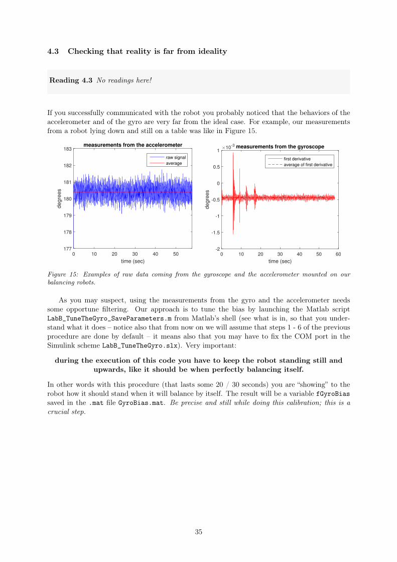
If you successfully communicated with the robot you probably noticed that the behaviors of theaccelerometer and of the gyro are very far from the ideal case. For example, our measurementsfrom a robot lying down and still on a table was like in Figure 15.

time (sec)

0 10 20 30 40 50

de

gre

es

177

178

179

180

181

182

183measurements from the accelerometer

raw signal

average

time (sec)

0 10 20 30 40 50 60

degre

es

×10-3

-2

-1.5

-1

-0.5

0

0.5

1measurements from the gyroscope

first derivative

average of first derivative

Figure 15: Examples of raw data coming from the gyroscope and the accelerometer mounted on ourbalancing robots.

As you may suspect, using the measurements from the gyro and the accelerometer needssome opportune filtering. Our approach is to tune the bias by launching the Matlab scriptLabB_TuneTheGyro_SaveParameters.m from Matlab’s shell (see what is in, so that you under-stand what it does – notice also that from now on we will assume that steps 1 - 6 of the previousprocedure are done by default – it means also that you may have to fix the COM port in theSimulink scheme LabB_TuneTheGyro.slx). Very important:

during the execution of this code you have to keep the robot standing still andupwards, like it should be when perfectly balancing itself.

In other words with this procedure (that lasts some 20 / 30 seconds) you are “showing” to therobot how it should stand when it will balance by itself. The result will be a variable fGyroBiassaved in the .mat file GyroBias.mat. Be precise and still while doing this calibration; this is acrucial step.

35

4.4 Test the PID controller

Reading 4.4 No readings here!

We now test if the developed PID controller behaves as one would wish in the real system. Todo so:

1. mount the batteries on the robot (you may want to use some tape to do not have them fallall the time);

2. turn on the batteries switch (i.e., towards “batt on”, see Figure 13);

3. connect the USB cable and check the number of your COM port;

4. open the Simulink diagram LabB_PIDOverRobot.slx, and fix the COM port issue in caseyou need;

5. open the various sub-diagrams and explore how we implemented the various things;

6. open the Matlab script LabB_PIDOverRobot_Parameters.m, and put in it your gains kP , kIand kD (you will find in it our default values). Do not touch the other variables;

7. launch LabB_PIDOverRobot_Parameters.m to load these parameters (you can do it directlyin Simulink by clicking on the load parameters text);

8. launch a “Deploy to hardware” simulation (Ctrl+B). If you completed the steps in Sec-tion 4.2 successfully you should have no problems here;

9. if the robot does not balance, try to change the PID coefficients as your intuition suggests;

10. to visualize or save data from the robot follow this procedure:

(a) open the Matlab script GetDataFromSerial.m;(b) edit the variable iCOMPort accordingly to your settings;(c) edit the variable fSamplingPeriod to the same value that you set in the Matlab script

LabB_PIDOverRobot_Parameters.m;(d) modify (if you want) the variables:

• iCommunicationTime, that dictates the duration of the experiment;• fPlotsUpdatesPeriod, that dictates how often the plots will be refreshed;

(e) launch GetDataFromSerial.m. Notice that this will cause the robot to re-start ;(f) at the end of the experiment you will get the information from the robot saved in the

workspace in the variable aafProcessedInformation (open PlotDataFromSerial.mand look at the code inside to understand what is what).

We expect your PID to do not perform too well (for example, ours was stand-ing maximum some 10 seconds). So do not lose too much time in wiggling with the PIDcontroller.

Task 4.4.1 Test your PID controller as above.

36

Reporting 4.4.1 Report an example of the xw, θb and u obtained with your best PID controller,and the parameters of the PID. Indicate also how long you got the robot stand before falling forthis controller.

Troubleshooting:

• when closing inopportunely the serial communications you may get problems in re-establishingthe connections again. E.g., you may get an error of the kind:

Opening the serial communications...Error using serial/fopen (line 72)Open failed: Port: COM7 is not available. Available ports: COM3, COM4, COM5, COM10.Use INSTRFIND to determine if other instrument objects are connectedto the requested device.

In this case you may solve the problem closing Matlab, unplugging the USB cable of therobot from the computer side, restarting Matlab and then reconnecting the robot.

37

4.5 Check the controllability and observability properties of the linearizedsystem (12)

To this aim it is better if you refresh your knowledge in:

Reading 4.5

• Section 7.4;

• Section 7.7.

Task 4.5.1 Compute and discuss the controllability and observability properties of the linearizedsystem (12) in numeric form.

Reporting 4.5.1 1. write the numerical values for C and O;

2. write the controllability and observability indexes;

3. if something is not controllable or observable:

(a) motivate why this happens;

(b) say how you would fix the problem;

(c) say how this affects the transfer function of the system.

38

4.6 Design a SS controller selecting the poles using a second order approxi-mation

We now start the process of designing the first continuous time state-space oriented controller.The steps will be the following:

1. pretending that we have information on all the state, construct two controllers:

• one by doing poles allocation;

• an other one by using a Linear-Quadratic Regulator (LQR) approach;

2. since we do not measure the full state of the system, and we still do not have constructedsome state observers, we must test the controllers in simulation;

3. after checking that the controllers behave as expected, we construct some observers of thestate, and test also these ones in simulation;

4. when the simulations of both the controller and the observers indicate that in theory thingsare working, we implement the findings in the real system.

Reading 4.6

• Section 7.5.1

• Section 7.6.2

We thus start from constructing a controller through a second order approximation of theplant, and checking its performance in simulation. As for the poles location, feel free to do sometests, but keep in mind the practical considerations in Sections 7.5.1 and 7.6.1 in the textbook.

Task 4.6.1

1. select the location of the poles for the closed loop system by choosing a proper dominantsecond order system (hint: the two poles of the open loop system that must be moved arethe unstable one and the integrator. The other two stable poles are instead one very fast,relative to the motor, and one quite slower – around −5. The speed of that slower pole isa good starting point. . . );

2. add to the Matlab script LabB_ControllerOverSimulator_Continuous_Parameters.mthat Matlab code that computes the gains matrix K. The results of your computationmust be saved in the variable K;

3. open the Simulink diagram LabB_ControllerOverSimulator_Continuous.slx and testyour controller through an “external mode” simulation (ctrl+T). At the end of the simu-lation the Simulink diagram will save the variables x and u in Matlab’s workspace, so thatyou can plot the results conveniently.

39

Reporting 4.6.1 Report:

1. the poles that you selected for the closed loop system, motivating briefly why you chosethat ones, and the corresponding second order approximating system that you chose;

2. how you computed the gains matrix K, and its value;

3. the plots of θb and vm obtained with the chosen controller.

40

4.7 Design a SS controller selecting the poles using the LQR technique

Reading 4.7

• Section 7.6.2 (also the examples!)

We now proceed by computing that K that minimizes of the continuous time performance index

J =

∫ +∞

0

ρ[xw xw θb θb

]W

xwxwθbθb

+ u2

dt (21)

where W is a matrix that indicates how we weight undesirable states. Notice that W is a designparameter that you have to choose! For example, you may choose

W =

5

110

2

(22)

so that we are twice less happy of having θb = 1 rather than having xw = 1, and five times lesshappy to have xw = 1 rather than having xw = 1. ρ instead, as you know, weights the relativeunhappiness of having to use big control efforts (u2) or having a state x far from the origin (i.e.,where we would like it to be). (Remember that you can always change your mind after havingobserved the outcomes of your tests, and that if you code in a good way then it is fast to changenumbers; so do not fear to start by throwing in some numbers without caring too much.)

Task 4.7.1 1. choose W in (22);

2. draw the Symmetric Root Locus (SRL) for the obtained system (recall that W = CT1 C1);

3. select ρ in (21);

4. compute the LQR gain K minimizing the cost (21);

5. implement and test the novel controller as did in Task 4.6.1(comment out the things that are not needed anymore inLabB_ControllerOverSimulator_Continuous_Parameters.m);

6. compare the current control performance against the ones obtained using the second orderapproximation poles allocation scheme. Based on the simulative results, decide whichcontroller you want to use in the subsequent tasks.

Reporting 4.7.1 Report:

1. your choices for W and12 ρ, with some brief motivations;

2. the SRL, and how you computed it (by the way, make the drawing show what happensaround the origin; what happens around −500 is not so interesting);

41

3. how you computed K, and its values;

4. the plots of θb and vm obtained with the chosen controller;

5. which poles allocation strategy you want to use in the forthcoming tasks, and why.

42

4.8 Design a state observer, and add it to the simulator

Reading 4.8

• Section 7.7

The next step is to design a continuous time strategy for observing the state and test it on thesimulator. We test two different strategies:

1. a full order Luenberger observer;

2. a reduced order Luenberger observer.

Both the observers are based on the assumption that we do not measure just θb, but also xw, sothat the C matrix of the system is now

C =

[1 0 0 00 0 1 0

]⇒

[yxw

yθb

]= C

xwxwθbθb

(23)

The tasks are the following ones:

Task 4.8.1

1. design a full order Luenberger observer assuming C as in (23). Use directly a polesallocation method where the poles of the observer are from 2 to 6 times faster than thepoles of the closed loop system computed in Task 4.7.1;

2. design a reduced order state Luenberger observer assuming C as in (23), and assumingthat the measurement yxw is accurate, while yθb is not. Use again a poles allocation methodwhere the poles of the observer are from 2 to 6 times faster than the slowest poles of theclosed loop system computed in Task 4.7.1.

To solve the task above edit the Simulink diagram LabB_ObserverOverSimulator_Continuous.slx.In it you find:

• the simulator;

• two already implemented block schemes of the requested observers;

• some code for visualizing the interesting signals and saving them to the workspace.

What you need to do is then to implement in LabB_ObserverOverSimulator_Continuous_Parameters.msome Matlab code that computes the following quantities in the following variables13 (or, alter-natively, load these variables from the workspace if you saved them in the previous tasks):

13Once again, use exactly the notation you see below, since the Simulink diagram loads them from the workspace.E.g., if you do not put kP = -50; in the .m file then Simulink will give an error.

43

• kP, kI, kD (the parameters of your continuous time PID controller);

• A, B, C, D (the system matrices – notice that C should be the C in (23) while B shouldbe the B relative to just the input vm, and thus be one single column);

• L (the full order observer gain);

• M1, M2, M3, M4, M5, M6, M7 (the reduced order observer gains).

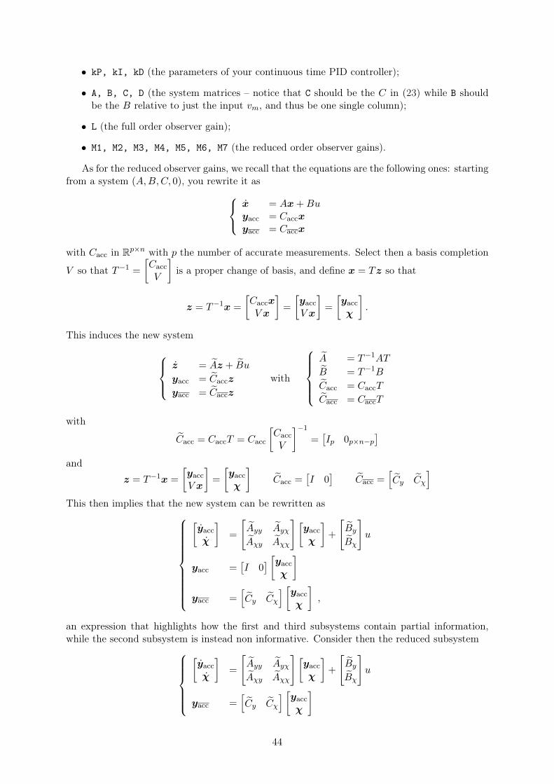
As for the reduced observer gains, we recall that the equations are the following ones: startingfrom a system (A,B,C, 0), you rewrite it as

x = Ax+Buyacc = Caccxyacc = Caccx

with Cacc in Rp×n with p the number of accurate measurements. Select then a basis completion

V so that T−1 =

[CaccV

]is a proper change of basis, and define x = Tz so that

z = T−1x =

[CaccxV x

]=

[yaccV x

]=

[yaccχ

].

This induces the new system

z = Az + Bu

yacc = Caccz

yacc = Caccz

with

A = T−1AT

B = T−1B

Cacc = CaccT

Cacc = CaccT

with

Cacc = CaccT = Cacc

[CaccV

]−1

=[Ip 0p×n−p

]and

z = T−1x =

[yaccV x

]=

[yaccχ

]Cacc =

[I 0

]Cacc =

[Cy Cχ

]This then implies that the new system can be rewritten as

[yaccχ

]=

[Ayy Ayχ

Aχy Aχχ

] [yaccχ

]+

[By

Bχ

]u

yacc =[I 0

] [yaccχ

]yacc =

[Cy Cχ

] [yaccχ

],

an expression that highlights how the first and third subsystems contain partial information,while the second subsystem is instead non informative. Consider then the reduced subsystem

[yaccχ

]=

[Ayy Ayχ

Aχy Aχχ

] [yaccχ

]+

[By

Bχ

]u

yacc =[Cy Cχ

] [yaccχ

]

44

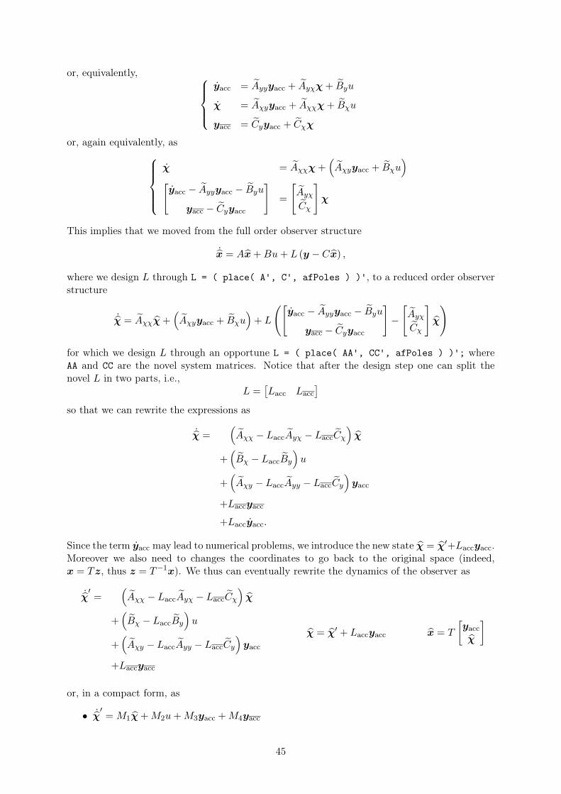
or, equivalently, yacc = Ayyyacc + Ayχχ+ Byu

χ = Aχyyacc + Aχχχ+ Bχu

yacc = Cyyacc + Cχχ

or, again equivalently, asχ = Aχχχ+

(Aχyyacc + Bχu

)[yacc − Ayyyacc − Byu

yacc − Cyyacc

]=

[Ayχ

Cχ

]χ

This implies that we moved from the full order observer structure

˙x = Ax+Bu+ L (y − Cx) ,

where we design L through L = ( place( A', C', afPoles ) )', to a reduced order observerstructure

˙χ = Aχχχ+(Aχyyacc + Bχu

)+ L

([yacc − Ayyyacc − Byu

yacc − Cyyacc

]−

[Ayχ

Cχ

]χ

)

for which we design L through an opportune L = ( place( AA', CC', afPoles ) )'; whereAA and CC are the novel system matrices. Notice that after the design step one can split thenovel L in two parts, i.e.,

L =[Lacc Lacc

]so that we can rewrite the expressions as

˙χ =(Aχχ − LaccAyχ − LaccCχ

)χ

+(Bχ − LaccBy

)u

+(Aχy − LaccAyy − LaccCy

)yacc

+Laccyacc

+Laccyacc.

Since the term yacc may lead to numerical problems, we introduce the new state χ = χ′+Laccyacc.Moreover we also need to changes the coordinates to go back to the original space (indeed,x = Tz, thus z = T−1x). We thus can eventually rewrite the dynamics of the observer as

˙χ′=

(Aχχ − LaccAyχ − LaccCχ

)χ

+(Bχ − LaccBy

)u

+(Aχy − LaccAyy − LaccCy

)yacc

+Laccyacc

χ = χ′ + Laccyacc x = T

[yaccχ

]

or, in a compact form, as

• ˙χ′= M1χ+M2u+M3yacc +M4yacc

45

• χ = χ′ +M5yacc

• x = M6yacc +M7χ.

Reporting 4.8.1 Report:

1. the values of L (the gain of the full order estimator) and M1, . . . ,M7 (the gains of thereduced order estimator);

2. plots of θb, xw and their estimates from both the full and reduced order estimators;

3. the maximum error committed in estimating θb and xw with the full and with the re-duced order observers (thus max

t

∣∣∣θb(t)− θfullb (t)

∣∣∣ and maxt

∣∣∣θb(t)− θreducedb (t)

∣∣∣, and thesame quantities for xw).

46

4.9 Discretize both the controller and observer, and add them to the simu-lator

Reading 4.9

• Section 8.2

• Section 8.3

Before implementing the controller and observer in the Arduino board, we must convert ourcontinuous time strategies into a discrete one and test that we have meaningful results. To thisaim we must perform the following task:

Task 4.9.1

1. discretize the continuous time system (A,B,C, 0) into its discrete equivalent(Ad, Bd, Cd, 0) (you can easily do this in Matlab through the function c2d. Notice thatin the Matlab scripts you will always find the variable fSamplingPeriod – change itsvalue if you want but keep this name!);

2. map the poles for the controller and observer found for the continuous time case throughthe map z = ep∆, where ∆ is the sampling period;

3. compute the gains Kd, Ld, Md1, . . . ,Md7 for the discrete controller and full / reducedobservers using again the functions acker or place (notice that these gains will be differentsince we are in a discrete time case);

4. check that in simulation things still function properly.

To solve the task above follow this procedure:

1. start adding to the Matlab script LabB_ControllerOverSimulator_Discrete_Parameters.mthe value for Kd, stored in the variable Kd. After this, simulate the Simulink diagramLabB_ControllerOverSimulator_Discrete.slx;

2. continue with LabB_ObserverOverSimulator_Discrete_Parameters.m, where you should:

• compute the variables Ad, Bd, Cd and Dd relative to the discretized version of theoriginal system (A,B,C,D);

• compute the variable Ld relative to the gain of the full order discrete observer;

• compute the variables Md1, . . . , Md7 relative to the gains of the reduced order discreteobserver;

• load the gains of your PID controller, i.e., kP, kI and kD.

After this simulate the Simulink diagram LabB_ObserverOverSimulator_Discrete.slx;

3. end with LabB_ObserverAndControllerOverSimulator_Discrete_Parameters.m, whereyou should put all the parameters that you computed in the previous two steps. After this,simulate the Simulink diagram LabB_ObserverAndControllerOverSimulator_Discrete.slx.

47

Important: remember that your actuators saturate at 9 Volts. Thus if you detect that yoursimulated system has a u that is “too big” then you may have problems in the real device. . .

Reporting 4.9.1 Report:

1. how you derived (Ad, Bd, Cd, Dd) and their values;

2. how you derived Kd, Ld, Md1, . . . ,Md7 and their values;

3. a plot of xw, θb and u for the complete control system (controller plus observer).

48

4.10 Test the control strategy with the real robot

Reading 4.10 No readings here!

We are now ready to test the control strategy on the real robot.

Task 4.10.1

1. edit the Matlab script LabB_ObserverAndControllerOverRobot_Parameters.m by addingin it all the variables that you have computed inLabB_ObserverAndControllerOverSimulator_Discrete_Parameters.m;

2. open the Simulink diagram LabB_ObserverAndControllerOverRobot.slx, fix the COMport issue, and explore the diagrams (i.e., how we implemented things). Take special alook at the controller and at the observer, and notice how there are actually 3 differentobservers:

(a) a full order Luenberger observer;

(b) a reduced order Luenberger observer;

(c) a numerical observer, that works by considering all the measurements as accurate,along their numerical derivatives.

It is possible to select which observer you want to use by clicking on the switches;

3. launch different “deploy to hardware” simulations (ctrl+B), and see for which observeryou get the best performance (up to now we instructors got the best performance with thenumerical observer). Of course you can always re-tune the various gains of the controllerand observer in case you are not satisfied with the system – but it is better if you do testson the simulators, before trying on the real robot;

4. to visualize or save the data from the robot follow the same procedure described in Sec-tion 4.4.

Reporting 4.10.1 Report an example of the xw, θb and u obtained with your best controller,and which type of observer you used.

Troubleshooting:

• “my robot does stand upright, but it walks away; it doesn’t go back to the original place!”This may be caused by the drift of the gyro. For example, check Figure 16. θb is estimatedto increase with time, and the robot compensates by actuating opportunely the wheels.The solutions to this problem are two:

– re-tune the gyro, as in Section 4.3;– manually adjust the variable fGyroBias contained in GyroBias.mat, for example by

adding to it the average bias measured in a run where the robot was not disturbed byexternal factors but let walk as it wanted to (something that can be computed usingthe Matlab command

49

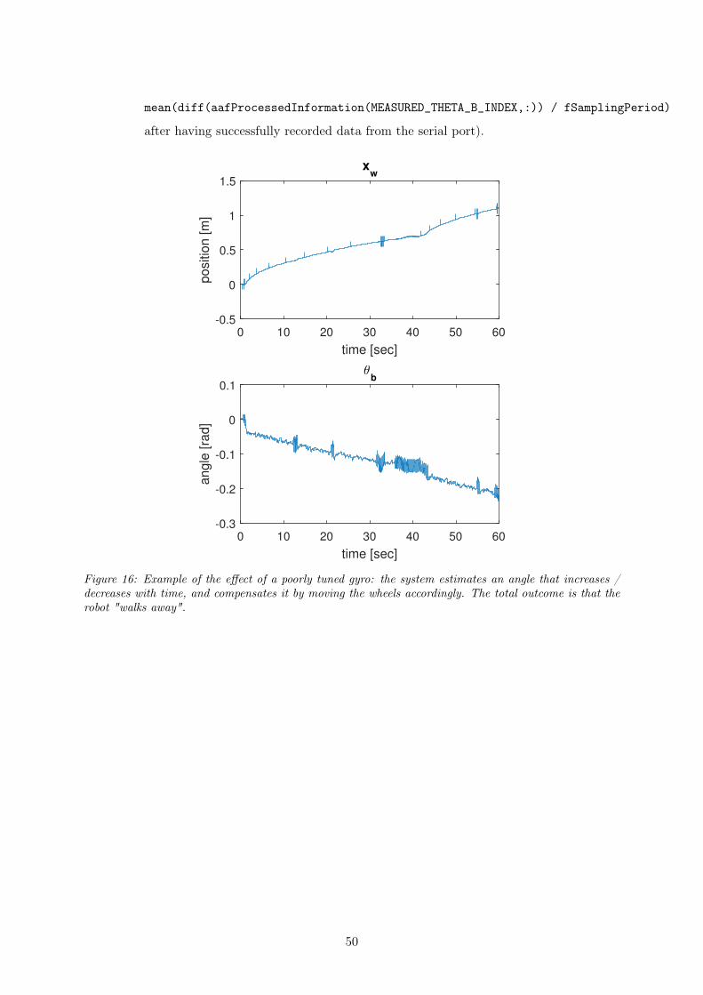
mean(diff(aafProcessedInformation(MEASURED_THETA_B_INDEX,:)) / fSamplingPeriod)

after having successfully recorded data from the serial port).

time [sec]

0 10 20 30 40 50 60

po

sitio

n [m

]

-0.5

0

0.5

1

1.5

xw

time [sec]

0 10 20 30 40 50 60

angle

[ra

d]

-0.3

-0.2

-0.1

0

0.1

θb

Figure 16: Example of the effect of a poorly tuned gyro: the system estimates an angle that increases /decreases with time, and compensates it by moving the wheels accordingly. The total outcome is that therobot "walks away".

50

5 Lab C

The main purpose of this lab is to to re-design the control scheme using directly discrete timeconcepts, and add to the control scheme the management of the reference signal.

5.1 Compute the discrete equivalent of the original model

Reading 5.1

• Section 8.5;

• Section W8.7 (www. fpe7e. com ).

The first part of the following task is equal to Task 4.10.1, thus you basically already solved it.The second no, and you will basically solve it at the end of the lab. Here we will indeed changequite often the used sampling frequency, and test several of them up to the moment where wefind “the best one” (in a sense described better later). You will thus be able to complete thesecond part of this task only at the end of the lab.

Task 5.1.1

1. Discretize the continuous time (A,B,C,D) linear model of the robot and derive its dis-cretized version (Ad, Bd, Cd, Dd) using the sampling period used in Task 4.10.1;

2. find the “best sampling frequency”.

Reporting 5.1.1 Report:

1. the “best sampling frequency” that you found at the end of the lab;

2. the numerical values for (Ad, Bd, Cd, Dd) relative to this sampling period.

5.2 Design the controller using the discrete LQR technique

Reading 5.2

• Section 7.6.2 (being careful that now you are working in discrete-time settings).

This section mimics Section 4.7; here indeed we assume to know the matrix W , indicating how weweight undesirable states, and compute that Kd that minimizes of the discrete time performanceindex

J =+∞∑k=1

ρ[xw(k) xw(k) θb(k) θb(k)

]W

xw(k)xw(k)θb(k)

θb(k)

+ u2(k)

(24)

51

Once again, both W and ρ are design parameters that you can choose. Since you already solvedthis selection in Section 4.7, here we use the same choices of before. Notice that, as before, youwill probably re-do this task several times, one for each sampling period that you will test.

Task 5.2.1

1. start from a sampling frequency of 200Hz, and compute (Ad, Bd, Cd, Dd) as in Section 5.1

2. compute the LQR gain Kd minimizing the cost (24) by using the Matlab function dlqr;

3. insert in the Matlab script LabB_ControllerOverSimulator_Discrete_Parameters.mthe novel value for Kd, stored in the variable Kd, and simulate once again the Simulink di-agram LabB_ControllerOverSimulator_Discrete.slx (i.e., do as you did in Task 4.9.1for testing the controller);

4. if the controller still stabilizes the simulator, reduce the sampling frequency and start over,up to the moment for which the simulated robot falls.

Reporting 5.2.1

1. the sampling frequency for which you lose stability;

2. the corresponding values for Kd and (Ad, Bd, Cd, Dd).

5.3 Design the observer starting from the previously constructed controller

Reading 5.3 No readings here!

Now that Kd is computed, we compute both the full order and the reduced order observers Ld

and Md1, . . . ,Md7. To this aim we directly choose the poles locations wanting the observers tobe from 2 to 6 times faster than the controller poles. Importantly, notice that the concept“faster” is now referred in the discrete time domain. To clarify, in continuous time a polelocated in ps is 5 times slower than a pole located in 5ps. In other words, in continuous timemultiplying times χ implies χ times faster. In discrete time multiplying times χ does not meanχ times faster. For example, if a pole is located in pz = 0.5 (stable), then multiplying times 3leads to something that is unstable.

To understand how to make a pole faster in the discrete domain consider then the followinghint: we know that pz = eps∆, so that

pz = eps∆ ⇒ ps =ln (pz)

∆. (25)

At the same time, if p′z is χ times faster than pz it means that

p′z = ep′s∆ = eχps∆ ⇒ χps =

ln (p′z)

∆⇒ χ

ln (pz)

∆=

ln (p′z)

∆. (26)

From this it is immediate to compute p′z as a function of pz and χ.

52

Task 5.3.1

1. find the formula that describes how to make a discrete pole χ times faster;

2. start again from a sampling frequency of 200Hz, and compute (Ad, Bd, Cd, Dd) as in Sec-tion 5.1

3. choose χ as you did in Task 4.8.1, and compute the gains Kd, Ld, Md1, . . . ,Md7 for thediscrete controller and full / reduced observers (for the reduced order observer you canre-use the equations you used in Task 4.9.1);

4. insert in the Matlab script LabB_ObserverAndControllerOverSimulator_Discrete_Parameters.mthe parameters of the previous controller Kd (corresponding to the right sam-pling time!) and of the current observers and simulate the Simulink diagramLabB_ObserverAndControllerOverSimulator_Discrete.slx;

5. as before, if the controller still stabilizes the simulator, reduce the sampling frequency andstart over, up to the moment for which the simulated robot falls.

Reporting 5.3.1

1. the formula that describes how to make a discrete pole χ times faster;

2. the sampling frequency for which you lose stability;

3. a (brief) discussion on why the critical sampling frequency found now is different fromthat one found in Task 5.2.1;

4. the corresponding values for Kd, Ld, M1d, . . . ,M7d and (Ad, Bd, Cd, Dd).

5.4 Perform experiments on the real balancing robot

Reading 5.4 No readings here!

You have now computed all the information that you already computed in Task 4.9.1, onlyfollowing a different paradigm: instead of starting from a continuous time controller, finding thecontinuous time poles ps, finding the discrete ones through the pz = eps∆ transformation, andthen doing acker on them, you designed directly the pz (and thus an other set of Kd, Ld, andMd1, . . . ,Md7) using discrete time considerations. Here we then repeat some experiments thatare similar to the ones performed in Task 4.10.1, with the aim of checking how different samplingfrequencies affect the real balancing robot.

Task 5.4.1

1. Start from the critical sampling frequency that you computed in Task 5.3.1;

53

2. repeat the same tests you performed in Task 4.10.1 with the new controllers / observers(use the same kind of observer that you used in that task). If the robot does not stabilize,increase the sampling frequency and recompute the various controllers / observers up tothe moment that the robot stabilizes. Save the traces of the xw and θb obtained for thatfrequency (tip: use the serial communications tool, and save the workspace once you havemeaningful result);

3. now increase the sampling frequency 20Hz per time up to the moment you reach 200Hz;for each of these frequencies re-do a balancing experiment, and save each time the xw andθb signals that you obtain.

Reporting 5.4.1

1. the first sampling frequency for which your real robot balances;

2. a graph reporting how the L2 norms of the signals xw and θb depend on the samplingfrequency of the system. Be careful to do not forget that the signals from different experi-ments: a) have different sampling periods; b) may have different durations.

5.5 Design a module for managing external references

Reading 5.5 No readings here!

Among the different possible strategies for managing reference signals, here we choose to imple-ment the ones for which a step in the reference does not excite the state observer. This meansthat the control configuration is as in Figure 17, where the reference enters as a feedforward termso that the poles of the observer are canceled out.

r Nu + sat(·) plant y

−Nx + estimator

−K

Figure 17: Chosen way of introducing the reference input.

The problem is now to compute the values for Nu and Nx that ensure that the DC gain fromr to y is equal to 1. We recall that in continuous time frameworks the formula that guaranteesthis condition is [

Nx

Nu

]=

[A BC D

]−1 [01

](27)

with C here being C = [1 0 0 0], i.e., that C corresponding to measuring xw. Indeed here we areinterested in a reference for changing the x-position of the robot, and not for changing its θb.

54

Shall we then use formula (27) for our discrete time system? No, obviously, since in discretetime settings the condition for guaranteeing a DC gain equal to 1 starts from a different definitionof equilibrium. Indeed for discrete time systems the equilibrium is:

Nxdyss = AdNxdyss +BdNudyssyss = CdNxdyss +DdNudyss.

To derive the formula you can then modify opportunely the computations performed in class.

Task 5.5.1

1. derive the formula for Nx and Nu that guarantees the DC gain from r to y to be 1 fordiscrete time settings;

2. compute Nx and Nu, and put their values in the Matlab scriptLabC_CompensatorOverRobot_Parameters.m, in the variables Nxd and Nud, respec-tively. Notice that this script should also load all the variables computed for solving thetasks above;

3. open the Simulink diagram LabC_CompensatorOverRobot.slx, fix the COM port issue,and explore the block reference inside the block controller. Here you may change yourreference signal as you prefer.

Reporting 5.5.1 Report:

1. the formula for Nx and Nu for the discrete time system, plus the numerical values forthese variables that you obtained applying that formula;

2. the plots of xw, θb, vm and r for some experiments with different reference signals. Inother words, create 2 / 3 different reference signals, and for each of them report how therobots behaves;

3. (optional) compare if your robot behaves better / worse than the robots of your friends.

Notice that the nastier the reference signal is, the more likely your robot is to fall. Youmay consider once again to change the sampling frequency of the whole controller and see if forcertain references signals a certain sampling frequency is not fast enough.

We can thus define as the best sampling frequency the lowest sampling frequencythat makes your robot follow sufficiently safely the nastier reference signal that

you expect it to be required to follow.

Notice that here the definition is deliberately fishy. To define precisely this frequency you mustdefine what is the nastier reference for you. Once you defined it, you can do experiments andsee what is the best frequency for you. And once you did this step, you can eventually completeTask 5.1.1.

55

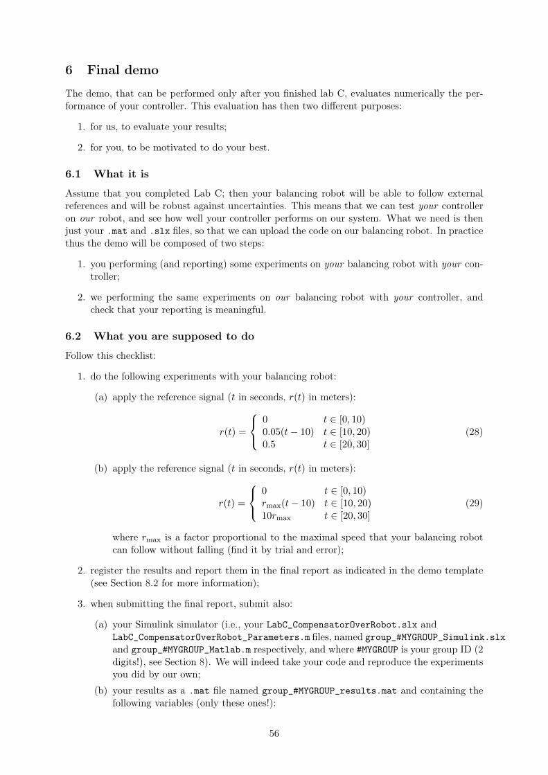
6 Final demo

The demo, that can be performed only after you finished lab C, evaluates numerically the per-formance of your controller. This evaluation has then two different purposes:

1. for us, to evaluate your results;

2. for you, to be motivated to do your best.

6.1 What it is

Assume that you completed Lab C; then your balancing robot will be able to follow externalreferences and will be robust against uncertainties. This means that we can test your controlleron our robot, and see how well your controller performs on our system. What we need is thenjust your .mat and .slx files, so that we can upload the code on our balancing robot. In practicethus the demo will be composed of two steps:

1. you performing (and reporting) some experiments on your balancing robot with your con-troller;

2. we performing the same experiments on our balancing robot with your controller, andcheck that your reporting is meaningful.

6.2 What you are supposed to do

Follow this checklist:

1. do the following experiments with your balancing robot:

(a) apply the reference signal (t in seconds, r(t) in meters):

r(t) =

0 t ∈ [0, 10)0.05(t− 10) t ∈ [10, 20)0.5 t ∈ [20, 30]

(28)

(b) apply the reference signal (t in seconds, r(t) in meters):

r(t) =

0 t ∈ [0, 10)rmax(t− 10) t ∈ [10, 20)10rmax t ∈ [20, 30]

(29)

where rmax is a factor proportional to the maximal speed that your balancing robotcan follow without falling (find it by trial and error);

2. register the results and report them in the final report as indicated in the demo template(see Section 8.2 for more information);

3. when submitting the final report, submit also:

(a) your Simulink simulator (i.e., your LabC_CompensatorOverRobot.slx andLabC_CompensatorOverRobot_Parameters.m files, named group_#MYGROUP_Simulink.slxand group_#MYGROUP_Matlab.m respectively, and where #MYGROUP is your group ID (2digits!), see Section 8). We will indeed take your code and reproduce the experimentsyou did by our own;

(b) your results as a .mat file named group_#MYGROUP_results.mat and containing thefollowing variables (only these ones!):

56

• group_#MYGROUP_experiment_1_times, a column vector containing the samplinginstants of the data relative to r(t) as in Equation (28) (in seconds, and with 0indicating the beginning of the experiment);

• group_#MYGROUP_experiment_1_encoder, a column vector containing the mea-sured xw for the experiment relative to r(t) as in Equation (28) (in meters);

• group_#MYGROUP_experiment_1_angle, a column vector containing the measuredθb for the experiment relative to r(t) as in Equation (28) (in radiants);

• group_#MYGROUP_experiment_1_actuation, a column vector containing the vmsent to the balancing robot’s motor for the experiment relative to r(t) as inEquation (28) (in Volts);

• group_#MYGROUP_experiment_2_times, a column vector containing the samplinginstants of the data relative to r(t) as in Equation (29) (in seconds, and with 0indicating the beginning of the experiment);

• group_#MYGROUP_experiment_2_encoder, a column vector containing the mea-sured xw for the experiment relative to r(t) as in Equation (29) (in meters);

• group_#MYGROUP_experiment_2_angle, a column vector containing the measuredθb for the experiment relative to r(t) as in Equation (29) (in radiants);

• group_#MYGROUP_experiment_2_actuation, a column vector containing the vmsent to the balancing robot’s motor for the experiment relative to r(t) as inEquation (29) (in Volts);

• group_#MYGROUP_r_max, a scalar containing which rmax you found for the exper-iment relative to r(t) as in Equation (29) (in meters / seconds);

• (optional, only if you participate in the International Balancing Robot Race)group_#MYGROUP_r_IRB, a scalar indicating how fast your robot should go in therace.

It is important that you follow the convention for the names indicated above, sincewe process your data in an automatic way.

6.3 How you will be evaluated

The demo is not subject to grading, but follows instead a go / no go concept. Moreprecisely, you get a go when all the following requirements are simultaneously met:

• the results in your group_#MYGROUP_results.mat show that your balancing robot is be-having as we expect it to behave (e.g., be stable, have a sufficiently big rmax, be sufficientlyfast, etc.);

• the data in your group_#MYGROUP_results.mat reproduces the data that we get whenapplying your group_#MYGROUP_Simulink.slx to our unperturbed balancing robot.

6.4 The R7003E 2016 LP2 International Balancing Robot Race

If you are eligible to get bonus points for the labs (i.e., you satisfy the conditions describedin Section 8.3) then you automatically participate to our R7003E 2016 LP2 InternationalBalancing Robot Race!

How does it work?

The race will happen on Monday January 16 2017, 10:00 Central European Time in theControl Engineering Group lab (and everybody is invited). Prior starting the race, we will

57

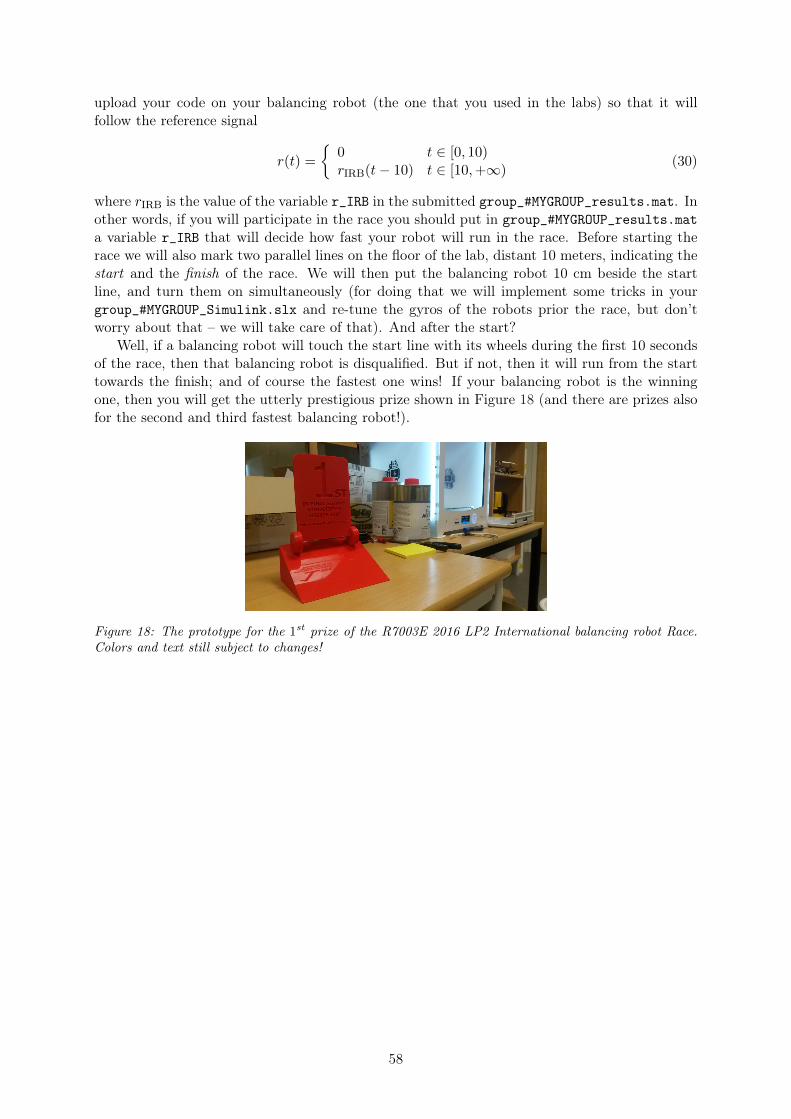
upload your code on your balancing robot (the one that you used in the labs) so that it willfollow the reference signal

r(t) =

{0 t ∈ [0, 10)rIRB(t− 10) t ∈ [10,+∞)

(30)

where rIRB is the value of the variable r_IRB in the submitted group_#MYGROUP_results.mat. Inother words, if you will participate in the race you should put in group_#MYGROUP_results.mata variable r_IRB that will decide how fast your robot will run in the race. Before starting therace we will also mark two parallel lines on the floor of the lab, distant 10 meters, indicating thestart and the finish of the race. We will then put the balancing robot 10 cm beside the startline, and turn them on simultaneously (for doing that we will implement some tricks in yourgroup_#MYGROUP_Simulink.slx and re-tune the gyros of the robots prior the race, but don’tworry about that – we will take care of that). And after the start?

Well, if a balancing robot will touch the start line with its wheels during the first 10 secondsof the race, then that balancing robot is disqualified. But if not, then it will run from the starttowards the finish; and of course the fastest one wins! If your balancing robot is the winningone, then you will get the utterly prestigious prize shown in Figure 18 (and there are prizes alsofor the second and third fastest balancing robot!).

Figure 18: The prototype for the 1st prize of the R7003E 2016 LP2 International balancing robot Race.Colors and text still subject to changes!

58

7 Optional tasks

If you had fun up to now, then you may want to do also some other tasks (that are not justvery fun to do, but that also lead to learning very useful skills). Notice: no additional points forcompleting these tasks, but we ensure you that you will get a lot of gratification. Some of theadditional tasks are actually quite hard; in case you are interested we can make them become aMaster Thesis project.

• make the balancing robot start moving only when “poked”;

• make the balancing robot stop moving when “poked” once again;

• add an other motor to the balancing robot, and add the possibility of steering it;

• visualize the motion of the balancing robot through our Vicon MoCap system;

• write a phone app so that you get the data from the balancing robot via Bluetooth;

• write a phone app so that you can draw a path in your phone and make the robot followit;

• add a camera to the balancing robot and make it an exploring balancing robot.

59

8 Reporting your findings

Important: every group will have an ID number that is composed by two digits. In otherwords, the first group will have the ID number 01, the second 02, etc. This means that, forexample, the Simulink file submitted by the first group is group_01_Simulink.slx (and notgroup_1_Simulink.slx!). Moreover, we are case sensitive, in the sense that for us Group_01_Simulink.slxis very different from group_01_Simulink.slx. Same for the reports. Clear?

8.1 The labs reports

8.1.1 What they are

They are very brief documents that you compile by group (thus one report for each group) andthat you upload in Canvas. We will use these documents not primarily to evaluate you, butrather to give you feedback on how you are doing. It should not take too much time to compilethem (specially if you automate the production of the figures).

8.1.2 What you are supposed to do

For every report (A, B or C), follow this checklist:

1. download the corresponding template from http://staff.www.ltu.se/~damvar/R7003E-2016-LP2.html;

2. compile the templates following the instructions that they contain;

3. name the compiled template as group_#MYGROUP_lab_#LAB.pdf, with #MYGROUP being yourtwo digits group code, and #LAB being either A, B or C, accordingly;

4. upload the template in Canvas (notice that it is the first time that we teachers are usingCanvas so we have still to understand how this works; nonetheless we will solve this issuesoon and inform accordingly).

Important: the reports must be in a .pdf format. If you do things in Word or stuff likethat then export your file in a .pdf. We will not evaluate reports that are not in a .pdf format.Thus “no .pdf” =⇒ failing the lab.

8.1.3 How you will be evaluated

First of all, every report should be complete: we will not evaluate documents that miss reportingthings that have been asked to be reported. Second, reports should comply with the giventemplate. For example, if the maximum number of pages allowed is 6, then you have to submita document that is at most 6 pages. Once complete and complying with the requirements inthe templates, reports will be evaluated by us and graded with a number ranging from 0 (worstpossible) to 100 (best possible), with 60 indicating the sufficiency. If you get an insufficiency insome report then you will have to improve it up to the moment that you get a grading ≥ 60.

Every lab report will be evaluated independently following these performance metrics:

correctness of the results, for a total of 50 points (0 = nothing is correct, 50 = no mistakesin the derivations, in the block schemes, etc.);

analysis of the results, for a total of 50 points (0 = you analyzed nothing, 50 = you analyzedeverything and correctly). Despite the lab reports will not require too much analysis, therewill be some questions that challenge your knowledge. Your analysis is meant to be inthis way: you obtain a specific result (for example, the PID controller behaves better insimulation than in reality). Then, why do you think you got that specific result? What does

60

it say to you? What are the implications? Analyzing a result is a difficult task, and wewant you to feel free to discuss what you find however you want. But the caveat is: wewant to understand if you understood, and not see what you did. In other words, saying“we did this this and this and the result is shown in figure 7” is not an analysis. Instead, weprefer something like “we did this, and found that the system behaves in this way; initiallywe thought that it was because of this, but then we did this other experiment and foundthat. So we feel like this is happening, because of this this and this other reason”. Noticethat it is completely ok to say that you did not understand something / you do notknow why something else is happening; but show us that you tried thinking at what youdid, and not that you just monkey-made the labs.

8.2 The final report

8.2.1 What it is

It is a document that you send us via Canvas, and that is used not just to evaluate you, but alsoto train you writing scientific articles.

8.2.2 What you are supposed to do

Follow this checklist:

1. download the corresponding template from http://staff.www.ltu.se/~damvar/R7003E-2016-LP2.html;

2. compile it following the hints that it contains. Notice that what you are supposedto put inside the manuscript is not just a condensation of the three labs, but rather anexercise on how to write academic papers;

3. name the compiled template as group_#MYGROUP_final_report.pdf, with #MYGROUP beingyour two digits group code;

4. upload it in Canvas.

Important (en gång till): the reports must be in a .pdf format. If you do things in Wordor stuff like that then export your file in a .pdf. We will not evaluate reports that are not in a.pdf format.

8.2.3 How you will be evaluated

Like as in Section 8.1.3, plus an eye for your capacity of understanding what is important andwhat is not. Notice that the final report will contain information on your experiments for thedemo.

8.3 Bonus points

If, simultaneously:

• you are taking the course in 2016 LP2;

• respect all the following deadlines:

1. submit the report for lab A before Tuesday November 29 2016, 14:45 Central EuropeanTime;

2. submit the report for lab B before Tuesday December 13 2016, 14:45 Central EuropeanTime;

61

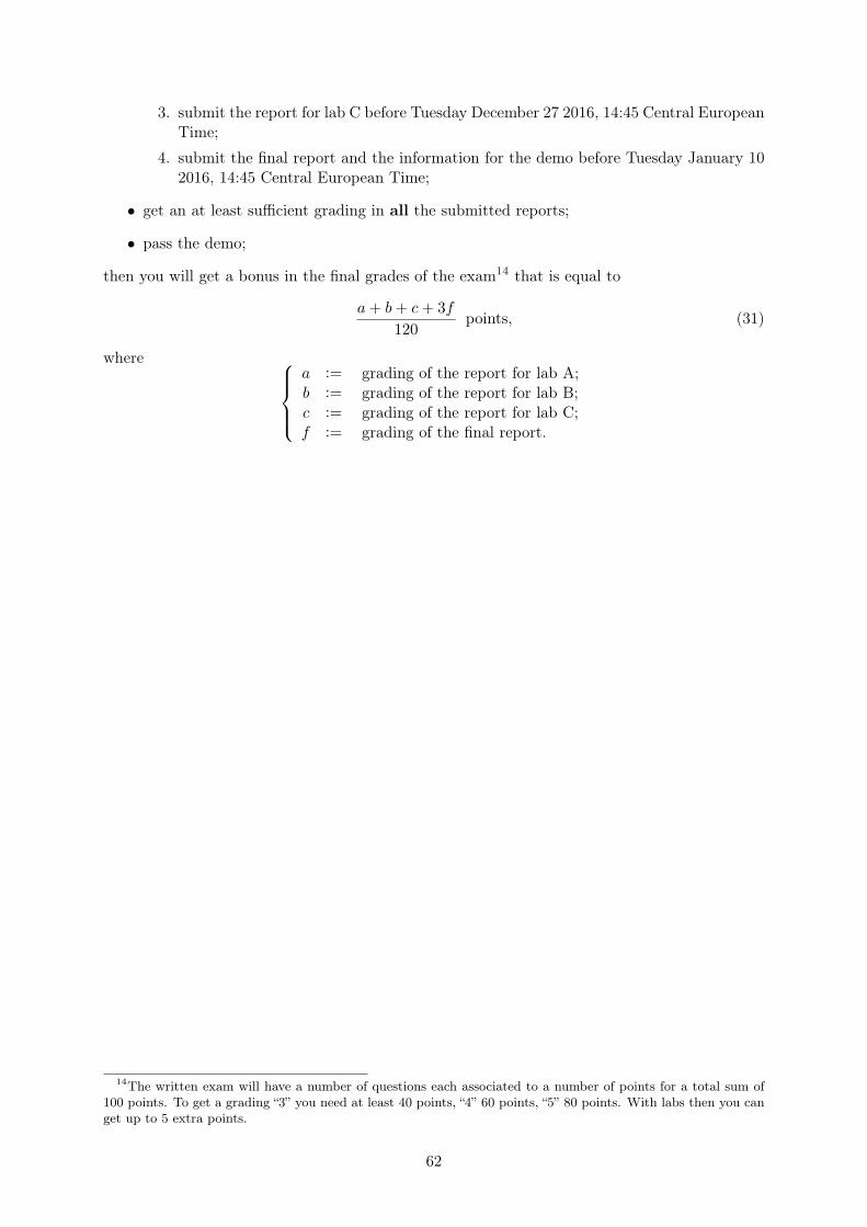
3. submit the report for lab C before Tuesday December 27 2016, 14:45 Central EuropeanTime;

4. submit the final report and the information for the demo before Tuesday January 102016, 14:45 Central European Time;

• get an at least sufficient grading in all the submitted reports;

• pass the demo;

then you will get a bonus in the final grades of the exam14 that is equal to

a+ b+ c+ 3f

120points, (31)

where a := grading of the report for lab A;b := grading of the report for lab B;c := grading of the report for lab C;f := grading of the final report.

14The written exam will have a number of questions each associated to a number of points for a total sum of100 points. To get a grading “3” you need at least 40 points, “4” 60 points, “5” 80 points. With labs then you canget up to 5 extra points.

62

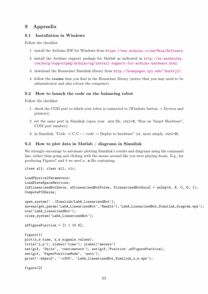
9 Appendix

9.1 Installation in Windows

Follow the checklist:

1. install the Arduino IDE for Windows from https://www.arduino.cc/en/Main/Software;

2. install the Arduino support package for Matlab as indicated in http://se.mathworks.com/help/supportpkg/arduino/ug/install-support-for-arduino-hardware.html;

3. download the Rensselaer Simulink library from http://homepages.rpi.edu/~hurstj2/;

4. follow the readme that you find in the Rensselaer library (notice that you may need to beadministrator and also reboot the computer).

9.2 How to launch the code on the balancing robot

Follow the checklist:

1. check the COM port to which your robot is connected to (Windows button → Devices andprinters);

2. set the same port in Simulink (open your .slx file, ctrl+E, “Run on Target Hardware”,COM port number);

3. in Simulink, “Code → C/C++ code → Deploy to hardware” (or, more simply, ctrl+B).

9.3 How to plot data in Matlab / diagrams in Simulink

We strongly encourage to automate plotting Simulink’s results and diagrams using the commandline, rather than going and clicking with the mouse around like you were playing doom. E.g., forproducing Figures7 and 8 we used a .m file containing:

close all; clear all; clc;

LoadPhysicalParameters;LoadStateSpaceMatrices;[afLinearizedBotZeros, afLinearizedBotPoles, fLinearizedBotGain] = ss2zp(A, B, C, D, 1);ComputePIDGains;

open_system('../Simulink/LabA_LinearizedBot');saveas(get_param('LabA_LinearizedBot','Handle'),'LabA_LinearizedBot_Simulink_diagram.eps');sim('LabA_LinearizedBot');close_system('LabA_LinearizedBot');

afFigurePosition = [1 1 10 6];

figure(1)plot(x_w.time, x_w.signals.values);title('x_w'); xlabel('time'); ylabel('meters')set(gcf, 'Units', 'centimeters'); set(gcf,'Position',afFigurePosition);set(gcf, 'PaperPositionMode', 'auto');print('-depsc2', '-r300', 'LabA_LinearizedBot_Simulink_x_w.eps');

figure(2)

63

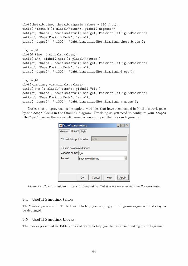
plot(theta_b.time, theta_b.signals.values * 180 / pi);title('\theta_b'); xlabel('time'); ylabel('degrees')set(gcf, 'Units', 'centimeters'); set(gcf,'Position',afFigurePosition);set(gcf, 'PaperPositionMode', 'auto');print('-depsc2', '-r300', 'LabA_LinearizedBot_Simulink_theta_b.eps');

figure(3)plot(d.time, d.signals.values);title('d'); xlabel('time'); ylabel('Newton')set(gcf, 'Units', 'centimeters'); set(gcf,'Position',afFigurePosition);set(gcf, 'PaperPositionMode', 'auto');print('-depsc2', '-r300', 'LabA_LinearizedBot_Simulink_d.eps');

figure(4)plot(v_m.time, v_m.signals.values);title('v_m'); xlabel('time'); ylabel('Volt')set(gcf, 'Units', 'centimeters'); set(gcf,'Position',afFigurePosition);set(gcf, 'PaperPositionMode', 'auto');print('-depsc2', '-r300', 'LabA_LinearizedBot_Simulink_v_m.eps');

Notice that the previous .m file exploits variables that have been loaded in Matlab’s workspaceby the scope blocks in the Simulink diagram. For doing so you need to configure your scopes(the “gear” icon in the upper left corner when you open them) as in Figure 19.

Figure 19: How to configure a scope in Simulink so that it will save your data on the workspace.

9.4 Useful Simulink tricks

The “tricks” presented in Table 1 want to help you keeping your diagrams organized and easy tobe debugged.

9.5 Useful Simulink blocks

The blocks presented in Table 2 instead want to help you be faster in creating your diagrams.

64

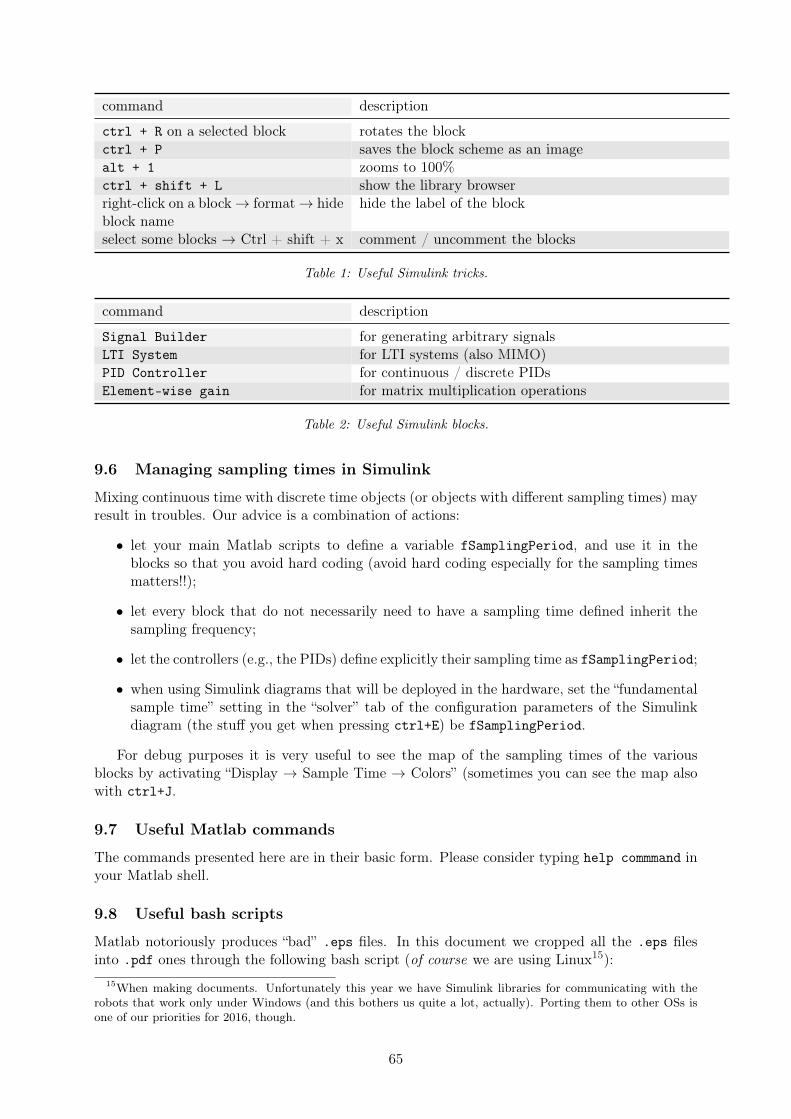
command description

ctrl + R on a selected block rotates the blockctrl + P saves the block scheme as an imagealt + 1 zooms to 100%ctrl + shift + L show the library browserright-click on a block → format → hideblock name

hide the label of the block

select some blocks → Ctrl + shift + x comment / uncomment the blocks

Table 1: Useful Simulink tricks.

command description

Signal Builder for generating arbitrary signalsLTI System for LTI systems (also MIMO)PID Controller for continuous / discrete PIDsElement-wise gain for matrix multiplication operations

Table 2: Useful Simulink blocks.

9.6 Managing sampling times in Simulink

Mixing continuous time with discrete time objects (or objects with different sampling times) mayresult in troubles. Our advice is a combination of actions:

• let your main Matlab scripts to define a variable fSamplingPeriod, and use it in theblocks so that you avoid hard coding (avoid hard coding especially for the sampling timesmatters!!);

• let every block that do not necessarily need to have a sampling time defined inherit thesampling frequency;

• let the controllers (e.g., the PIDs) define explicitly their sampling time as fSamplingPeriod;

• when using Simulink diagrams that will be deployed in the hardware, set the “fundamentalsample time” setting in the “solver” tab of the configuration parameters of the Simulinkdiagram (the stuff you get when pressing ctrl+E) be fSamplingPeriod.

For debug purposes it is very useful to see the map of the sampling times of the variousblocks by activating “Display → Sample Time → Colors” (sometimes you can see the map alsowith ctrl+J.

9.7 Useful Matlab commands

The commands presented here are in their basic form. Please consider typing help commmand inyour Matlab shell.

9.8 Useful bash scripts

Matlab notoriously produces “bad” .eps files. In this document we cropped all the .eps filesinto .pdf ones through the following bash script (of course we are using Linux15):

15When making documents. Unfortunately this year we have Simulink libraries for communicating with therobots that work only under Windows (and this bothers us quite a lot, actually). Porting them to other OSs isone of our priorities for 2016, though.

65

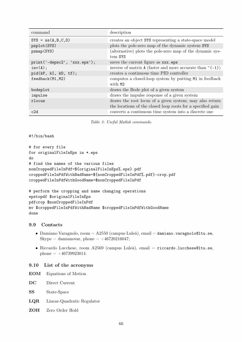
command description

SYS = ss(A,B,C,D) creates an object SYS representing a state-space modelpzplot(SYS) plots the pole-zero map of the dynamic system SYSpzmap(SYS) (alternative) plots the pole-zero map of the dynamic sys-

tem SYSprint('-depsc2', 'xxx.eps'); saves the current figure as xxx.epsinv(A); inverse of matrix A (faster and more accurate than ^(-1))pid(kP, kI, kD, tf); creates a continuous time PID controllerfeedback(M1,M2) computes a closed-loop system by putting M1 in feedback

with M2bodeplot draws the Bode plot of a given systemimpulse draws the impulse response of a given systemrlocus draws the root locus of a given system; may also return

the locations of the closed loop roots for a specified gainc2d converts a continuous time system into a discrete one

Table 3: Useful Matlab commands.

#!/bin/bash

# for every filefor originalFileInEps in *.epsdo# find the names of the various filesnonCroppedFileInPdf=${originalFileInEps%.eps}.pdfcroppedFileInPdfWithBadName=${nonCroppedFileInPdf%.pdf}-crop.pdfcroppedFileInPdfWithGoodName=$nonCroppedFileInPdf

# perform the cropping and name changing operationsepstopdf $originalFileInEpspdfcrop $nonCroppedFileInPdfmv $croppedFileInPdfWithBadName $croppedFileInPdfWithGoodNamedone

9.9 Contacts

• Damiano Varagnolo, room = A2550 (campus Luleå), email = damiano.varagnolo@ltu.se,Skype = damianovar, phone = +46720216047;

• Riccardo Lucchese, room A2569 (campus Luleå), email = riccardo.lucchese@ltu.se,phone = +46739923014.

9.10 List of the acronyms

EOM Equations of Motion

DC Direct Current

SS State-Space

LQR Linear-Quadratic Regulator

ZOH Zero Order Hold

66

SRL Symmetric Root Locus

MIMO Multi Input Multi Output

67

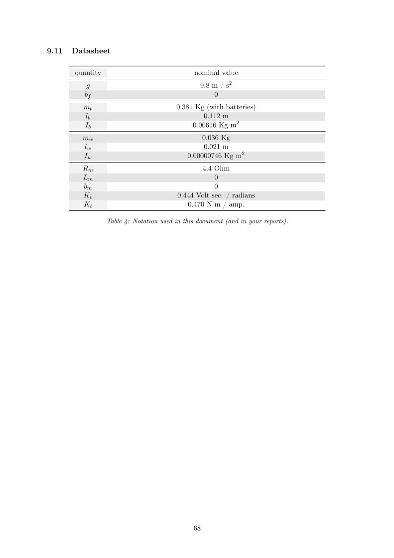
9.11 Datasheet

quantity nominal value

g 9.8 m / s2

bf 0

mb 0.381 Kg (with batteries)lb 0.112 mIb 0.00616 Kg m2

mw 0.036 Kglw 0.021 mIw 0.00000746 Kg m2

Rm 4.4 OhmLm 0bm 0Ke 0.444 Volt sec. / radiansKt 0.470 N m / amp.

Table 4: Notation used in this document (and in your reports).

68

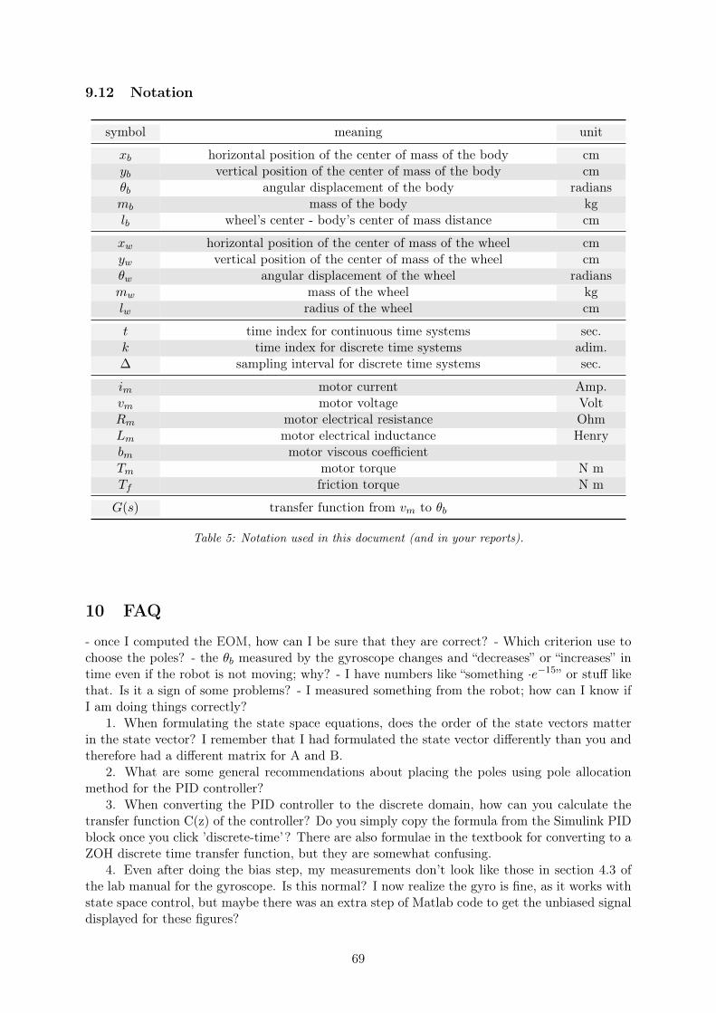
9.12 Notation

symbol meaning unit

xb horizontal position of the center of mass of the body cmyb vertical position of the center of mass of the body cmθb angular displacement of the body radiansmb mass of the body kglb wheel’s center - body’s center of mass distance cm

xw horizontal position of the center of mass of the wheel cmyw vertical position of the center of mass of the wheel cmθw angular displacement of the wheel radiansmw mass of the wheel kglw radius of the wheel cm

t time index for continuous time systems sec.k time index for discrete time systems adim.∆ sampling interval for discrete time systems sec.

im motor current Amp.vm motor voltage VoltRm motor electrical resistance OhmLm motor electrical inductance Henrybm motor viscous coefficientTm motor torque N mTf friction torque N m

G(s) transfer function from vm to θb

Table 5: Notation used in this document (and in your reports).

10 FAQ

- once I computed the EOM, how can I be sure that they are correct? - Which criterion use tochoose the poles? - the θb measured by the gyroscope changes and “decreases” or “increases” intime even if the robot is not moving; why? - I have numbers like “something ·e−15” or stuff likethat. Is it a sign of some problems? - I measured something from the robot; how can I know ifI am doing things correctly?

1. When formulating the state space equations, does the order of the state vectors matterin the state vector? I remember that I had formulated the state vector differently than you andtherefore had a different matrix for A and B.

2. What are some general recommendations about placing the poles using pole allocationmethod for the PID controller?

3. When converting the PID controller to the discrete domain, how can you calculate thetransfer function C(z) of the controller? Do you simply copy the formula from the Simulink PIDblock once you click ’discrete-time’? There are also formulae in the textbook for converting to aZOH discrete time transfer function, but they are somewhat confusing.

4. Even after doing the bias step, my measurements don’t look like those in section 4.3 ofthe lab manual for the gyroscope. Is this normal? I now realize the gyro is fine, as it works withstate space control, but maybe there was an extra step of Matlab code to get the unbiased signaldisplayed for these figures?

69

5. Should you expect your PID to be able to balance the robot for close to 10 seconds? Inow realize it’s possible, but not without a lot of manual tuning.

1. The gain, check negative feedback. 2. The Nyquist plots. We had a bit of trubbleunderstaning our resulting Nyquist plot and what we where supposed to expect. 3. In retrospectwe might have had needed some intuition on how the matrices A,B,C and D relates to the EOMsso that we could see if we have the correct equations or not. Perheps where to expect values andwhere not to. 3. The pole allocation method. One tip we found usefull and helped us was to doit symbolically. 4. Tips and/or pointers on how one can determine the gain, K-value.

70