Binomial, Multinomial & Poisson · 2012-08-31 · Multinomial Distribution •Series of n...
36
Binomial, Multinomial & Poisson Stat 557 Fall 2012
Transcript of Binomial, Multinomial & Poisson · 2012-08-31 · Multinomial Distribution •Series of n...
Binomial, Multinomial & Poisson
Stat 557Fall 2012
Outline
• Coverage of C.I for π
• Multinomial
• Poisson
• Sampling Types
• Contingency Tables
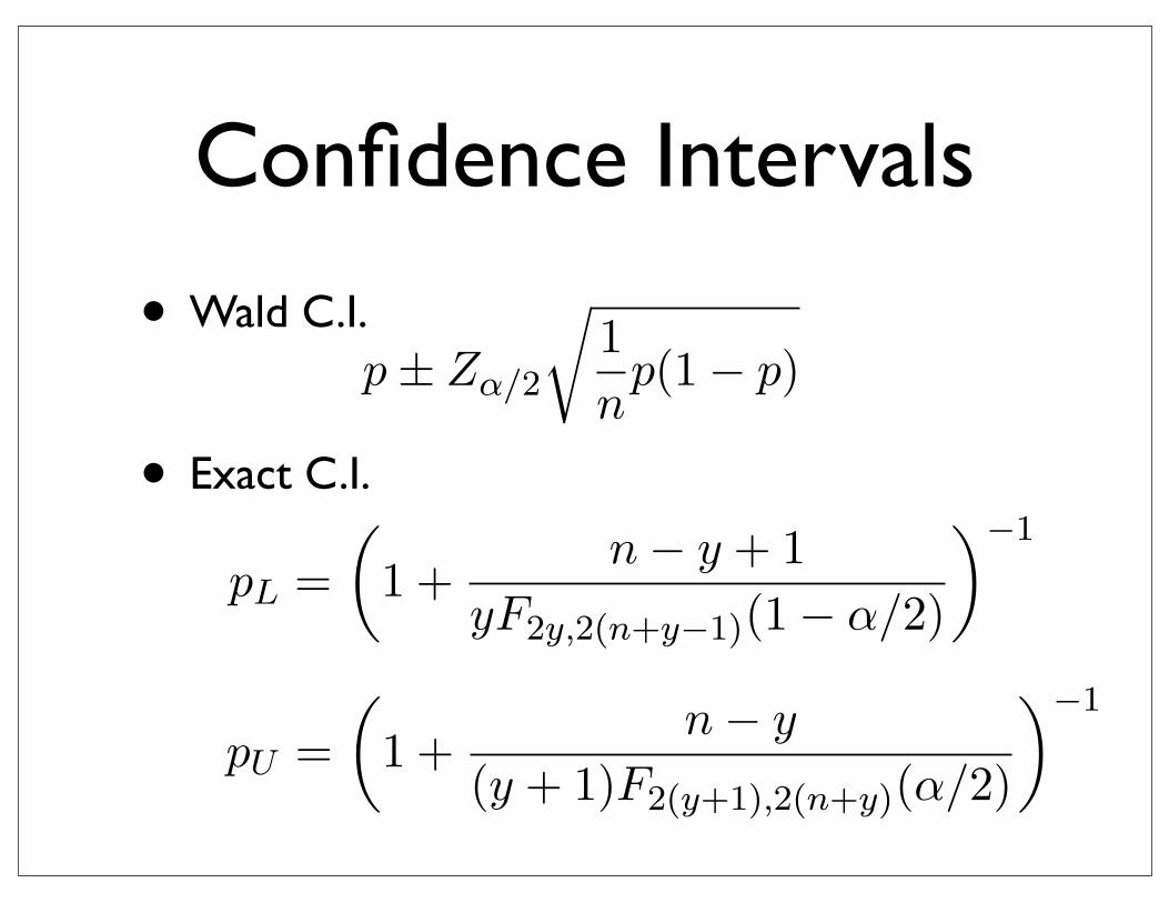
Confidence Intervals
• Wald C.I.
• Exact C.I.
α
2= P (Y ≥ y) =
n�
j=y
�n
j
�pj(1− p)n−j
α
2= P (Y ≤ y) =
y�
j=0
�n
j
�pj(1− p)n−j
pL =�
1 +n− y + 1
yF2y,2(n+y−1)(1− α/2)
�−1
pU =�
1 +n− y
(y + 1)F2(y+1),2(n+y)(α/2)
�−1
C(p, n) =n�
j=0
I(j, p) ·�
n
j
�pj(1− p)n−j
M ≤ 1.96 ·�
1n
p(1− p)
n ≥Z2
α/2
Mp(1− p)
6
α
2= P (Y ≥ y) =
n�
j=y
�n
j
�pj(1− p)n−j
α
2= P (Y ≤ y) =
y�
j=0
�n
j
�pj(1− p)n−j
pL =�
1 +n− y + 1
yF2y,2(n+y−1)(1− α/2)
�−1
pU =�
1 +n− y
(y + 1)F2(y+1),2(n+y)(α/2)
�−1
C(p, n) =n�
j=0
I(j, p) ·�
n
j
�pj(1− p)n−j
M ≤ 1.96 ·�
1n
p(1− p)
n ≥Z2
α/2
Mp(1− p)
6
|p− π|�1nπ(1− π)
.∼ N(0, 1)
nπ ≥ 5, n(1− π) ≥ 5
|p− π|�1np(1− p)
< Zα/2
pU = p + Zα/2
�1n
p(1− p)
pL = p− Zα/2
�1n
p(1− p)
α = 0.05α/2 = 0.025
Zα/2 = 1.96n = 115
p = 0.6 =69115
pL = 0.6− 1.96 ·�
0.6 · 0.4115
=
= 0.6− 0.0895 = 0.5105
pU = 0.6 + 1.96 ·�
0.6 · 0.4115
=
= 0.6 + 0.0895 = 0.6895
p ± Zα/2
�1n
p(1− p)
P (Y ≤ y) =α
2
5
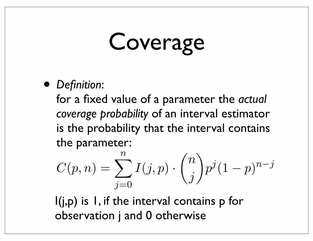
Coverage
• Definition: for a fixed value of a parameter the actual coverage probability of an interval estimator is the probability that the interval contains the parameter:
I(j,p) is 1, if the interval contains p for observation j and 0 otherwise
α
2= P (Y ≥ y) =
n�
j=y
�n
j
�pj(1− p)n−j
α
2= P (Y ≤ y) =
y�
j=0
�n
j
�pj(1− p)n−j
pL =�
1 +n− y + 1
yF2y,2(n+y−1)(1− α/2)
�−1
pU =�
1 +n− y
(y + 1)F2(y+1),2(n+y)(α/2)
�−1
C(p, n) =n�
j=0
I(j, p) ·�
n
j
�pj(1− p)n−j
M ≤ 1.96 ·�
1n
p(1− p)
n ≥Z2
α/2
Mp(1− p)
6
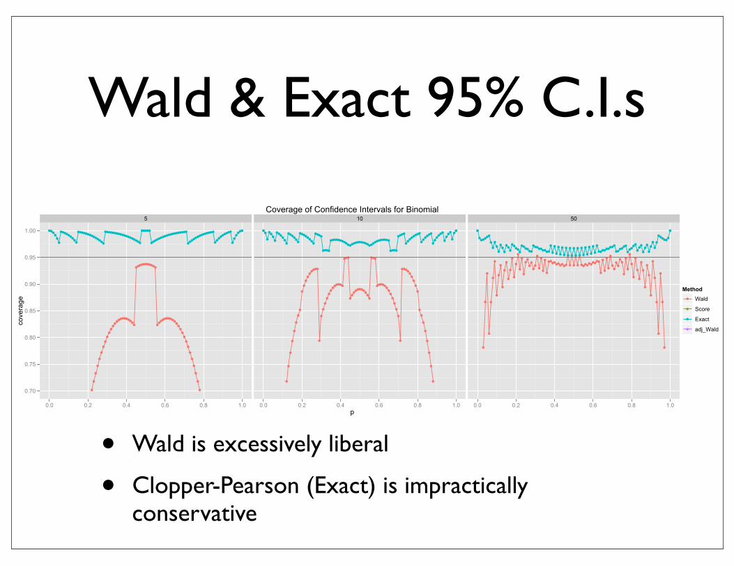
Wald & Exact 95% C.I.s
• Wald is excessively liberal
• Clopper-Pearson (Exact) is impractically conservative
Coverage of Confidence Intervals for Binomial
p
coverage
0.70
0.75
0.80
0.85
0.90
0.95
1.00
5
0.0 0.2 0.4 0.6 0.8 1.0
10
0.0 0.2 0.4 0.6 0.8 1.0
50
0.0 0.2 0.4 0.6 0.8 1.0
Method
Wald
Score
Exact
adj_Wald
Score
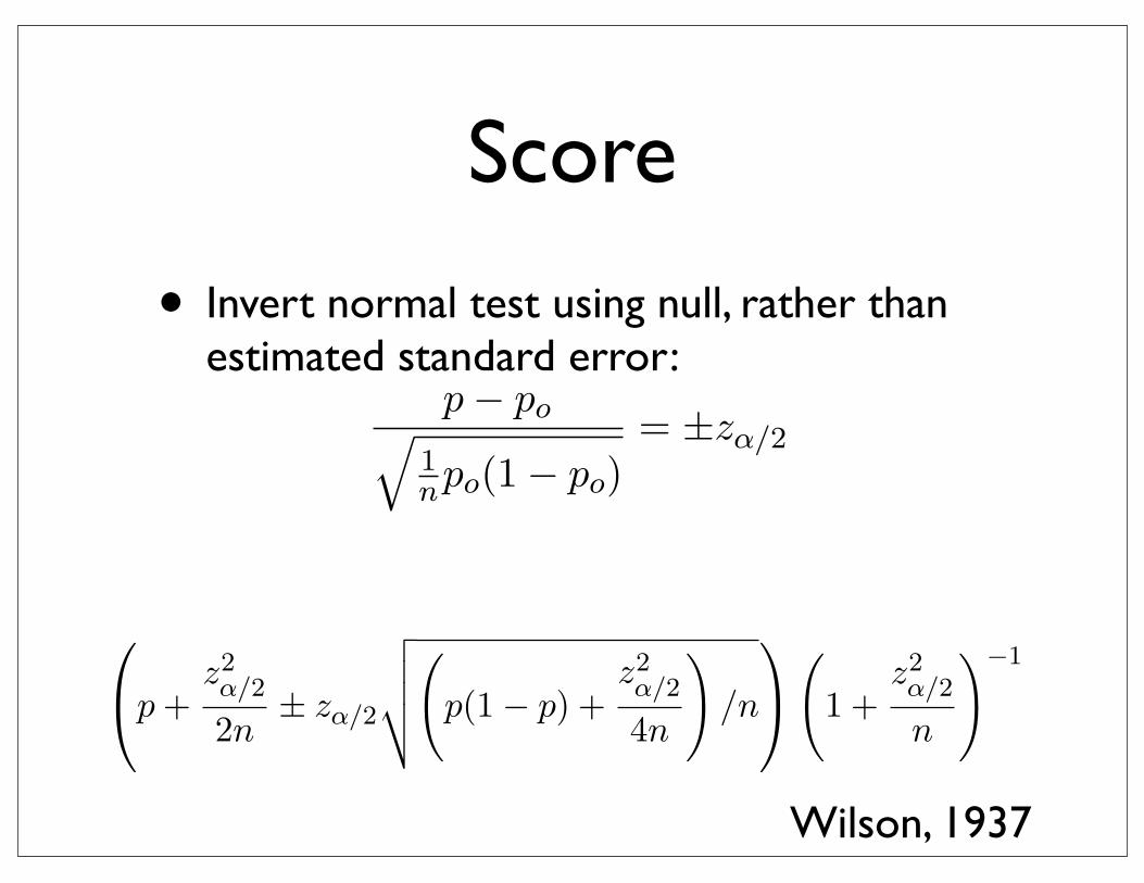
• Invert normal test using null, rather than estimated standard error:
p− po�1npo(1− po
= ±zα/2
p +z2α/2
2n± zα/2
�����
p(1− p) +z2α/2
4n
�/n
�
1 +z2α/2
n
�−1
p =Y
n
|p− π|�1np(1− p)
.∼ N(0, 1)
nπ ≥ 5, n(1− π) ≥ 5
λ ·��
β2 +�
α2�
{α0m, αm : m = 1, ...,M} M(p + 1){β0k, βk : k = 1, ...,K} K(M + 1)
gk(T ) =eTk
�K�=1 eT�
σ(ν) =1
1 + e−ν
Zm = σ(α0m + α�mX) m = 1, ...,M
Tk = β0k + β�kZ k = 1, ...,K
fk(X) = gk(T ) k = 1, ...,K
Πc = 2I�
i=1
J�
j=1
πij ·�
h>i
�
k>j
πhk =�
i,j
πcij
σ2(γ̂)∞ =16
n(ΠC + ΠD)4
I�
i=1
J�
j=1
πij
�ΠCπd
ij −ΠDπcij
�2
1
p̃ =y + 2n + 4
p̃ ± zα/2
�1n
p̃(1− p̃)
p− po�1npo(1− po)
= ±zα/2
p +z2α/2
2n± zα/2
�����
p(1− p) +z2α/2
4n
�/n
�
1 +z2α/2
n
�−1
p =Y
n
|p− π|�1np(1− p)
.∼ N(0, 1)
nπ ≥ 5, n(1− π) ≥ 5
λ ·��
β2 +�
α2�
{α0m, αm : m = 1, ...,M} M(p + 1){β0k, βk : k = 1, ...,K} K(M + 1)
gk(T ) =eTk
�K�=1 eT�
σ(ν) =1
1 + e−ν
Zm = σ(α0m + α�mX) m = 1, ...,M
Tk = β0k + β�kZ k = 1, ...,K
fk(X) = gk(T ) k = 1, ...,K
Πc = 2I�
i=1
J�
j=1
πij ·�
h>i
�
k>j
πhk =�
i,j
πcij
1
Wilson, 1937
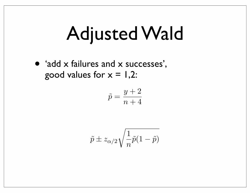
Adjusted Wald
• ‘add x failures and x successes’, good values for x = 1,2:
p̃ =y + 2n + 4
p̃ + zα/2
�1n
p̃(1− p̃)
p− po�1npo(1− po
= ±zα/2
p +z2α/2
2n± zα/2
�����
p(1− p) +z2α/2
4n
�/n
�
1 +z2α/2
n
�−1
p =Y
n
|p− π|�1np(1− p)
.∼ N(0, 1)
nπ ≥ 5, n(1− π) ≥ 5
λ ·��
β2 +�
α2�
{α0m, αm : m = 1, ...,M} M(p + 1){β0k, βk : k = 1, ...,K} K(M + 1)
gk(T ) =eTk
�K�=1 eT�
σ(ν) =1
1 + e−ν
Zm = σ(α0m + α�mX) m = 1, ...,M
Tk = β0k + β�kZ k = 1, ...,K
fk(X) = gk(T ) k = 1, ...,K
Πc = 2I�
i=1
J�
j=1
πij ·�
h>i
�
k>j
πhk =�
i,j
πcij
1
p̃ =y + 2n + 4
p̃ ± zα/2
�1n
p̃(1− p̃)
p− po�1npo(1− po
= ±zα/2
p +z2α/2
2n± zα/2
�����
p(1− p) +z2α/2
4n
�/n
�
1 +z2α/2
n
�−1
p =Y
n
|p− π|�1np(1− p)
.∼ N(0, 1)
nπ ≥ 5, n(1− π) ≥ 5
λ ·��
β2 +�
α2�
{α0m, αm : m = 1, ...,M} M(p + 1){β0k, βk : k = 1, ...,K} K(M + 1)
gk(T ) =eTk
�K�=1 eT�
σ(ν) =1
1 + e−ν
Zm = σ(α0m + α�mX) m = 1, ...,M
Tk = β0k + β�kZ k = 1, ...,K
fk(X) = gk(T ) k = 1, ...,K
Πc = 2I�
i=1
J�
j=1
πij ·�
h>i
�
k>j
πhk =�
i,j
πcij
1
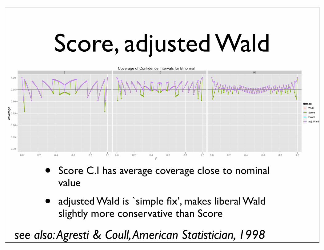
Score, adjusted Wald
• Score C.I has average coverage close to nominal value
• adjusted Wald is `simple fix’, makes liberal Wald slightly more conservative than Score
Coverage of Confidence Intervals for Binomial
p
coverage
0.70
0.75
0.80
0.85
0.90
0.95
1.00
5
0.0 0.2 0.4 0.6 0.8 1.0
10
0.0 0.2 0.4 0.6 0.8 1.0
50
0.0 0.2 0.4 0.6 0.8 1.0
Method
Wald
Score
Exact
adj_Wald
see also: Agresti & Coull, American Statistician, 1998
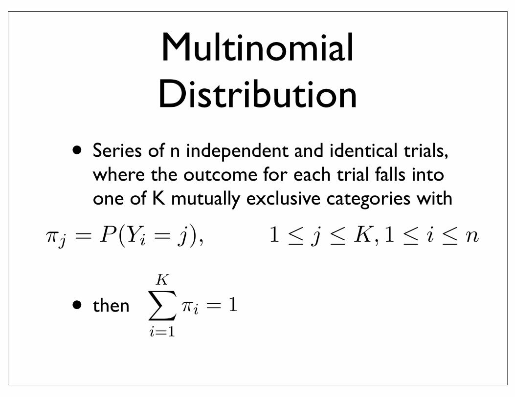
Multinomial Distribution
• Series of n independent and identical trials, where the outcome for each trial falls into one of K mutually exclusive categories with
• then
is called a two dimensional contingency table or cross-classification table. If πij denotesthe probability of pair (xi, yj) then the table
X\Y y1 y2 ... yJ
x1 π11 π12 ... π1J π1.
x2 π21 π22 ... π2J π2....
...... . . . ...
...xI πI1 πI2 ... πIJ πI.
π.1 π.2 ... π.J 1
contains the joint distribution and {π1., π2., ...,πI.} and {π.1, π.2, ...,π.J} are marginal dis-tributions.
G2 = 2
�
i
yi log�
mi
m0,i
�= 0.74
X2 =
�
i
(mi −m0,i)2
m0,i= 0.69
Ha : 0 ≤ π ≤ 1 with π1 + π2 + π3 = 1
Ho : π = πo
πo =
0.750.18750.0625
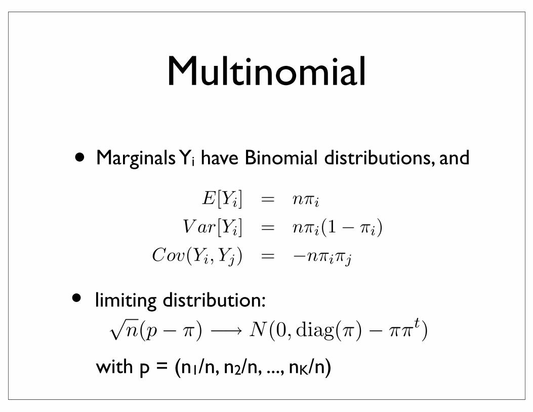
√n(p− π) −→ N(0,diag(π)− ππt)
Let Y be a (nominal) categorical variable, i.e. Y ∈ {y1, y2, ..., yK} with
P (Y = y1) = p(y1) = π1
P (Y = y2) = p(y2) = π2
K�
i=1
πi = 1
...
P (Y = yK) = p(yK) = πK
πi = P (Y = yi), 1 ≤ i ≤ K
The probability mass function then is
p(n1, n2, ..., nk) =n!
n1!n2! · ... · nk!πn1
1 πn22 · ... · πnk
k ,
3
is called a two dimensional contingency table or cross-classification table. If πij denotesthe probability of pair (xi, yj) then the table
X\Y y1 y2 ... yJ
x1 π11 π12 ... π1J π1.
x2 π21 π22 ... π2J π2....
...... . . . ...
...xI πI1 πI2 ... πIJ πI.
π.1 π.2 ... π.J 1
contains the joint distribution and {π1., π2., ...,πI.} and {π.1, π.2, ...,π.J} are marginal dis-tributions.
G2 = 2
�
i
yi log�
mi
m0,i
�= 0.74
X2 =
�
i
(mi −m0,i)2
m0,i= 0.69
Ha : 0 ≤ π ≤ 1 with π1 + π2 + π3 = 1
Ho : π = πo
πo =
0.750.18750.0625
√n(p− π) −→ N(0,diag(π)− ππt)
Let Y be a (nominal) categorical variable, i.e. Y ∈ {y1, y2, ..., yK} with
P (Y = y1) = p(y1) = π1
P (Y = y2) = p(y2) = π2
K�
i=1
πi = 1
...
P (Y = yK) = p(yK) = πK
πj = P (Yi = j), 1 ≤ j ≤ K, 1 ≤ i ≤ n
The probability mass function then is
p(n1, n2, ..., nk) =n!
n1!n2! · ... · nk!πn1
1 πn22 · ... · πnk
k ,
3
Multinomial
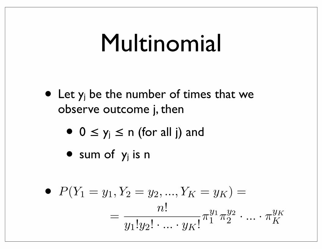
• Let yj be the number of times that we observe outcome j, then
• 0 ≤ yj ≤ n (for all j) and
• sum of yj is n
•
with n =�k
i=1 ni.
X = # of insects trapped overnight,or X = # of mosquito bites in an hour,⇒ no upper limit for n
X ∈ {0, 1, 2, 3, ...}Poisson probability mass function
P (X = x) = p(x) = e−µ µx
x!,
where λ is the rate parameter (remember, that the rate depends on the unit used).
E[X] = λ
V ar[X] = λ
skewness =√
λ
kurtosis = 1/λ
P (Y1 = y1, Y2 = y2, ..., YK = yK) =
=n!
y1!y2! · ... · yK !πy1
1 πy22 · ... · πyK
K
Yi ∼ Bn,πi E[Yi] = nπi
V ar[Yi] = nπi(1− πi)Cov(Yi, Yj) = −nπiπj
ML estimator for πi: π̂i = nin . Let L(π1, π2, ...,πk) =
�ki=1 πni
i the multinomial likelihoodfunction. With the additional constraint
�ki=1 πi = 1 the likelihood function is actually a
function in k − 1 variables:
L(π1, π2, ...,πk−1) =k−1�
i=1
πnii ·
�1−
k−1�
i=1
πi
�nk
Then
logL(π1, π2, ...,πk−1) = ni log πi + nk log
�1−
k−1�
i=1
πi
�
∂
∂πilogL(π1, π2, ...,πk−1) =
ni
πi+ nk
11−
�k−1i=1 πi
· (−1) =ni
πi− nk
πk
!= 0.
⇒ π̂i
πk=
ni
nk.
4
Multinomial
• Marginals Yi have Binomial distributions, and
• limiting distribution:
with p = (n1/n, n2/n, ..., nK/n)
with n =�k
i=1 ni.
X = # of insects trapped overnight,or X = # of mosquito bites in an hour,⇒ no upper limit for n
X ∈ {0, 1, 2, 3, ...}Poisson probability mass function
P (X = x) = p(x) = e−µ µx
x!,
where λ is the rate parameter (remember, that the rate depends on the unit used).
E[X] = λ
V ar[X] = λ
skewness =√
λ
kurtosis = 1/λ
P (Y1 = y1, Y2 = y2, ..., YK = yK) =
=n!
y1!y2! · ... · yK !πy1
1 πy22 · ... · πyK
K
Yi ∼ Bn,πi E[Yi] = nπi
V ar[Yi] = nπi(1− πi)Cov(Yi, Yj) = −nπiπj
ML estimator for πi: π̂i = nin . Let L(π1, π2, ...,πk) =
�ki=1 πni
i the multinomial likelihoodfunction. With the additional constraint
�ki=1 πi = 1 the likelihood function is actually a
function in k − 1 variables:
L(π1, π2, ...,πk−1) =k−1�
i=1
πnii ·
�1−
k−1�
i=1
πi
�nk
Then
logL(π1, π2, ...,πk−1) = ni log πi + nk log
�1−
k−1�
i=1
πi
�
∂
∂πilogL(π1, π2, ...,πk−1) =
ni
πi+ nk
11−
�k−1i=1 πi
· (−1) =ni
πi− nk
πk
!= 0.
⇒ π̂i
πk=
ni
nk.
4
is called a two dimensional contingency table or cross-classification table. If πij denotesthe probability of pair (xi, yj) then the table
X\Y y1 y2 ... yJ
x1 π11 π12 ... π1J π1.
x2 π21 π22 ... π2J π2....
...... . . . ...
...xI πI1 πI2 ... πIJ πI.
π.1 π.2 ... π.J 1
contains the joint distribution and {π1., π2., ...,πI.} and {π.1, π.2, ...,π.J} are marginal dis-tributions.
G2 = 2
�
i
yi log�
mi
m0,i
�= 0.74
X2 =
�
i
(mi −m0,i)2
m0,i= 0.69
Ha : 0 ≤ π ≤ 1 with π1 + π2 + π3 = 1
Ho : π = πo
πo =
0.750.18750.0625
√n(p− π) −→ N(0,diag(π)− ππt)
Let Y be a (nominal) categorical variable, i.e. Y ∈ {y1, y2, ..., yK} with
P (Y = y1) = p(y1) = π1
P (Y = y2) = p(y2) = π2
K�
i=1
πi = 1
...
P (Y = yK) = p(yK) = πK
πj = P (Yi = j), 1 ≤ j ≤ K, 1 ≤ i ≤ n
The probability mass function then is
p(n1, n2, ..., nk) =n!
n1!n2! · ... · nk!πn1
1 πn22 · ... · πnk
k ,
3

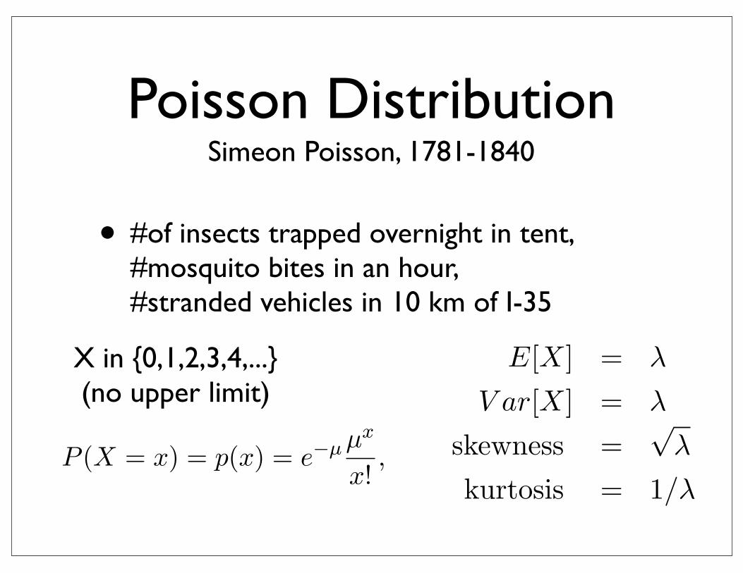
Poisson Distribution
• #of insects trapped overnight in tent, #mosquito bites in an hour, #stranded vehicles in 10 km of I-35
Simeon Poisson, 1781-1840with n =�k
i=1 ni.
X = # of insects trapped overnight,or X = # of mosquito bites in an hour,⇒ no upper limit for n
X ∈ {0, 1, 2, 3, ...}Poisson probability mass function
P (X = x) = p(x) = e−µ µx
x!,
where λ is the rate parameter (remember, that the rate depends on the unit used).
E[X] = λ
V ar[X] = λ
skewness =√
λ
kurtosis = 1/λ
P (Y1 = y1, Y2 = y2, ..., YK = yK) =
=n!
y1!y2! · ... · yK !πy1
1 πy22 · ... · πyK
K
Yi ∼ Bn,πi E[Yi] = nπi
V ar[Yi] = nπi(1− πi)Cov(Yi, Yj) = −nπiπj
ML estimator for πi: π̂i = nin . Let L(π1, π2, ...,πk) =
�ki=1 πni
i the multinomial likelihoodfunction. With the additional constraint
�ki=1 πi = 1 the likelihood function is actually a
function in k − 1 variables:
L(π1, π2, ...,πk−1) =k−1�
i=1
πnii ·
�1−
k−1�
i=1
πi
�nk
Then
logL(π1, π2, ...,πk−1) = ni log πi + nk log
�1−
k−1�
i=1
πi
�
∂
∂πilogL(π1, π2, ...,πk−1) =
ni
πi+ nk
11−
�k−1i=1 πi
· (−1) =ni
πi− nk
πk
!= 0.
⇒ π̂i
πk=
ni
nk.
4
with n =�k
i=1 ni.
X = # of insects trapped overnight,or X = # of mosquito bites in an hour,⇒ no upper limit for n
X ∈ {0, 1, 2, 3, ...}Poisson probability mass function
P (X = x) = p(x) = e−µ µx
x!,
where λ is the rate parameter (remember, that the rate depends on the unit used).
E[X] = λ
V ar[X] = λ
skewness =√
λ
kurtosis = 1/λ
P (Y1 = y1, Y2 = y2, ..., YK = yK) =
=n!
y1!y2! · ... · yK !πy1
1 πy22 · ... · πyK
K
Yi ∼ Bn,πi E[Yi] = nπi
V ar[Yi] = nπi(1− πi)Cov(Yi, Yj) = −nπiπj
ML estimator for πi: π̂i = nin . Let L(π1, π2, ...,πk) =
�ki=1 πni
i the multinomial likelihoodfunction. With the additional constraint
�ki=1 πi = 1 the likelihood function is actually a
function in k − 1 variables:
L(π1, π2, ...,πk−1) =k−1�
i=1
πnii ·
�1−
k−1�
i=1
πi
�nk
Then
logL(π1, π2, ...,πk−1) = ni log πi + nk log
�1−
k−1�
i=1
πi
�
∂
∂πilogL(π1, π2, ...,πk−1) =
ni
πi+ nk
11−
�k−1i=1 πi
· (−1) =ni
πi− nk
πk
!= 0.
⇒ π̂i
πk=
ni
nk.
4
X in {0,1,2,3,4,...} (no upper limit)
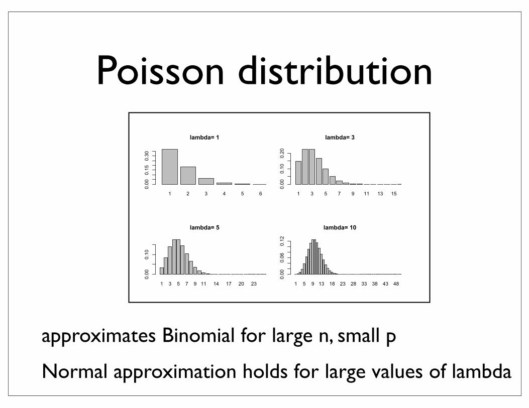
Poisson distribution
1 2 3 4 5 6
lambda= 1
0.000.150.30
1 3 5 7 9 11 13 15
lambda= 3
0.00
0.10
0.20
1 3 5 7 9 11 14 17 20 23
lambda= 5
0.00
0.10
1 5 9 13 18 23 28 33 38 43 48
lambda= 10
0.00
0.06
0.12
approximates Binomial for large n, small p
Normal approximation holds for large values of lambda
Properties of PoissonRelationship to Multinomial
• Let Y1, ..., YK be ind. Poisson with parameters µ1, ..., µK
• Y1 + ... + YK is Poisson with parameter ∑µi


Contingency Tables
• X and Y are categorical variables with I and J categories:
σ2(γ̂)∞ =16
n(ΠC + ΠD)4
I�
i=1
J�
j=1
πij
�ΠCπd
ij −ΠDπcij
�2
γ =ΠC −ΠD
ΠC + ΠD
θ :=π00 π11
π10 π01
π : (1− π)
πj|i=0 − πj|i=1 =: π1 − π2,
r :=πj=1|i=0
πj=1|i=1
χ21,0.05 = 3.84, χ2
1,0.01 = 6.634897
πij = πi+ · π+j
Ho : P ( heart disease | Cholesterol ≤ 220) =P ( heart disease | Cholesterol > 220)
π11
π11 + π12=
π21
π21 + π22
Let X, Y be two categorical variables, with I, J categories respectively and X ∈ {x1, x2, ..., xI}, Y ∈{y1, y2, ..., yJ}.
Then the pair (X, Y ) is categorical variable with IJ outcomes.The table
X\Y y1 y2 ... yJ
x1 n11 n12 ... n1J n1.
x2 n21 n22 ... n2J n2....
...... . . . ...
...xI nI1 nI2 ... nIJ nI.
n.1 n.2 ... n.J n
2
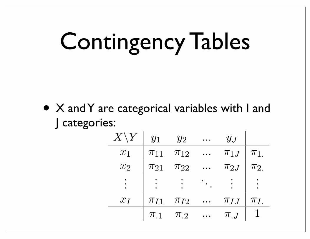
is called a two dimensional contingency table or cross-classification table. If πij denotesthe probability of pair (xi, yj) then the table
X\Y y1 y2 ... yJ
x1 π11 π12 ... π1J π1.
x2 π21 π22 ... π2J π2....
...... . . . ...
...xI πI1 πI2 ... πIJ πI.
π.1 π.2 ... π.J 1
contains the joint distribution and {π1., π2., ...,πI.} and {π.1, π.2, ...,π.J} are marginal dis-tributions.
G2 = 2
�
i
yi log�
mi
m0,i
�= 0.74
X2 =
�
i
(mi −m0,i)2
m0,i= 0.69
Ha : 0 ≤ π ≤ 1 with π1 + π2 + π3 = 1
Ho : π = πo
πo =
0.750.18750.0625
√n(p− π) −→ N(0,diag(π)− ππt)
Let Y be a (nominal) categorical variable, i.e. Y ∈ {y1, y2, ..., yK} with
P (Y = y1) = p(y1) = π1
P (Y = y2) = p(y2) = π2
K�
i=1
πi = 1
...
P (Y = yK) = p(yK) = πK
πj = P (Yi = j), 1 ≤ j ≤ K, 1 ≤ i ≤ n
The probability mass function then is
p(n1, n2, ..., nk) =n!
n1!n2! · ... · nk!πn1
1 πn22 · ... · πnk
k ,
3
Contingency Tables
• X and Y are categorical variables with I and J categories:
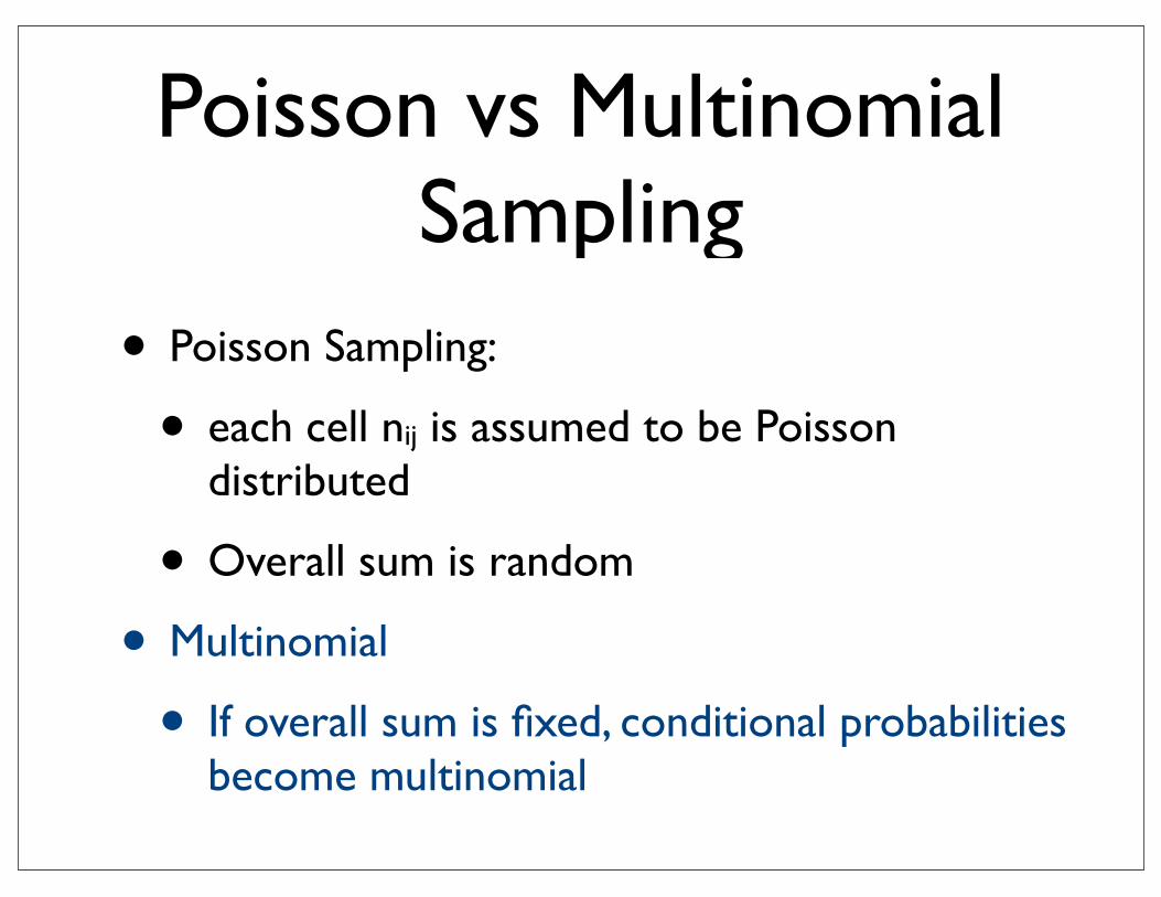
Poisson vs Multinomial Sampling
• Poisson Sampling:
• each cell nij is assumed to be Poisson distributed
• Overall sum is random
• Multinomial
• If overall sum is fixed, conditional probabilities become multinomial
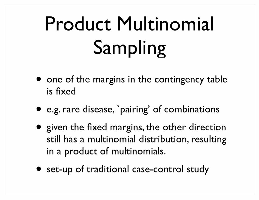
Product Multinomial Sampling
• one of the margins in the contingency table is fixed
• e.g. rare disease, `pairing’ of combinations
• given the fixed margins, the other direction still has a multinomial distribution, resulting in a product of multinomials.
• set-up of traditional case-control study
Margins are fixed
• Both margins are fixed
• less frequent in studies, more frequent in inferential methods
• Hypergeometric distribution
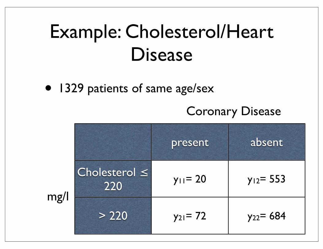
Example: Cholesterol/Heart Disease
• 1329 patients of same age/sex
present absent
Cholesterol ≤ 220
> 220
y11= 20 y12= 553
y21= 72 y22= 684
mg/l
Coronary Disease
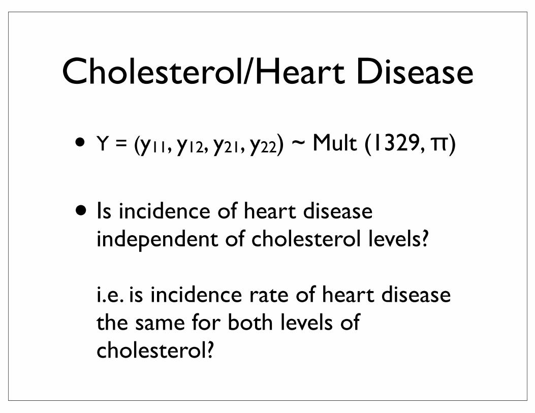
Cholesterol/Heart Disease
• Y = (y11, y12, y21, y22) ~ Mult (1329, π)
• Is incidence of heart disease independent of cholesterol levels?
i.e. is incidence rate of heart disease the same for both levels of cholesterol?
σ2(γ̂)∞ =16
n(ΠC + ΠD)4
I�
i=1
J�
j=1
πij
�ΠCπd
ij −ΠDπcij
�2
γ =ΠC −ΠD
ΠC + ΠD
θ :=π00 π11
π10 π01
π : (1− π)
πj|i=0 − πj|i=1 =: π1 − π2,
r :=πj=1|i=0
πj=1|i=1
χ21,0.05 = 3.84, χ2
1,0.01 = 6.634897
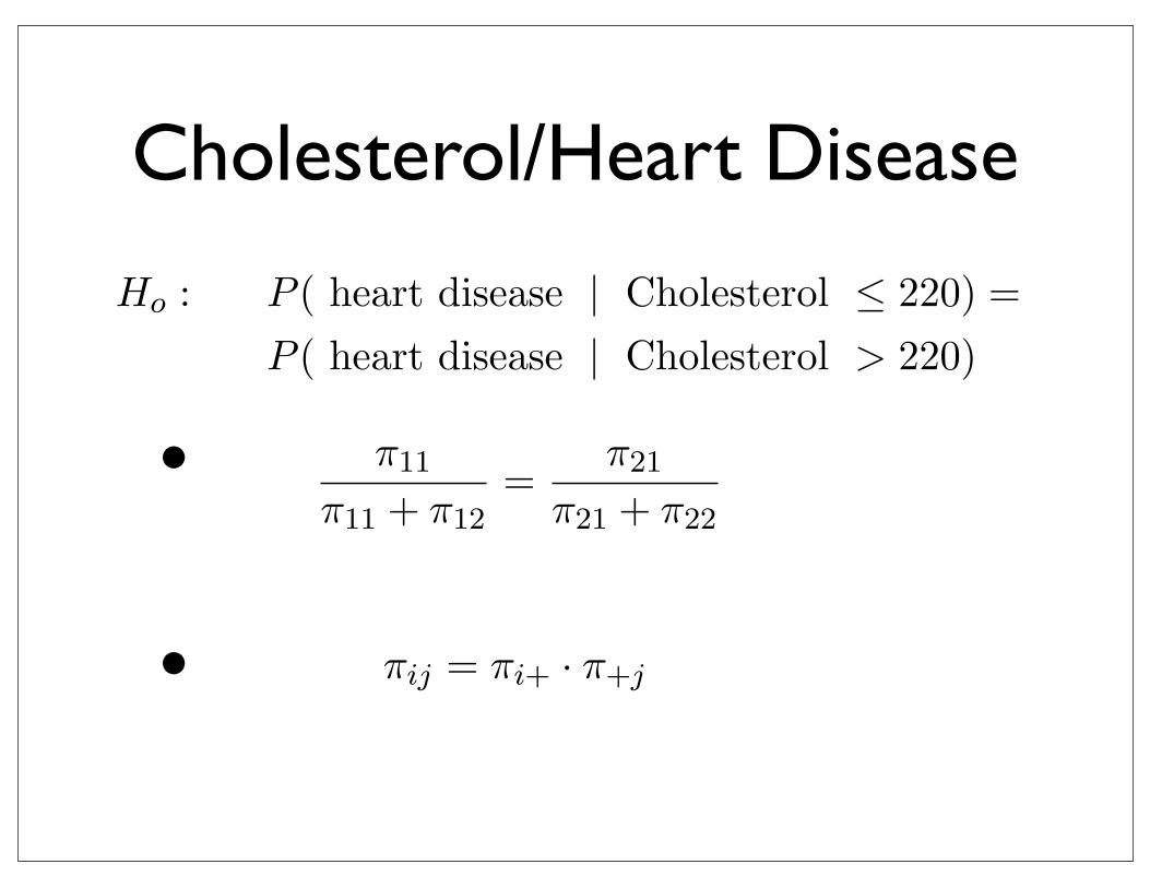
πij = πi+ · π+j
Ho : P ( heart disease | Cholesterol ≤ 220) =P ( heart disease | Cholesterol > 220)
π11
π11 + π12=
π21
π21 + π22
Let X, Y be two categorical variables, with I, J categories respectively and X ∈ {x1, x2, ..., xI}, Y ∈{y1, y2, ..., yJ}.
Then the pair (X, Y ) is categorical variable with IJ outcomes.The table
X\Y y1 y2 ... yJ
x1 n11 n12 ... n1J n1.
x2 n21 n22 ... n2J n2....
...... . . . ...
...xI nI1 nI2 ... nIJ nI.
n.1 n.2 ... n.J n
2
Cholesterol/Heart Disease
• equivalent to
• equivalent to
σ2(γ̂)∞ =16
n(ΠC + ΠD)4
I�
i=1
J�
j=1
πij
�ΠCπd
ij −ΠDπcij
�2
γ =ΠC −ΠD
ΠC + ΠD
θ :=π00 π11
π10 π01
π : (1− π)
πj|i=0 − πj|i=1 =: π1 − π2,
r :=πj=1|i=0
πj=1|i=1
χ21,0.05 = 3.84, χ2
1,0.01 = 6.634897
πij = πi+ · π+j
Ho : P ( heart disease | Cholesterol ≤ 220) =P ( heart disease | Cholesterol > 220)
π11
π11 + π12=
π21
π21 + π22
Let X, Y be two categorical variables, with I, J categories respectively and X ∈ {x1, x2, ..., xI}, Y ∈{y1, y2, ..., yJ}.
Then the pair (X, Y ) is categorical variable with IJ outcomes.The table
X\Y y1 y2 ... yJ
x1 n11 n12 ... n1J n1.
x2 n21 n22 ... n2J n2....
...... . . . ...
...xI nI1 nI2 ... nIJ nI.
n.1 n.2 ... n.J n
2
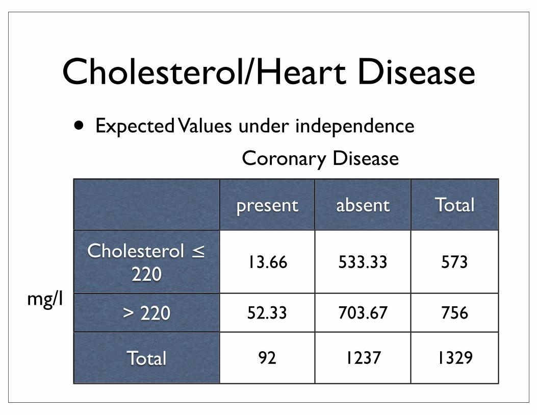
Cholesterol/Heart Disease• Expected Values under independence
present absent Total
Cholesterol ≤ 220
> 220
Total
13.66 533.33 573
52.33 703.67 756
92 1237 1329
mg/l
Coronary Disease
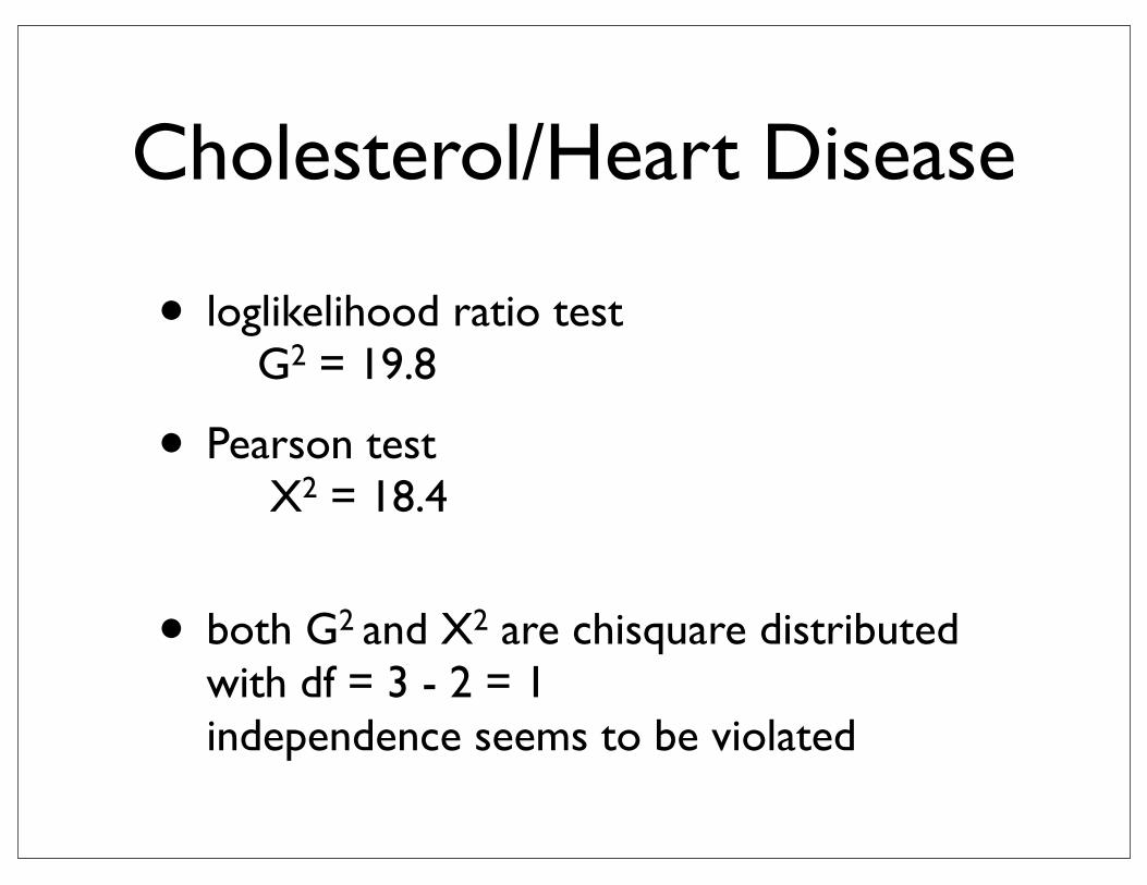
Cholesterol/Heart Disease
• loglikelihood ratio test G2 = 19.8
• Pearson test X2 = 18.4
• both G2 and X2 are chisquare distributed with df = 3 - 2 = 1independence seems to be violated

Visualizing Contingency Tables

• Area plots (i.e. area represents #combinations)
• Built hierarchically, i.e. order of variables matters
• in R:mosaicplot() (base package)imosaic() (iplots package)productplots package
http://cran.r-project.org/doc/contrib/Short-refcard.pdf
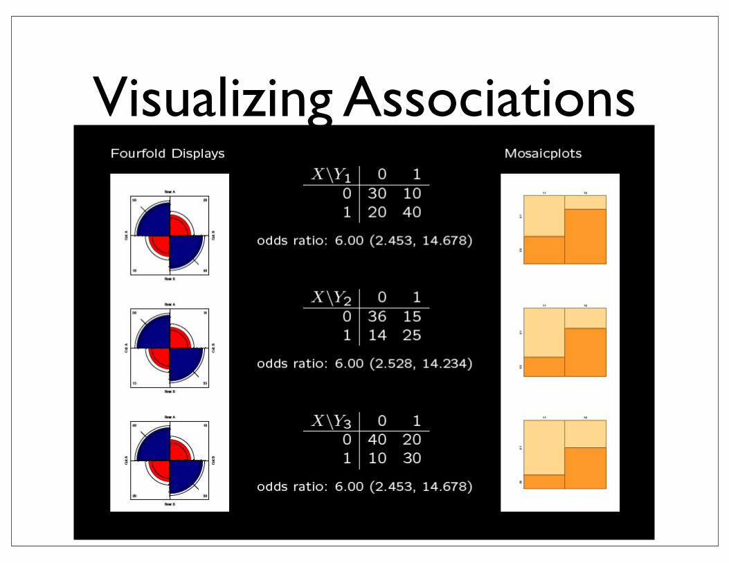
Mosaicplots
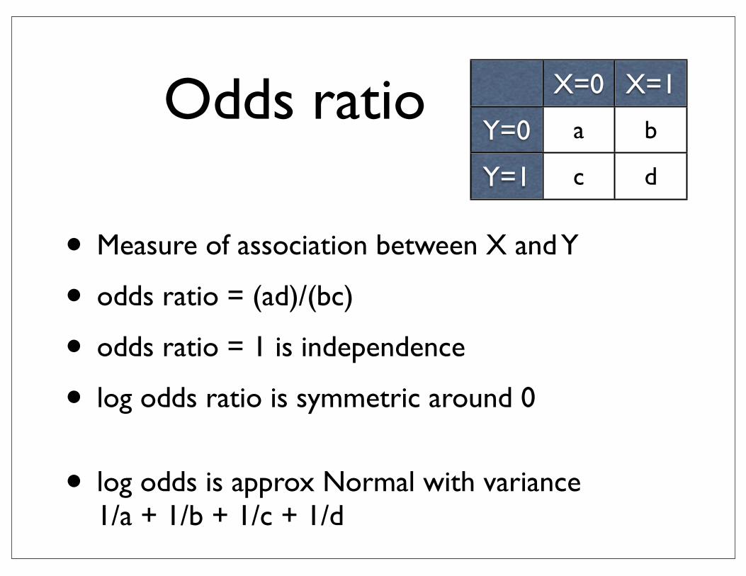
• Measure of association between X and Y
• odds ratio = (ad)/(bc)
• odds ratio = 1 is independence
• log odds ratio is symmetric around 0
• log odds is approx Normal with variance 1/a + 1/b + 1/c + 1/d
X=0 X=1
Y=0
Y=1
a b
c d
Odds ratio
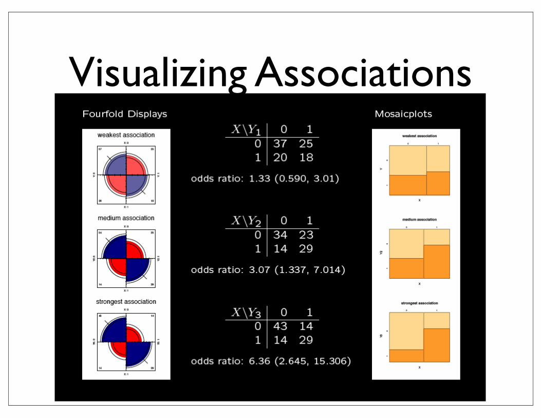
Visualizing Associations
Visualizing Associations
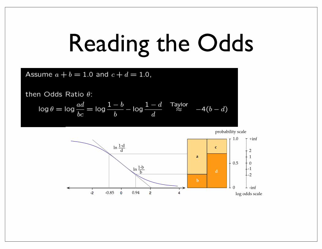
Reading the Odds
0.94
1-bbln
1-ddln
-0.85
+inf
0
-inf
2
-2-1
1
log odds scale
0.5
probability scale
0
1.0
b
a
d
c
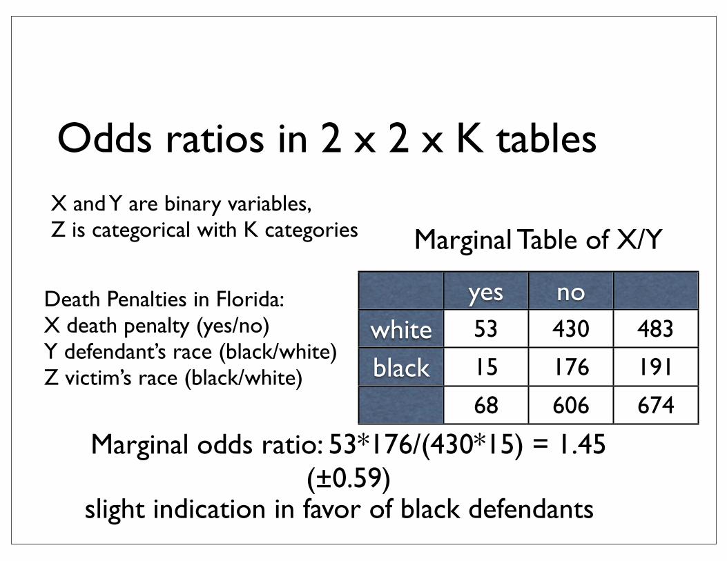
X and Y are binary variables, Z is categorical with K categories
Death Penalties in Florida:X death penalty (yes/no)Y defendant’s race (black/white)Z victim’s race (black/white)
yes nowhiteblack
53 430 483
15 176 191
68 606 674
Marginal Table of X/Y
Marginal odds ratio: 53*176/(430*15) = 1.45 (±0.59)
slight indication in favor of black defendants
Odds ratios in 2 x 2 x K tables
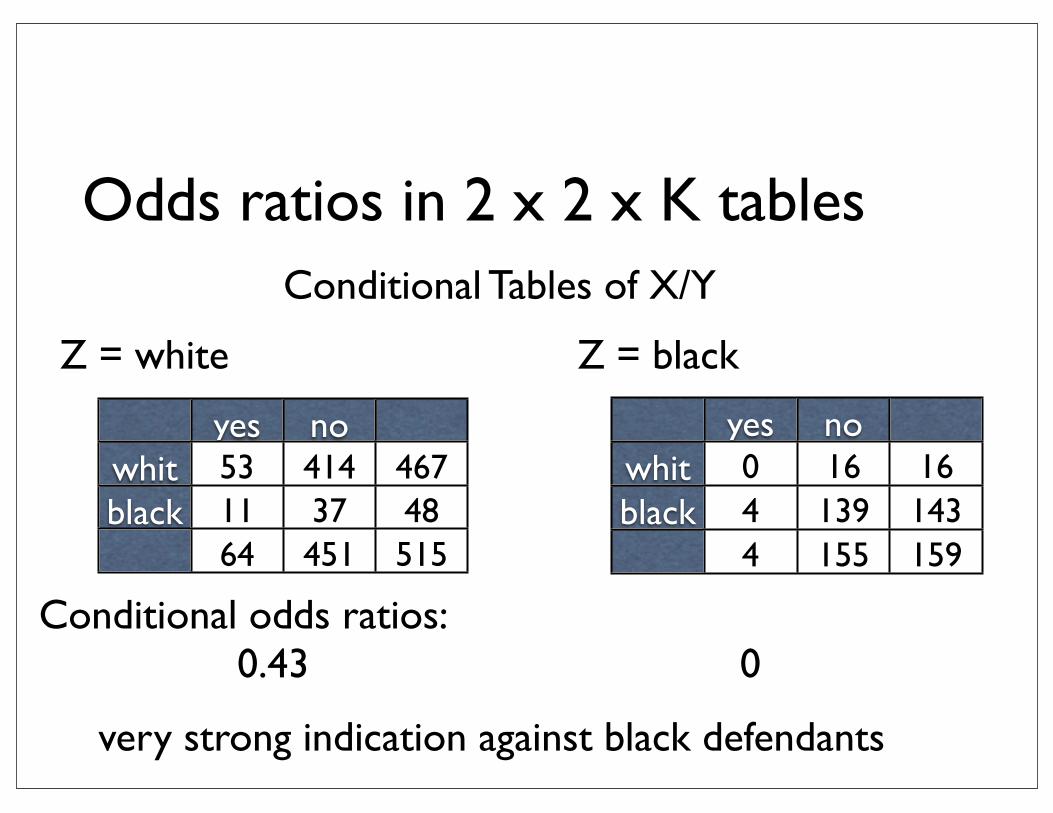
yes nowhiteblack
53 414 46711 37 4864 451 515
Conditional Tables of X/Y
Conditional odds ratios:0.43 0
Z = white
yes nowhiteblack
0 16 164 139 1434 155 159
Z = black
very strong indication against black defendants
Odds ratios in 2 x 2 x K tables
• Simpson’s paradox: marginal association between X and Y is opposite to conditional associations between X and Y for each level of Z
• due to: very strong association between X and Z or Y and Z
Simpson’s paradox
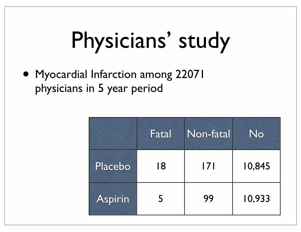
Physicians’ study• Myocardial Infarction among 22071
physicians in 5 year period
Fatal Non-fatal No
Placebo
Aspirin
18 171 10,845
5 99 10,933