Bayes - Summer 2017 - Kirchkamp · Contents 5 © Oliver Kirchkamp 1 Introduction 1.1 Preliminaries...

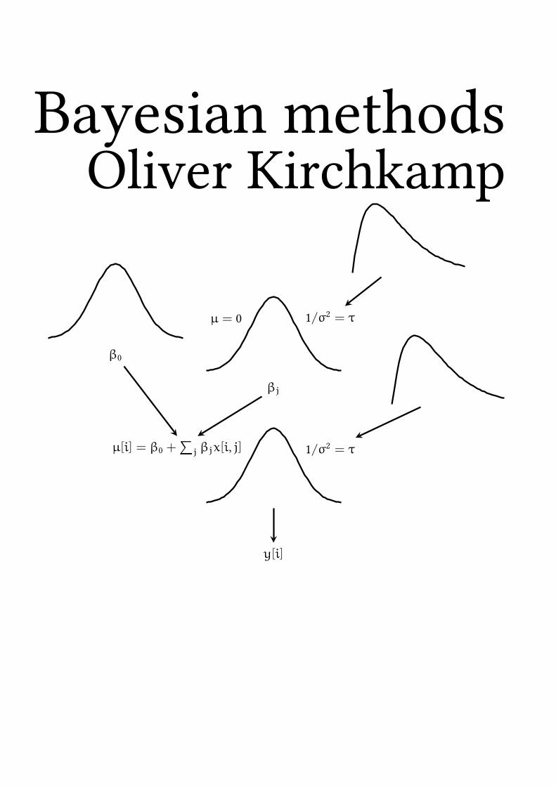
Bayesian methodsOliver Kirchkamp

βj

µ = 0 1/σ2 = τ

β0

y[i]

µ[i] = β0 +∑

j βjx[i, j] 1/σ2 = τ

2©Oliver

Kirchkam

p

13 August 2017 16:50:26

Contents

1 Introduction 5

1.1 Preliminaries . . . . . . . . . . . . . . . . . . . . . . . . . . . . . . . . . . 51.2 Motivation . . . . . . . . . . . . . . . . . . . . . . . . . . . . . . . . . . . 51.3 Using Bayesian inference . . . . . . . . . . . . . . . . . . . . . . . . . . . 51.4 The intention of the researcher — p-hacking . . . . . . . . . . . . . . . . 91.5 Compare: The Maximum Likelihood estimator . . . . . . . . . . . . . . . 111.6 Terminology . . . . . . . . . . . . . . . . . . . . . . . . . . . . . . . . . . 14

1.6.1 Probabilities . . . . . . . . . . . . . . . . . . . . . . . . . . . . . . 141.6.2 Prior information . . . . . . . . . . . . . . . . . . . . . . . . . . . 151.6.3 Objectivity and subjectivity . . . . . . . . . . . . . . . . . . . . . 151.6.4 Issues . . . . . . . . . . . . . . . . . . . . . . . . . . . . . . . . . 16

1.7 Decision making . . . . . . . . . . . . . . . . . . . . . . . . . . . . . . . . 161.8 Technical Background . . . . . . . . . . . . . . . . . . . . . . . . . . . . . 18

2 A practical example 19

2.1 The distribution of the population mean . . . . . . . . . . . . . . . . . . 192.2 Gibbs sampling . . . . . . . . . . . . . . . . . . . . . . . . . . . . . . . . 222.3 Convergence . . . . . . . . . . . . . . . . . . . . . . . . . . . . . . . . . . 232.4 Distribution of the posterior . . . . . . . . . . . . . . . . . . . . . . . . . 252.5 Accumulating evidence . . . . . . . . . . . . . . . . . . . . . . . . . . . . 252.6 Priors . . . . . . . . . . . . . . . . . . . . . . . . . . . . . . . . . . . . . . 26

3 Conjugate Priors 26

3.1 Accumulating evidence, continued . . . . . . . . . . . . . . . . . . . . . . 263.2 Normal Likelihood . . . . . . . . . . . . . . . . . . . . . . . . . . . . . . . 273.3 Bernoulli Likelihood . . . . . . . . . . . . . . . . . . . . . . . . . . . . . . 293.4 Problems with the analytical approach . . . . . . . . . . . . . . . . . . . 293.5 Exercises . . . . . . . . . . . . . . . . . . . . . . . . . . . . . . . . . . . . 30

4 Linear Regression 30

4.1 Introduction . . . . . . . . . . . . . . . . . . . . . . . . . . . . . . . . . . 304.2 Demeaning . . . . . . . . . . . . . . . . . . . . . . . . . . . . . . . . . . . 334.3 Correlation . . . . . . . . . . . . . . . . . . . . . . . . . . . . . . . . . . . 374.4 The three steps of the Gibbs sampler . . . . . . . . . . . . . . . . . . . . 394.5 Exercises . . . . . . . . . . . . . . . . . . . . . . . . . . . . . . . . . . . . 40

5 Finding posteriors 40

5.1 Overview . . . . . . . . . . . . . . . . . . . . . . . . . . . . . . . . . . . . 405.2 Example for the exact way: . . . . . . . . . . . . . . . . . . . . . . . . . . 405.3 Rejection sampling . . . . . . . . . . . . . . . . . . . . . . . . . . . . . . 415.4 Metropolis-Hastings . . . . . . . . . . . . . . . . . . . . . . . . . . . . . . 42

Contents 3

©Oliver

Kirchkam

p

5.5 Gibbs sampling . . . . . . . . . . . . . . . . . . . . . . . . . . . . . . . . 435.6 Check convergence . . . . . . . . . . . . . . . . . . . . . . . . . . . . . . 46

5.6.1 Gelman, Rubin (1992): potential scale reduction factor . . . . . . 465.7 A better vague prior for τ . . . . . . . . . . . . . . . . . . . . . . . . . . . 515.8 More on History . . . . . . . . . . . . . . . . . . . . . . . . . . . . . . . . 53

6 Robust regression 54

6.1 Robust regression with the Crime data . . . . . . . . . . . . . . . . . . . 546.2 Robust regression with the Engel data . . . . . . . . . . . . . . . . . . . . 596.3 Exercises . . . . . . . . . . . . . . . . . . . . . . . . . . . . . . . . . . . . 61

7 Nonparametric 62

7.1 Preliminaries . . . . . . . . . . . . . . . . . . . . . . . . . . . . . . . . . . 627.2 Example: Rank sum based comparison . . . . . . . . . . . . . . . . . . . 62

8 Identification 66

9 Discrete Choice 70

9.1 Labor force participation . . . . . . . . . . . . . . . . . . . . . . . . . . . 709.2 A generalised linear model . . . . . . . . . . . . . . . . . . . . . . . . . . 709.3 Bayesian discrete choice . . . . . . . . . . . . . . . . . . . . . . . . . . . 719.4 Exercise . . . . . . . . . . . . . . . . . . . . . . . . . . . . . . . . . . . . . 72

10 Count data 72

10.1 Poisson model . . . . . . . . . . . . . . . . . . . . . . . . . . . . . . . . . 7210.2 Negative binomial . . . . . . . . . . . . . . . . . . . . . . . . . . . . . . . 7410.3 Exercise . . . . . . . . . . . . . . . . . . . . . . . . . . . . . . . . . . . . . 76

11 Multinomial (polytomous) logit 76

11.1 Motivation and background . . . . . . . . . . . . . . . . . . . . . . . . . 7611.2 Example . . . . . . . . . . . . . . . . . . . . . . . . . . . . . . . . . . . . 8011.3 Bayesian multinomial . . . . . . . . . . . . . . . . . . . . . . . . . . . . . 8311.4 Exercise . . . . . . . . . . . . . . . . . . . . . . . . . . . . . . . . . . . . . 84

12 Ordered probit 84

12.1 Model . . . . . . . . . . . . . . . . . . . . . . . . . . . . . . . . . . . . . . 8412.2 Illustration — the Fair data . . . . . . . . . . . . . . . . . . . . . . . . . . 8612.3 Exercise . . . . . . . . . . . . . . . . . . . . . . . . . . . . . . . . . . . . . 91

13 Instrumental variables 91

13.1 Example: Demand and Supply . . . . . . . . . . . . . . . . . . . . . . . . 9313.2 Discrete endogeneous variables . . . . . . . . . . . . . . . . . . . . . . . 9813.3 Exercises . . . . . . . . . . . . . . . . . . . . . . . . . . . . . . . . . . . . 101

4©Oliver

Kirchkam

p

13 August 2017 16:50:26

14 Measurement errors 101

14.1 Single measures, known error . . . . . . . . . . . . . . . . . . . . . . . . 101

14.2 Multiple measures . . . . . . . . . . . . . . . . . . . . . . . . . . . . . . . 105

14.3 Aggregating evidence . . . . . . . . . . . . . . . . . . . . . . . . . . . . . 106

15 Selection 112

15.1 Interval regression . . . . . . . . . . . . . . . . . . . . . . . . . . . . . . . 112

15.2 Bayesian censored model . . . . . . . . . . . . . . . . . . . . . . . . . . . 114

15.3 Heckman correction . . . . . . . . . . . . . . . . . . . . . . . . . . . . . . 116

15.4 Bayesian Heckman correction . . . . . . . . . . . . . . . . . . . . . . . . 119

15.5 Exercise . . . . . . . . . . . . . . . . . . . . . . . . . . . . . . . . . . . . . 120

16 More on initialisation 120

17 Hierarchical Models 121

17.1 Mixed effects . . . . . . . . . . . . . . . . . . . . . . . . . . . . . . . . . . 121

17.2 Example: Crime in North Carolina . . . . . . . . . . . . . . . . . . . . . . 121

17.3 Bayes and mixed effects . . . . . . . . . . . . . . . . . . . . . . . . . . . . 123

17.4 Robust mixed effects . . . . . . . . . . . . . . . . . . . . . . . . . . . . . 124

17.5 Exercises . . . . . . . . . . . . . . . . . . . . . . . . . . . . . . . . . . . . 127

18 Model Comparison 127

18.1 Example 1 . . . . . . . . . . . . . . . . . . . . . . . . . . . . . . . . . . . 128

18.2 Example 2 . . . . . . . . . . . . . . . . . . . . . . . . . . . . . . . . . . . 129

18.3 Model 1 . . . . . . . . . . . . . . . . . . . . . . . . . . . . . . . . . . . . . 131

18.4 Model 2 . . . . . . . . . . . . . . . . . . . . . . . . . . . . . . . . . . . . . 131

18.5 A joint model . . . . . . . . . . . . . . . . . . . . . . . . . . . . . . . . . 132

18.6 Pseudopriors . . . . . . . . . . . . . . . . . . . . . . . . . . . . . . . . . . 136

18.7 Model uncertainty . . . . . . . . . . . . . . . . . . . . . . . . . . . . . . . 139

18.8 Bayes factors . . . . . . . . . . . . . . . . . . . . . . . . . . . . . . . . . . 140

19 Mixture Models 140

19.1 Example . . . . . . . . . . . . . . . . . . . . . . . . . . . . . . . . . . . . 140

19.2 Labels and sorting . . . . . . . . . . . . . . . . . . . . . . . . . . . . . . . 142

19.3 More groups . . . . . . . . . . . . . . . . . . . . . . . . . . . . . . . . . . 143

19.4 Ordering, not sorting . . . . . . . . . . . . . . . . . . . . . . . . . . . . . 145

19.5 Using dnormmix . . . . . . . . . . . . . . . . . . . . . . . . . . . . . . . . 146

19.6 Exercises . . . . . . . . . . . . . . . . . . . . . . . . . . . . . . . . . . . . 147

20 Summary 147

21 Exercises 148

Contents 5

©Oliver

Kirchkam

p

1 Introduction

1.1 Preliminaries

Purpose of this handout In this handout you find the content of the slides I am usingin the lecture. The handout is not supposed to replace a book. I recommend some bookson the webpage and in the course.

Homepage: hp://www.kirchkamp.de/

Literature:

• Kruschke, Doing Bayesian Data Analysis

• Hoff, A First Course in Bayesian Statistical Methods.

To learn more about MCMC sampling you can also read C. Andrieu, de Freitas, N.,Doucet, A, Jordan, M. “An Introduction toMCMC forMachine Learning.” Machine Learn-ing. 2003, 50(1-2), pp 5-43.

Aim of the course

• Compare Bayesian with frequentist methods.

Two schools of statistical inference: Bayesian / Frequentist

– Frequentist: Standard hypothesis testing, p-values, confidence intervals. Wellknown.

– Bayesian: beliefs conditional on data.

• Learn to apply Bayesian methods.

– What is the equivalent of frequentist method X in the Bayesian world?

– How to put Bayesian methods into practice?

1.2 Motivation

1.3 Using Bayesian inference

Pros:

• Prior knowledge

• Model identification is less strict

• Small-sample size

• Non-standard models

http://www.kirchkamp.de/

6©Oliver

Kirchkam

p

13 August 2017 16:50:26

– Non-normal distributions

– Categorical data

– Multi-level models

– Missing values

– Latent variables

• Interpretation

Cons:

• Prior knowledge

• Computationally expensive

• Model-fit diagnostic

Comparison Frequentist: NullHypothesis SignificanceTesting (RonaldA. Fisher,Statistical Methods for Research Workers, 1925, p. 43)

• X← θ, X is random, θ is fixed.

• Confidence intervals and p-values are easy to calculate.

• Interpretation of confidence intervals and p-values is awkward.

• p-values depend on the intention of the researcher.

• We can test “Null-hypotheses” (but where do these Null-hypotheses come from).

• Not good at accumulating knowledge.

• More restrictive modelling.

Bayesian: (Thomas Bayes, 1702-1761; Metropolis et al., “Equations of State Cal-culations by Fast Computing Machines”. Journal of Chemical Physics, 1953.)

• X→ θ, X is fixed, θ is random.

• Requires more computational effort.

• “Credible intervals” are easier to interpret.

• Can work with “uninformed priors” (similar results as with frequentist statistics)

Contents 7

©Oliver

Kirchkam

p

• Efficient at accumulating knowledge.

• Flexible modelling.

Most people are still used to the frequentist approach. Although the Bayesian approachmight have clear advantages it is important that we are able to understand research thatis done in the context of the frequentist approach.

Pr(A∧ B) = Pr(A) · Pr(B|A) = Pr(B) · Pr(A|B)

rewrite: Pr(A) · Pr(B|A) 1

Pr(B)= Pr(A|B)

with A = θ︸︷︷︸parameter

and B = X︸︷︷︸data

:

Pr(θ)︸︷︷︸prior

· Pr(X|θ)︸︷︷︸likelihood

· 1

Pr(X)︸︷︷︸

∫Pr(θ) Pr(X|θ)dθ

= Pr(θ|X)︸︷︷︸posterior

Before we come to a more formal comparison, let us compare the two approaches,frequentist versus Bayesian, with the help of an example.I will use an example from the legal profession. Courts have to decide whether a

defendant is guilty or innocent. Scientists have to decide whether a hypothesis is corrector not correct. Statistically, in both cases we are talking about the value of a parameter.θ = guilty or θ = not guilty. Alternatively, β = 0 or β 6= 0.My hope is that the legal context makes it more obvious how the decision process fails

or succeeds.

The prosecutors’ fallacyAssuming that the prior probability of a random match is equal to the probability thatthe defendant is innocent.

Two problems:

• p-values depend on the researcher’s intention. E.g. multiple testing (several sus-pects, perhaps the entire population, is “tested”, only one suspect is brought totrial)

• Conditional probability (neglecting prior probabilities of the crime)

• Lucia de Berk:

– Pr(evidence|not guilty) = 1/342 million

– Pr(evidence|not guilty) = 1/25

8©Oliver

Kirchkam

p

13 August 2017 16:50:26

• Sally Clark

– Pr(evidence|not guilty) = 1/73 million

– Pr(not guilty|evidence) = 78%

The Sally Clark case

• 1996: First child dies from SIDS (sudden infant death syndrome): P = 1/8543

• 1998: Second child dies from SIDS: P = 1/8543

• →: Pr(evidence|not guilty) = (1/8543)2 ≈ 1/73 million

• 1999: life imprisonment, upheld at appeal in 2000.

Problems:

• Correlation of SIDS within a family. Pr(2nd child) = (1/8543)× 5 . . . 10

• SIDS is actually more likely in this case: P = 1/8543→ P = 1/1300

Pr(evidence|1 not guilty mother) = 1/(1300 · 130) = 0.000592 %

• Intention of the researcher/multiple testing: ≈ 750 000 births in England andWales/ year. How likely is it to find two successive SIDS or more among 750 000 mothers.

Pr(evidence|750 000 not guilty mothers) = 98.8 %.

But what is the (posterior) probability of guilt? Here we need prior information.

• What is the prior probability of a mother murdering her child?



· 1

Pr(X)= Pr(θ|X)

︸︷︷︸posterior

Pr(g)︸︷︷︸prior

· Pr(X|g)︸︷︷︸likelihood

· 1

Pr(g) · Pr(X|g) + (1− Pr(g)) · Pr(X|not g)︸︷︷︸

Pr(X)

= Pr(g|X)︸︷︷︸posterior

Data from the U.S.A. (Miller, Oberman, 2004): per 600 000 mothers 1 killed child,Pr(g) = 1/600 000.

Pr(X|g) = 1, Pr(X) = 1600 000︸︷︷︸guilty

+ 599 999600 000

· 11300·130︸︷︷︸

not guilty

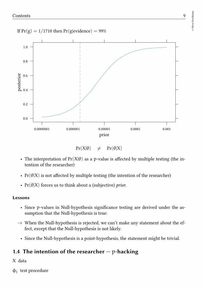
Pr(g|evidence) = 22%

If Pr(g) = 1/18800 then Pr(g|evidence) = 90%

Contents 9

©Oliver

Kirchkam

p

If Pr(g) = 1/1710 then Pr(g|evidence) = 99%

prior

posterior

0.0

0.2

0.4

0.6

0.8

1.0

0.0000001 0.000001 0.00001 0.0001 0.001

Pr(X|θ) 6= Pr(θ|X)

• The interpretation of Pr(X|θ) as a p-value is affected by multiple testing (the in-tention of the researcher)

• Pr(θ|X) is not affected by multiple testing (the intention of the researcher)

• Pr(θ|X) forces us to think about a (subjective) prior.

Lessons

• Since p-values in Null-hypothesis significance testing are derived under the as-sumption that the Null-hypothesis is true:

→ When the Null-hypothesis is rejected, we can’t make any statement about the ef-fect, except that the Null-hypothesis is not likely.

• Since the Null-hypothesis is a point-hypothesis, the statement might be trivial.

1.4 The intention of the researcher — p-hacking

X data

φj test procedure

10©Oliver

Kirchkam

p

13 August 2017 16:50:26

• choice of control variables

• data exclusion

• coding

• analysis

• interactions

• predictors

•...

T(X,φj) test result

p-hacking

• perform J tests: . . . , T(X,φj), . . .

• report the best result, given the data: T(X,φbest)

→ to correct for multiple testing we need to know J ↓

→ robustness checks (for all J ↓)

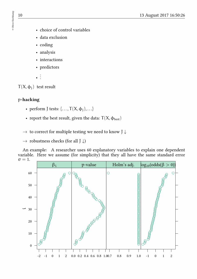
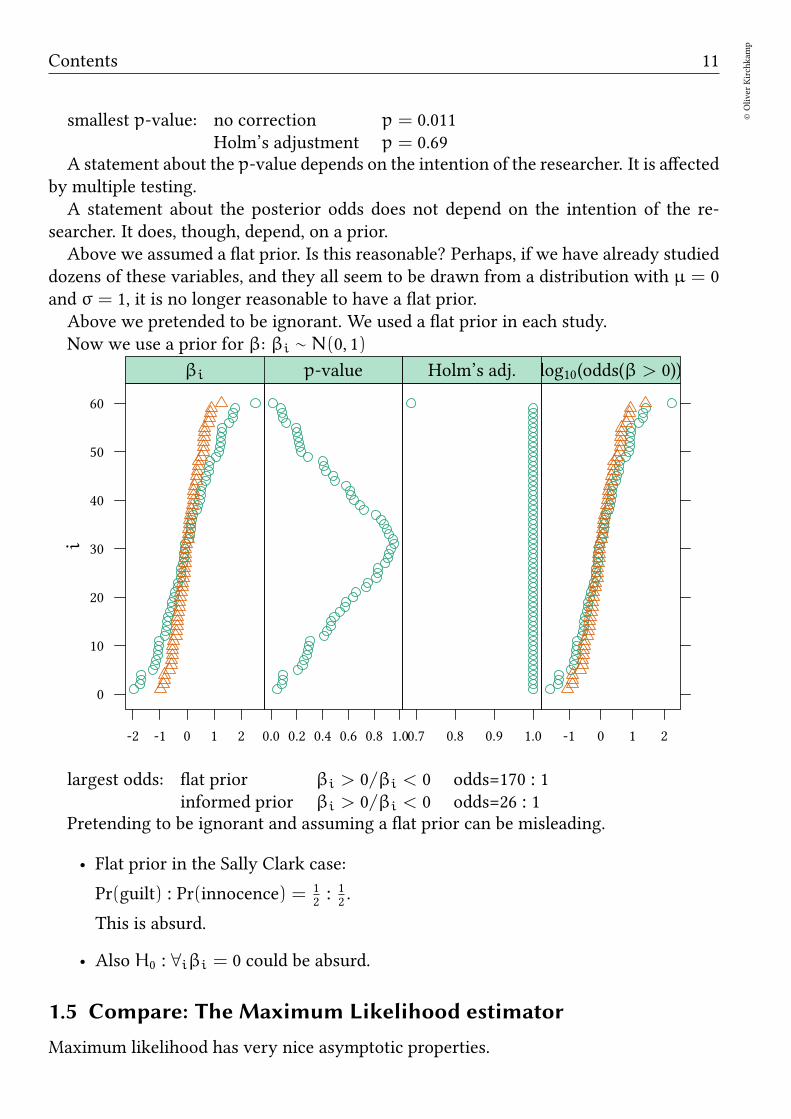
An example: A researcher uses 60 explanatory variables to explain one dependentvariable. Here we assume (for simplicity) that they all have the same standard errorσ = 1.

i

0

10

20

30

40

50

60

-2 -1 0 1 2

βi

0.0 0.2 0.4 0.6 0.8 1.0

p-value

0.7 0.8 0.9 1.0

Holm’s adj.

-1 0 1 2

log10(odds(β > 0))

Contents 11

©Oliver

Kirchkam

p

smallest p-value: no correction p = 0.011Holm’s adjustment p = 0.69

A statement about the p-value depends on the intention of the researcher. It is affectedby multiple testing.A statement about the posterior odds does not depend on the intention of the re-

searcher. It does, though, depend, on a prior.Above we assumed a flat prior. Is this reasonable? Perhaps, if we have already studied

dozens of these variables, and they all seem to be drawn from a distribution with µ = 0and σ = 1, it is no longer reasonable to have a flat prior.Above we pretended to be ignorant. We used a flat prior in each study.Now we use a prior for β: βi ∼ N(0, 1)

i

0

10

20

30

40

50

60

-2 -1 0 1 2

βi

0.0 0.2 0.4 0.6 0.8 1.0

p-value

0.7 0.8 0.9 1.0

Holm’s adj.

-1 0 1 2

log10(odds(β > 0))

largest odds: flat prior βi > 0/βi < 0 odds=170 : 1informed prior βi > 0/βi < 0 odds=26 : 1

Pretending to be ignorant and assuming a flat prior can be misleading.

• Flat prior in the Sally Clark case:

Pr(guilt) : Pr(innocence) = 12: 12.

This is absurd.

• Also H0 : ∀iβi = 0 could be absurd.

1.5 Compare: The Maximum Likelihood estimator

Maximum likelihood has very nice asymptotic properties.

12©Oliver

Kirchkam

p

13 August 2017 16:50:26

But what if the assumptions for these properties are not fulfilled?

• Consistency

• Asymptotic normality

– θ0 must be away from the boundary (not trivial with panel data).

– the number of nuisance parameters must not increase with the sample size(not trivial with panel data).

–...

• Efficiency when the sample size tends to infinity

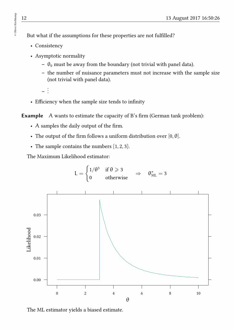
Example A wants to estimate the capacity of B’s firm (German tank problem):

• A samples the daily output of the firm.

• The output of the firm follows a uniform distribution over [0, θ].

• The sample contains the numbers 1, 2, 3.

The Maximum Likelihood estimator:

L =

1/θ3 if θ > 3

0 otherwise⇒ θ∗ML = 3

θ

Likelihood

0.00

0.01

0.02

0.03

0 2 4 6 8 10

The ML estimator yields a biased estimate.

Contents 13

©Oliver

Kirchkam

p

For a Bayesian estimate we need a prior. Let us assume that A assumes all capacitiesbetween 0 andM to be equally likely. Then (for θ > 3):

Pr(θ|X) =Pr(θ) · Pr(X|θ)

∫Pr(θ) Pr(X|θ)dθ

=1M

1θ3

∫M3

1M

1θ3 dθ

=18M2

(M2 − 9)θ3

Hence

E(θ) =

∫

θ · f(θ)dθ =

∫M

3

θ · Pr(θ|x)dθ =6M

M+ 3

E.g. ifM = 10, then E(θ) = 60/13 = 4.615. IfM = 100, then E(θ) = 600/103 = 5.825.

θ

Pr(θ|X)

0.0

0.2

0.4

0.6

0 2 4 6 8 10

E(m)Q2.5% Q97.5%

Remember: density function:

Pr(θ|X) =18M2

(M2 − 9)θ3

Distribution function:

F(q) =

∫q

3

Pr(θ|x)dθ =M2(q2 − 9)

(M2 − 9)q2

Quantile function:

Solve F(q) = p ⇒ Q(p) =3M

√

(1− p)M2 + 9p

ForM = 10 we have CI[2.5%,97.5%] =[

20·√30√

1303, 6·10

3/2√451

]

= [3.035, 8.743]

14©Oliver

Kirchkam

p

13 August 2017 16:50:26

1.6 Terminology

1.6.1 Probabilities

Consider the following statements:

Frequentist probability

• The probability to throw two times a six is 1/36.

• The probability to win the state lottery is about 1:175 000 000.

• The probability of rainfall on a given day in August is 1/3.

• The probability for a male human to develop lung or bronchus cancer is 7.43%.

Subjective probability

• The probability of rainfall tomorrow is 1/3.

• The probability that a Mr. Smith develops lung or bronchus cancer is 7.43%.

• The probability that Ms. X commited a crime is 20%.

Frequentist

• P = objective probability (sampling of the data X is infinite).

→ but what if the event occurs only once (rainfall tomorrow, Mr. Smith’s health,. . . )?

→ von Mises: event has no probability

→ Popper: invent a fictitious population from which the even is a random sam-ple (propensity probability).

• Parameters θ are unknown but fixed during repeated sampling.

Bayesian

• P = subjective probability of an event (de Finetti/Ramsey/Savage)

≈ betting quotients

• Parameters θ follow a (subjective) distribution.

Fixed quantities:

Frequentist

Contents 15

©Oliver

Kirchkam

p

• Parameters θ are fixed (but unknown).

Bayesian

• Data X are fixed.

Probabilistic statements:

Frequentist

• . . . about the frequency of errors p.

• Data X are a random sample and could potentially be resampled infinitelyoften.

Bayesian

• . . . about the distribution of parameters θ.

1.6.2 Prior information

• Prior research (published / unpublished)

• Intuition (of researcher / audience)

• Convenience (conjugate priors, vague priors).

Prior information is not the statistician’s personal opinion. Prior information is the resultof and subject to scientific debate.

1.6.3 Objectivity and subjectivity

• Bayesian decision making requires assumptions about. . .

– Pr(θ) (prior information)

– g0,g0 (cost and benefits)

Scientists might disagree about this information.

→ Bayesian decision making is therefore accused of being “subjective”.

Bayesian’s might “choose” priors, cost and benefits, to subjectively determine theresult. E.g. in the Sally Clark case, the researchermight “choose” the prior probabil-ity of amother to kill her child to be 1/1710 to conclude guilt with Pr(g|evidence) =99%.

The Bayesian’s answer:

16©Oliver

Kirchkam

p

13 August 2017 16:50:26

• Prior information, cost and benefits are relevant information. Disregarding them(as the frequentists do) is a strange concept of “objectivity”.

• Priors, cost and benefits are subject to scientific debate, like any other assumption.We have to talk about priors, not assume them away.

• Subjectivity exists in both worlds:

– B.+F. make assumptions about the model→ more dangerous than priors.

– In F. the intention of the researcher has a major influence on p-values andconfidence intervals.

1.6.4 Issues

• Probability: frequentist vs. subjective.

• Prior information, how to obtain?

• Results, objective / subjective.

• Flexible modelling: F. has only a limited number of models.

F: precise method, using a tool which is sometimes not such a good representationof the problem.

B: approximate method, using a tool which can give a more precise representationof the problem.

• Interpretation: p-values versus posteriors.

B. predicts (posterior) probability of a hypothesis.

F. writes carefully worded statements which are wrong 5% of the time (or any otherprobability) provided H0 is true.

• Quality of decisions: p-values are only a heuristic for a decision rule.

B.’s decisions are better in expectation.

1.7 Decision making

Which decision rule, Bayesian or frequentist, uses information more efficiently?

Pr(θ) · Pr(X|θ) · 1

Pr(X)= Pr(θ|X)

Assume θ ∈ 0, 1. Implement an action a ∈ 0, 1. Payoffs are πaθ.We have π11 > π01 and π00 > π10, i.e. it is better to choose a = θ. Expected payoffs:

E(π|a) = πa1 · Pr(θ = 1) + πa0 · Pr(θ = 0)

Contents 17

©Oliver

Kirchkam

p

Optimal decision: choose a = 1 iff

π11 · Pr(θ = 1) + π10 · Pr(θ = 0)︸︷︷︸

E(π|a=1)

> π01 · Pr(θ = 1) + π00 · Pr(θ = 0)︸︷︷︸

E(π|a=0)

.

Rearrange: choose a = 1 iff

Pr(θ = 1) (π11 − π01)︸︷︷︸

g1

> Pr(θ = 0) (π00 − π10)︸︷︷︸

g0

.

Here ga can be seen as the gain from choosing the correct action (or the loss fromchoosing the wrong action) if θ = a.If we have some data X:

Pr(θ = 1|X)g1 > Pr(θ = 0|X)g0.

Bayes’ rule:

Pr(θ) · Pr(X|θ) · 1

Pr(X)= Pr(θ|X)

choose a = 1 iffg1

g0>

Pr(θ = 0|X)

Pr(θ = 1|X)=

Pr(θ=0)·Pr(X|θ=0)Pr(X)

Pr(θ=1)·Pr(X|θ=1)Pr(X)

choose a = 1 iffg1

g0

Pr(θ = 1)

Pr(θ = 0)· Pr(X|θ = 1) > Pr(X|θ = 0)

Bayesian chooses a = 1 iff Pr(X|θ = 0) <g1

g0

Pr(θ = 1)

Pr(θ = 0)· Pr(X|θ = 1)

Frequentist chooses a = 1 iff Pr(X|θ = 0) < 0.05 .

(Here we assume that H0 is θ = 0.)

When do Bayesians and Frequentists disagree?

Pr(X|θ = 0)

a

0

1

g1

g0

Pr(θ=1)Pr(θ=0)

· Pr(X|θ = 1) 0.05

18©Oliver

Kirchkam

p

13 August 2017 16:50:26

Pr(X|θ = 0)

a

0

1

g1

g0

Pr(θ=1)Pr(θ=0)

· Pr(X|θ = 1)0.05

For very small and for very large values of Pr(X|θ = 0) both Bayesians and frequentists

make the same choice. Only in the range between g1

g0

Pr(θ=1)Pr(θ=0)

· Pr(X|θ = 1) and 0.05

choices differ. In that range the Bayesian choice maximises expected payoffs while thefrequentist does not.

1.8 Technical Background

(Ω,F,P) is a probability space:

• Ω, a sample space (set of possible outcomes)

• F, a set of events (F is a collection of subsets ofΩ that is closed under countable-fold set operations. F is a σ-algebra, (F,Ω) is a measurable space).

• P, a probability measure function.

• Axiom 1: ∀A ∈ Ω : Pr(A) > 0

• Axiom 2: Pr(Ω) = 1

• Axiom 3: For pairwise disjoint Ai ∈ F : Pr(∑

iAi) =∑

i Pr(Ai)

• Pr(¬A) = 1− Pr(A)

• Pr(A ∪ B) = Pr(A) + Pr(B) − Pr(A ∩ B)

Definition: Pr(A|B) := Pr(A ∩ B)/ Pr(B)→ Pr(θ) · Pr(X|θ)∫

Pr(θ)·Pr(X|θ)dθ= Pr(θ|X)

X ∼ Exp(λ) E(X) = 1/λ var(X) = 1/λ2

X ∼ Gamma(α,β) E(X) = α/β var(X) = α/β2

X ∼ Poisson(λ) E(X) = λ var(X) = λ

X ∼ Beta(α,β) E(X) = α/(α+ β) var(X) = αβ(α+β)2(α+β+1)

X ∼ N(µ, τ) E(X) = µ var(X) = 1/τX ∼ χ2(k) E(X) = k var(X) = 2kX ∼ t(k) E(X) = 0 var(X) = k/(k− 2)

X ∼ F(k1,k2) E(X) = k2/(k2 − 2) var(X) =2k2

2(k1+k2−2)k1(k2−2)2(k2−4)

Contents 19

©Oliver

Kirchkam

p

2 A practical example

2.1 The distribution of the population mean

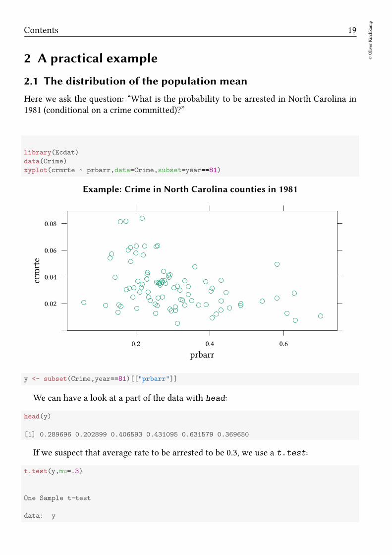
Here we ask the question: “What is the probability to be arrested in North Carolina in1981 (conditional on a crime committed)?”

library(Ecdat)

data(Crime)

xyplot(crmrte ~ prbarr,data=Crime,subset=year==81)

Example: Crime in North Carolina counties in 1981

prbarr

crmrte

0.02

0.04

0.06

0.08

0.2 0.4 0.6

y <- subset(Crime,year==81)[["prbarr"]]

We can have a look at a part of the data with head:

head(y)

[1] 0.289696 0.202899 0.406593 0.431095 0.631579 0.369650

If we suspect that average rate to be arrested to be 0.3, we use a t.test:

t.test(y,mu=.3)

One Sample t-test

data: y

20©Oliver

Kirchkam

p

13 August 2017 16:50:26

t = -0.070496, df = 89, p-value = 0.944

alternative hypothesis: true mean is not equal to 0.3

95 percent confidence interval:

0.2724894 0.3256254

sample estimates:

mean of x

0.2990574

An alternative: The Bayesian Approach Required:

• Priors for µ and τ.

• Likelihood: y ∼ N(µ, τ) with τ = 1/σ2

→ Posterior distribution of µ and τ.

We will here just “use” our software got get a result. Below we will explain what thesoftware actually does.

library(runjags)

X.model <- ’model

for (i in 1:length(y))

y[i] ~ dnorm(mu,tau)

mu ~ dnorm (0,.0001)

tau ~ dgamma(.01,.01)

sd <- sqrt(1/tau)

’

X.jags<-run.jags(model=X.model,data=list(y=y),monitor=c("mu","sd"))

Notation for nodes

• Stochastic nodes (discrete/continuous univariate/multivariate distributed):


...

mu ~ dnorm (0,.0001)

– . . . can be specified by data (have always this value)

– . . . can be specified by inits (have this value before the first sample)

– . . . can be unspecified

Note: if data or inits sets a value to NA, this means “unspecified”.

• Deterministic nodes:

Contents 21

©Oliver

Kirchkam

p

sd <- sqrt(1/tau)

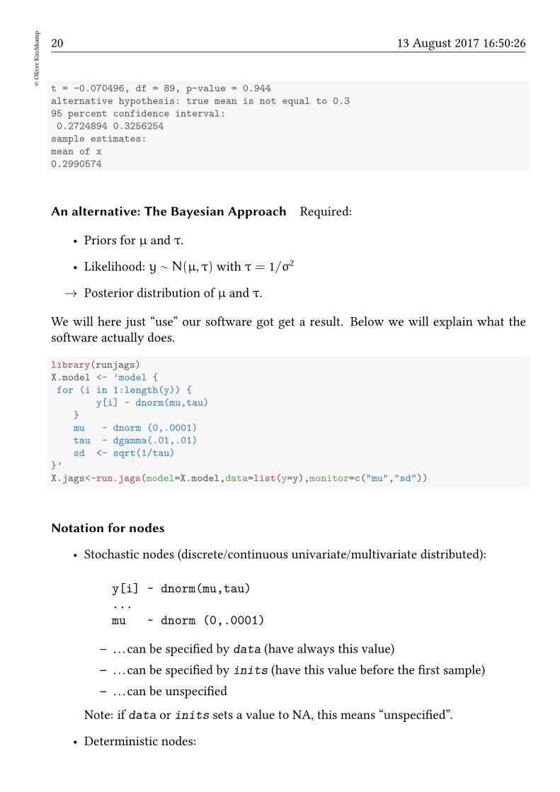
JAGS samples from the posterior of µ and τ. Here is a distribution for µ:

plot(X.jags,var="mu",plot.type=c("trace","density"))

Iteration

mu

0.26

0.30

0.34

6000 8000 10000 12000 14000

mu

Density

05

1015

2025

30

0.24 0.26 0.28 0.30 0.32 0.34 0.36

Here is a summary of our estimation results:

summary(X.jags)

Lower95 Median Upper95 Mean SD Mode MCerr

mu 0.272034 0.298984 0.325091 0.2990328 0.013468671 0.2986450 0.00009523789

sd 0.110458 0.128171 0.148288 0.1288285 0.009782551 0.1278104 0.00006969668

MC%ofSD SSeff AC.10 psrf

mu 0.7 20000 0.002831988 1.0000202

sd 0.7 19701 -0.003087232 0.9999656

Testing a point prediction in the t.test, as in µ = 0.3, is a bit strange, at least fromthe Bayesian perspective. It might be more interesting to make a statement about theprobability of an interval.First, we convert our jags-object into a dataframe: How probable is µ ∈ (0.29, 0.31)?

X.df<-data.frame(as.mcmc(X.jags))

str(X.df)

’data.frame’: 20000 obs. of 2 variables:

$ mu: num 0.331 0.289 0.316 0.317 0.303 ...

$ sd: num 0.126 0.119 0.116 0.122 0.118 ...

22©Oliver

Kirchkam

p

13 August 2017 16:50:26

We can now say, how probable it is, ex post, that µ ∈ [0.29, .31]:

100*mean(with(X.df,mu > 0.29 & mu < 0.31))

[1] 54.755

. . . or in a more narrow interval:


[1] 5.825


[1] 0.645

If, say, a government target is to have an average arrest rate of at least 0.25, we cannow calculate the probability that µ > 0.25.

How probable is µ > 0.25?

100*mean(with(X.df,mu > 0.25))

[1] 99.98

Odds for µ > 0.25

p<-mean(with(X.df,mu > 0.25))

p/(1-p)

[1] 4999

In the following section we will explain how all this works:

2.2 Gibbs sampling

The model that we specified above, contained two parts, a likelihood and a prior. Hereis a model with only a prior:

We use JAGS notation:dnorm(µ, τ)

with µ=mean and τ = 1/σ2=precision.

modelPri <- ’model

mu ~ dnorm (0,.0001)

’

Now we use this model to draw a sample of size 100, so far only given the prior.

Contents 23

©Oliver

Kirchkam

p

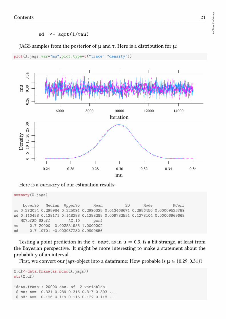
pri.jags<-run.jags(model=modelPri,monitor=c("mu"),sample=100)

Here are the properties of our sample:

summary(pri.jags)

Lower95 Median Upper95 Mean SD Mode MCerr MC%ofSD SSeff

mu -195.466 3.00919 169.874 -2.227341 98.9364 14.38885 8.278946 8.4 143

AC.10 psrf

mu 0.1140479 1.005316

And here is a plot of the distribution. Since we did not include a likelihood, it is at thesame time the distribution of the prior and of the posterior.

plot(pri.jags,var="mu",plot.type=c("trace","density"))

Iteration

mu

-300

-100

100

5000 5020 5040 5060 5080 5100

mu

Density

0.000

0.002

0.004

-400 -200 0 200

2.3 Convergence

In the sample above we saw only observations after round 5000, i.e. we skipped 5000samples of adaptation and burnin. This was not necessary, since we had only a prior,i.e. the sampler would only sample from the prior.

Things become more interesting when we add a likelihood (which we will do next).Then it is not clear that the sampler will directly start sampling from the posterior distri-bution. It takes some time. The hope is that after 5000 samples of adaptation and burnin

24©Oliver

Kirchkam

p

13 August 2017 16:50:26

the sampler has converged, that it samples from an almost stationary distribution (whichis described by our prior and our likelihood).

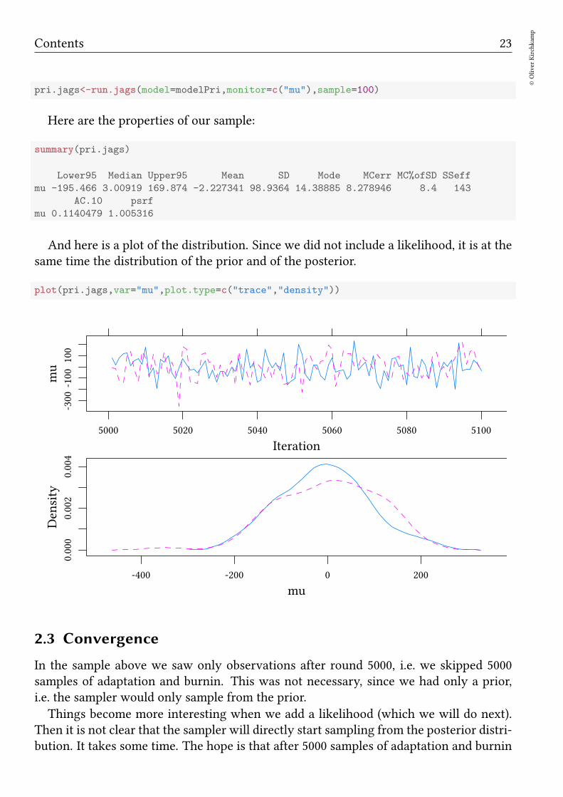
In the following we add the likelihood to the model. We drop adaptation and burninand see what happens at the start.

ini<-genInit(2,function(i) list(mu=c(100,-100)[i]))

X2.model <- ’model



mu ~ dnorm (200,.0001)


sd <- sqrt(1/tau)

’

X100.jags<-run.jags(model=X2.model,data=list(y=y),

monitor=c("mu","sd"),adapt=0,burnin=0,sample=100,inits=ini)

(To obtain reproducible results, I use a custom genInit function in this handout. Youfind this function in the attachment to this document. You also find a definition in Section16. For you own calculations you can also drop the inits=ini part.)

plot(X100.jags,var="mu",plot.type=c("trace"))

Iteration

mu

0.25

0.30

0.35

0 20 40 60 80 100

At least here the sampler seems to converge fast. Nevertheless, including a safe numberof adaptation and burnin is good practice. Let us look at the posterior with adaptationand burnin:

Contents 25

©Oliver

Kirchkam

p

X1001.jags<-run.jags(model=X2.model,data=list(y=y),monitor=c("mu","sd"),

inits=ini)

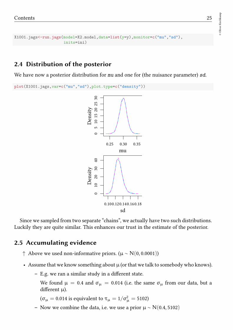
2.4 Distribution of the posterior

We have now a posterior distribution for mu and one for (the nuisance parameter) sd.

plot(X1001.jags,var=c("mu","sd"),plot.type=c("density"))

mu

Density

05

1015

2025

30

0.25 0.30 0.35

sd

Density

010

2030

40

0.100.120.140.160.18

Since we sampled from two separate “chains”, we actually have two such distributions.Luckily they are quite similar. This enhances our trust in the estimate of the posterior.

2.5 Accumulating evidence

↑ Above we used non-informative priors. (µ ∼ N(0, 0.0001))

• Assume thatwe know something aboutµ (or thatwe talk to somebodywho knows).

– E.g. we ran a similar study in a different state.

We found µ = 0.4 and σµ = 0.014 (i.e. the same σµ from our data, but adifferent µ).

(σµ = 0.014 is equivalent to τµ = 1/σ2µ = 5102)

– Now we combine the data, i.e. we use a prior µ ∼ N(0.4, 5102)

26©Oliver

Kirchkam

p

13 August 2017 16:50:26

XA.model <- ’model



mu ~ dnorm (0.4,1/0.014^2)


sd <- sqrt(1/tau)

’

XA.jags<-run.jags(model=XA.model,data=list(y=y),monitor=c("mu","sd"))

summary(XA.jags)


mu 0.329932 0.3514325 0.372681 0.3516260 0.01084617 0.3515811 0.00008563219

sd 0.117564 0.1381880 0.161305 0.1390088 0.01128897 0.1372491 0.00008957363


mu 0.8 16043 0.002953220 0.9999910

sd 0.8 15884 0.006200908 0.9999954

• Prior mean: 0.4

• Sample mean: 0.3

• Posterior mean: 0.35

“A Bayesian is one who, vaguely expecting a horse, and catching a glimpse of a donkey,strongly believes he has seen a mule.”

2.6 Priors

• noninformative, flat, vague, diffuse

• weakly informative: intentionally weaker than the available prior knowledge, tokeep the parameter within “reasonable bounds”.

• informative: available prior knowledge.

3 Conjugate Priors

3.1 Accumulating evidence, continued

ExchangabilityWhen we accumulate data X1 and X2 it should not matter, whether we first observe X1

and then add X2 or vice versa.

Call D the distribution of parameter θ.

Contents 27

©Oliver

Kirchkam

p

D0X1−→ D1

X2−→ D12

D0X2−→ D2

X1−→ D12

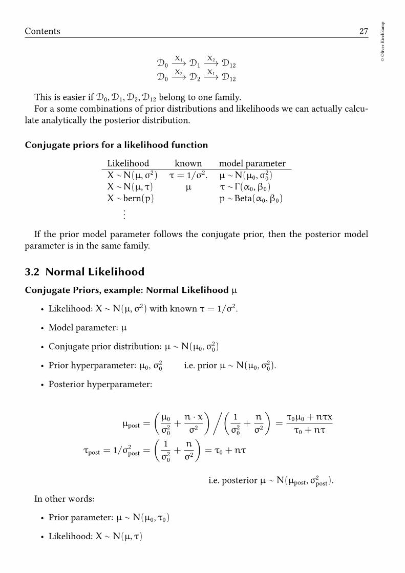
This is easier if D0,D1,D2,D12 belong to one family.For a some combinations of prior distributions and likelihoods we can actually calcu-

late analytically the posterior distribution.

Conjugate priors for a likelihood function

Likelihood known model parameter

X ∼N(µ,σ2) τ = 1/σ2. µ ∼N(µ0,σ20)

X ∼N(µ, τ) µ τ ∼ Γ(α0,β0)

X ∼ bern(p) p ∼Beta(α0,β0)...

If the prior model parameter follows the conjugate prior, then the posterior modelparameter is in the same family.

3.2 Normal Likelihood

Conjugate Priors, example: Normal Likelihood µ

• Likelihood: X ∼ N(µ,σ2) with known τ = 1/σ2.

• Model parameter: µ

• Conjugate prior distribution: µ ∼ N(µ0,σ20)

• Prior hyperparameter: µ0, σ20 i.e. prior µ ∼ N(µ0,σ

20).

• Posterior hyperparameter:

µpost =

(

µ0

σ20+n · xσ2

)/(

1

σ20+n

σ2

)

=τ0µ0 + nτx

τ0 + nτ

τpost = 1/σ2post =

(

1

σ20+n

σ2

)

= τ0 + nτ

i.e. posterior µ ∼ N(µpost,σ2post).

In other words:

• Prior parameter: µ ∼ N(µ0, τ0)

• Likelihood: X ∼ N(µ, τ)

28©Oliver

Kirchkam

p

13 August 2017 16:50:26

• Posterior parameter: µ ∼ N(µpost, τpost).

Terminology:

• Hyperparameters: µ0, τ0 (they determine the distribution of µ)

• Parameters: µ, τ

• Posterior hyperparameters: µpost, τpost

Conjugate Priors, example: Normal Likelihood τ

• Likelihood: X ∼ N(µ, τ) with known µ.

• Model parameter: τ = 1/σ2

• Conjugate prior distribution: τ ∼ Γ(α0,β0)

• Prior hyperparameter: α0, β0


shape αpost = α0 +n

2

rate βpost = β0 +n

2var(x)

In other words:

• Prior parameter: τ ∼ Γ(α0,β0)

• Likelihood: X ∼ N(µ, τ)

• Posterior parameter: τ ∼ Γ(αpost,βpost).

Terminology:

• Hyperparameters: α0,β0 (they determine the distribution of µ)


• Posterior hyperparameters: αpost,βpost

Contents 29

©Oliver

Kirchkam

p

3.3 Bernoulli Likelihood

Conjugate Priors, example: Bernoulli Likelihood

• Likelihood: X ∼ bern(p).

• Model parameter: p

• Conjugate prior distribution: p ∼ Beta(α0,β0)

• Prior hyperparameter: α0, β0


αpost = α0 +∑

xi

βpost = β0 + n−∑

xi

In other words:

• Prior parameter: p ∼ Beta(α0,β0)

• Likelihood: X ∼ bern(p)

• Posterior parameter: p ∼ Beta(αpost,βpost)

Terminology:

• Hyperparameters: α0,β0 (they determine the distribution of µ)


• Posterior hyperparameters: αpost,βpost

3.4 Problems with the analytical approach

• Restrictive for. . .

– priors

– likelihood (“the model” in the frequentist world)

• For many relevant cases we have no analytical solution.

• → numerical methods, Markov Chain Monte Carlo (MCMC) methods, Metropolis-Hastings sampling, Gibbs sampling,. . .

Construct a Markov Chain that has the posterior distribution as its equilibrium distri-bution.

30©Oliver

Kirchkam

p

13 August 2017 16:50:26

3.5 Exercises

1. An event can have two possible outcomes, 0 or 1. You are interested in the proba-bility p of obtaining a 1. You assume that p follows a Beta distribution. Your prioris that the parameters of the Beta distribution are α = β = 0. You observe threetimes a 1 and no 0. What is your posterior for α and β?

2. Later you observe three more times a 1 and four times 0. Given all your observa-tions, what is now your posterior for α and β?

3. A random variable X follows a normal distribution with mean µ and precision τ.You want to infer the posterior distribution of µ. Your prior for µ also follows anormal distribution µ ∼ N(µ0, τ0) with hyperparameters µ0 = 10 and τ0 = 2.Now you observe a sample of size n = 10, mean µ = 20 and precision τ = 1/5.What is your posterior µpost?

4. What is your posterior τpost

4 Linear Regression

We use linear regression as an example to illustrate some issues of the mechanics behindthe MCMC sampling mentioned in the previous section.

4.1 Introduction

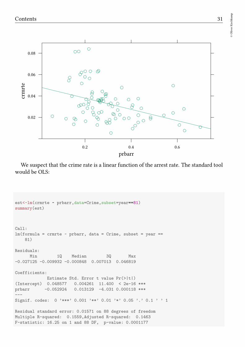
Example: Crime in North Carolina in 1981 Let us have another look at the crimerate and the arrest rate in North Carolina.

library(Ecdat)

data(Crime)

xyplot(crmrte ~ prbarr,data=Crime,subset=year==81,type=c("p","r"))

Contents 31

©Oliver

Kirchkam

p

prbarr

crmrte

0.02

0.04

0.06

0.08

0.2 0.4 0.6

We suspect that the crime rate is a linear function of the arrest rate. The standard toolwould be OLS:

est<-lm(crmrte ~ prbarr,data=Crime,subset=year==81)

summary(est)

Call:

lm(formula = crmrte ~ prbarr, data = Crime, subset = year ==

81)

Residuals:

Min 1Q Median 3Q Max

-0.027125 -0.009932 -0.000848 0.007013 0.046819

Coefficients:

Estimate Std. Error t value Pr(>|t|)

(Intercept) 0.048577 0.004261 11.400 < 2e-16 ***

prbarr -0.052924 0.013129 -4.031 0.000118 ***

---

Signif. codes: 0 ’***’ 0.001 ’**’ 0.01 ’*’ 0.05 ’.’ 0.1 ’ ’ 1

Residual standard error: 0.01571 on 88 degrees of freedom

Multiple R-squared: 0.1559,Adjusted R-squared: 0.1463

F-statistic: 16.25 on 1 and 88 DF, p-value: 0.0001177

32©Oliver

Kirchkam

p

13 August 2017 16:50:26

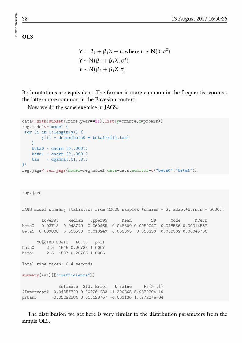
OLS

Y = β0 + β1X+ u where u ∼ N(0,σ2)

Y ∼ N(β0 + β1X,σ2)

Y ∼ N(β0 + β1X, τ)

Both notations are equivalent. The former is more common in the frequentist context,the latter more common in the Bayesian context.

Now we do the same exercise in JAGS:

data<-with(subset(Crime,year==81),list(y=crmrte,x=prbarr))

reg.model<-’model


y[i] ~ dnorm(beta0 + beta1*x[i],tau)

beta0 ~ dnorm (0,.0001)

beta1 ~ dnorm (0,.0001)


’

reg.jags<-run.jags(model=reg.model,data=data,monitor=c("beta0","beta1"))

reg.jags

JAGS model summary statistics from 20000 samples (chains = 2; adapt+burnin = 5000):


beta0 0.03718 0.048729 0.060465 0.048809 0.0059047 0.048566 0.00014557

beta1 -0.089838 -0.053553 -0.018249 -0.053655 0.018233 -0.053532 0.00045766


beta0 2.5 1645 0.20733 1.0007

beta1 2.5 1587 0.20768 1.0006

Total time taken: 0.4 seconds

summary(est)[["coefficients"]]


(Intercept) 0.04857749 0.004261233 11.399865 5.087079e-19

prbarr -0.05292384 0.013128767 -4.031136 1.177237e-04

The distribution we get here is very similar to the distribution parameters from thesimple OLS.

Contents 33

©Oliver

Kirchkam

p

4.2 Demeaning

This is a technical issue. Demeaning might help improving the performance of our sam-pler.

Demeaning does not change the estimate of the coefficient of X, it does change theconstant, though.

Y = β0 + β1X (1)

Y − Y = β0 − Y + β1X︸︷︷︸β′

0

+β1(X− X) (2)

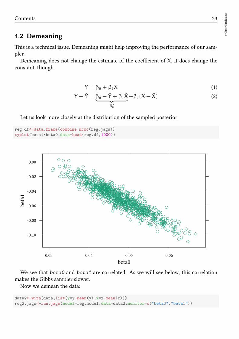
Let us look more closely at the distribution of the sampled posterior:

reg.df<-data.frame(combine.mcmc(reg.jags))

xyplot(beta1~beta0,data=head(reg.df,1000))

beta0

beta1

-0.10

-0.08

-0.06

-0.04

-0.02

0.00

0.03 0.04 0.05 0.06

We see that beta0 and beta1 are correlated. As we will see below, this correlationmakes the Gibbs sampler slower.

Now we demean the data:

data2<-with(data,list(y=y-mean(y),x=x-mean(x)))

reg2.jags<-run.jags(model=reg.model,data=data2,monitor=c("beta0","beta1"))

34©Oliver

Kirchkam

p

13 August 2017 16:50:26

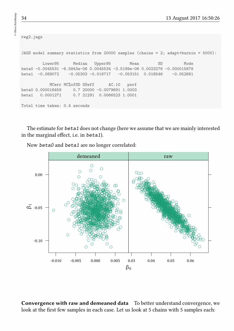
reg2.jags


Lower95 Median Upper95 Mean SD Mode

beta0 -0.0045531 -6.5843e-06 0.0045534 -3.5199e-06 0.0023276 -0.000015878

beta1 -0.089072 -0.05303 -0.016717 -0.053151 0.018546 -0.052681

MCerr MC%ofSD SSeff AC.10 psrf

beta0 0.000016459 0.7 20000 -0.0079691 1.0003

beta1 0.0001271 0.7 21291 0.0066523 1.0001


The estimate for beta1 does not change (here we assume that we aremainly interestedin the marginal effect, i.e. in beta1).

Now beta0 and beta1 are no longer correlated:

β0

β1

-0.10

-0.05

0.00

-0.010 -0.005 0.000 0.005

demeaned

0.03 0.04 0.05 0.06

raw

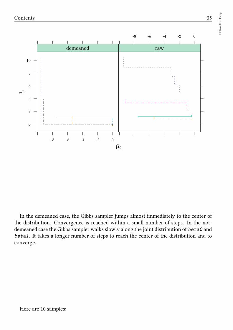
Convergence with raw and demeaned data To better understand convergence, welook at the first few samples in each case. Let us look at 5 chains with 5 samples each:

Contents 35

©Oliver

Kirchkam

p

β0

β1

0

2

4

6

8

10

-8 -6 -4 -2 0

demeaned

-8 -6 -4 -2 0

raw

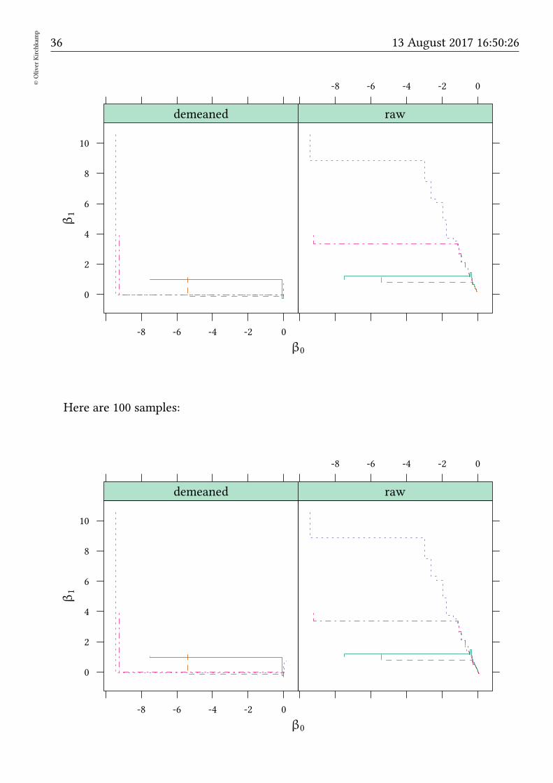
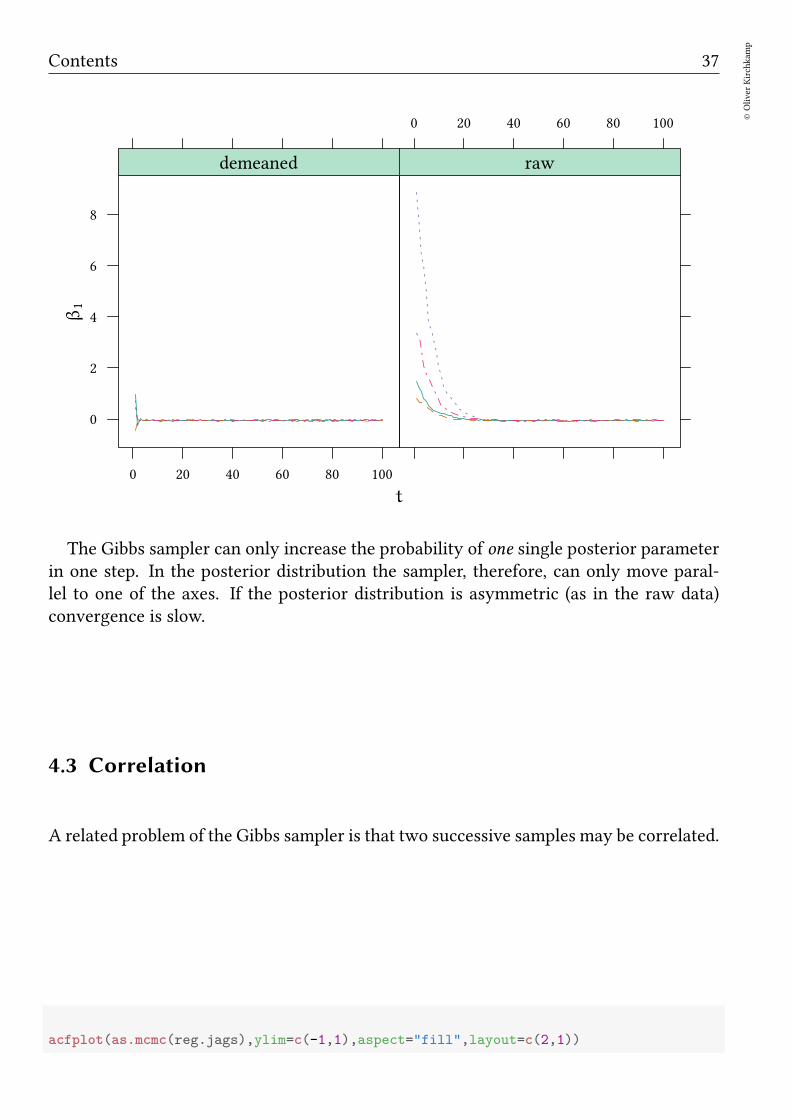
In the demeaned case, the Gibbs sampler jumps almost immediately to the center ofthe distribution. Convergence is reached within a small number of steps. In the not-demeaned case the Gibbs sampler walks slowly along the joint distribution of beta0 andbeta1. It takes a longer number of steps to reach the center of the distribution and toconverge.

Here are 10 samples:

36©Oliver

Kirchkam

p

13 August 2017 16:50:26

β0

β1

0

2

4

6

8

10

-8 -6 -4 -2 0

demeaned

-8 -6 -4 -2 0

raw

Here are 100 samples:

β0

β1

0

2

4

6

8

10

-8 -6 -4 -2 0

demeaned

-8 -6 -4 -2 0

raw

Contents 37

©Oliver

Kirchkam

p

t

β1

0

2

4

6

8

0 20 40 60 80 100

demeaned

0 20 40 60 80 100

raw

The Gibbs sampler can only increase the probability of one single posterior parameterin one step. In the posterior distribution the sampler, therefore, can only move paral-lel to one of the axes. If the posterior distribution is asymmetric (as in the raw data)convergence is slow.

4.3 Correlation

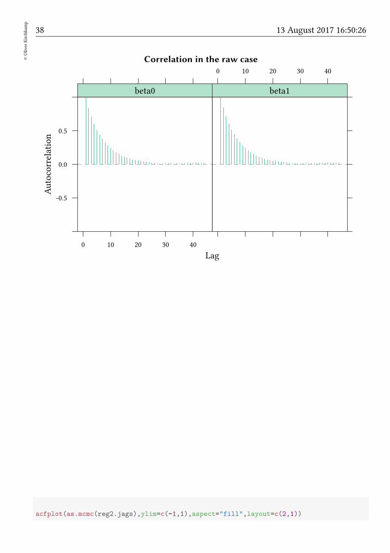
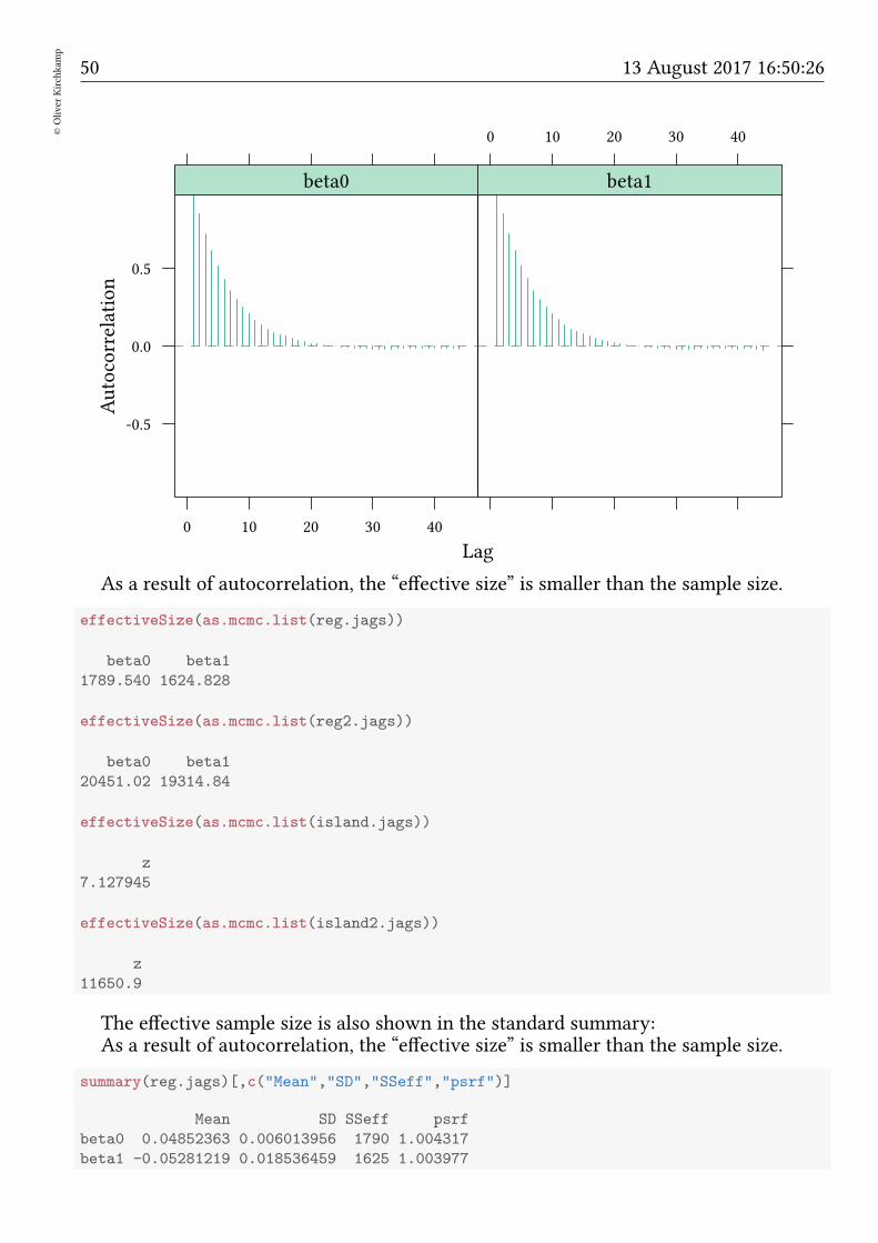
A related problem of the Gibbs sampler is that two successive samples may be correlated.

acfplot(as.mcmc(reg.jags),ylim=c(-1,1),aspect="fill",layout=c(2,1))

38©Oliver

Kirchkam

p

13 August 2017 16:50:26

Correlation in the raw case

Lag

Autocorrelation

-0.5

0.0

0.5

0 10 20 30 40

beta0

0 10 20 30 40

beta1

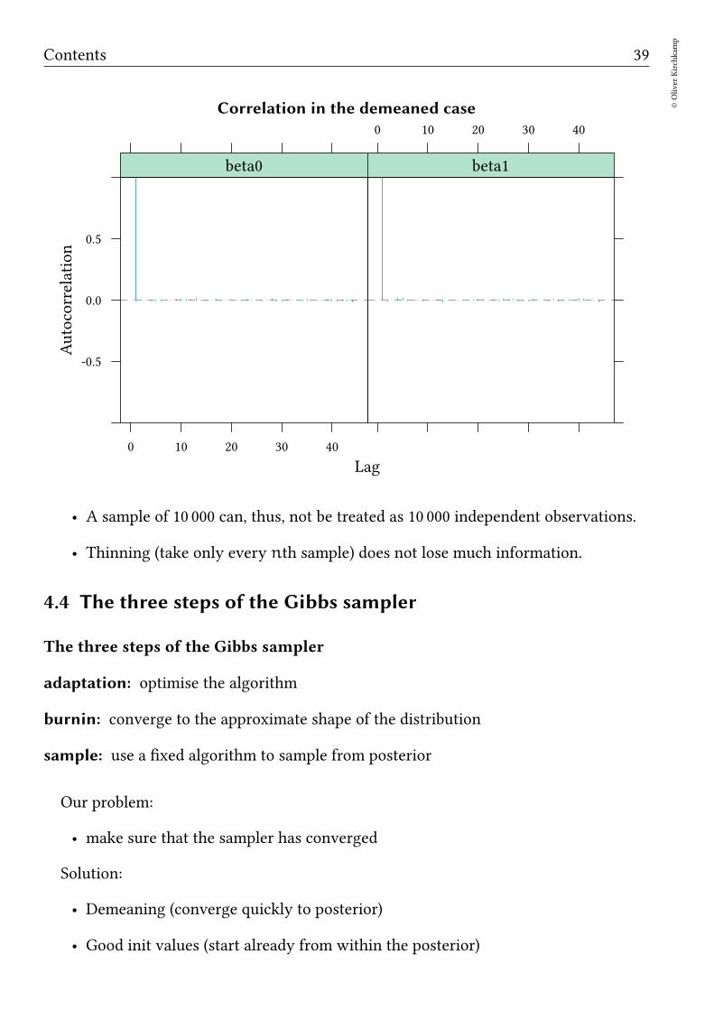
acfplot(as.mcmc(reg2.jags),ylim=c(-1,1),aspect="fill",layout=c(2,1))

Contents 39

©Oliver

Kirchkam

p

Correlation in the demeaned case

Lag

Autocorrelation

-0.5

0.0

0.5

0 10 20 30 40

beta0

0 10 20 30 40

beta1

• A sample of 10 000 can, thus, not be treated as 10 000 independent observations.

• Thinning (take only every nth sample) does not lose much information.

4.4 The three steps of the Gibbs sampler

The three steps of the Gibbs sampler

adaptation: optimise the algorithm

burnin: converge to the approximate shape of the distribution

sample: use a fixed algorithm to sample from posterior

Our problem:

• make sure that the sampler has converged

Solution:

• Demeaning (converge quickly to posterior)

• Good init values (start already from within the posterior)

40©Oliver

Kirchkam

p

13 August 2017 16:50:26

4.5 Exercises

Consider the year 1979 from the data set LaborSupply from Ecdat.

1. Which variables could explain labor supply?

2. Estimate your model for the year 1979 only.

3. Compare your results with and without demeaning.

5 Finding posteriors

5.1 Overview



· 1

Pr(X)︸︷︷︸

∫Pr(θ)·Pr(X|θ)dθ


Find Pr(θ|X):

• Exact: but∫Pr(θ) · Pr(X|θ)dθ can be hard (except for specific priors and likeli-

hoods).

• MCMC Sampling

– Rejection sampling: can be very slow (for a high-dimensional problem, andour problems are high-dimensional).

– Metropolis–Hastings: quicker, samples are correlated, requires sampling of θfrom joint distribution Pr(X|θ).

– Gibbs sampling: quicker, samples are correlated, requires sampling of θi fromconditional (on θ−i) distribution Pr(X|θi, θ−i).

→ this is easy! (at least much easier than Pr(X|θ))

5.2 Example for the exact way:

Above we talked about conjugate priors. Consider the case of Normal Likelihood:

• Likelihood: N(µ,σ2) with known τ = 1/σ2.

• Model parameter: µ

• Conjugate prior distribution: µ ∼ N()

• Prior hyperparameter: µ0, σ20

Contents 41

©Oliver

Kirchkam

p


µpost =

(

µ0

σ20+n · xσ2

)/(

1

σ20+n

σ2

)

=τ0µ0 + nτx

τ0 + nτ

τpost = 1/σ2post =

(

1

σ20+n

σ2

)

= τ0 + nτ

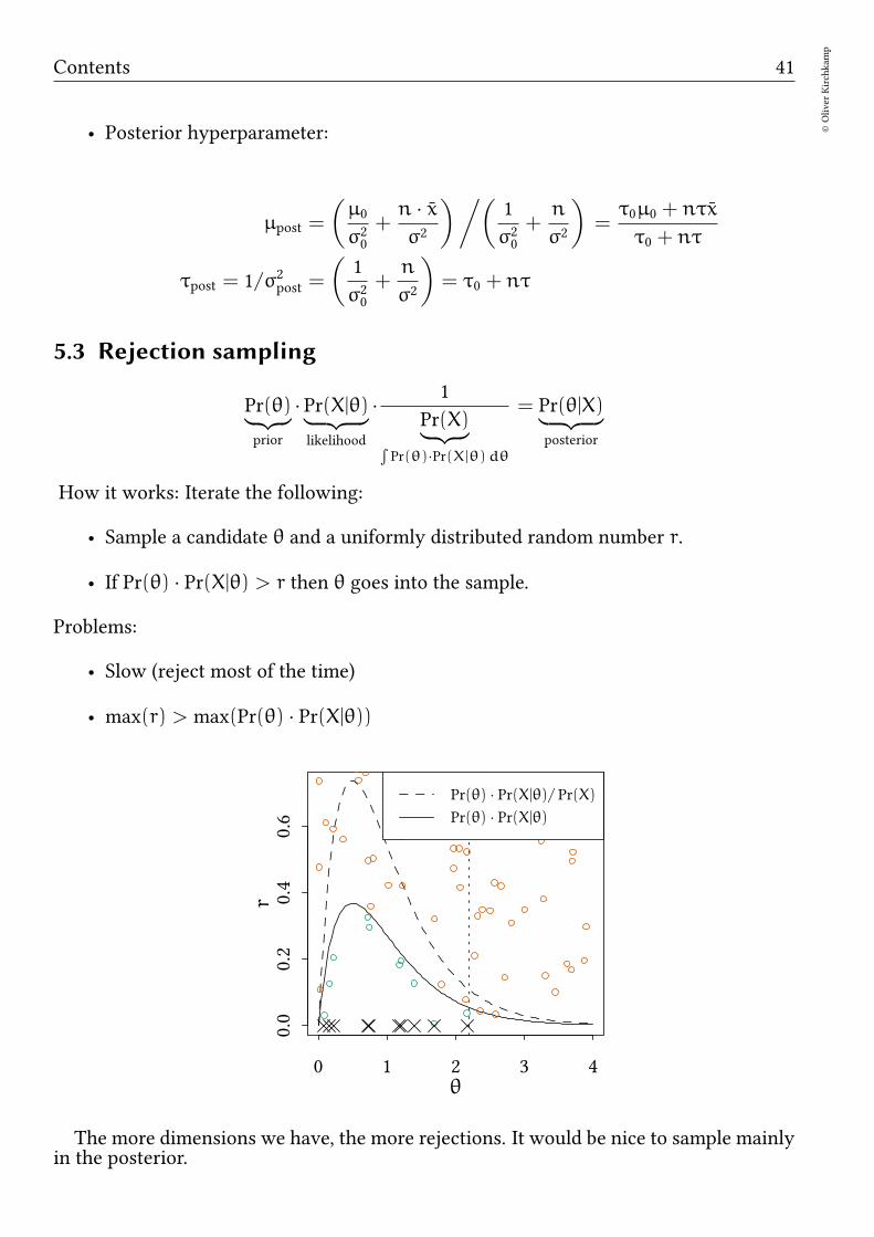
5.3 Rejection sampling



· 1

Pr(X)︸︷︷︸



How it works: Iterate the following:

• Sample a candidate θ and a uniformly distributed random number r.

• If Pr(θ) · Pr(X|θ) > r then θ goes into the sample.

Problems:

• Slow (reject most of the time)

• max(r) > max(Pr(θ) · Pr(X|θ))

0 1 2 3 4

0.0

0.2

0.4

0.6

θ

r

Pr(θ) · Pr(X|θ)/ Pr(X)Pr(θ) · Pr(X|θ)

The more dimensions we have, the more rejections. It would be nice to sample mainlyin the posterior.

42©Oliver

Kirchkam

p

13 August 2017 16:50:26

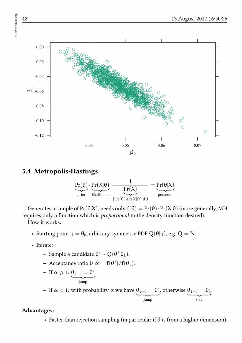
β0

β1

-0.12

-0.10

-0.08

-0.06

-0.04

-0.02

0.00

0.04 0.05 0.06 0.07

5.4 Metropolis-Hastings



· 1

Pr(X)︸︷︷︸



Generates a sample of Pr(θ|X), needs only f(θ) = Pr(θ) ·Pr(X|θ) (more generally, MHrequires only a function which is proportional to the density function desired).How it works:

• Starting point η = θ0, arbitrary symmetric PDF Q(θ|η), e.g. Q = N.

• Iterate:

– Sample a candidate θ ′ ∼ Q(θ ′|θt).

– Acceptance ratio is α = f(θ ′)/f(θt).

– If α > 1: θt+1 = θ′

︸︷︷︸jump

– If α < 1: with probability α we have θt+1 = θ′

︸︷︷︸jump

, otherwise θt+1 = θt︸︷︷︸

stay

.

Advantages:

• Faster than rejection sampling (in particular if θ is from a higher dimension).

Contents 43

©Oliver

Kirchkam

p

Disadvantages:

• Samples are correlated (depending on Q).

– If Q makes wide jumps: more rejections but less correlation.

– If Q makes small jumps: fewer rejections but more correlation.

• Initial samples are from a different distribution. “burn-in” required.

• Finding a “good” jumping distribution Q(x|y) can be tricky.

5.5 Gibbs sampling

Essentially as in Metropolis-Hastings, except that sampling is performed for each com-ponent of θ sequentially.

• determine θt+11 with f(θ1|θ

t2 , θ

t3 , θ

t4 , . . . , θ

tn)


t+11 , θt3 , θ

t4 , . . . , θ

tn)


t+11 , θt+1

2 , θt4 , . . . , θtn)

•...

• determine θt+1n with f(θn|θ

t+11 , θt+1

2 , . . . , θt+1n−1)

Advantages:

• Requires only conditional distributions. f(θi|θ−1), not joint distributions.

• Finding a “good” jumping distribution Q(x|y) is easier.

Disadvantages:

• Samples are correlated (potentially more than in MH if the number of dimen-sions is large).

• Initial samples are from a different distribution. “burn-in” required.

• Can get stuck on “unconnected islands”.

44©Oliver

Kirchkam

p

13 August 2017 16:50:26

0.0 0.2 0.4 0.6 0.8 1.0

0.0

0.2

0.4

0.6

0.8

1.0

θ1

θ2

P = 1/2

P = 1/2

In the following example we create on purpose a situation with two (almost) uncon-nected islands:

x<-rbinom(9,1,.5)

x

[1] 0 0 0 1 0 1 0 0 0

island.mod<-’model

for (i in 1:length(x))

x[i] ~ dbern(z^2)

z ~ dunif(-1,1)

’

island.jags<-run.jags(model=island.mod,data=list(x=x),monitor=c("z"),

inits=ini)

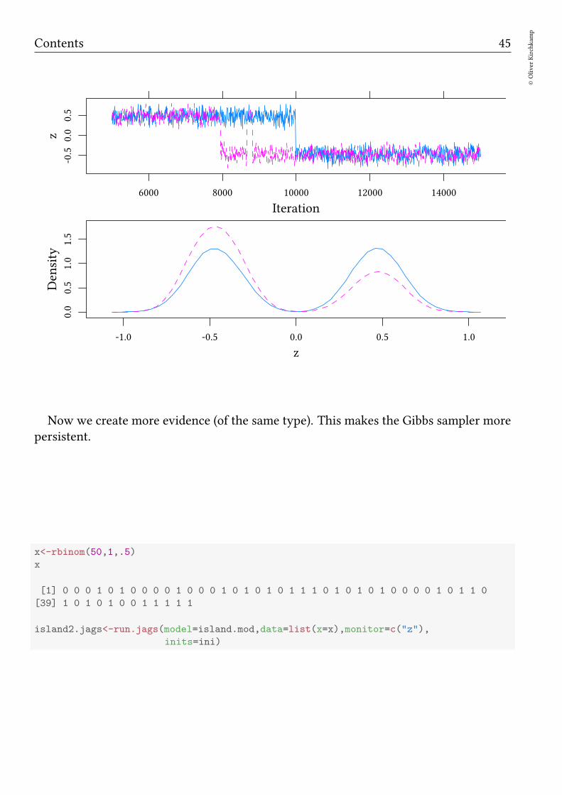
Contents 45

©Oliver

Kirchkam

p

Iteration

z-0.5

0.0

0.5

6000 8000 10000 12000 14000

z

Density

0.0

0.5

1.0

1.5

-1.0 -0.5 0.0 0.5 1.0

Now we create more evidence (of the same type). This makes the Gibbs sampler morepersistent.

x<-rbinom(50,1,.5)

x

[1] 0 0 0 1 0 1 0 0 0 0 1 0 0 0 1 0 1 0 1 0 1 1 1 0 1 0 1 0 1 0 0 0 0 1 0 1 1 0

[39] 1 0 1 0 1 0 0 1 1 1 1 1

island2.jags<-run.jags(model=island.mod,data=list(x=x),monitor=c("z"),

inits=ini)

46©Oliver

Kirchkam

p

13 August 2017 16:50:26

Iteration

z-0.5

0.0

0.5

6000 8000 10000 12000 14000

z

Density

02

46

8

-0.5 0.0 0.5

5.6 Check convergence

5.6.1 Gelman, Rubin (1992): potential scale reduction factor

Idea: take k chains, discard “warm-up”, split remaining chains, so that we have 2k se-quences ψ, each of length n.

B = between sequence variance

W = within sequence variance

Variance of all chains combined:

σ2 =n− 1

nW +

B

n

Potential scale reduction:

R =

√

σ2

W

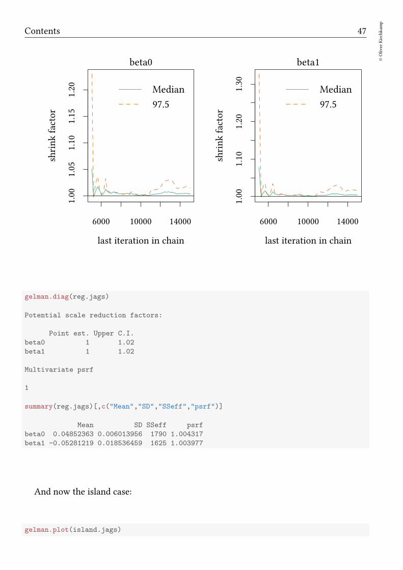
Let us first look at the psrf for a “nice” case:

gelman.plot(reg.jags)

Contents 47

©Oliver

Kirchkam

p

6000 10000 14000

1.00

1.05

1.10

1.15

1.20

last iteration in chain

shrinkfactor

Median

97.5

beta0

6000 10000 14000

1.00

1.10

1.20

1.30


shrinkfactor

Median

97.5

beta1

gelman.diag(reg.jags)

Potential scale reduction factors:

Point est. Upper C.I.

beta0 1 1.02

beta1 1 1.02

Multivariate psrf

1

summary(reg.jags)[,c("Mean","SD","SSeff","psrf")]

Mean SD SSeff psrf

beta0 0.04852363 0.006013956 1790 1.004317

beta1 -0.05281219 0.018536459 1625 1.003977

And now the island case:

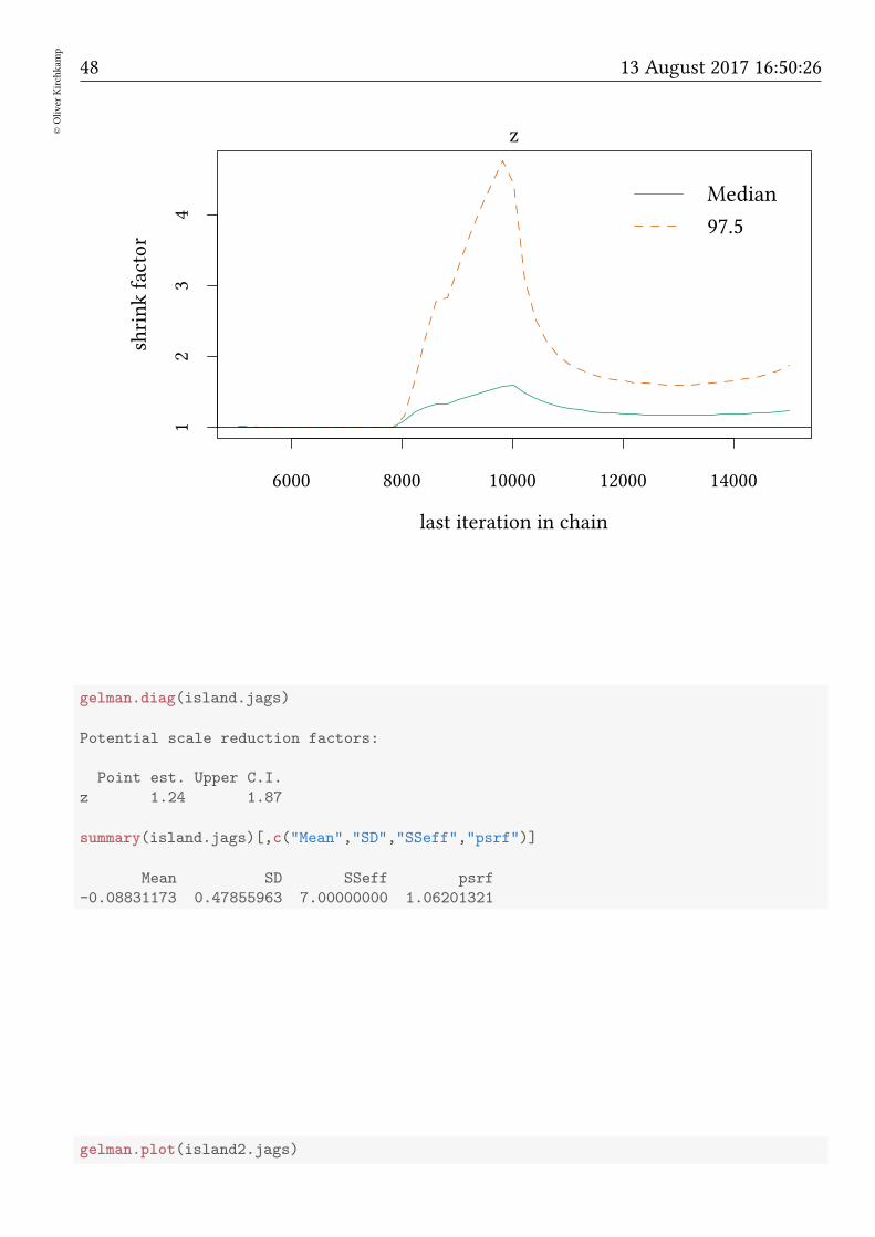
gelman.plot(island.jags)

48©Oliver

Kirchkam

p

13 August 2017 16:50:26

6000 8000 10000 12000 14000

12

34


shrinkfactor

Median

97.5

z

gelman.diag(island.jags)



z 1.24 1.87

summary(island.jags)[,c("Mean","SD","SSeff","psrf")]

Mean SD SSeff psrf

-0.08831173 0.47855963 7.00000000 1.06201321

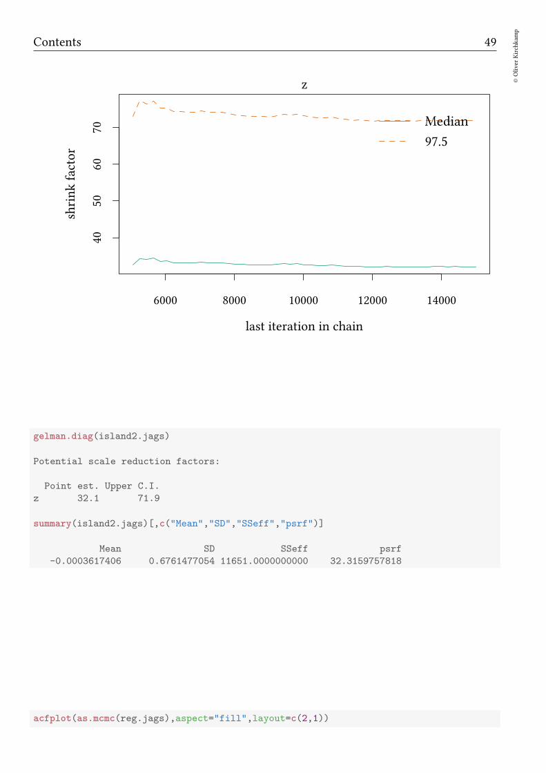
gelman.plot(island2.jags)

Contents 49

©Oliver

Kirchkam

p

6000 8000 10000 12000 14000

4050

6070


shrinkfactor

Median

97.5

z

gelman.diag(island2.jags)



z 32.1 71.9

summary(island2.jags)[,c("Mean","SD","SSeff","psrf")]

Mean SD SSeff psrf

-0.0003617406 0.6761477054 11651.0000000000 32.3159757818

acfplot(as.mcmc(reg.jags),aspect="fill",layout=c(2,1))

50©Oliver

Kirchkam

p

13 August 2017 16:50:26

Lag

Autocorrelation

-0.5

0.0

0.5

0 10 20 30 40

beta0

0 10 20 30 40

beta1

As a result of autocorrelation, the “effective size” is smaller than the sample size.

effectiveSize(as.mcmc.list(reg.jags))

beta0 beta1

1789.540 1624.828

effectiveSize(as.mcmc.list(reg2.jags))

beta0 beta1

20451.02 19314.84

effectiveSize(as.mcmc.list(island.jags))

z

7.127945

effectiveSize(as.mcmc.list(island2.jags))

z

11650.9

The effective sample size is also shown in the standard summary:As a result of autocorrelation, the “effective size” is smaller than the sample size.

summary(reg.jags)[,c("Mean","SD","SSeff","psrf")]

Mean SD SSeff psrf

beta0 0.04852363 0.006013956 1790 1.004317

beta1 -0.05281219 0.018536459 1625 1.003977

Contents 51

©Oliver

Kirchkam

p

summary(reg2.jags)[,c("Mean","SD","SSeff","psrf")]

Mean SD SSeff psrf

beta0 0.000002490592 0.002313587 20451 1.000003

beta1 -0.052811075786 0.018378246 19315 1.000053

summary(island.jags)[,c("Mean","SD","SSeff","psrf")]

Mean SD SSeff psrf

-0.08831173 0.47855963 7.00000000 1.06201321

summary(island2.jags)[,c("Mean","SD","SSeff","psrf")]

Mean SD SSeff psrf

-0.0003617406 0.6761477054 11651.0000000000 32.3159757818

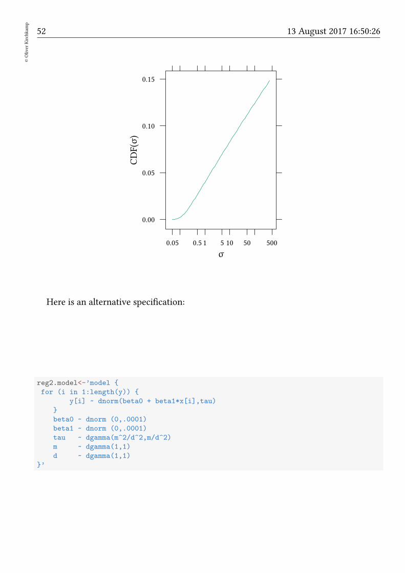
5.7 A beer vague prior for τ

When we specify a regression model we need a precision parameter τ. So far we did this:

reg.model<-’model



beta0 ~ dnorm (0,.0001)

beta1 ~ dnorm (0,.0001)


’

52©Oliver

Kirchkam

p

13 August 2017 16:50:26

σ

CDF(σ)

0.00

0.05

0.10

0.15

0.05 0.5 1 5 10 50 500

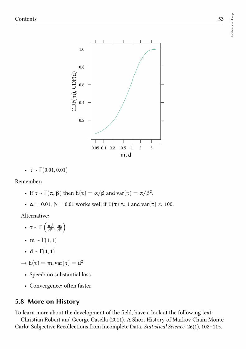
Here is an alternative specification:

reg2.model<-’model



beta0 ~ dnorm (0,.0001)

beta1 ~ dnorm (0,.0001)

tau ~ dgamma(m^2/d^2,m/d^2)

m ~ dgamma(1,1)

d ~ dgamma(1,1)

’

Contents 53

©Oliver

Kirchkam

p

m,d

CDF(m),CDF(d)

0.2

0.4

0.6

0.8

1.0

0.05 0.1 0.2 0.5 1 2 5

• τ ∼ Γ(0.01, 0.01)

Remember:

• If τ ∼ Γ(α,β) then E(τ) = α/β and var(τ) = α/β2.

• α = 0.01, β = 0.01 works well if E(τ) ≈ 1 and var(τ) ≈ 100.

Alternative:

• τ ∼ Γ(

m2

d2 ,md2

)

• m ∼ Γ(1, 1)

• d ∼ Γ(1, 1)

→ E(τ) = m, var(τ) = d2

• Speed: no substantial loss

• Convergence: often faster

5.8 More on History

To learn more about the development of the field, have a look at the following text:Christian Robert and George Casella (2011). A Short History of Markov Chain Monte

Carlo: Subjective Recollections from Incomplete Data. Statistical Science. 26(1), 102–115.

54©Oliver

Kirchkam

p

13 August 2017 16:50:26

6 Robust regression

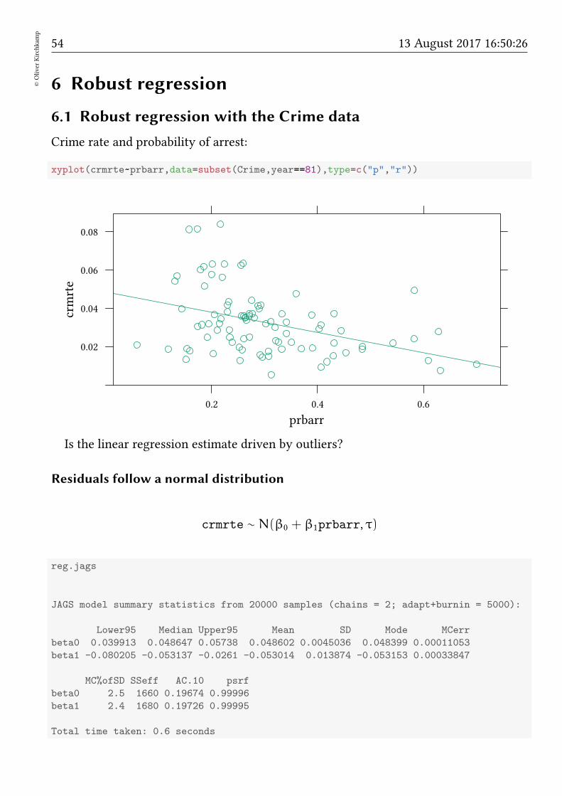
6.1 Robust regression with the Crime data

Crime rate and probability of arrest:

xyplot(crmrte~prbarr,data=subset(Crime,year==81),type=c("p","r"))

prbarr

crmrte

0.02

0.04

0.06

0.08

0.2 0.4 0.6

Is the linear regression estimate driven by outliers?

Residuals follow a normal distribution

crmrte ∼ N(β0 + β1prbarr, τ)

reg.jags



beta0 0.039913 0.048647 0.05738 0.048602 0.0045036 0.048399 0.00011053

beta1 -0.080205 -0.053137 -0.0261 -0.053014 0.013874 -0.053153 0.00033847


beta0 2.5 1660 0.19674 0.99996

beta1 2.4 1680 0.19726 0.99995


Contents 55

©Oliver

Kirchkam

p

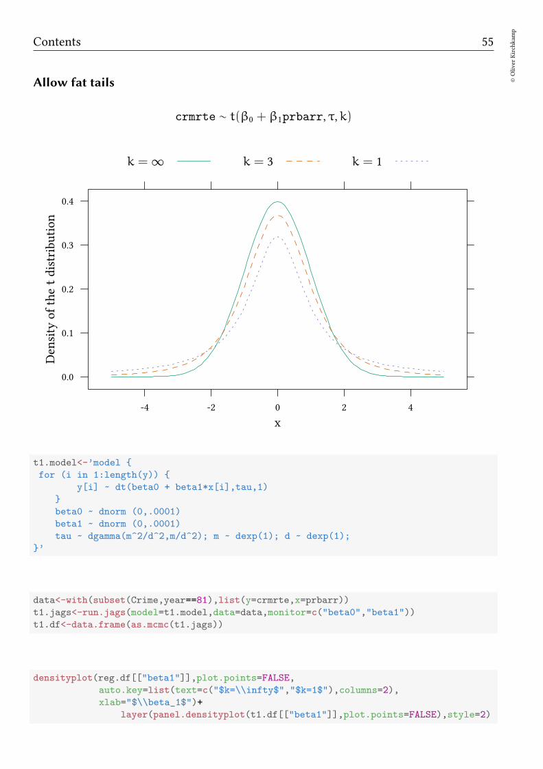
Allow fat tails

crmrte ∼ t(β0 + β1prbarr, τ,k)

x

Density

ofthetdistribution

0.0

0.1

0.2

0.3

0.4

-4 -2 0 2 4

k = ∞ k = 3 k = 1

t1.model<-’model


y[i] ~ dt(beta0 + beta1*x[i],tau,1)

beta0 ~ dnorm (0,.0001)

beta1 ~ dnorm (0,.0001)

tau ~ dgamma(m^2/d^2,m/d^2); m ~ dexp(1); d ~ dexp(1);

’

data<-with(subset(Crime,year==81),list(y=crmrte,x=prbarr))

t1.jags<-run.jags(model=t1.model,data=data,monitor=c("beta0","beta1"))

t1.df<-data.frame(as.mcmc(t1.jags))

densityplot(reg.df[["beta1"]],plot.points=FALSE,

auto.key=list(text=c("$k=\\infty$","$k=1$"),columns=2),

xlab="$\\beta_1$")+

layer(panel.densityplot(t1.df[["beta1"]],plot.points=FALSE),style=2)

56©Oliver

Kirchkam

p

13 August 2017 16:50:26

β1

Density

0

5

10

15

20

25

30

-0.10 -0.08 -0.06 -0.04 -0.02 0.00

k = ∞ k = 1

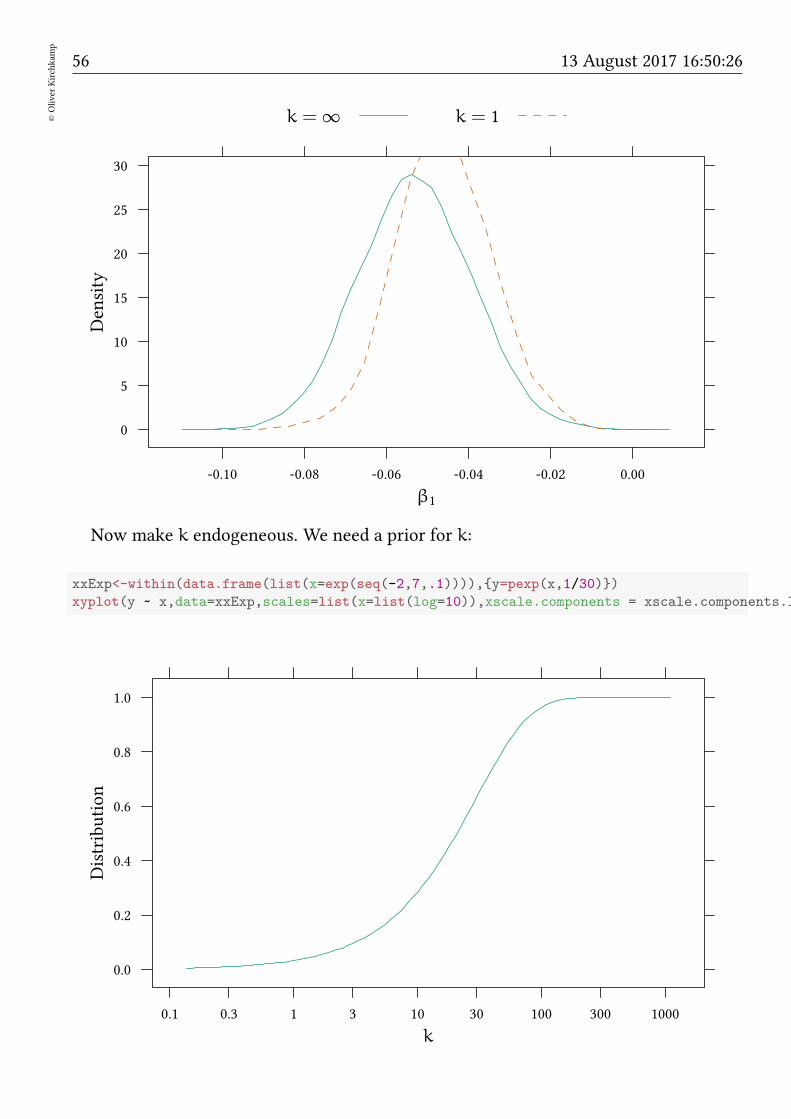
Now make k endogeneous. We need a prior for k:

xxExp<-within(data.frame(list(x=exp(seq(-2,7,.1)))),y=pexp(x,1/30))

xyplot(y ~ x,data=xxExp,scales=list(x=list(log=10)),xscale.components = xscale.components.log10.3,

k

Distribution

0.0

0.2

0.4

0.6

0.8

1.0

0.1 0.3 1 3 10 30 100 300 1000

Contents 57

©Oliver

Kirchkam

p

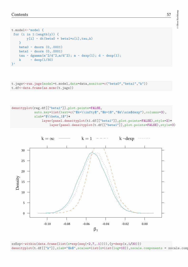
t.model<-’model


y[i] ~ dt(beta0 + beta1*x[i],tau,k)

beta0 ~ dnorm (0,.0001)

beta1 ~ dnorm (0,.0001)


k ~ dexp(1/30)

’

t.jags<-run.jags(model=t.model,data=data,monitor=c("beta0","beta1","k"))

t.df<-data.frame(as.mcmc(t.jags))

densityplot(reg.df[["beta1"]],plot.points=FALSE,

auto.key=list(text=c("$k=\\infty$","$k=1$","$k\\sim$dexp"),columns=3),

xlab="$\\beta_1$")+

layer(panel.densityplot(t1.df[["beta1"]],plot.points=FALSE),style=2)+

layer(panel.densityplot(t.df[["beta1"]],plot.points=FALSE),style=3)

β1

Density

0

5

10

15

20

25

30

-0.10 -0.08 -0.06 -0.04 -0.02 0.00

k = ∞ k = 1 k ∼dexp

xxExp<-within(data.frame(list(x=exp(seq(-2,7,.1)))),y=dexp(x,1/30))

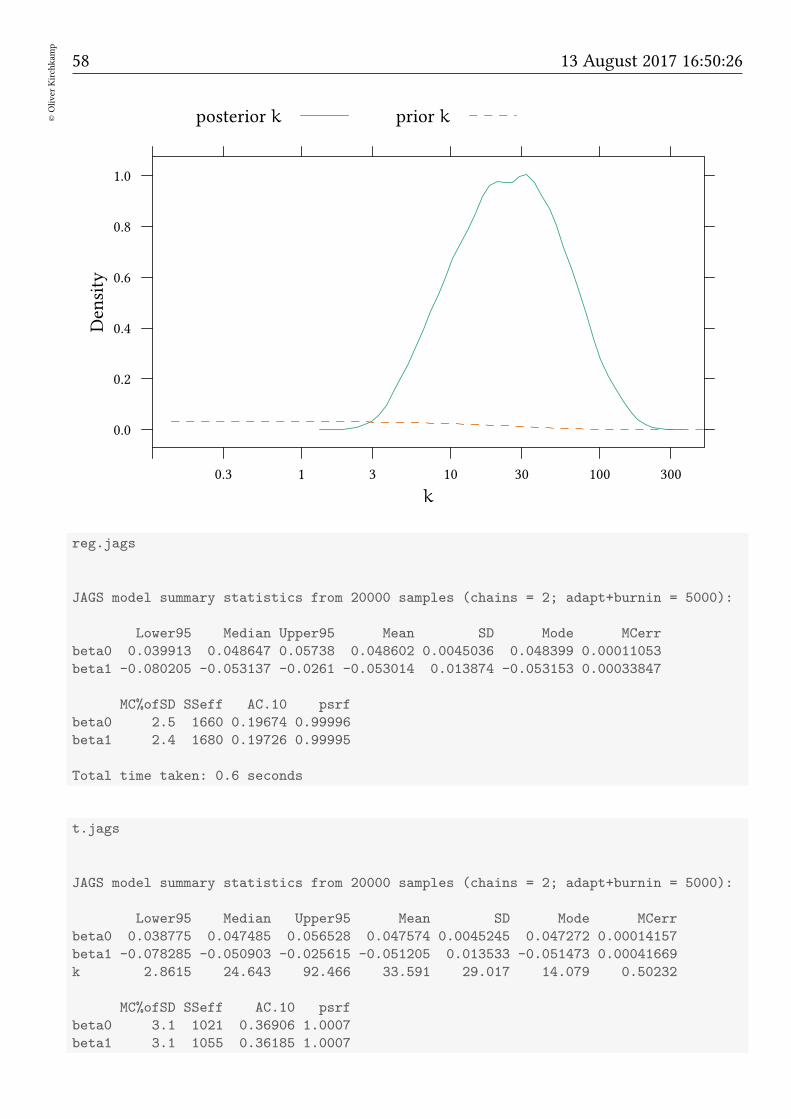
densityplot(t.df[["k"]],xlab="$k$",scales=list(x=list(log=10)),xscale.components = xscale.compo

58©Oliver

Kirchkam

p

13 August 2017 16:50:26

k

Density

0.0

0.2

0.4

0.6

0.8

1.0

0.3 1 3 10 30 100 300

posterior k prior k

reg.jags



beta0 0.039913 0.048647 0.05738 0.048602 0.0045036 0.048399 0.00011053

beta1 -0.080205 -0.053137 -0.0261 -0.053014 0.013874 -0.053153 0.00033847


beta0 2.5 1660 0.19674 0.99996

beta1 2.4 1680 0.19726 0.99995


t.jags



beta0 0.038775 0.047485 0.056528 0.047574 0.0045245 0.047272 0.00014157

beta1 -0.078285 -0.050903 -0.025615 -0.051205 0.013533 -0.051473 0.00041669

k 2.8615 24.643 92.466 33.591 29.017 14.079 0.50232


beta0 3.1 1021 0.36906 1.0007

beta1 3.1 1055 0.36185 1.0007

Contents 59

©Oliver

Kirchkam

p

k 1.7 3337 0.053228 1.0004


6.2 Robust regression with the Engel data

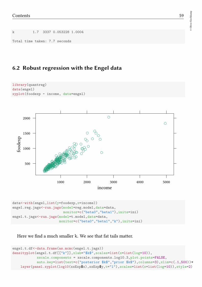
library(quantreg)

data(engel)

xyplot(foodexp ~ income, data=engel)

income

foodexp

500

1000

1500

2000

1000 2000 3000 4000 5000

data<-with(engel,list(y=foodexp,x=income))

engel.reg.jags<-run.jags(model=reg.model,data=data,

monitor=c("beta0","beta1"),inits=ini)

engel.t.jags<-run.jags(model=t.model,data=data,

monitor=c("beta0","beta1","k"),inits=ini)

Here we find a much smaller k. We see that fat tails matter.

engel.t.df<-data.frame(as.mcmc(engel.t.jags))

densityplot(engel.t.df[["k"]],xlab="$k$",scales=list(x=list(log=10)),

xscale.components = xscale.components.log10.3,plot.points=FALSE,

auto.key=list(text=c("posterior $k$","prior $k$"),columns=3),xlim=c(.1,500))+

layer(panel.xyplot(log10(xxExp$x),xxExp$y,t="l"),scales=list(x=list(log=10)),style=2)

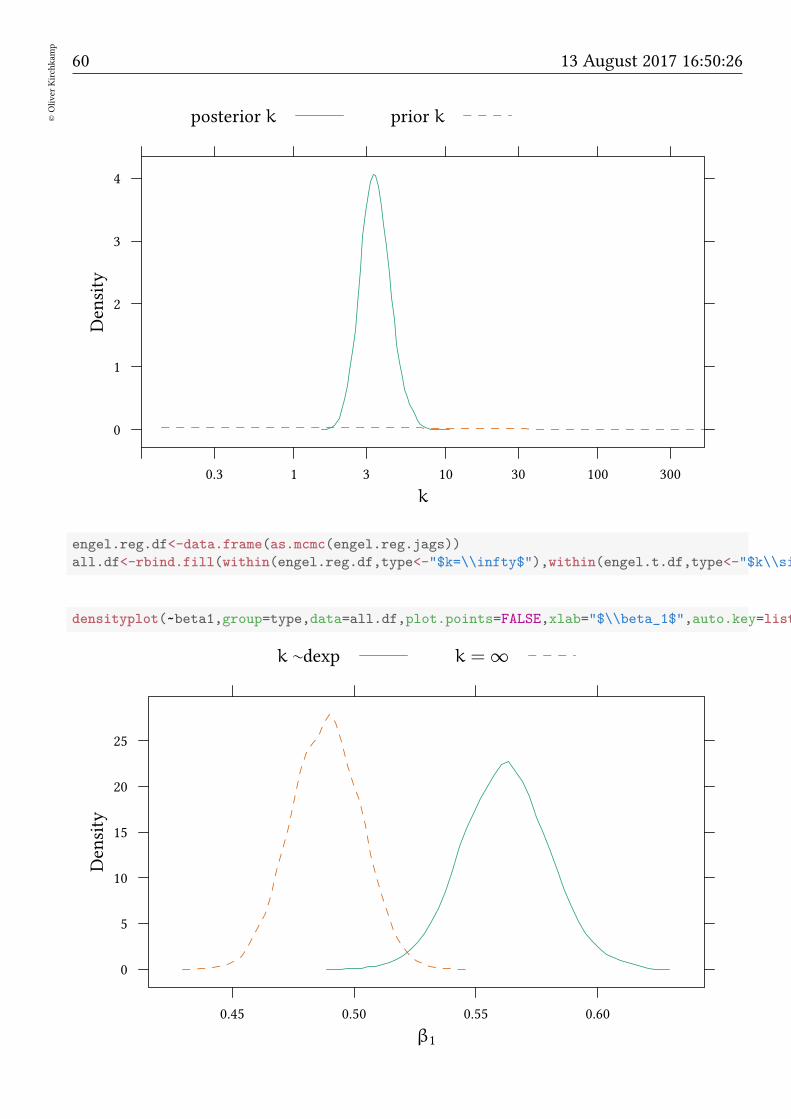
60©Oliver

Kirchkam

p

13 August 2017 16:50:26

k

Density

0

1

2

3

4

0.3 1 3 10 30 100 300

posterior k prior k

engel.reg.df<-data.frame(as.mcmc(engel.reg.jags))

all.df<-rbind.fill(within(engel.reg.df,type<-"$k=\\infty$"),within(engel.t.df,type<-"$k\\sim$dexp

densityplot(~beta1,group=type,data=all.df,plot.points=FALSE,xlab="$\\beta_1$",auto.key=list(

β1

Density

0

5

10

15

20

25

0.45 0.50 0.55 0.60

k ∼dexp k = ∞

Contents 61

©Oliver

Kirchkam

p

engel.reg.jags



beta0 112.5 143.34 174.37 143.37 15.917 143.64 0.32063 2 2465

beta1 0.45943 0.48864 0.51525 0.48848 0.014371 0.48796 0.00028645 2 2517

AC.10 psrf

beta0 0.072199 1.0003

beta1 0.069264 1.0004


engel.t.jags



beta0 49.531 79.555 110.84 79.526 15.465 80.325 0.52445 3.4 869

beta1 0.52548 0.56206 0.59697 0.5621 0.018052 0.5613 0.00060312 3.3 896

k 2.0817 3.4211 5.2599 3.5472 0.84881 3.2658 0.013462 1.6 3976

AC.10 psrf

beta0 0.41396 1.0005

beta1 0.41633 1.0006

k 0.053926 1.0001


6.3 Exercises

Consider the data set Wages from Ecdat. The data set contains seven observations foreach worker. Consider for each worker the first of these observations. You want to studythe impact of education on wage.

1. Could there be outliers in lwage?

2. How can you take outliers into account?

3. Estimate your model.

62©Oliver

Kirchkam

p

13 August 2017 16:50:26

7 Nonparametric

7.1 Preliminaries

• Is the “nonparametric” idea essentially frequentist?

• After all, with “nonparametrics” we avoid a discussion about distributions.

• Perhaps it would be more honest to model what we know about the distribution.

Still. . .

• Equivalent for “binomial test”: X ∼ dbern().

• Equivalent for “χ2 test”: X ∼ dpois().

Furthermore. . .

• As in the frequentist world we can translate one (less known) distribution to an-other by using ranks.

7.2 Example: Rank sum based comparison

Here we create two variables who both follow an exponential distribution. We mightforget this information and use ranks to compare.

set.seed(4)

xx<-rbind(data.frame(list(x=rexp(10,1),t=1)),

data.frame(list(x=rexp(20,3),t=2)))

wilcox.test(x~t,data=xx)

Wilcoxon rank sum test

data: x by t

W = 156, p-value = 0.01273

alternative hypothesis: true location shift is not equal to 0

densityplot(~x,group=t,data=xx)

Contents 63

©Oliver

Kirchkam

p

x

Density

0.0

0.5

1.0

1.5

0 1 2 3 4 5

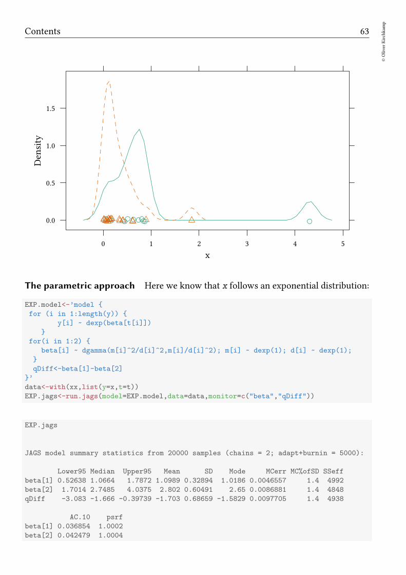
The parametric approach Here we know that x follows an exponential distribution:

EXP.model<-’model


y[i] ~ dexp(beta[t[i]])

for(i in 1:2)

beta[i] ~ dgamma(m[i]^2/d[i]^2,m[i]/d[i]^2); m[i] ~ dexp(1); d[i] ~ dexp(1);

qDiff<-beta[1]-beta[2]

’

data<-with(xx,list(y=x,t=t))

EXP.jags<-run.jags(model=EXP.model,data=data,monitor=c("beta","qDiff"))

EXP.jags



beta[1] 0.52638 1.0664 1.7872 1.0989 0.32894 1.0186 0.0046557 1.4 4992

beta[2] 1.7014 2.7485 4.0375 2.802 0.60491 2.65 0.0086881 1.4 4848

qDiff -3.083 -1.666 -0.39739 -1.703 0.68659 -1.5829 0.0097705 1.4 4938

AC.10 psrf

beta[1] 0.036854 1.0002

beta[2] 0.042479 1.0004

64©Oliver

Kirchkam

p

13 August 2017 16:50:26

qDiff 0.042407 0.99998


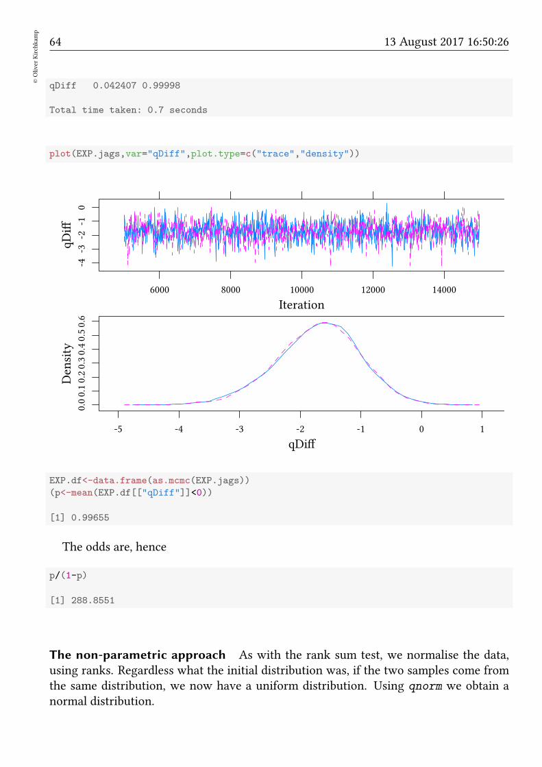
plot(EXP.jags,var="qDiff",plot.type=c("trace","density"))

Iteration

qDiff

-4-3

-2-1

0

6000 8000 10000 12000 14000

qDiff

Density

0.00.10.20.30.40.50.6

-5 -4 -3 -2 -1 0 1

EXP.df<-data.frame(as.mcmc(EXP.jags))

(p<-mean(EXP.df[["qDiff"]]<0))

[1] 0.99655

The odds are, hence

p/(1-p)

[1] 288.8551

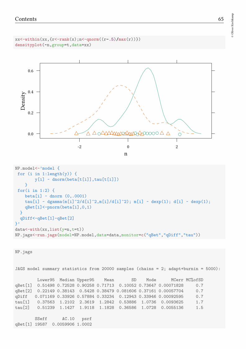
The non-parametric approach As with the rank sum test, we normalise the data,using ranks. Regardless what the initial distribution was, if the two samples come fromthe same distribution, we now have a uniform distribution. Using qnorm we obtain anormal distribution.

Contents 65

©Oliver

Kirchkam

p

xx<-within(xx,r<-rank(x);n<-qnorm((r-.5)/max(r)))

densityplot(~n,group=t,data=xx)

n

Density

0.0

0.2

0.4

0.6

-2 0 2

NP.model<-’model


y[i] ~ dnorm(beta[t[i]],tau[t[i]])

for(i in 1:2)

beta[i] ~ dnorm (0,.0001)

tau[i] ~ dgamma(m[i]^2/d[i]^2,m[i]/d[i]^2); m[i] ~ dexp(1); d[i] ~ dexp(1);

qBet[i]<-pnorm(beta[i],0,1)

qDiff<-qBet[1]-qBet[2]

’

data<-with(xx,list(y=n,t=t))

NP.jags<-run.jags(model=NP.model,data=data,monitor=c("qBet","qDiff","tau"))

NP.jags


Lower95 Median Upper95 Mean SD Mode MCerr MC%ofSD

qBet[1] 0.51498 0.72528 0.90258 0.71713 0.10052 0.73647 0.00071828 0.7

qBet[2] 0.22149 0.38143 0.5428 0.38479 0.081606 0.37161 0.00057704 0.7

qDiff 0.071169 0.33926 0.57884 0.33234 0.12943 0.33946 0.00092595 0.7

tau[1] 0.37563 1.2102 2.3619 1.2842 0.53886 1.0736 0.0093625 1.7

tau[2] 0.51239 1.1427 1.9118 1.1828 0.36586 1.0728 0.0055136 1.5

SSeff AC.10 psrf

qBet[1] 19587 0.0059906 1.0002

66©Oliver

Kirchkam

p

13 August 2017 16:50:26

qBet[2] 20000 -0.0088586 1.0002

qDiff 19539 -0.0039439 1.0002

tau[1] 3313 0.083678 1.0006

tau[2] 4403 0.045728 1.0006


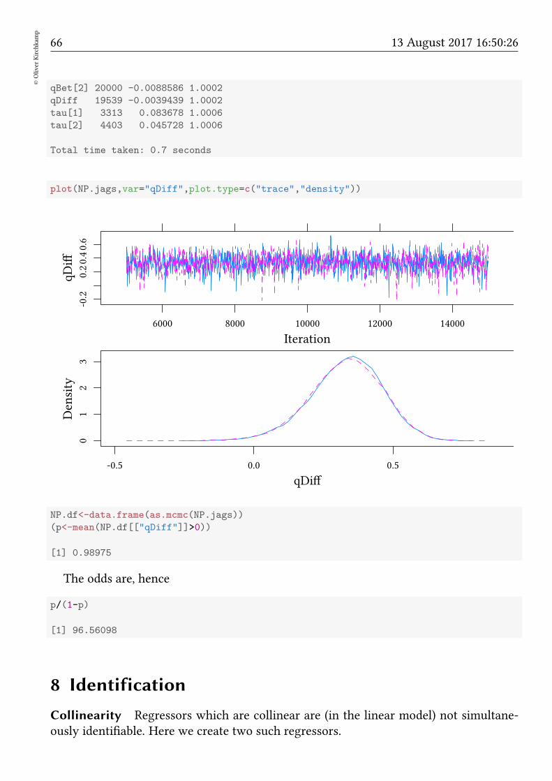
plot(NP.jags,var="qDiff",plot.type=c("trace","density"))

Iteration

qDiff

-0.2

0.20.40.6

6000 8000 10000 12000 14000

qDiff

Density

01

23

-0.5 0.0 0.5

NP.df<-data.frame(as.mcmc(NP.jags))

(p<-mean(NP.df[["qDiff"]]>0))

[1] 0.98975

The odds are, hence

p/(1-p)

[1] 96.56098

8 Identification

Collinearity Regressors which are collinear are (in the linear model) not simultane-ously identifiable. Here we create two such regressors.

Contents 67

©Oliver

Kirchkam

p

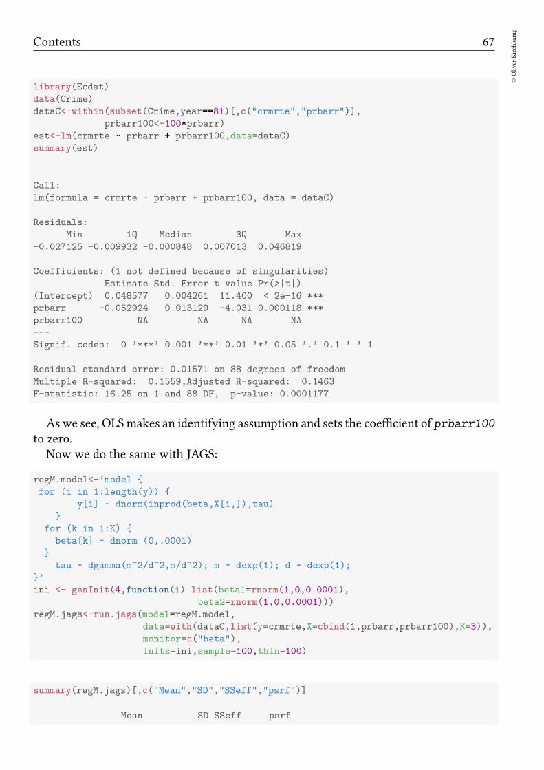
library(Ecdat)

data(Crime)

dataC<-within(subset(Crime,year==81)[,c("crmrte","prbarr")],

prbarr100<-100*prbarr)

est<-lm(crmrte ~ prbarr + prbarr100,data=dataC)

summary(est)

Call:

lm(formula = crmrte ~ prbarr + prbarr100, data = dataC)

Residuals:


-0.027125 -0.009932 -0.000848 0.007013 0.046819

Coefficients: (1 not defined because of singularities)


(Intercept) 0.048577 0.004261 11.400 < 2e-16 ***

prbarr -0.052924 0.013129 -4.031 0.000118 ***

prbarr100 NA NA NA NA

---

Signif. codes: 0 ’***’ 0.001 ’**’ 0.01 ’*’ 0.05 ’.’ 0.1 ’ ’ 1




Aswe see, OLSmakes an identifying assumption and sets the coefficient of prbarr100

to zero.Now we do the same with JAGS:

regM.model<-’model


y[i] ~ dnorm(inprod(beta,X[i,]),tau)

for (k in 1:K)

beta[k] ~ dnorm (0,.0001)


’

ini <- genInit(4,function(i) list(beta1=rnorm(1,0,0.0001),

beta2=rnorm(1,0,0.0001)))

regM.jags<-run.jags(model=regM.model,

data=with(dataC,list(y=crmrte,X=cbind(1,prbarr,prbarr100),K=3)),

monitor=c("beta"),

inits=ini,sample=100,thin=100)

summary(regM.jags)[,c("Mean","SD","SSeff","psrf")]

Mean SD SSeff psrf

68©Oliver

Kirchkam

p

13 August 2017 16:50:26

beta[1] 0.048510672 0.004424766 463 1.003878

beta[2] 0.390078051 1.539589057 9 6.558625

beta[3] -0.004426064 0.015395795 9 6.564672

• Standard errors for coefficients are much larger.

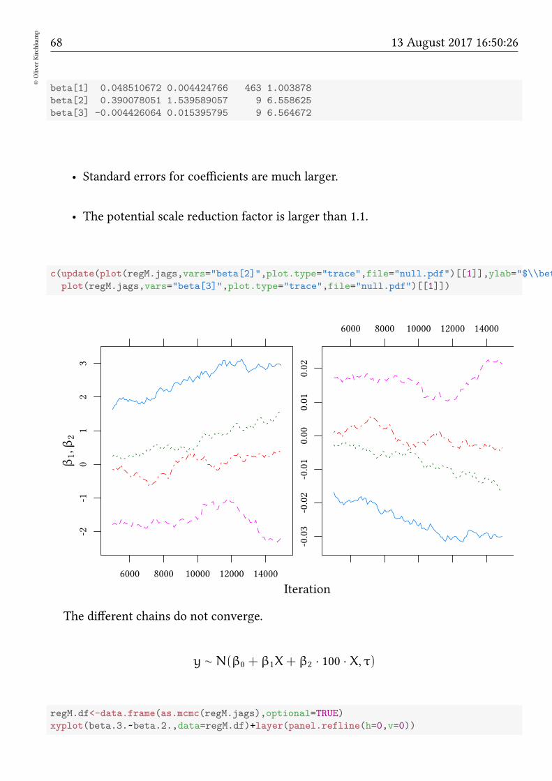
• The potential scale reduction factor is larger than 1.1.

c(update(plot(regM.jags,vars="beta[2]",plot.type="trace",file="null.pdf")[[1]],ylab="$\\beta_1,\\beta_2

plot(regM.jags,vars="beta[3]",plot.type="trace",file="null.pdf")[[1]])

Iteration

β1,β

2

-2-1

01

23

6000 8000 10000 12000 14000

6000 8000 10000 12000 14000

-0.03

-0.02

-0.01

0.00

0.01

0.02

The different chains do not converge.

y ∼ N(β0 + β1X+ β2 · 100 · X, τ)

regM.df<-data.frame(as.mcmc(regM.jags),optional=TRUE)

xyplot(beta.3.~beta.2.,data=regM.df)+layer(panel.refline(h=0,v=0))

Contents 69

©Oliver

Kirchkam

p

beta.2.

beta.3.

-0.03

-0.02

-0.01

0.00

0.01

0.02

-2 -1 0 1 2 3

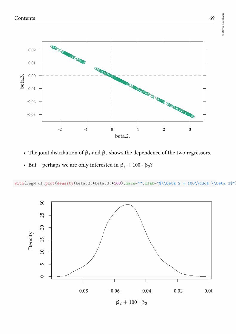
• The joint distribution of β1 and β2 shows the dependence of the two regressors.

• But – perhaps we are only interested in β2 + 100 · β3?

with(regM.df,plot(density(beta.2.+beta.3.*100),main="",xlab="$\\beta_2 + 100\\cdot \\beta_3$"))

-0.08 -0.06 -0.04 -0.02 0.00

05

1015

2025

30

β2 + 100 · β3

Density

70©Oliver

Kirchkam

p

13 August 2017 16:50:26

Identification Summary

• Many frequentist tools try to obtain point estimates. Hence, they must detectunder-identification. Often they make identifying assumptions on their own.

• In the Bayesian world we estimate a joint distribution. Under-identification neednot be a problem. It shows up as large standard deviation, lack of convergence, alarge gelman.diag, etc.

9 Discrete Choice

9.1 Labor force participation

library(Ecdat)

data(Participation)

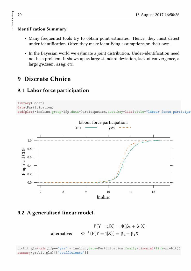
ecdfplot(~lnnlinc,group=lfp,data=Participation,auto.key=list(title="labour force participation:"

lnnlinc

EmpiricalCDF

0.0

0.2

0.4

0.6

0.8

1.0

7 8 9 10 11 12

labour force participation:no yes

9.2 A generalised linear model

P(Y = 1|X) = Φ(β0 + β1X)

alternative: Φ−1 (P(Y = 1|X)) = β0 + β1X

probit.glm<-glm(lfp=="yes" ~ lnnlinc,data=Participation,family=binomial(link=probit))

summary(probit.glm)[["coefficients"]]

Contents 71

©Oliver

Kirchkam

p

Estimate Std. Error z value Pr(>|z|)

(Intercept) 5.9705580 1.1943613 4.998955 0.0000005764194

lnnlinc -0.5685645 0.1117688 -5.086972 0.0000003638259

9.3 Bayesian discrete choice

probit.model <- ’model


y[i] ~ dbern(p[i])

p[i] <- phi(inprod(X[i,],beta))

for (k in 1:K)


’

Part.data<-with(Participation,list(y=as.numeric(lfp=="yes"),X=cbind(1,lnnlinc),K=2))

probit.jags<-run.jags(model=probit.model,modules="glm",

data=Part.data,inits=ini,monitor=c("beta"))

summary(probit.jags)[,c("Mean","SD","SSeff","psrf")]

Mean SD SSeff psrf

beta[1] 5.9838734 1.1902539 29769 1.000072

beta[2] -0.5698306 0.1114429 29693 1.000070

(We should use phi(...) and not pnorm(...,0,1). The latter is slower to converge.)

The following specification is equivalent:

probit.model <- ’model


y[i] ~ dbern(p[i])

probit(p[i]) <- inprod(X[i,],beta)

for (k in 1:K)


’

Part.data<-with(Participation,list(y=as.numeric(lfp=="yes"),X=cbind(1,lnnlinc),K=2))

probit.jags<-run.jags(model=probit.model,modules="glm",

data=Part.data,inits=ini,monitor=c("beta"))

summary(probit.jags)[,c("Mean","SD","SSeff","psrf")]

Mean SD SSeff psrf

beta[1] 5.9838734 1.1902539 29769 1.000072

beta[2] -0.5698306 0.1114429 29693 1.000070

72©Oliver

Kirchkam

p

13 August 2017 16:50:26

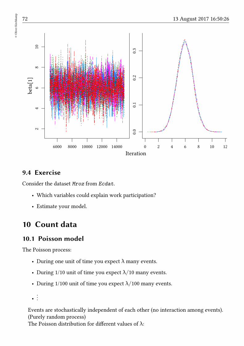
Iteration

beta[1]

24

68

10

6000 8000 10000 12000 14000

0.0

0.1

0.2

0.3

0 2 4 6 8 10 12

9.4 Exercise

Consider the dataset Mroz from Ecdat.

• Which variables could explain work participation?

• Estimate your model.

10 Count data

10.1 Poisson model

The Poisson process:

• During one unit of time you expect λ many events.

• During 1/10 unit of time you expect λ/10 many events.

• During 1/100 unit of time you expect λ/100 many events.

•...

Events are stochastically independent of each other (no interaction among events).(Purely random process)The Poisson distribution for different values of λ:

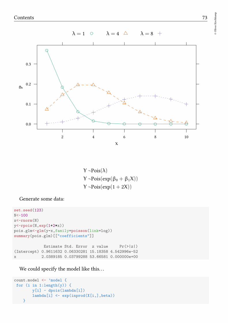
Contents 73

©Oliver

Kirchkam

p

x

P

0.0

0.1

0.2

0.3

2 4 6 8 10

λ = 1 λ = 4 λ = 8

Y ∼Pois(λ)

Y ∼Pois(exp(β0 + β1X))

Y ∼Pois(exp(1+ 2X))

Generate some data:

set.seed(123)

N<-100

x<-rnorm(N)

y<-rpois(N,exp(1+2*x))

pois.glm<-glm(y~x,family=poisson(link=log))

summary(pois.glm)[["coefficients"]]

Estimate Std. Error z value Pr(>|z|)

(Intercept) 0.9611632 0.06330281 15.18358 4.542996e-52

x 2.0389185 0.03799288 53.66581 0.000000e+00

We could specify the model like this. . .

count.model <- ’model


y[i] ~ dpois(lambda[i])

lambda[i] <- exp(inprod(X[i,],beta))

74©Oliver

Kirchkam

p

13 August 2017 16:50:26

for (k in 1:K)


’

count.jags<-run.jags(model=count.model,modules="glm",

data=list(y=y,X=cbind(1,x),K=2),inits=ini,monitor=c("beta"))

summary(count.jags)[,c("Mean","SD","SSeff","psrf")]

Mean SD SSeff psrf

beta[1] 0.9583643 0.06270963 3032 1.000460

beta[2] 2.0400627 0.03769276 3648 1.000473

. . . or like this. . .

count.model <- ’model


y[i] ~ dpois(lambda[i])

log(lambda[i]) <- inprod(X[i,],beta)

for (k in 1:K)


’

count.jags<-run.jags(model=count.model,modules="glm",

data=list(y=y,X=cbind(1,x),K=2),inits=ini,monitor=c("beta"))

summary(count.jags)[,c("Mean","SD","SSeff","psrf")]

Mean SD SSeff psrf

beta[1] 0.9583643 0.06270963 3032 1.000460

beta[2] 2.0400627 0.03769276 3648 1.000473

10.2 Negative binomial

Count data and the negative binomial distribution

Poisson distribution: Pois(λ)

Mean: λ

Variance: λ

Negative binomial distribution: NB(µ, r)

Mean: µ

Variance: µ+ µ2/r

Poisson is a special case of NB:

limr→∞

NB(µ, r) = Pois(µ)

The NB distribution for µ = 4 and for different values of r:

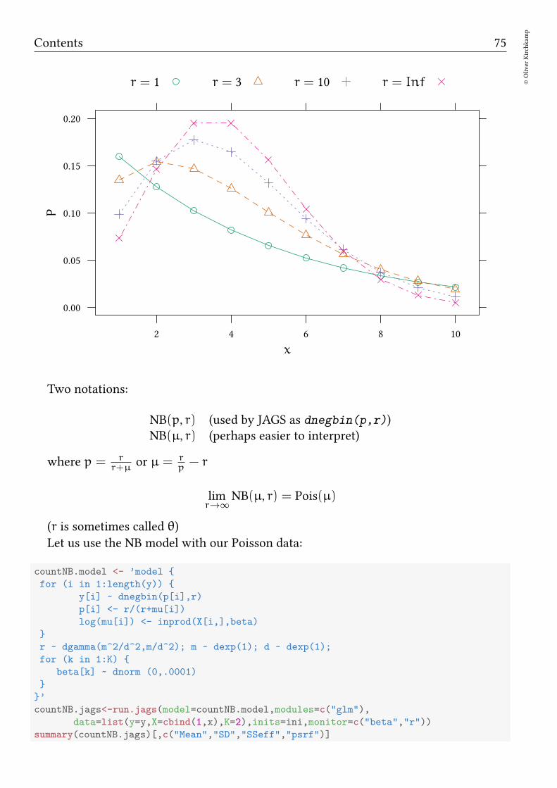
Contents 75

©Oliver

Kirchkam

p

x

P

0.00

0.05

0.10

0.15

0.20

2 4 6 8 10

r = 1 r = 3 r = 10 r = Inf

Two notations:

NB(p, r) (used by JAGS as dnegbin(p,r))NB(µ, r) (perhaps easier to interpret)

where p = rr+µ

or µ = rp− r

limr→∞

NB(µ, r) = Pois(µ)

(r is sometimes called θ)

Let us use the NB model with our Poisson data:

countNB.model <- ’model


y[i] ~ dnegbin(p[i],r)

p[i] <- r/(r+mu[i])

log(mu[i]) <- inprod(X[i,],beta)

r ~ dgamma(m^2/d^2,m/d^2); m ~ dexp(1); d ~ dexp(1);

for (k in 1:K)


’

countNB.jags<-run.jags(model=countNB.model,modules=c("glm"),

data=list(y=y,X=cbind(1,x),K=2),inits=ini,monitor=c("beta","r"))

summary(countNB.jags)[,c("Mean","SD","SSeff","psrf")]

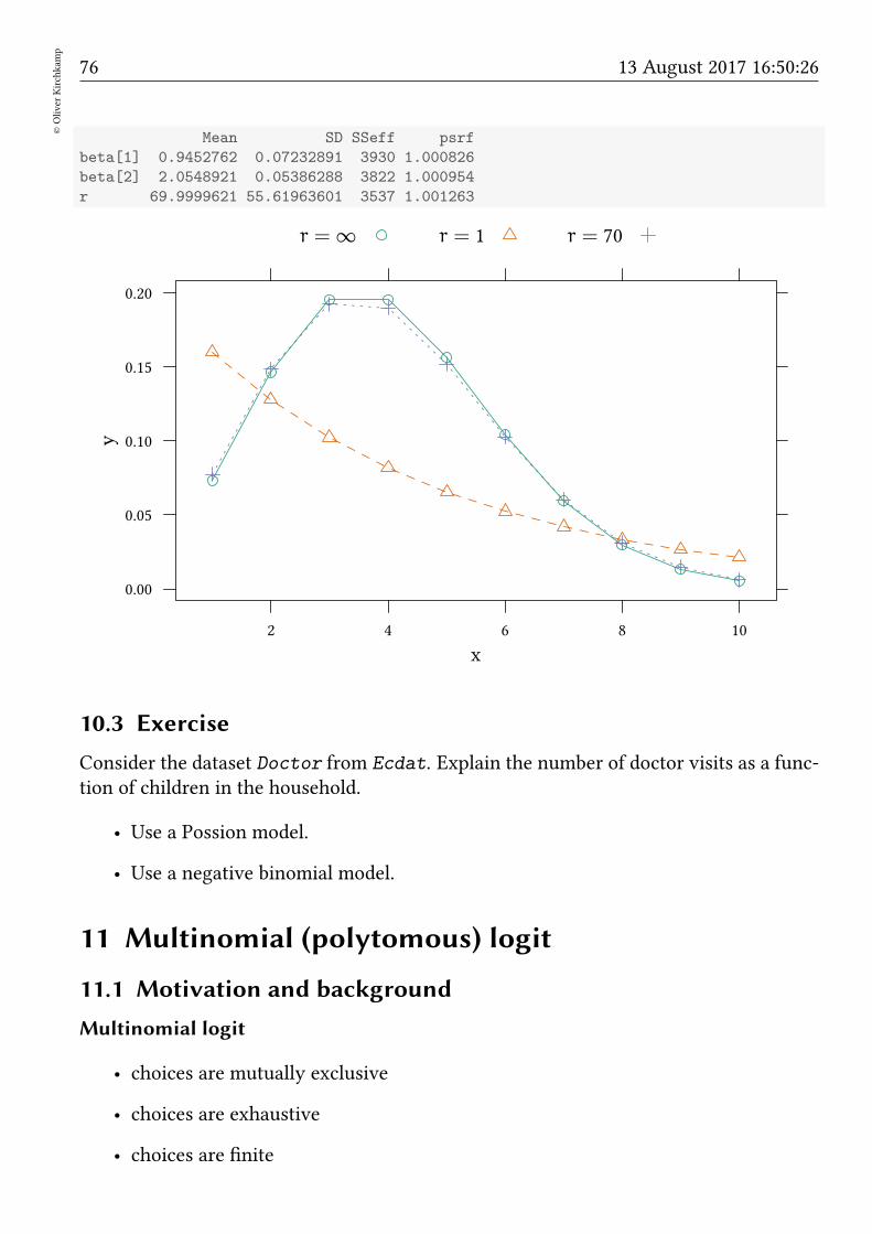
76©Oliver

Kirchkam

p

13 August 2017 16:50:26

Mean SD SSeff psrf

beta[1] 0.9452762 0.07232891 3930 1.000826

beta[2] 2.0548921 0.05386288 3822 1.000954

r 69.9999621 55.61963601 3537 1.001263

x

y

0.00

0.05

0.10

0.15

0.20

2 4 6 8 10

r = ∞ r = 1 r = 70

10.3 Exercise

Consider the dataset Doctor from Ecdat. Explain the number of doctor visits as a func-tion of children in the household.

• Use a Possion model.

• Use a negative binomial model.

11 Multinomial (polytomous) logit

11.1 Motivation and background

Multinomial logit

• choices are mutually exclusive

• choices are exhaustive

• choices are finite

Contents 77

©Oliver

Kirchkam

p

Problems

• one can map problems that do not look mutually exclusive or not exhaustive intoa problem that is

E.g.: heating modes: gas / oil / wood / electricity

What about households which use, e.g., gas + electricity→

– introduce an additional category

– ask for ‘primary source of heating’

Some households do not use any of the above:

– introduce an additional category

• Using discrete choice models for metric variables

– E.g.: consumption of goods which follow a non-linear tariff (telephone, elec-tricity)

Random utility models

Can we tell a story like in the logit/probit case?

A latent variable model (random utility model):

η1 = x ′β1 + ξ1

η2 = x ′β2 + ξ2

η3 = x ′β3 + ξ3...

The decision maker chooses alternative k if ηk > ηj for all j

Note: these models are equivalent to their affine transformations.

Normalisations

• We often normalise the constant part of one of the equations to zero.

• If ξj are i.i.d. we often normalise their variance to a convenient value.

(this implies that different distributions for ξ will lead to different scales for coef-ficients — logit coefficients will be π/

√6 times larger than probit.)

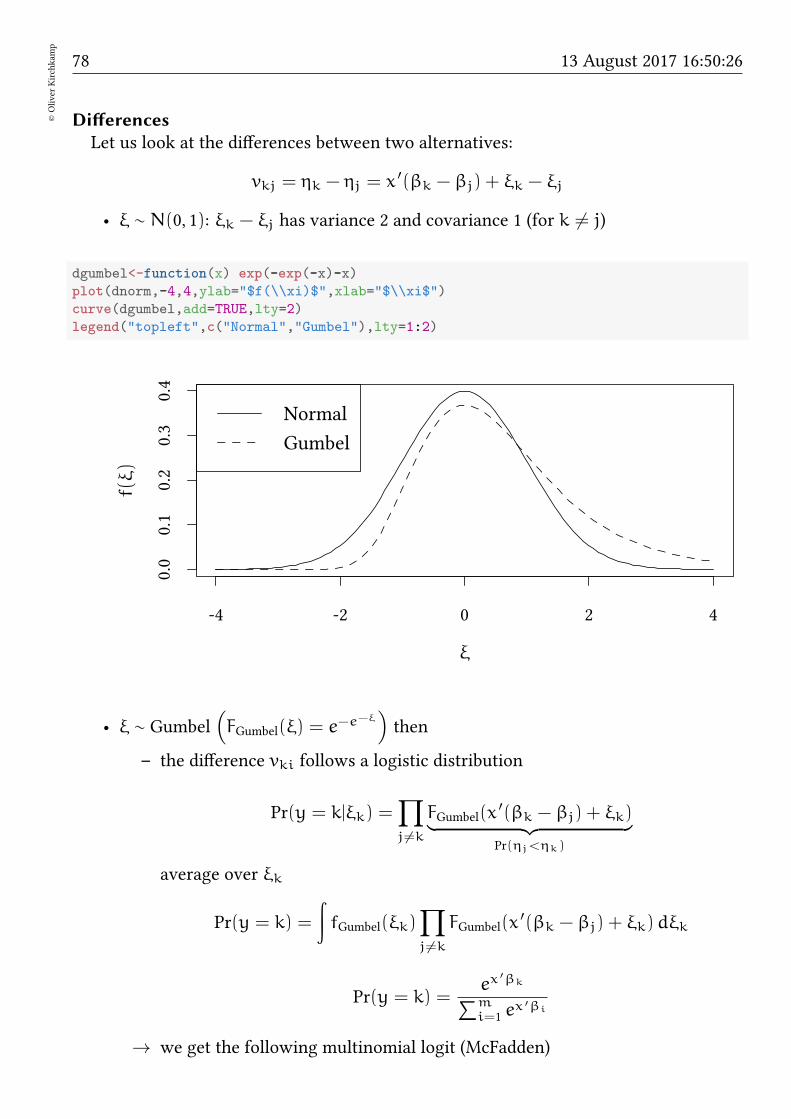
78©Oliver

Kirchkam

p

13 August 2017 16:50:26

Differences

Let us look at the differences between two alternatives:

vkj = ηk − ηj = x′(βk − βj) + ξk − ξj

• ξ ∼ N(0, 1): ξk − ξj has variance 2 and covariance 1 (for k 6= j)

dgumbel<-function(x) exp(-exp(-x)-x)

plot(dnorm,-4,4,ylab="$f(\\xi)$",xlab="$\\xi$")

curve(dgumbel,add=TRUE,lty=2)

legend("topleft",c("Normal","Gumbel"),lty=1:2)

-4 -2 0 2 4

0.0

0.1

0.2

0.3

0.4

ξ

f(ξ)

Normal

Gumbel

• ξ ∼ Gumbel(

FGumbel(ξ) = e−e−ξ

)

then

– the difference vki follows a logistic distribution

Pr(y = k|ξk) =∏

j 6=k

FGumbel(x′(βk − βj) + ξk)

︸︷︷︸Pr(ηj<ηk)

average over ξk

Pr(y = k) =

∫

fGumbel(ξk)∏

j 6=k

FGumbel(x′(βk − βj) + ξk)dξk

Pr(y = k) =ex

′βk

∑mi=1 e

x′βi

→ we get the following multinomial logit (McFadden)

Contents 79

©Oliver

Kirchkam

p

Pr(y = 1) =ex

′β1

∑mk=1 e

x′βk

Pr(y = 2) =ex

′β2

∑mk=1 e

x′βk

Pr(y = 3) =ex

′β3

∑mk=1 e

x′βk

...

• 0 < Pr(y = k) < 1

•∑

k Pr(y = k) = 1

↑ βk are not identified

Normalise:

Pr(y = 1) =1

1+∑m

k=2 ex′βk

Pr(y = 2) =ex

′β2

1+∑m

k=2 ex′βk

Pr(y = 3) =ex

′β3

1+∑m

k=2 ex′βk

...

the odds ratios are:Pr(y = k)

Pr(y = 1)= ex

′βk

This is a strong assumption on the error terms.

Indenpendence from irrelevant alternatives — IIA

Example:

• Dependent = choice of travel mode

• unobservable = personal preference for/againstmeans ofmass transportation (tube/train).

Pr(y=tube)Pr(y=1)

= ex′βtube Pr(y=train)

Pr(y=1)= ex

′βtrain

80©Oliver

Kirchkam

p

13 August 2017 16:50:26

• → choices/error terms are correlated.

→ multinomial logit can represent systematic variation of choices (explained by ob-served characteristics) but not systematic individual (unobserved) variation of choices.

The log-likelihood:

With Ik(yi) =

1 if yi = i

0 otherwise

logL =∑

i

m∑

k=1

Ik(yi) log Pr(yi = k)

=∑

i

m∑

k=1

Ik(yi) logex

′

iβk

1+∑m

k=2 ex′

iβk

this function logL is globally concave in β (McFadden, 1974)

11.2 Example

The purpose of this example is to illustrate an identification problem in the context ofmultinomial logit. There are different ways to describe the same choices. In the examplewe see that we use one set of parameters (mat) to generate the choices but the estimatorgives us a different set of parameters back (coef(est)). We also see how these two setsof parameters are related.

Let us first create individual explanatory variables, x1, x2.

N<-100

sd<-10

ex <- cbind(x1=runif(N),x2=runif(N))

head(ex)

x1 x2

[1,] 0.2875775 0.5999890

[2,] 0.7883051 0.3328235

[3,] 0.4089769 0.4886130

[4,] 0.8830174 0.9544738

[5,] 0.9404673 0.4829024

[6,] 0.0455565 0.8903502

The following matrix determines how individual characteristics translate into prefer-ences for three choices:

mat<-rbind(c(400,0),

c(250,200),

c(100,300))

mat

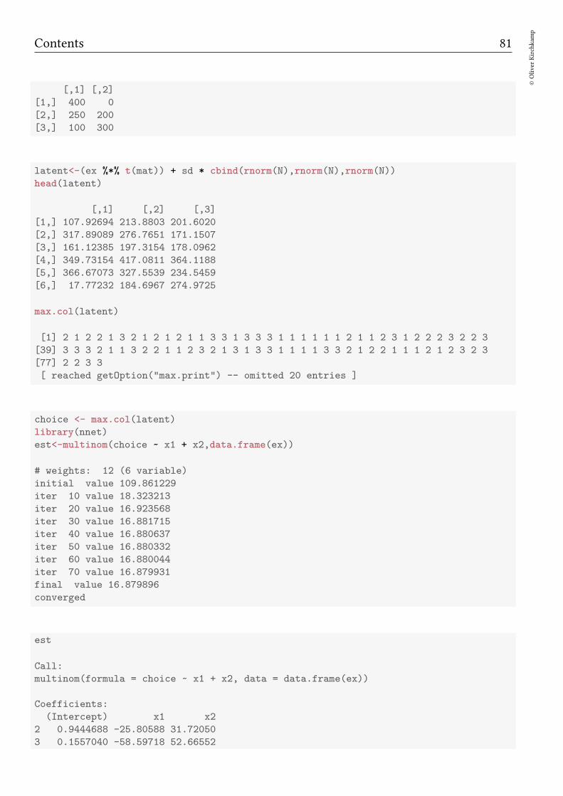
Contents 81

©Oliver

Kirchkam

p

[,1] [,2]

[1,] 400 0

[2,] 250 200

[3,] 100 300

latent<-(ex %*% t(mat)) + sd * cbind(rnorm(N),rnorm(N),rnorm(N))

head(latent)

[,1] [,2] [,3]

[1,] 107.92694 213.8803 201.6020

[2,] 317.89089 276.7651 171.1507

[3,] 161.12385 197.3154 178.0962

[4,] 349.73154 417.0811 364.1188

[5,] 366.67073 327.5539 234.5459

[6,] 17.77232 184.6967 274.9725

max.col(latent)

[1] 2 1 2 2 1 3 2 1 2 1 2 1 1 3 3 1 3 3 3 1 1 1 1 1 1 2 1 1 2 3 1 2 2 2 3 2 2 3

[39] 3 3 3 2 1 1 3 2 2 1 1 2 3 2 1 3 1 3 3 1 1 1 1 3 3 2 1 2 2 1 1 1 2 1 2 3 2 3

[77] 2 2 3 3

[ reached getOption("max.print") -- omitted 20 entries ]

choice <- max.col(latent)

library(nnet)

est<-multinom(choice ~ x1 + x2,data.frame(ex))

# weights: 12 (6 variable)

initial value 109.861229

iter 10 value 18.323213

iter 20 value 16.923568

iter 30 value 16.881715

iter 40 value 16.880637

iter 50 value 16.880332

iter 60 value 16.880044

iter 70 value 16.879931

final value 16.879896

converged

est

Call:

multinom(formula = choice ~ x1 + x2, data = data.frame(ex))

Coefficients:

(Intercept) x1 x2

2 0.9444688 -25.80588 31.72050

3 0.1557040 -58.59718 52.66552

82©Oliver

Kirchkam

p

13 August 2017 16:50:26

Residual Deviance: 33.75979

AIC: 45.75979

Note that the estimated coefficients are not the matrix of coefficients mat that we em-ployed above. However, they are a projection. We are expecting this:

mat

[,1] [,2]

[1,] 400 0

[2,] 250 200

[3,] 100 300

but we got that:

coef(est)

(Intercept) x1 x2

2 0.9444688 -25.80588 31.72050

3 0.1557040 -58.59718 52.66552

The estimator normalises the first category to zero

mat

[,1] [,2]

[1,] 400 0

[2,] 250 200

[3,] 100 300

mat - cbind(c(1,1,1)) %*% mat[1,]

[,1] [,2]

[1,] 0 0

[2,] -150 200

[3,] -300 300

and sets the variance to one:

(mat - cbind(c(1,1,1)) %*% mat[1,])*pi / sqrt(6) / 10

[,1] [,2]

[1,] 0.00000 0.00000

[2,] -19.23825 25.65100

[3,] -38.47649 38.47649

To access estimation results we have the usual extractor functions:

coef(est)

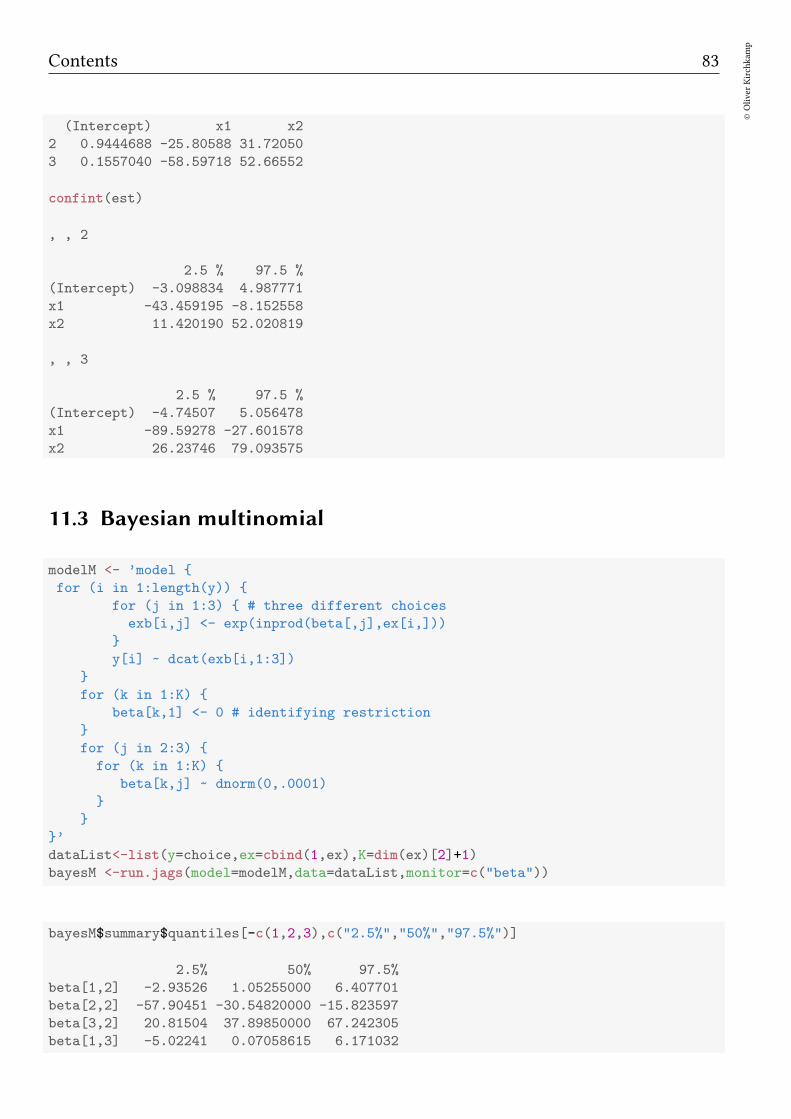
Contents 83

©Oliver

Kirchkam

p

(Intercept) x1 x2

2 0.9444688 -25.80588 31.72050

3 0.1557040 -58.59718 52.66552

confint(est)

, , 2

2.5 % 97.5 %

(Intercept) -3.098834 4.987771

x1 -43.459195 -8.152558

x2 11.420190 52.020819

, , 3

2.5 % 97.5 %

(Intercept) -4.74507 5.056478

x1 -89.59278 -27.601578

x2 26.23746 79.093575

11.3 Bayesian multinomial

modelM <- ’model


for (j in 1:3) # three different choices

exb[i,j] <- exp(inprod(beta[,j],ex[i,]))

y[i] ~ dcat(exb[i,1:3])

for (k in 1:K)

beta[k,1] <- 0 # identifying restriction

for (j in 2:3)

for (k in 1:K)

beta[k,j] ~ dnorm(0,.0001)

’

dataList<-list(y=choice,ex=cbind(1,ex),K=dim(ex)[2]+1)

bayesM <-run.jags(model=modelM,data=dataList,monitor=c("beta"))

bayesM$summary$quantiles[-c(1,2,3),c("2.5%","50%","97.5%")]

2.5% 50% 97.5%

beta[1,2] -2.93526 1.05255000 6.407701

beta[2,2] -57.90451 -30.54820000 -15.823597

beta[3,2] 20.81504 37.89850000 67.242305

beta[1,3] -5.02241 0.07058615 6.171032

84©Oliver

Kirchkam

p

13 August 2017 16:50:26

beta[2,3] -109.86352 -71.58410000 -44.914368

beta[3,3] 41.19685 64.41970000 95.933505

confint(est)

, , 2

2.5 % 97.5 %

(Intercept) -3.098834 4.987771

x1 -43.459195 -8.152558

x2 11.420190 52.020819

, , 3

2.5 % 97.5 %

(Intercept) -4.74507 5.056478

x1 -89.59278 -27.601578

x2 26.23746 79.093575

11.4 Exercise

Consider the data set ModeChoice from Ecdat.

• Which variables could explain the transport mode?


12 Ordered probit

12.1 Model

We observe whether latent variables x ′β are in an interval

Pr(yi = 1) = Pr(κ0 < x′iβ+ u 6 κ1)

Pr(yi = 2) = Pr(κ1 < x′iβ+ u 6 κ2)

Pr(yi = 3) = Pr(κ2 < x′iβ+ u 6 κ3)

...

or (solving for u)

Pr(yi = 1) = Pr(κ0 − x′iβ < u 6 κ1 − x

′iβ)

Pr(yi = 2) = Pr(κ1 − x′iβ < u 6 κ2 − x

′iβ)

Pr(yi = 3) = Pr(κ2 − x′iβ < u 6 κ3 − x

′iβ)

...

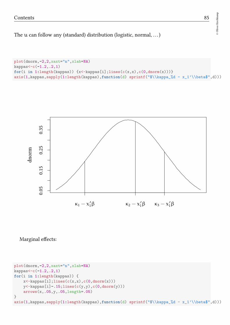
Contents 85

©Oliver

Kirchkam

p

The u can follow any (standard) distribution (logistic, normal, . . . )

plot(dnorm,-2,2,xaxt="n",xlab=NA)

kappas<-c(-1.2,.2,1)

for(i in 1:length(kappas)) x<-kappas[i];lines(c(x,x),c(0,dnorm(x)))

axis(1,kappas,sapply(1:length(kappas),function(d) sprintf("$\\kappa_%d - x_1’\\beta$",d)))

0.05

0.15

0.25

0.35

dnorm

κ1 − x′1β κ2 − x

′1β κ3 − x

′1β

Marginal effects:

plot(dnorm,-2,2,xaxt="n",xlab=NA)

kappas<-c(-1.2,.2,1)

for(i in 1:length(kappas))

x<-kappas[i];lines(c(x,x),c(0,dnorm(x)))

y<-kappas[i]-.15;lines(c(y,y),c(0,dnorm(y)))

arrows(x,.05,y,.05,length=.05)

axis(1,kappas,sapply(1:length(kappas),function(d) sprintf("$\\kappa_%d - x_1’\\beta$",d)))

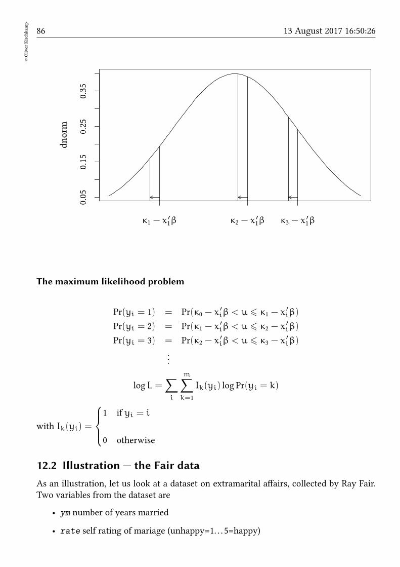
86©Oliver

Kirchkam

p

13 August 2017 16:50:26

0.05

0.15

0.25

0.35

dnorm

κ1 − x′1β κ2 − x

′1β κ3 − x

′1β

The maximum likelihood problem

Pr(yi = 1) = Pr(κ0 − x′iβ < u 6 κ1 − x

′iβ)

Pr(yi = 2) = Pr(κ1 − x′iβ < u 6 κ2 − x

′iβ)

Pr(yi = 3) = Pr(κ2 − x′iβ < u 6 κ3 − x

′iβ)

...

logL =∑

i

m∑

k=1

Ik(yi) log Pr(yi = k)

with Ik(yi) =

1 if yi = i

0 otherwise

12.2 Illustration — the Fair data

As an illustration, let us look at a dataset on extramarital affairs, collected by Ray Fair.Two variables from the dataset are

• ym number of years married

• rate self rating of mariage (unhappy=1. . . 5=happy)

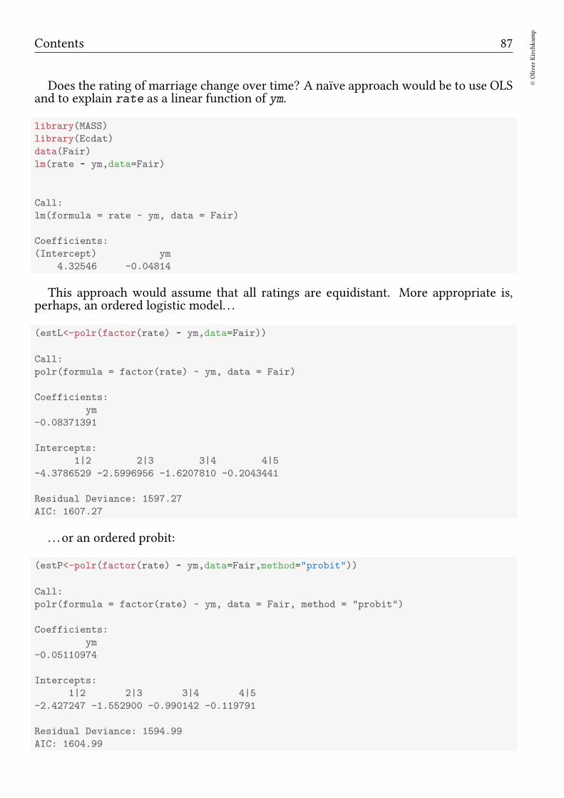
Contents 87

©Oliver

Kirchkam

p

Does the rating of marriage change over time? A naïve approach would be to use OLSand to explain rate as a linear function of ym.

library(MASS)

library(Ecdat)

data(Fair)

lm(rate ~ ym,data=Fair)

Call:

lm(formula = rate ~ ym, data = Fair)

Coefficients:

(Intercept) ym

4.32546 -0.04814

This approach would assume that all ratings are equidistant. More appropriate is,perhaps, an ordered logistic model. . .

(estL<-polr(factor(rate) ~ ym,data=Fair))

Call:

polr(formula = factor(rate) ~ ym, data = Fair)

Coefficients:

ym

-0.08371391

Intercepts:

1|2 2|3 3|4 4|5

-4.3786529 -2.5996956 -1.6207810 -0.2043441


AIC: 1607.27

. . . or an ordered probit:

(estP<-polr(factor(rate) ~ ym,data=Fair,method="probit"))

Call:

polr(formula = factor(rate) ~ ym, data = Fair, method = "probit")

Coefficients:

ym

-0.05110974

Intercepts:

1|2 2|3 3|4 4|5

-2.427247 -1.552900 -0.990142 -0.119791


AIC: 1604.99

88©Oliver

Kirchkam

p

13 August 2017 16:50:26

The following graph illustrates the estimated thresholds κi:

probFig <- function (est,main)

plot(function(x) x * est$coef,0,55,ylab="$\\kappa$",xlab="years of marriage",main=main)

for (a in est$zeta)

abline(h=a)

lab=names(est$zeta)[which(est$zeta==a)]

text(1,a,labels=lab,adj=c(0,1))

probFig(estL,main="ordered logistic")

probFig(estP,main="ordered probit")

0 10 20 30 40 50

-4-3

-2-1

0

ordered logistic

years of marriage

κ

1—2

2—3

3—4

4—5

0 10 20 30 40 50

-2.5

-1.5

-0.5

ordered probit

years of marriage

κ

1—2

2—3

3—4

4—5

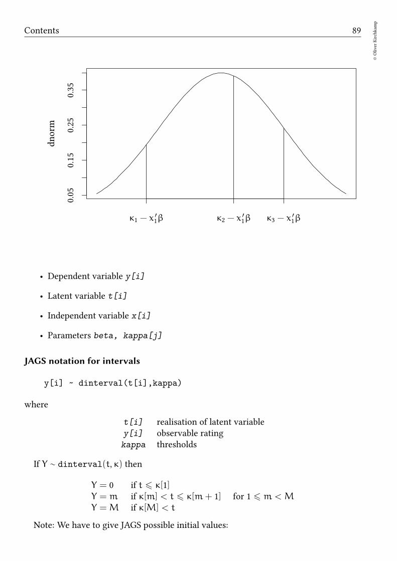
Contents 89

©Oliver

Kirchkam

p

0.05

0.15

0.25

0.35

dnorm

κ1 − x′1β κ2 − x

′1β κ3 − x

′1β

• Dependent variable y[i]

• Latent variable t[i]

• Independent variable x[i]

• Parameters beta, kappa[j]

JAGS notation for intervals

y[i] ~ dinterval(t[i],kappa)

where

t[i] realisation of latent variabley[i] observable ratingkappa thresholds

If Y ∼ dinterval(t, κ) then

Y = 0 if t 6 κ[1]Y = m if κ[m] < t 6 κ[m+ 1] for 1 6 m <M

Y =M if κ[M] < t

Note: We have to give JAGS possible initial values:

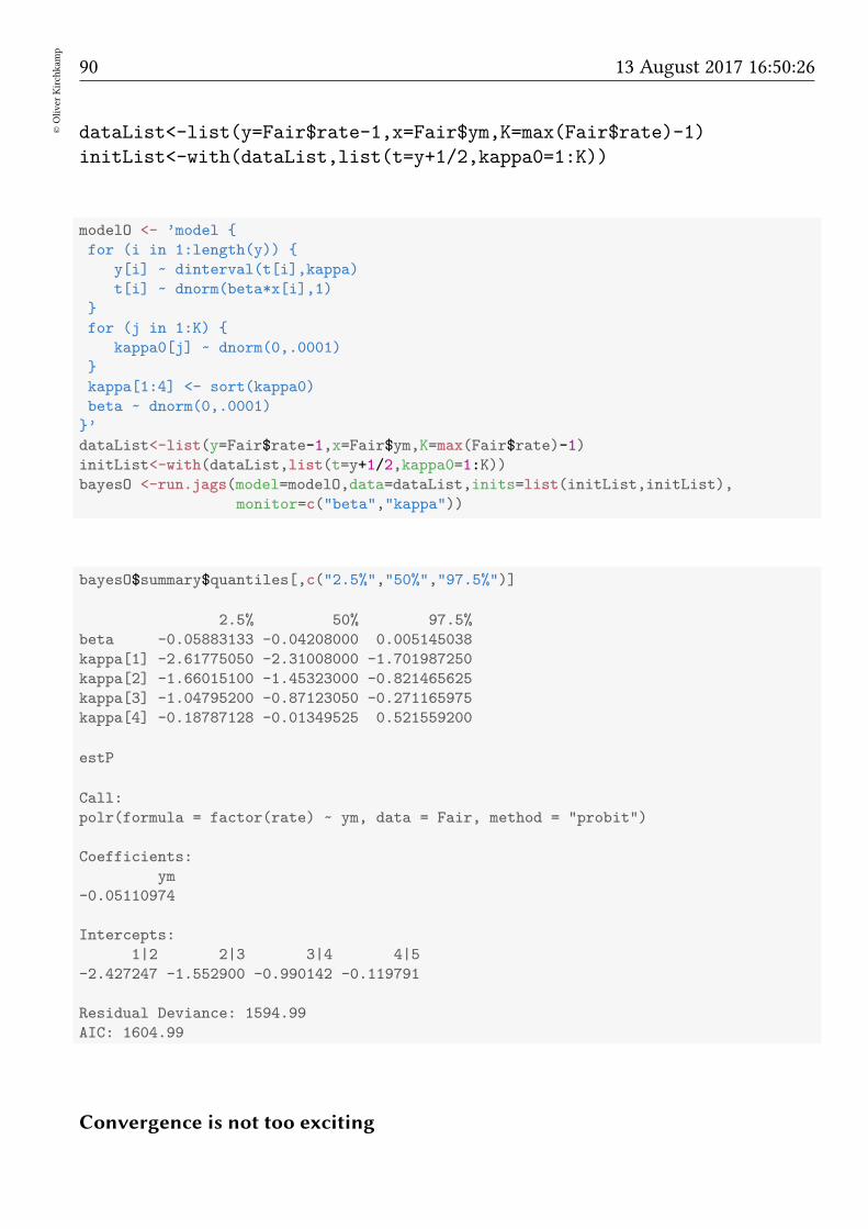
90©Oliver

Kirchkam

p

13 August 2017 16:50:26

dataList<-list(y=Fair$rate-1,x=Fair$ym,K=max(Fair$rate)-1)

initList<-with(dataList,list(t=y+1/2,kappa0=1:K))

modelO <- ’model


y[i] ~ dinterval(t[i],kappa)

t[i] ~ dnorm(beta*x[i],1)

for (j in 1:K)

kappa0[j] ~ dnorm(0,.0001)

kappa[1:4] <- sort(kappa0)

beta ~ dnorm(0,.0001)

’

dataList<-list(y=Fair$rate-1,x=Fair$ym,K=max(Fair$rate)-1)

initList<-with(dataList,list(t=y+1/2,kappa0=1:K))

bayesO <-run.jags(model=modelO,data=dataList,inits=list(initList,initList),

monitor=c("beta","kappa"))

bayesO$summary$quantiles[,c("2.5%","50%","97.5%")]

2.5% 50% 97.5%

beta -0.05883133 -0.04208000 0.005145038

kappa[1] -2.61775050 -2.31008000 -1.701987250

kappa[2] -1.66015100 -1.45323000 -0.821465625

kappa[3] -1.04795200 -0.87123050 -0.271165975

kappa[4] -0.18787128 -0.01349525 0.521559200

estP

Call:

polr(formula = factor(rate) ~ ym, data = Fair, method = "probit")

Coefficients:

ym

-0.05110974

Intercepts:

1|2 2|3 3|4 4|5

-2.427247 -1.552900 -0.990142 -0.119791


AIC: 1604.99

Convergence is not too exciting

Contents 91

©Oliver

Kirchkam

p

bayesO



beta -0.061539 -0.04208 -0.0005693 -0.038078 0.016126 -0.047019 0.0057683

kappa[1] -2.6603 -2.3101 -1.7527 -2.2751 0.2228 -2.3448 0.03129

kappa[2] -1.6862 -1.4532 -0.8756 -1.3938 0.21054 -1.5099 0.066847

kappa[3] -1.0938 -0.87123 -0.38771 -0.82444 0.2017 -0.96236 0.077131

kappa[4] -0.24793 -0.013495 0.40045 0.031712 0.17487 -0.060974 0.069547


beta 35.8 8 0.90535 1.2393

kappa[1] 14 51 0.94751 1.1735

kappa[2] 31.8 10 0.99001 1.2485

kappa[3] 38.2 7 0.99305 1.2836

kappa[4] 39.8 6 0.99375 1.2465


12.3 Exercise

Consider the data set Mathlevel from Ecdat.

• Which variables could explain the attained math level.


13 Instrumental variables

The problem:

Y = Xβ+ ǫ but X 0 ǫ

Solution, use instrument Z ⊢ ǫ

1st stage: X = Zγ+ ν

X = Zγ

2nd stage: Y = Xβ+ ǫ

92©Oliver

Kirchkam

p

13 August 2017 16:50:26

set.seed(123)

N<-100

eps<-rnorm(N)

Z<-rnorm(N)

X<- -eps+Z+.5*rnorm(N)

Y<-X + eps

summary(lm(Y~X))

Call:

lm(formula = Y ~ X)

Residuals:


-1.59416 -0.42295 -0.00768 0.45972 1.88043

Coefficients:


(Intercept) 0.03257 0.06706 0.486 0.628

X 0.58001 0.04503 12.881 <2e-16 ***

---

Signif. codes: 0 ’***’ 0.001 ’**’ 0.01 ’*’ 0.05 ’.’ 0.1 ’ ’ 1



F-statistic: 165.9 on 1 and 98 DF, p-value: < 2.2e-16

Naïve model: ignore that X 0 ǫ

instNaive.model<-’model

for(i in 1:length(y))

y[i]~dnorm(beta[1]+beta[2]*x[i],tau)

beta[1]~dnorm(0,.0001)

beta[2]~dnorm(0,.0001)


’

ini <- genInit(4)

instNaive.jags<-run.jags(model=instNaive.model,data=list(y=Y,x=X,z=Z),

monitor=c("beta","tau"),inits=ini)

summary(instNaive.jags)[,c("Mean","SD","SSeff","psrf")]

Mean SD SSeff psrf

beta[1] 0.03274741 0.06846955 39339 1.0000189

beta[2] 0.57971640 0.04581343 38130 0.9999869

tau 2.20708778 0.30908647 12778 1.0001239

Contents 93

©Oliver

Kirchkam

p

Instrument Z ⊢ ǫ

inst.model<-’model


x[i] ~ dnorm(xHat[i],tau[2]) # 1st stage

xHat[i]<- gamma[1]+gamma[2]*z[i]

y[i] ~ dnorm(beta[1]+beta[2]*xHat[i],tau[1]) # 2nd stage

for(k in 1:2)

beta[k] ~ dnorm(0,.0001)

gamma[k]~ dnorm(0,.0001)

tau[k] ~ dgamma(m[k]^2/d[k]^2,m[k]/d[k]^2); m[k] ~ dexp(1); d[k] ~ dexp(1);

’

inst.jags<-run.jags(model=inst.model,data=list(y=Y,x=X,z=Z),


summary(inst.jags)[,c("Mean","SD","SSeff","psrf")]

Mean SD SSeff psrf

beta[1] 0.08822246 0.1224222 3465 1.001245

beta[2] 0.97934413 0.1204707 3588 1.000527

tau[1] 4.19849540 0.5962644 11327 1.000033

tau[2] 0.85500640 0.1194926 18651 1.000030

13.1 Example: Demand and Supply

Q

P

D1

D2

D3

S1

S2

S3

Q

P

D1

S1

S2

S3

How can we estimate the slope of D, if D and S are moving simultaneously?

94©Oliver

Kirchkam

p

13 August 2017 16:50:26

The Demand for Cigarees

The dataset

• state: Factor indicating state.

• year: Factor indicating year.

• cpi: Consumer price index.

• population: State population.

• packs: Number of packs per capita.

• income: State personal income (total, nominal).

• tax: Average state, federal and average local excise taxes for fiscal year.

• price: Average price during fiscal year, including sales tax.

• taxs: Average excise taxes for fiscal year, including sales tax.

library(AER)

data("CigarettesSW", package = "AER")

head(CigarettesSW)

state year cpi population packs income tax price taxs

1 AL 1985 1.076 3973000 116.4863 46014968 32.5 102.18167 33.34834

2 AR 1985 1.076 2327000 128.5346 26210736 37.0 101.47500 37.00000

3 AZ 1985 1.076 3184000 104.5226 43956936 31.0 108.57875 36.17042

4 CA 1985 1.076 26444000 100.3630 447102816 26.0 107.83734 32.10400

5 CO 1985 1.076 3209000 112.9635 49466672 31.0 94.26666 31.00000

6 CT 1985 1.076 3201000 109.2784 60063368 42.0 128.02499 51.48333

We have to construct some variables:Clean the data:

Cig <- within(subset(CigarettesSW,year=="1995"),

rprice <- price/cpi

rincome <- income/population/cpi

tdiff <- (taxs - tax)/cpi

rtax <- tax/cpi

)

log(packs) = Y

log(rprice) = X

tdiff = Z

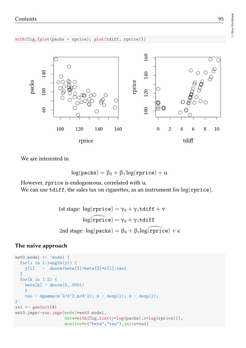
Contents 95

©Oliver

Kirchkam

p

with(Cig,plot(packs ~ rprice); plot(tdiff, rprice))

100 120 140 160

60100

140

rprice

packs

0 2 4 6 8 10

100

120

140

160

tdiffrprice

We are interested in

log(packs) = β0 + β1 log(rprice) + u

However, rprice is endogeneous, correlated with u.We can use tdiff, the sales tax on cigarettes, as an instrument for log(rprice).

1st stage: log(rprice) = γ0 + γ1tdiff + ν

log(rprice) = γ0 + γ1tdiff

2nd stage: log(packs) = β0 + β1log(rprice) + ǫ

The naïve approach

est0.model <- ’model


y[i] ~ dnorm(beta[1]+beta[2]*x[i],tau)

for(k in 1:2)



’

ini <- genInit(4)

est0.jags<-run.jags(model=est0.model,

data=with(Cig,list(y=log(packs),x=log(rprice))),


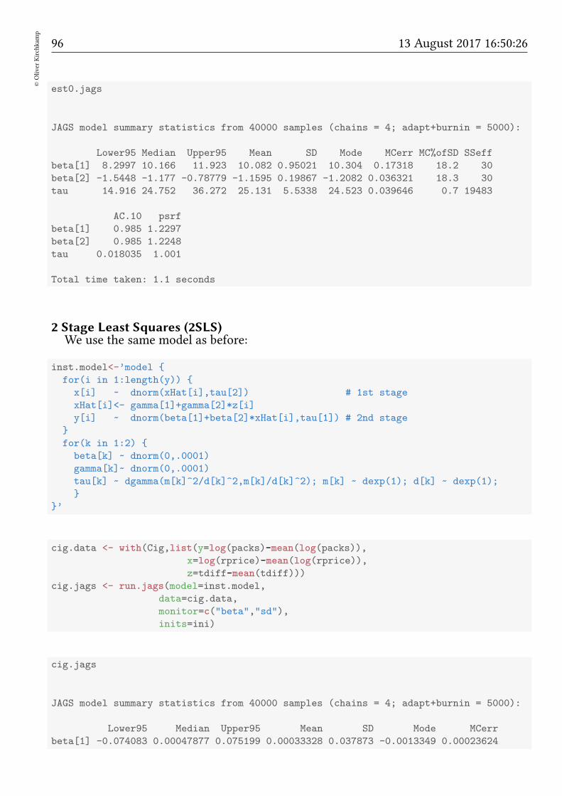
96©Oliver

Kirchkam

p

13 August 2017 16:50:26

est0.jags



beta[1] 8.2997 10.166 11.923 10.082 0.95021 10.304 0.17318 18.2 30

beta[2] -1.5448 -1.177 -0.78779 -1.1595 0.19867 -1.2082 0.036321 18.3 30

tau 14.916 24.752 36.272 25.131 5.5338 24.523 0.039646 0.7 19483

AC.10 psrf

beta[1] 0.985 1.2297

beta[2] 0.985 1.2248

tau 0.018035 1.001


2 Stage Least Squares (2SLS)We use the same model as before:

inst.model<-’model





for(k in 1:2)




’

cig.data <- with(Cig,list(y=log(packs)-mean(log(packs)),

x=log(rprice)-mean(log(rprice)),

z=tdiff-mean(tdiff)))

cig.jags <- run.jags(model=inst.model,

data=cig.data,

monitor=c("beta","sd"),

inits=ini)

cig.jags



beta[1] -0.074083 0.00047877 0.075199 0.00033328 0.037873 -0.0013349 0.00023624

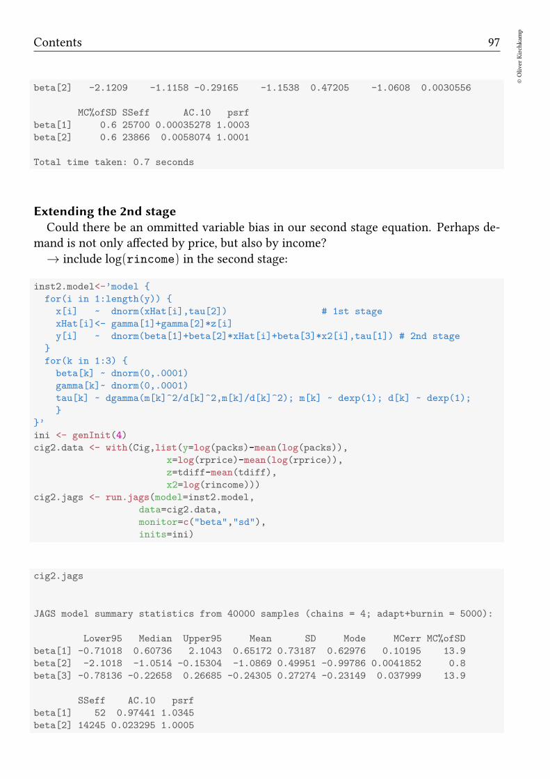
Contents 97

©Oliver

Kirchkam

p

beta[2] -2.1209 -1.1158 -0.29165 -1.1538 0.47205 -1.0608 0.0030556


beta[1] 0.6 25700 0.00035278 1.0003

beta[2] 0.6 23866 0.0058074 1.0001


Extending the 2nd stage

Could there be an ommitted variable bias in our second stage equation. Perhaps de-mand is not only affected by price, but also by income?

→ include log(rincome) in the second stage:

inst2.model<-’model




y[i] ~ dnorm(beta[1]+beta[2]*xHat[i]+beta[3]*x2[i],tau[1]) # 2nd stage

for(k in 1:3)




’

ini <- genInit(4)

cig2.data <- with(Cig,list(y=log(packs)-mean(log(packs)),

x=log(rprice)-mean(log(rprice)),

z=tdiff-mean(tdiff),

x2=log(rincome)))

cig2.jags <- run.jags(model=inst2.model,

data=cig2.data,

monitor=c("beta","sd"),

inits=ini)

cig2.jags



beta[1] -0.71018 0.60736 2.1043 0.65172 0.73187 0.62976 0.10195 13.9

beta[2] -2.1018 -1.0514 -0.15304 -1.0869 0.49951 -0.99786 0.0041852 0.8

beta[3] -0.78136 -0.22658 0.26685 -0.24305 0.27274 -0.23149 0.037999 13.9

SSeff AC.10 psrf

beta[1] 52 0.97441 1.0345

beta[2] 14245 0.023295 1.0005

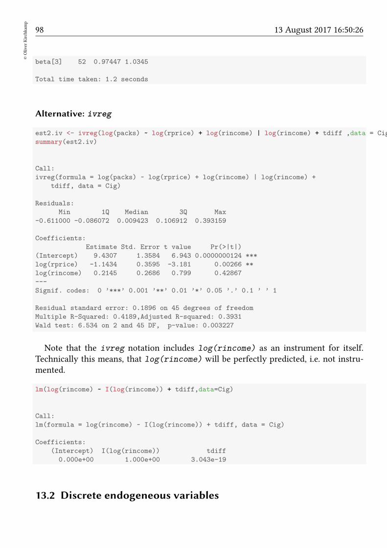
98©Oliver

Kirchkam

p

13 August 2017 16:50:26

beta[3] 52 0.97447 1.0345


Alternative: ivreg

est2.iv <- ivreg(log(packs) ~ log(rprice) + log(rincome) | log(rincome) + tdiff ,data = Cig)

summary(est2.iv)

Call:

ivreg(formula = log(packs) ~ log(rprice) + log(rincome) | log(rincome) +

tdiff, data = Cig)

Residuals:


-0.611000 -0.086072 0.009423 0.106912 0.393159

Coefficients:


(Intercept) 9.4307 1.3584 6.943 0.0000000124 ***

log(rprice) -1.1434 0.3595 -3.181 0.00266 **

log(rincome) 0.2145 0.2686 0.799 0.42867

---

Signif. codes: 0 ’***’ 0.001 ’**’ 0.01 ’*’ 0.05 ’.’ 0.1 ’ ’ 1


Multiple R-Squared: 0.4189,Adjusted R-squared: 0.3931

Wald test: 6.534 on 2 and 45 DF, p-value: 0.003227

Note that the ivreg notation includes log(rincome) as an instrument for itself.Technically this means, that log(rincome) will be perfectly predicted, i.e. not instru-mented.

lm(log(rincome) ~ I(log(rincome)) + tdiff,data=Cig)

Call:

lm(formula = log(rincome) ~ I(log(rincome)) + tdiff, data = Cig)

Coefficients:

(Intercept) I(log(rincome)) tdiff

0.000e+00 1.000e+00 3.043e-19

13.2 Discrete endogeneous variables

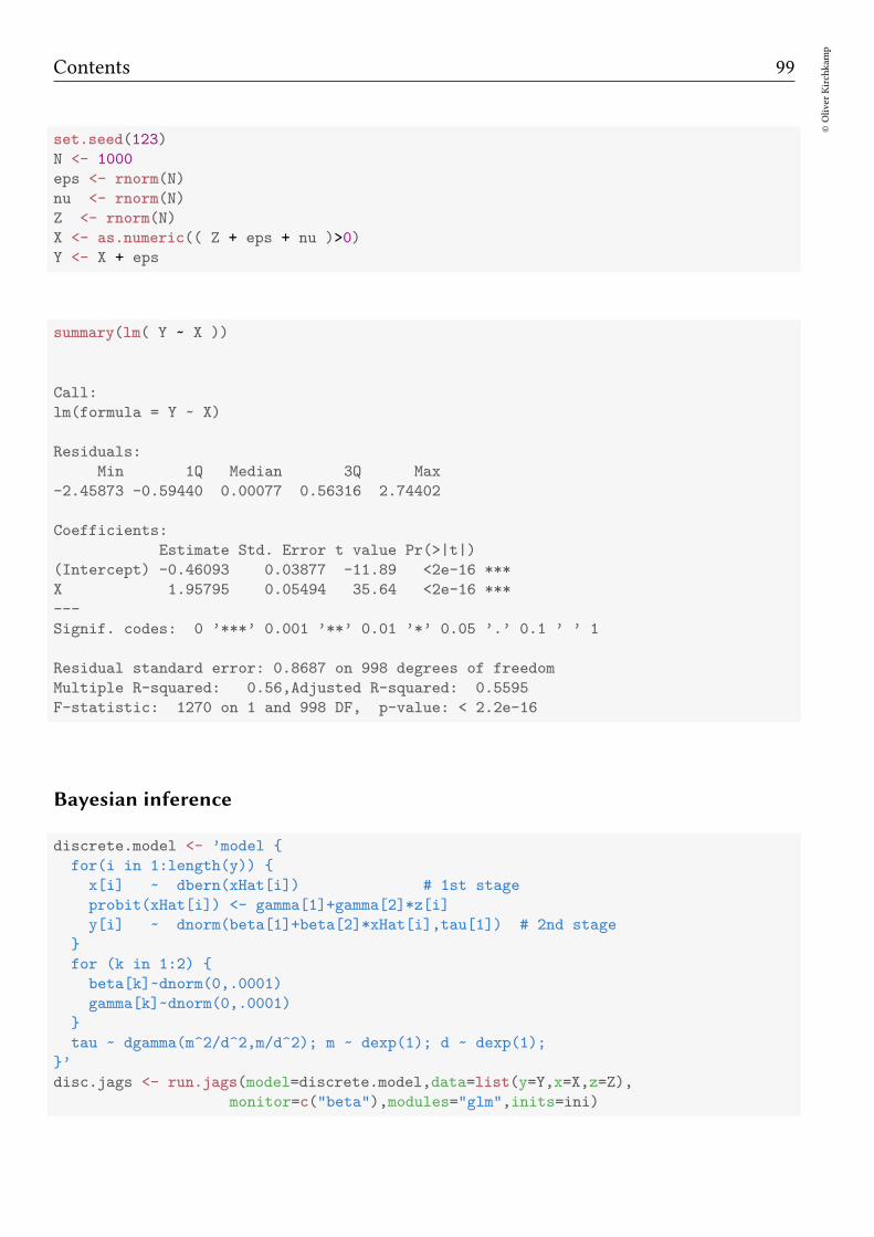
Contents 99

©Oliver

Kirchkam

p

set.seed(123)

N <- 1000

eps <- rnorm(N)

nu <- rnorm(N)

Z <- rnorm(N)

X <- as.numeric(( Z + eps + nu )>0)

Y <- X + eps

summary(lm( Y ~ X ))

Call:

lm(formula = Y ~ X)

Residuals:


-2.45873 -0.59440 0.00077 0.56316 2.74402

Coefficients:


(Intercept) -0.46093 0.03877 -11.89 <2e-16 ***

X 1.95795 0.05494 35.64 <2e-16 ***

---

Signif. codes: 0 ’***’ 0.001 ’**’ 0.01 ’*’ 0.05 ’.’ 0.1 ’ ’ 1



F-statistic: 1270 on 1 and 998 DF, p-value: < 2.2e-16

Bayesian inference

discrete.model <- ’model


x[i] ~ dbern(xHat[i]) # 1st stage

probit(xHat[i]) <- gamma[1]+gamma[2]*z[i]


for (k in 1:2)

beta[k]~dnorm(0,.0001)

gamma[k]~dnorm(0,.0001)


’

disc.jags <- run.jags(model=discrete.model,data=list(y=Y,x=X,z=Z),

monitor=c("beta"),modules="glm",inits=ini)

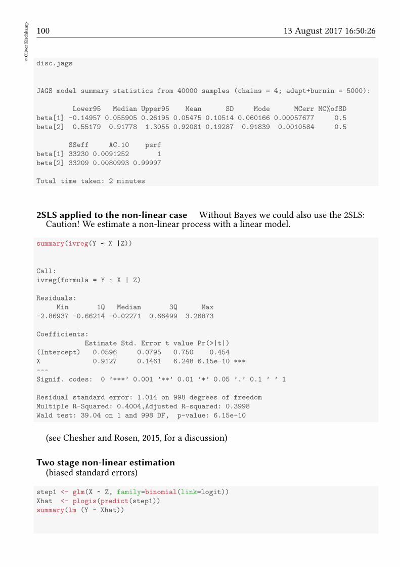
100©Oliver

Kirchkam

p

13 August 2017 16:50:26

disc.jags



beta[1] -0.14957 0.055905 0.26195 0.05475 0.10514 0.060166 0.00057677 0.5

beta[2] 0.55179 0.91778 1.3055 0.92081 0.19287 0.91839 0.0010584 0.5

SSeff AC.10 psrf

beta[1] 33230 0.0091252 1

beta[2] 33209 0.0080993 0.99997

Total time taken: 2 minutes

2SLS applied to the non-linear case Without Bayes we could also use the 2SLS:Caution! We estimate a non-linear process with a linear model.

summary(ivreg(Y ~ X |Z))

Call:

ivreg(formula = Y ~ X | Z)

Residuals:


-2.86937 -0.66214 -0.02271 0.66499 3.26873

Coefficients:


(Intercept) 0.0596 0.0795 0.750 0.454

X 0.9127 0.1461 6.248 6.15e-10 ***

---

Signif. codes: 0 ’***’ 0.001 ’**’ 0.01 ’*’ 0.05 ’.’ 0.1 ’ ’ 1


Multiple R-Squared: 0.4004,Adjusted R-squared: 0.3998

Wald test: 39.04 on 1 and 998 DF, p-value: 6.15e-10

(see Chesher and Rosen, 2015, for a discussion)

Two stage non-linear estimation(biased standard errors)

step1 <- glm(X ~ Z, family=binomial(link=logit))

Xhat <- plogis(predict(step1))

summary(lm (Y ~ Xhat))

Contents 101

©Oliver

Kirchkam

p

Call:

lm(formula = Y ~ Xhat)

Residuals:


-3.3240 -0.9231 -0.0019 0.9277 3.7916

Coefficients:


(Intercept) 0.05804 0.10057 0.577 0.564

Xhat 0.91584 0.18448 4.964 0.00000081 ***

---

Signif. codes: 0 ’***’ 0.001 ’**’ 0.01 ’*’ 0.05 ’.’ 0.1 ’ ’ 1




13.3 Exercises

Consider the data set RetSchool from Ecdat. You want to study the impact of educationon wage.

1. Why could education be endogeneous and why could this be problem?

2. Which variables could be used as instruments?

3. Compare a model with and without instruments.

14 Measurement errors

14.1 Single measures, known error

In OLS we assume that Y is measured only with precision τ, however, X is infinitelyprecise:

Y ∼ N(β0 + β1X, τY)

Assume that X ∼ N(ξ, τη)

We are interested in

Y ∼ N(β0 + β1ξ, τY)

Pretending that X is an infinitely precise measure for ξ leads to a biased estimate ofβ1.

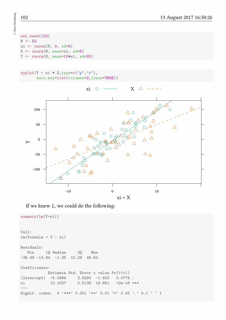
102©Oliver

Kirchkam

p

13 August 2017 16:50:26

set.seed(123)

N <- 50

xi <- rnorm(N, 0, sd=6)

X <- rnorm(N, mean=xi, sd=5)

Y <- rnorm(N, mean=10*xi, sd=20)

xyplot(Y ~ xi + X,type=c("p","r"),

auto.key=list(columns=2,lines=TRUE))

xi + X

Y

-100

-50

0

50

100

-10 0 10

xi X

If we knew ξ, we could do the following:

summary(lm(Y~xi))

Call:

lm(formula = Y ~ xi)

Residuals:


-36.48 -13.64 -1.35 10.29 46.62

Coefficients:


(Intercept) -5.0994 2.8280 -1.803 0.0776 .

xi 10.1037 0.5139 19.661 <2e-16 ***

---

Signif. codes: 0 ’***’ 0.001 ’**’ 0.01 ’*’ 0.05 ’.’ 0.1 ’ ’ 1

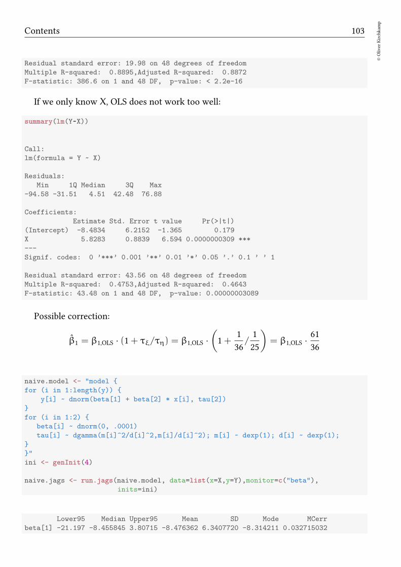
Contents 103

©Oliver

Kirchkam

p



F-statistic: 386.6 on 1 and 48 DF, p-value: < 2.2e-16

If we only know X, OLS does not work too well:

summary(lm(Y~X))

Call:

lm(formula = Y ~ X)

Residuals:


-94.58 -31.51 4.51 42.48 76.88

Coefficients:


(Intercept) -8.4834 6.2152 -1.365 0.179

X 5.8283 0.8839 6.594 0.0000000309 ***

---

Signif. codes: 0 ’***’ 0.001 ’**’ 0.01 ’*’ 0.05 ’.’ 0.1 ’ ’ 1




Possible correction:

β1 = β1,OLS · (1+ τξ/τη) = β1,OLS ·(

1+1

36/1

25

)

= β1,OLS ·61

36

naive.model <- "model


y[i] ~ dnorm(beta[1] + beta[2] * x[i], tau[2])

for (i in 1:2)

beta[i] ~ dnorm(0, .0001)


"

ini <- genInit(4)

naive.jags <- run.jags(naive.model, data=list(x=X,y=Y),monitor=c("beta"),

inits=ini)


beta[1] -21.197 -8.455845 3.80715 -8.476362 6.3407720 -8.314211 0.032715032

104©Oliver

Kirchkam

p

13 August 2017 16:50:26

beta[2] 4.060 5.828210 7.59205 5.832346 0.8989696 5.825623 0.004552546


beta[1] 0.5 37566 0.007309543 1.000062

beta[2] 0.5 38993 -0.005758597 1.000010

The following models allows to specify the measurement error as tau[1]

measure.model <- "model


xi[i] ~ dnorm(0, tau[3])

x[i] ~ dnorm(xi[i], tau[1])

y[i] ~ dnorm(beta[1] + beta[2] * xi[i], tau[2])

for (i in 1:2)



"

We replicate the “naïve” model by setting tau[1]=100.

naive2.jags<-run.jags(measure.model,

data=list(x = X, y = Y, tau=c(100,NA,1/36)),

monitor=c("beta"),inits=ini)

Pretending (as in naive2.jags) that there is no measurement error (tau[1]=100)does not help.


beta[1] -21.18160 -8.48736 3.82251 -8.463209 6.345481 -8.455162 0.032222314

beta[2] 4.09644 5.83252 7.65871 5.829194 0.905098 5.806014 0.004669013


beta[1] 0.5 38781 0.0004631007 1.0000624

beta[2] 0.5 37579 -0.0005470156 0.9999804

Here we set the measurement error to the correct value: tau[1]=1/25.

run.jags(measure.model,data=list(x = X, y = Y, tau=c(1/25,NA,1/36)),




beta[1] -22.867 -8.2852 1.8318 -9.2168 6.4911 -6.9215 0.82292 12.7 62

beta[2] 8.8216 10.764 12.9 10.899 1.0461 10.531 0.12198 11.7 74

AC.10 psrf

beta[1] 0.9225 1.1708

beta[2] 0.92962 1.0342


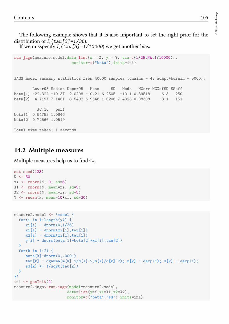
Contents 105

©Oliver

Kirchkam

p

The following example shows that it is also important to set the right prior for thedistribution of ξ (tau[3]=1/36).If we misspecify ξ (tau[3]=1/10000) we get another bias:

run.jags(measure.model,data=list(x = X, y = Y, tau=c(1/25,NA,1/10000)),




beta[1] -22.324 -10.37 2.0408 -10.21 6.2505 -10.1 0.39518 6.3 250

beta[2] 4.7197 7.1481 8.5492 6.9548 1.0206 7.4023 0.08308 8.1 151

AC.10 psrf

beta[1] 0.54753 1.0646

beta[2] 0.72566 1.0519

Total time taken: 1 seconds

14.2 Multiple measures

Multiple measures help us to find τη.

set.seed(123)

N <- 50

xi <- rnorm(N, 0, sd=6)

X1 <- rnorm(N, mean=xi, sd=5)

X2 <- rnorm(N, mean=xi, sd=5)

Y <- rnorm(N, mean=10*xi, sd=20)

measure2.model <- ’model


xi[i] ~ dnorm(0,1/36)

x1[i] ~ dnorm(xi[i],tau[1])

x2[i] ~ dnorm(xi[i],tau[1])

y[i] ~ dnorm(beta[1]+beta[2]*xi[i],tau[2])

for(k in 1:2)

beta[k]~dnorm(0,.0001)


sd[k] <- 1/sqrt(tau[k])

’

ini <- genInit(4)

measure2.jags<-run.jags(model=measure2.model,

data=list(y=Y,x1=X1,x2=X2),

monitor=c("beta","sd"),inits=ini)

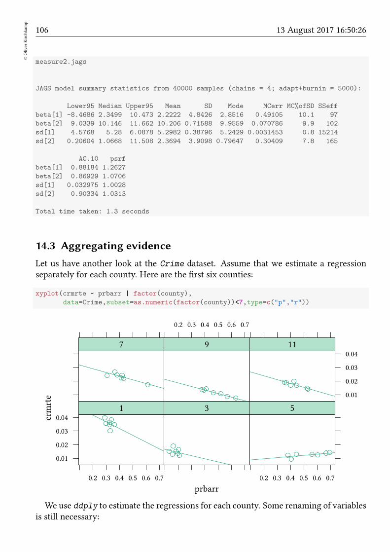
106©Oliver

Kirchkam

p

13 August 2017 16:50:26

measure2.jags



beta[1] -8.4686 2.3499 10.473 2.2222 4.8426 2.8516 0.49105 10.1 97

beta[2] 9.0339 10.146 11.662 10.206 0.71588 9.9559 0.070786 9.9 102

sd[1] 4.5768 5.28 6.0878 5.2982 0.38796 5.2429 0.0031453 0.8 15214

sd[2] 0.20604 1.0668 11.508 2.3694 3.9098 0.79647 0.30409 7.8 165

AC.10 psrf

beta[1] 0.88184 1.2627

beta[2] 0.86929 1.0706

sd[1] 0.032975 1.0028

sd[2] 0.90334 1.0313


14.3 Aggregating evidence

Let us have another look at the Crime dataset. Assume that we estimate a regressionseparately for each county. Here are the first six counties:

xyplot(crmrte ~ prbarr | factor(county),

data=Crime,subset=as.numeric(factor(county))<7,type=c("p","r"))

prbarr

crmrte

0.01

0.02

0.03

0.04

0.2 0.3 0.4 0.5 0.6 0.7

1 3

0.2 0.3 0.4 0.5 0.6 0.7

5

7

0.2 0.3 0.4 0.5 0.6 0.7

9

0.01

0.02

0.03

0.0411

We use ddply to estimate the regressions for each county. Some renaming of variablesis still necessary:

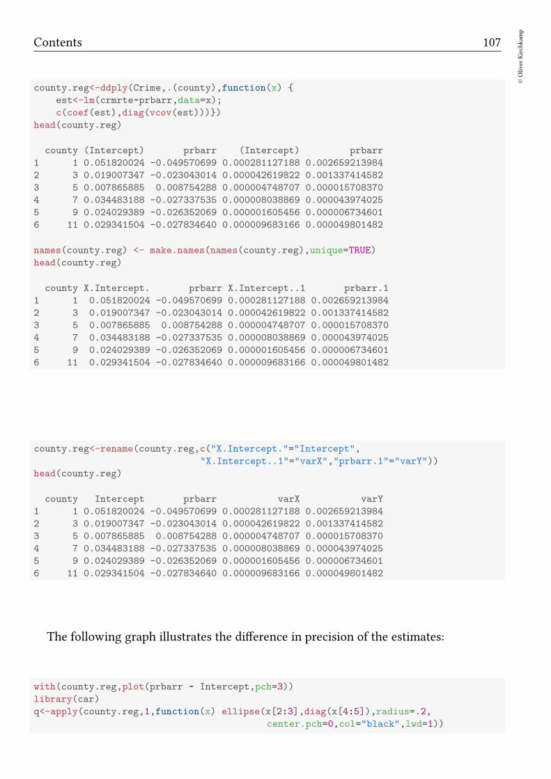
Contents 107

©Oliver

Kirchkam

p

county.reg<-ddply(Crime,.(county),function(x)

est<-lm(crmrte~prbarr,data=x);

c(coef(est),diag(vcov(est))))

head(county.reg)

county (Intercept) prbarr (Intercept) prbarr

1 1 0.051820024 -0.049570699 0.000281127188 0.002659213984

2 3 0.019007347 -0.023043014 0.000042619822 0.001337414582

3 5 0.007865885 0.008754288 0.000004748707 0.000015708370

4 7 0.034483188 -0.027337535 0.000008038869 0.000043974025

5 9 0.024029389 -0.026352069 0.000001605456 0.000006734601

6 11 0.029341504 -0.027834640 0.000009683166 0.000049801482

names(county.reg) <- make.names(names(county.reg),unique=TRUE)

head(county.reg)

county X.Intercept. prbarr X.Intercept..1 prbarr.1

1 1 0.051820024 -0.049570699 0.000281127188 0.002659213984

2 3 0.019007347 -0.023043014 0.000042619822 0.001337414582

3 5 0.007865885 0.008754288 0.000004748707 0.000015708370

4 7 0.034483188 -0.027337535 0.000008038869 0.000043974025

5 9 0.024029389 -0.026352069 0.000001605456 0.000006734601

6 11 0.029341504 -0.027834640 0.000009683166 0.000049801482

county.reg<-rename(county.reg,c("X.Intercept."="Intercept",

"X.Intercept..1"="varX","prbarr.1"="varY"))

head(county.reg)

county Intercept prbarr varX varY

1 1 0.051820024 -0.049570699 0.000281127188 0.002659213984

2 3 0.019007347 -0.023043014 0.000042619822 0.001337414582

3 5 0.007865885 0.008754288 0.000004748707 0.000015708370

4 7 0.034483188 -0.027337535 0.000008038869 0.000043974025

5 9 0.024029389 -0.026352069 0.000001605456 0.000006734601

6 11 0.029341504 -0.027834640 0.000009683166 0.000049801482

The following graph illustrates the difference in precision of the estimates:

with(county.reg,plot(prbarr ~ Intercept,pch=3))

library(car)

q<-apply(county.reg,1,function(x) ellipse(x[2:3],diag(x[4:5]),radius=.2,

center.pch=0,col="black",lwd=1))

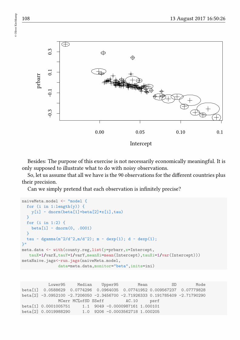
108©Oliver

Kirchkam

p

13 August 2017 16:50:26

0.00 0.05 0.10 0.15

-0.3

-0.1

0.1

0.3

Intercept

prbarr

Besides: The purpose of this exercise is not necessarily economically meaningful. It isonly supposed to illustrate what to do with noisy observations.

So, let us assume that all we have is the 90 observations for the different countries plustheir precision.

Can we simply pretend that each observation is infinitely precise?

naiveMeta.model <- "model


y[i] ~ dnorm(beta[1]+beta[2]*x[i],tau)

for (i in 1:2)



"

meta.data <- with(county.reg,list(y=prbarr,x=Intercept,

tauX=1/varX,tauY=1/varY,meanXi=mean(Intercept),tauXi=1/var(Intercept)))

metaNaive.jags<-run.jags(naiveMeta.model,

data=meta.data,monitor="beta",inits=ini)


beta[1] 0.0588629 0.0774296 0.0964035 0.07741952 0.009567237 0.07779828

beta[2] -3.0952100 -2.7206050 -2.3456700 -2.71926333 0.191785409 -2.71790290


beta[1] 0.0001005751 1.1 9049 -0.0000987161 1.000101

beta[2] 0.0019988290 1.0 9206 -0.0003562718 1.000205

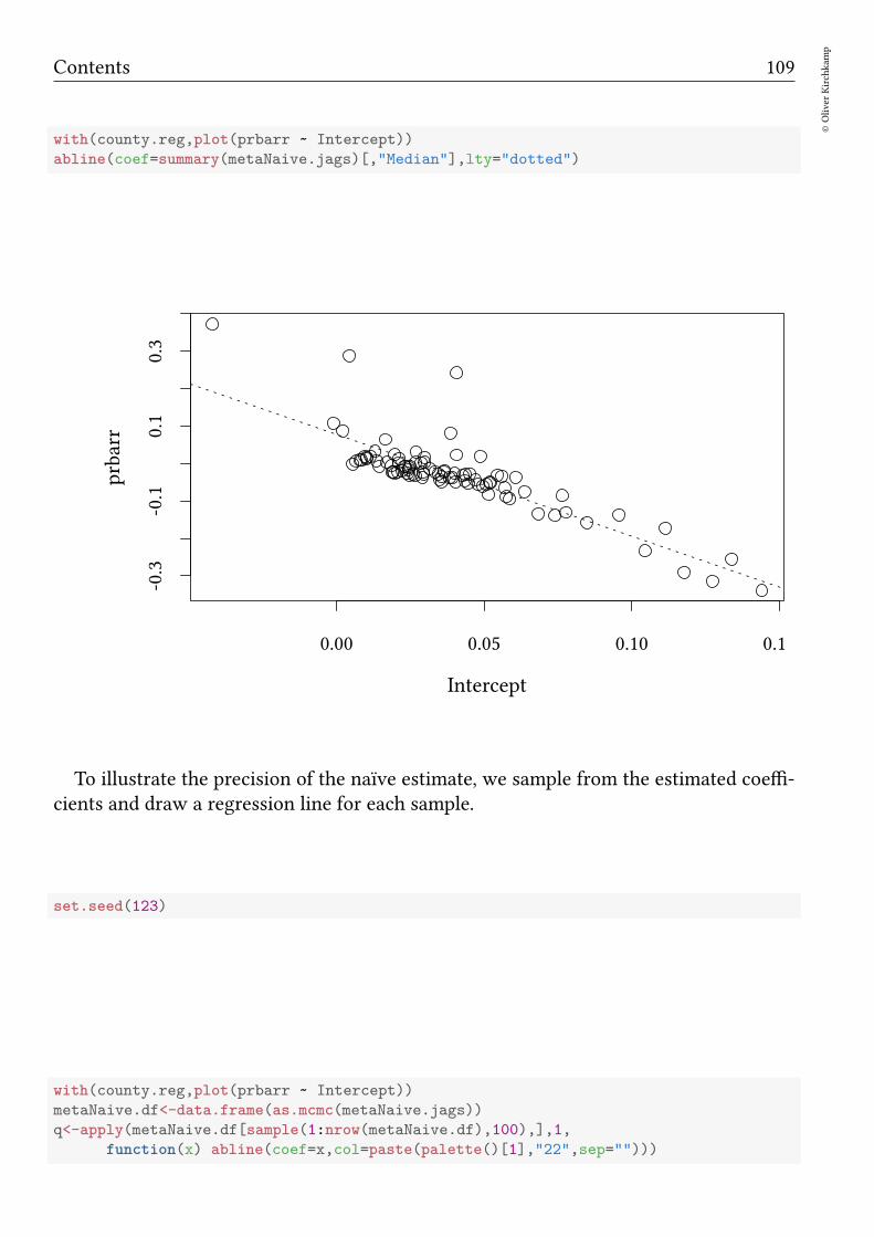
Contents 109

©Oliver

Kirchkam

p

with(county.reg,plot(prbarr ~ Intercept))

abline(coef=summary(metaNaive.jags)[,"Median"],lty="dotted")

0.00 0.05 0.10 0.15

-0.3

-0.1

0.1

0.3

Intercept

prbarr

To illustrate the precision of the naïve estimate, we sample from the estimated coeffi-cients and draw a regression line for each sample.

set.seed(123)


metaNaive.df<-data.frame(as.mcmc(metaNaive.jags))

q<-apply(metaNaive.df[sample(1:nrow(metaNaive.df),100),],1,

function(x) abline(coef=x,col=paste(palette()[1],"22",sep="")))

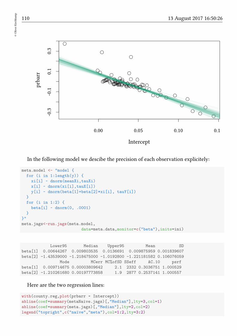
110©Oliver

Kirchkam

p

13 August 2017 16:50:26

0.00 0.05 0.10 0.15

-0.3

-0.1

0.1

0.3

Intercept

prbarr

In the following model we descibe the precision of each observation explicitely:

meta.model <- "model


xi[i] ~ dnorm(meanXi,tauXi)

x[i] ~ dnorm(xi[i],tauX[i])

y[i] ~ dnorm(beta[1]+beta[2]*xi[i], tauY[i])

for (i in 1:2)


"

meta.jags<-run.jags(meta.model,

data=meta.data,monitor=c("beta"),inits=ini)

Lower95 Median Upper95 Mean SD

beta[1] 0.00644267 0.009803535 0.0136691 0.009875959 0.001839607

beta[2] -1.43539000 -1.218475000 -1.0192800 -1.221181582 0.106076059

Mode MCerr MC%ofSD SSeff AC.10 psrf

beta[1] 0.009714675 0.00003809642 2.1 2332 0.3036751 1.000529

beta[2] -1.210261680 0.00197773858 1.9 2877 0.2537141 1.000557

Here are the two regression lines:


abline(coef=summary(metaNaive.jags)[,"Median"],lty=3,col=1)

abline(coef=summary(meta.jags)[,"Median"],lty=2,col=2)

legend("topright",c("naïve","meta"),col=1:2,lty=3:2)

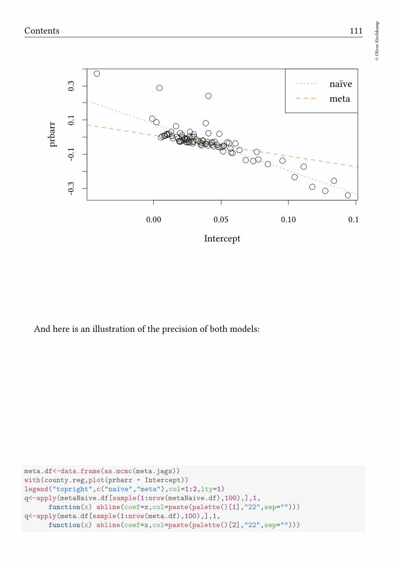
Contents 111

©Oliver

Kirchkam

p

0.00 0.05 0.10 0.15

-0.3

-0.1

0.1

0.3

Intercept

prbarr

naıve

meta

And here is an illustration of the precision of both models:

meta.df<-data.frame(as.mcmc(meta.jags))


legend("topright",c("naïve","meta"),col=1:2,lty=1)

q<-apply(metaNaive.df[sample(1:nrow(metaNaive.df),100),],1,


q<-apply(meta.df[sample(1:nrow(meta.df),100),],1,


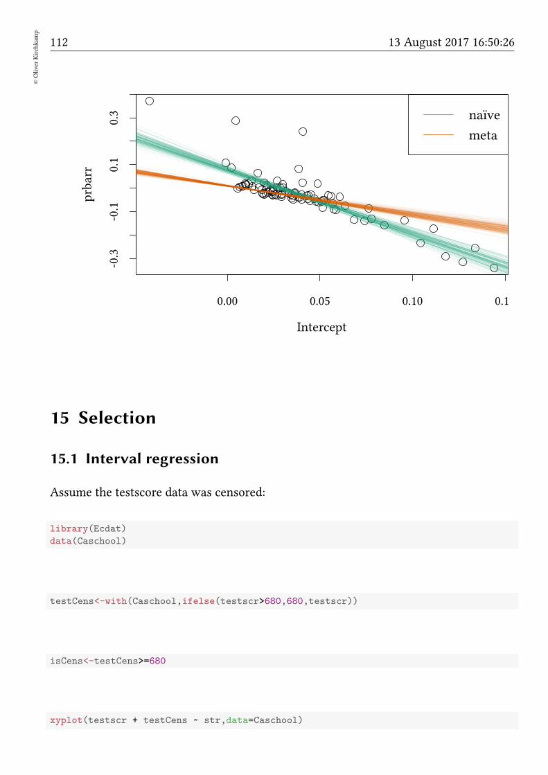
112©Oliver

Kirchkam

p

13 August 2017 16:50:26

0.00 0.05 0.10 0.15

-0.3

-0.1

0.1

0.3

Intercept

prbarr

naıve

meta

15 Selection

15.1 Interval regression

Assume the testscore data was censored:

library(Ecdat)

data(Caschool)

testCens<-with(Caschool,ifelse(testscr>680,680,testscr))

isCens<-testCens>=680

xyplot(testscr + testCens ~ str,data=Caschool)

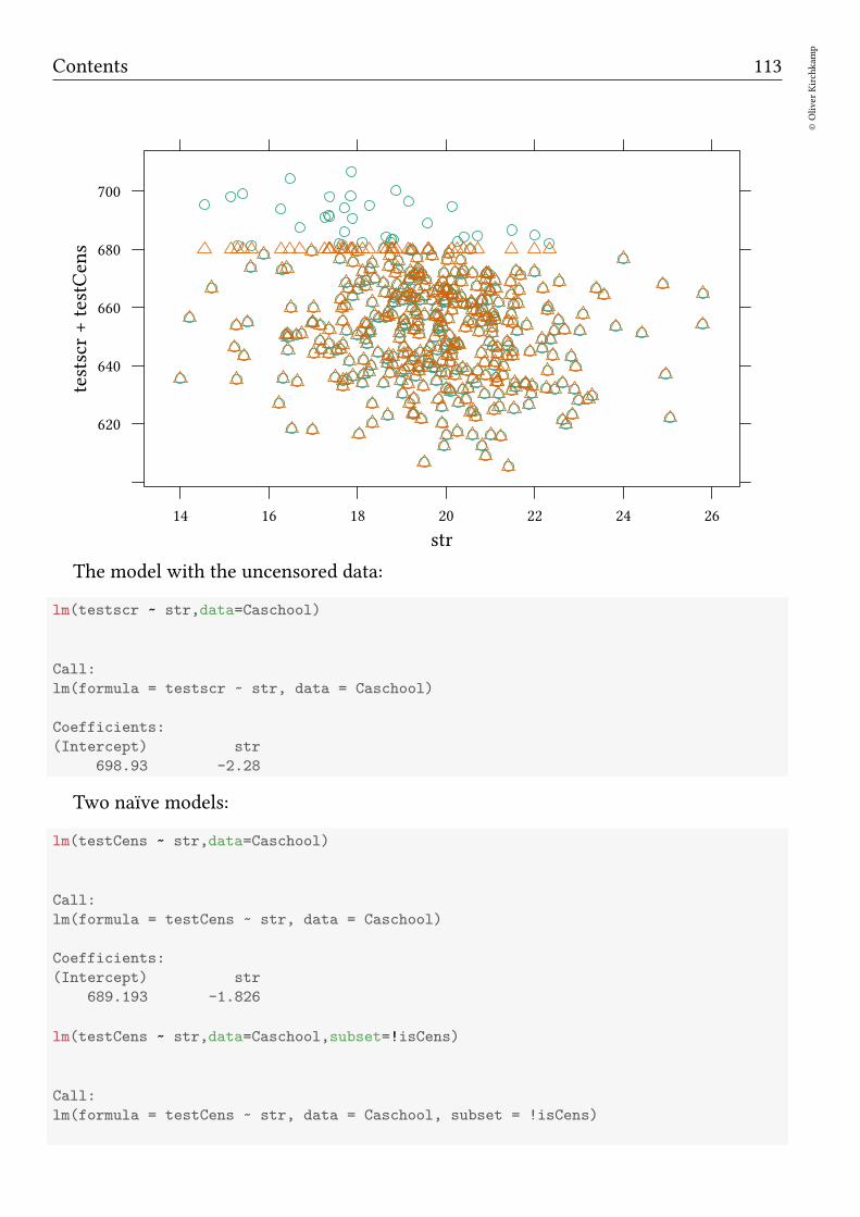
Contents 113

©Oliver

Kirchkam

p

str

testscr+testCens

620

640

660

680

700

14 16 18 20 22 24 26

The model with the uncensored data:

lm(testscr ~ str,data=Caschool)

Call:

lm(formula = testscr ~ str, data = Caschool)

Coefficients:

(Intercept) str

698.93 -2.28

Two naïve models:

lm(testCens ~ str,data=Caschool)

Call:

lm(formula = testCens ~ str, data = Caschool)

Coefficients:

(Intercept) str

689.193 -1.826

lm(testCens ~ str,data=Caschool,subset=!isCens)

Call:

lm(formula = testCens ~ str, data = Caschool, subset = !isCens)

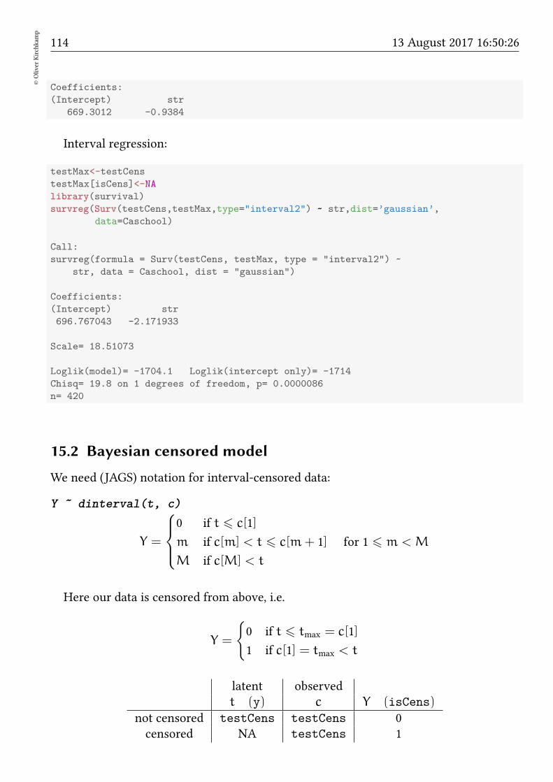
114©Oliver

Kirchkam

p

13 August 2017 16:50:26

Coefficients:

(Intercept) str

669.3012 -0.9384

Interval regression:

testMax<-testCens

testMax[isCens]<-NA

library(survival)

survreg(Surv(testCens,testMax,type="interval2") ~ str,dist=’gaussian’,

data=Caschool)

Call:

survreg(formula = Surv(testCens, testMax, type = "interval2") ~

str, data = Caschool, dist = "gaussian")

Coefficients:

(Intercept) str

696.767043 -2.171933

Scale= 18.51073

Loglik(model)= -1704.1 Loglik(intercept only)= -1714

Chisq= 19.8 on 1 degrees of freedom, p= 0.0000086

n= 420

15.2 Bayesian censored model

We need (JAGS) notation for interval-censored data:

Y ˜ dinterval(t, c)

Y =

0 if t 6 c[1]

m if c[m] < t 6 c[m+ 1] for 1 6 m <M

M if c[M] < t

Here our data is censored from above, i.e.

Y =

0 if t 6 tmax = c[1]

1 if c[1] = tmax < t

latent observedt (y) c Y (isCens)

not censored testCens testCens 0censored NA testCens 1

Contents 115

©Oliver

Kirchkam

p

One complication with the censored model is that the censored observations are un-known, so JAGSwill fit random values. Unless we help JAGS a little, the initial values willbe inconsistent, i.e. JAGS will randomise values for y which are not in the right interval.We must avoid situations like the following:

• y[1]=800, c[1]=600, isCens[1]=0

Problem: according to isCens[1] we have that y[1]<c[1] with certainty.

• y[1]=400, c[1]=600, isCens[1]=1

Problem: according to isCens[1] we have that y[1]>c[1] with certainty.

Otherwise R would throw the following error:

Observed node inconsistent with unobserved parents at initialization.

Try setting appropriate initial values.

Solution: We set the initial y to “safe” values.For the unobserved (censored) nodes, y=testCens+99.For the observed (uncensored) nodes, we can not overwrite the observed nodes. Hence

the init value is y=NA.

y <- ifelse(isCens,NA,testCens)

yInit <- ifelse(isCens,testCens+99,NA) #<- must resolve initial uncertainty about censored y

dataList<-list(y=y,c=testCens,x=Caschool$str,isCens=as.numeric(isCens))

ini <- genInit(4,function(i)

list(beta0=rnorm(1,0,.001),beta1=rnorm(1,0,.001),y=yInit))

initJags<-list()

initJags[[1]]<-list(.RNG.seed=1,.RNG.name="base::Mersenne-Twister")

initJags[[2]]<-list(.RNG.seed=2,.RNG.name="base::Super-Duper")

initJags[[3]]<-list(.RNG.seed=3,.RNG.name="base::Wichmann-Hill")

initJags[[4]]<-list(.RNG.seed=4,.RNG.name="base::Marsaglia-Multicarry")

genInit <- function(nChains,fn=NULL)

x<-list()

for (i in 1:nChains)

x[[i]]<-initJags[[i]]

if(!is.null(fn))

vals<-fn(i)

lapply(1:length(vals),function(j)

x[[i]][[names(vals)[j]]]<<-vals[[j]])

x

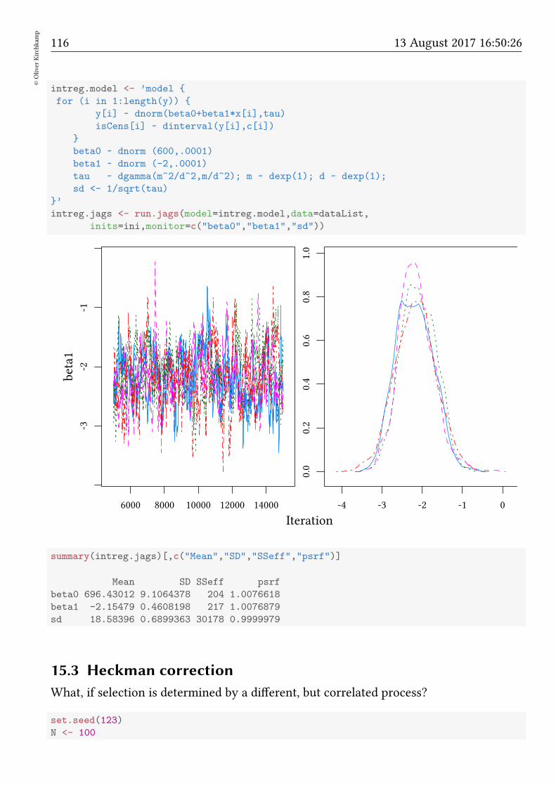
116©Oliver

Kirchkam

p

13 August 2017 16:50:26

intreg.model <- ’model


y[i] ~ dnorm(beta0+beta1*x[i],tau)

isCens[i] ~ dinterval(y[i],c[i])

beta0 ~ dnorm (600,.0001)

beta1 ~ dnorm (-2,.0001)


sd <- 1/sqrt(tau)

’

intreg.jags <- run.jags(model=intreg.model,data=dataList,

inits=ini,monitor=c("beta0","beta1","sd"))

Iteration

beta1

-3-2

-1

6000 8000 10000 12000 14000

0.0

0.2

0.4

0.6

0.8

1.0

-4 -3 -2 -1 0

summary(intreg.jags)[,c("Mean","SD","SSeff","psrf")]

Mean SD SSeff psrf

beta0 696.43012 9.1064378 204 1.0076618

beta1 -2.15479 0.4608198 217 1.0076879

sd 18.58396 0.6899363 30178 0.9999979

15.3 Heckman correction

What, if selection is determined by a different, but correlated process?

set.seed(123)

N <- 100

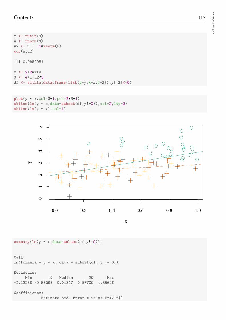
Contents 117

©Oliver

Kirchkam

p

x <- runif(N)

u <- rnorm(N)

u2 <- u + .1*rnorm(N)

cor(u,u2)

[1] 0.9952951

y <- 2+2*x+u

S <- 4*x+u2<3

df <- within(data.frame(list(y=y,x=x,S=S)),y[!S]<-0)

plot(y ~ x,col=S+1,pch=2*S+1)

abline(lm(y ~ x,data=subset(df,y!=0)),col=2,lty=2)

abline(lm(y ~ x),col=1)

0.0 0.2 0.4 0.6 0.8 1.0

01

23

45

6

x

y

summary(lm(y ~ x,data=subset(df,y!=0)))

Call:

lm(formula = y ~ x, data = subset(df, y != 0))

Residuals:


-2.13288 -0.55295 0.01347 0.57709 1.55626

Coefficients:


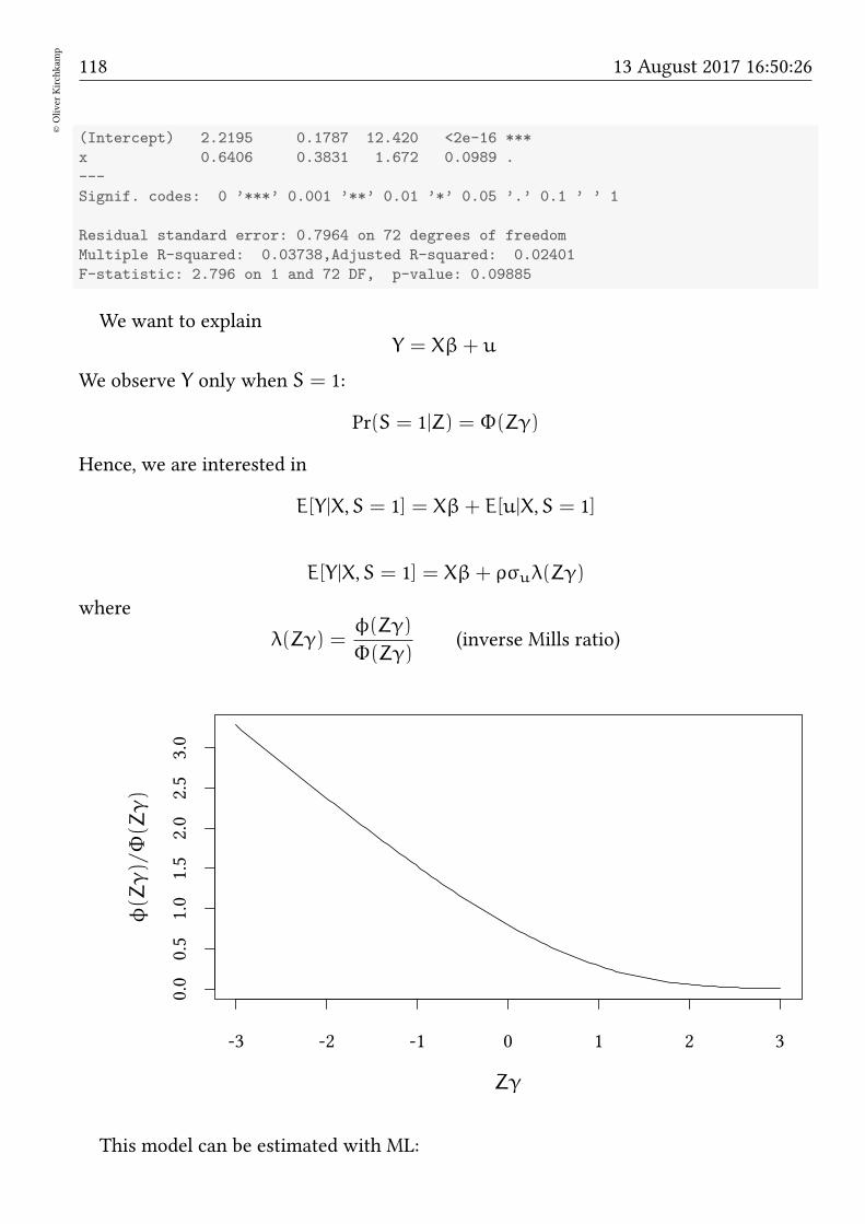
118©Oliver

Kirchkam

p

13 August 2017 16:50:26

(Intercept) 2.2195 0.1787 12.420 <2e-16 ***

x 0.6406 0.3831 1.672 0.0989 .

---

Signif. codes: 0 ’***’ 0.001 ’**’ 0.01 ’*’ 0.05 ’.’ 0.1 ’ ’ 1




We want to explainY = Xβ+ u

We observe Y only when S = 1:

Pr(S = 1|Z) = Φ(Zγ)

Hence, we are interested in

E[Y|X,S = 1] = Xβ+ E[u|X,S = 1]

E[Y|X,S = 1] = Xβ+ ρσuλ(Zγ)

where

λ(Zγ) =φ(Zγ)

Φ(Zγ)(inverse Mills ratio)

-3 -2 -1 0 1 2 3

0.0

0.5

1.0

1.5

2.0

2.5

3.0

Zγ

φ(Zγ)/Φ(Zγ)

This model can be estimated with ML:

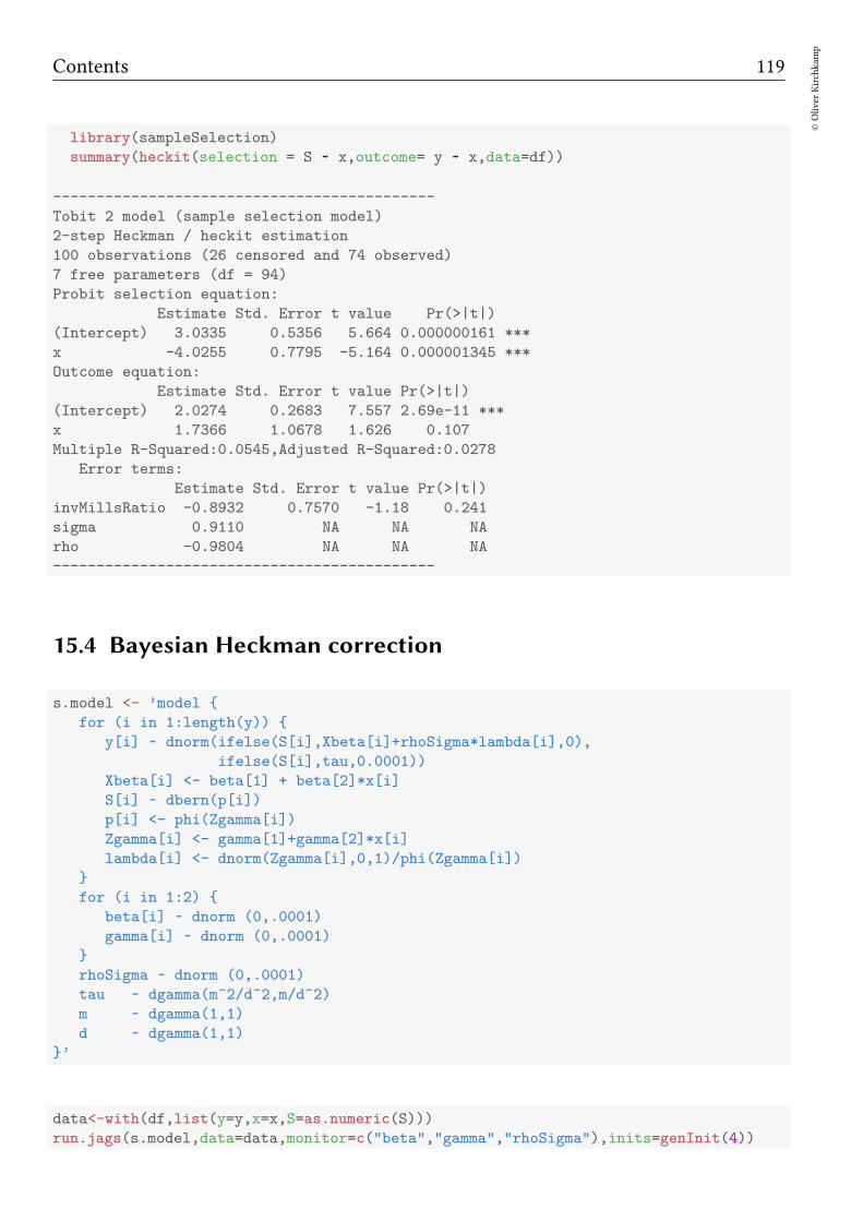
Contents 119

©Oliver

Kirchkam

p

library(sampleSelection)

summary(heckit(selection = S ~ x,outcome= y ~ x,data=df))

--------------------------------------------

Tobit 2 model (sample selection model)

2-step Heckman / heckit estimation

100 observations (26 censored and 74 observed)

7 free parameters (df = 94)

Probit selection equation:


(Intercept) 3.0335 0.5356 5.664 0.000000161 ***

x -4.0255 0.7795 -5.164 0.000001345 ***

Outcome equation:


(Intercept) 2.0274 0.2683 7.557 2.69e-11 ***

x 1.7366 1.0678 1.626 0.107

Multiple R-Squared:0.0545,Adjusted R-Squared:0.0278

Error terms:


invMillsRatio -0.8932 0.7570 -1.18 0.241

sigma 0.9110 NA NA NA

rho -0.9804 NA NA NA

--------------------------------------------

15.4 Bayesian Heckman correction

s.model <- ’model


y[i] ~ dnorm(ifelse(S[i],Xbeta[i]+rhoSigma*lambda[i],0),

ifelse(S[i],tau,0.0001))

Xbeta[i] <- beta[1] + beta[2]*x[i]

S[i] ~ dbern(p[i])

p[i] <- phi(Zgamma[i])

Zgamma[i] <- gamma[1]+gamma[2]*x[i]

lambda[i] <- dnorm(Zgamma[i],0,1)/phi(Zgamma[i])

for (i in 1:2)

beta[i] ~ dnorm (0,.0001)

gamma[i] ~ dnorm (0,.0001)

rhoSigma ~ dnorm (0,.0001)


m ~ dgamma(1,1)

d ~ dgamma(1,1)

’

data<-with(df,list(y=y,x=x,S=as.numeric(S)))

run.jags(s.model,data=data,monitor=c("beta","gamma","rhoSigma"),inits=genInit(4))

120©Oliver

Kirchkam

p

13 August 2017 16:50:26



beta[1] 1.5597 2.0398 2.5262 2.0415 0.24686 2.0216 0.0068395 2.8

beta[2] -0.57032 1.829 4.4669 1.8987 1.2834 1.7863 0.053792 4.2

gamma[1] 1.9511 2.886 3.9597 2.9079 0.52496 2.8471 0.019446 3.7

gamma[2] -5.2501 -3.7935 -2.2889 -3.8196 0.76987 -3.7706 0.028283 3.7

rhoSigma -3.4739 -0.99067 0.99711 -1.1132 1.1601 -0.87304 0.048647 4.2

SSeff AC.10 psrf

beta[1] 1303 0.48573 1.0019

beta[2] 569 0.75123 1.0123

gamma[1] 729 0.68522 1.0032

gamma[2] 741 0.6909 1.0022

rhoSigma 569 0.74052 1.0186


15.5 Exercise

1. Consider the data set Workinghours from Ecdat.

• Which variables could explain the labour supply of the wife?

• In which way could the labour supply be censored?


2. Consider the data set Mroz87 from sampleSelection.

• Explain wage as a function of experience and education.

Assume that selection into the labour force is determinded by age, familyincome and education.

16 More on initialisation

We use different random number generators to make sure that each chain will take adifferent turn.

str(initJags)

List of 4

$ :List of 2

..$ .RNG.seed: num 1

..$ .RNG.name: chr "base::Mersenne-Twister"

$ :List of 2


Contents 121

©Oliver

Kirchkam

p

..$ .RNG.name: chr "base::Super-Duper"

$ :List of 2


..$ .RNG.name: chr "base::Wichmann-Hill"

$ :List of 2


..$ .RNG.name: chr "base::Marsaglia-Multicarry"

The genInit() function helps adding more variables to the init.

genInit <- function(nChains,fn=NULL)

x<-list()

for (i in 1:nChains)

x[[i]]<-initJags[[i]]

if(!is.null(fn))

vals<-fn(i)

lapply(1:length(vals),function(j)

x[[i]][[names(vals)[j]]]<<-vals[[j]])

x

now genInit() can be called like this:

ini <- genInit(4,function(i) list(beta0=rnorm(1,0,0.0001),

beta1=rnorm(1,0,0.0001)))

run.jags(...,inits=ini,...)

17 Hierarchical Models

17.1 Mixed effects

OLS:Yi = Xiβ+ ǫi with ǫ ∼ N(0,σ)

Mixed effects (with groups k):

Yik = Xikβ︸︷︷︸fixed

+ Zikν︸︷︷︸random

+ǫik with ν ∼ N(0,Σ), ǫ ∼ N(0,σ)

17.2 Example: Crime in North Carolina

The dataset Crime contains information about several years. Perhaps the relationshipbetween crmrte and prbarr is not the same in each year?

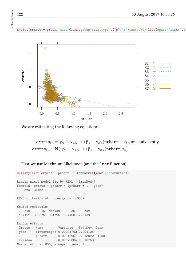
122©Oliver

Kirchkam

p

13 August 2017 16:50:26

xyplot(crmrte ~ prbarr,data=Crime,group=year,type=c("p","r"),auto.key=list(space="right",lines

prbarr

crmrte

0.00

0.05

0.10

0.15

0.0 0.5 1.0 1.5 2.0 2.5

81828384858687

We are estimating the following equation:

crmrteik =(β1 + ν1,k) + (β2 + ν2,k)prbarr + ǫik or, equivalently,

crmrteik ∼ N(

(β1 + ν1,k) + (β2 + ν2,k)prbarr, τ3)

First we use Maximum Likelihood (and the lmer function).

summary(lmer(crmrte ~ prbarr + (prbarr+1|year),data=Crime))

Linear mixed model fit by REML [’lmerMod’]

Formula: crmrte ~ prbarr + (prbarr + 1 | year)

Data: Crime

REML criterion at convergence: -3339

Scaled residuals:


-1.7122 -0.6575 -0.1795 0.4460 7.3139

Random effects:

Groups Name Variance Std.Dev. Corr

year (Intercept) 0.00001702 0.004125

prbarr 0.00016957 0.013022 -1.00

Residual 0.00028084 0.016758

Number of obs: 630, groups: year, 7

Contents 123

©Oliver

Kirchkam

p

Fixed effects:

Estimate Std. Error t value

(Intercept) 0.045302 0.002156 21.012

prbarr -0.044918 0.006579 -6.827

Correlation of Fixed Effects:

(Intr)

prbarr -0.951

17.3 Bayes and mixed effects

Next we specify the mixed model as a JAGS model (since we are mainly interested in themarginal effect, we de-mean crmrte and prbarr).

mer.model <- ’model


y[i] ~ dnorm(mu[i],tau[3])

mu[i]<-beta[1]+nu[1,group[i]]+(beta[2]+nu[2,group[i]])*x[i]

for (k in 1:2)


for (j in 1:max(group))

nu[k,j] ~ dnorm(0,tau[k])

for (k in 1:3)

tau[k] ~ dgamma(.01,.01)

sd[k] <- sqrt(1/tau[k])

’

dataList<-with(Crime,list(y=crmrte-mean(crmrte),x=prbarr-mean(prbarr),

group=as.numeric(year)))

mer.jags<-run.jags(model=mer.model,data=dataList,inits=ini,

monitor=c("beta","sd"))

plot(mer.jags,vars="beta[2]",plot.type=c("trace","density"))

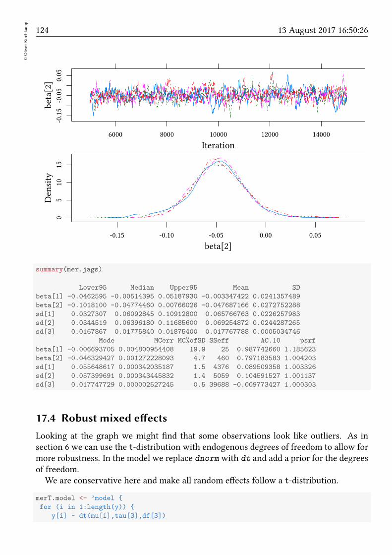
124©Oliver

Kirchkam

p

13 August 2017 16:50:26

Iteration

beta[2]

-0.15

-0.05

0.05

6000 8000 10000 12000 14000

beta[2]

Density

05

1015

-0.15 -0.10 -0.05 0.00 0.05

summary(mer.jags)


beta[1] -0.0462595 -0.00514395 0.05187930 -0.003347422 0.0241357489

beta[2] -0.1018100 -0.04774460 0.00766026 -0.047687166 0.0272752288

sd[1] 0.0327307 0.06092845 0.10912800 0.065766763 0.0226257983

sd[2] 0.0344519 0.06396180 0.11685600 0.069254872 0.0244287265

sd[3] 0.0167867 0.01775840 0.01875400 0.017767788 0.0005034746


beta[1] -0.006693705 0.004800954408 19.9 25 0.987742660 1.185623

beta[2] -0.046329427 0.001272228093 4.7 460 0.797183583 1.004203

sd[1] 0.055648617 0.000342035187 1.5 4376 0.089509358 1.003326

sd[2] 0.057399691 0.000343445832 1.4 5059 0.104591527 1.001137

sd[3] 0.017747729 0.000002527245 0.5 39688 -0.009773427 1.000303

17.4 Robust mixed effects

Looking at the graph we might find that some observations look like outliers. As insection 6 we can use the t-distribution with endogenous degrees of freedom to allow formore robustness. In the model we replace dnorm with dt and add a prior for the degreesof freedom.

We are conservative here and make all random effects follow a t-distribution.

merT.model <- ’model


y[i] ~ dt(mu[i],tau[3],df[3])

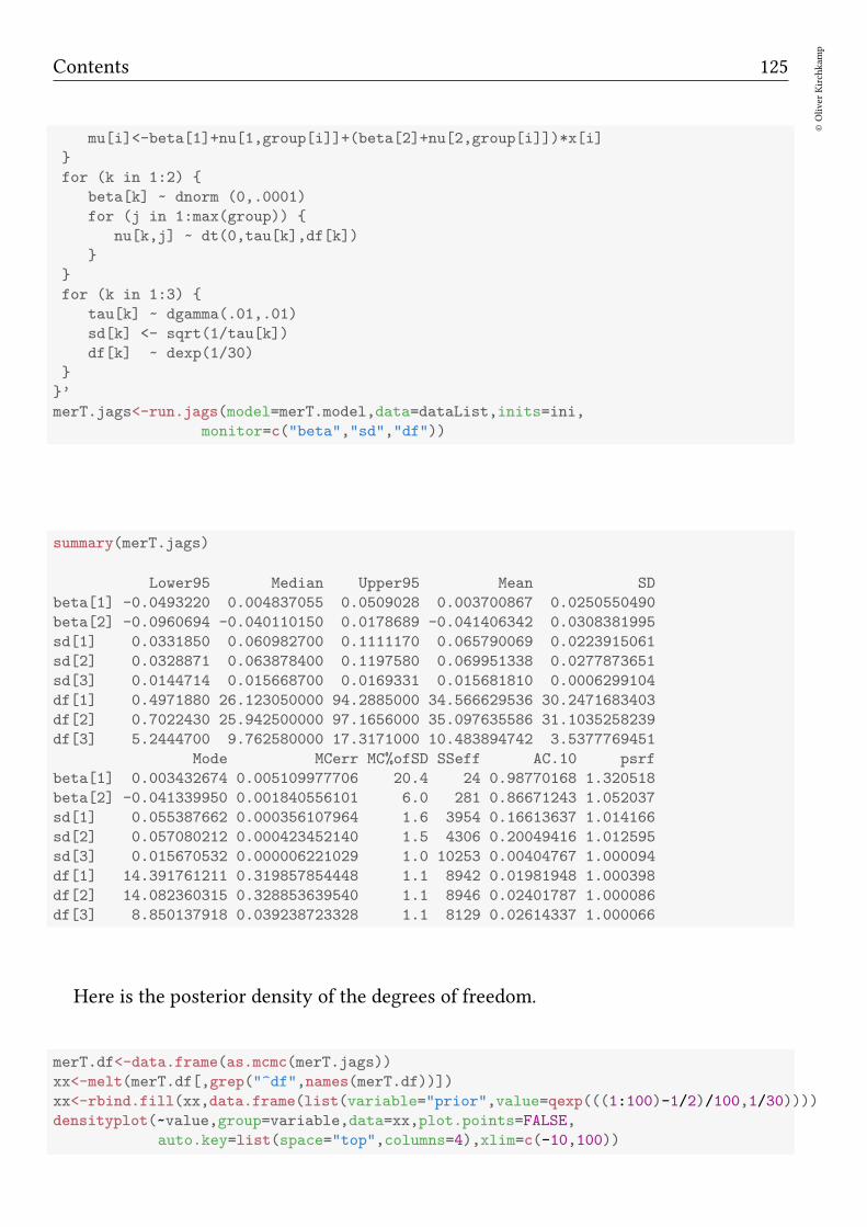
Contents 125

©Oliver

Kirchkam

p

mu[i]<-beta[1]+nu[1,group[i]]+(beta[2]+nu[2,group[i]])*x[i]

for (k in 1:2)


for (j in 1:max(group))

nu[k,j] ~ dt(0,tau[k],df[k])

for (k in 1:3)

tau[k] ~ dgamma(.01,.01)

sd[k] <- sqrt(1/tau[k])

df[k] ~ dexp(1/30)

’

merT.jags<-run.jags(model=merT.model,data=dataList,inits=ini,

monitor=c("beta","sd","df"))

summary(merT.jags)


beta[1] -0.0493220 0.004837055 0.0509028 0.003700867 0.0250550490

beta[2] -0.0960694 -0.040110150 0.0178689 -0.041406342 0.0308381995

sd[1] 0.0331850 0.060982700 0.1111170 0.065790069 0.0223915061

sd[2] 0.0328871 0.063878400 0.1197580 0.069951338 0.0277873651

sd[3] 0.0144714 0.015668700 0.0169331 0.015681810 0.0006299104

df[1] 0.4971880 26.123050000 94.2885000 34.566629536 30.2471683403

df[2] 0.7022430 25.942500000 97.1656000 35.097635586 31.1035258239

df[3] 5.2444700 9.762580000 17.3171000 10.483894742 3.5377769451


beta[1] 0.003432674 0.005109977706 20.4 24 0.98770168 1.320518

beta[2] -0.041339950 0.001840556101 6.0 281 0.86671243 1.052037

sd[1] 0.055387662 0.000356107964 1.6 3954 0.16613637 1.014166

sd[2] 0.057080212 0.000423452140 1.5 4306 0.20049416 1.012595

sd[3] 0.015670532 0.000006221029 1.0 10253 0.00404767 1.000094

df[1] 14.391761211 0.319857854448 1.1 8942 0.01981948 1.000398

df[2] 14.082360315 0.328853639540 1.1 8946 0.02401787 1.000086

df[3] 8.850137918 0.039238723328 1.1 8129 0.02614337 1.000066

Here is the posterior density of the degrees of freedom.

merT.df<-data.frame(as.mcmc(merT.jags))

xx<-melt(merT.df[,grep("^df",names(merT.df))])

xx<-rbind.fill(xx,data.frame(list(variable="prior",value=qexp(((1:100)-1/2)/100,1/30))))

densityplot(~value,group=variable,data=xx,plot.points=FALSE,

auto.key=list(space="top",columns=4),xlim=c(-10,100))

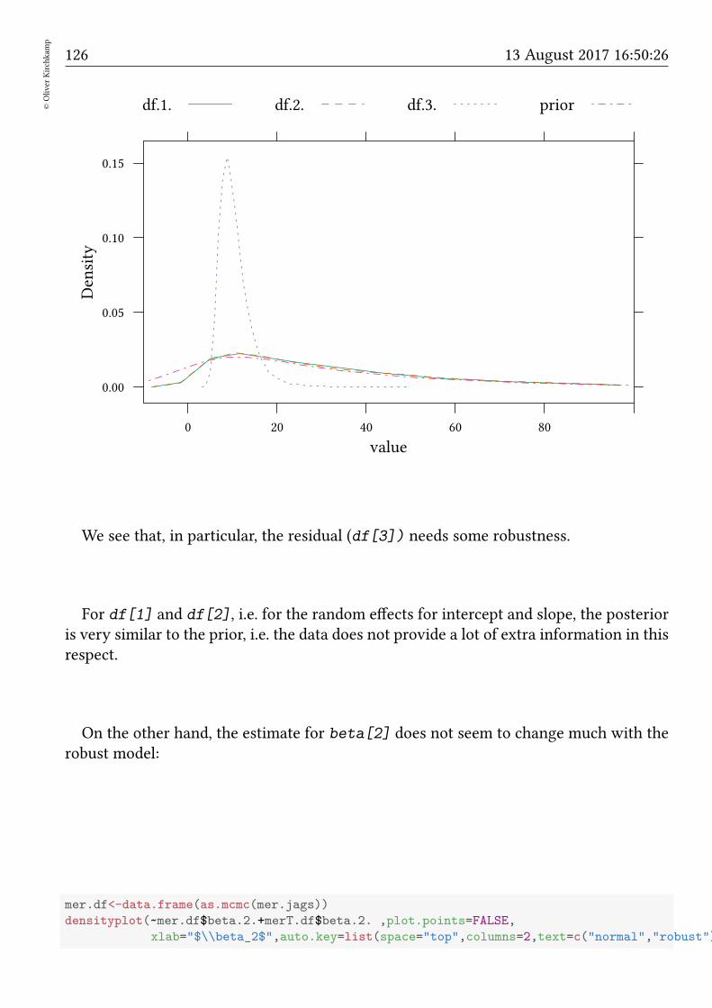
126©Oliver

Kirchkam

p

13 August 2017 16:50:26

value

Density

0.00

0.05

0.10

0.15

0 20 40 60 80

df.1. df.2. df.3. prior

We see that, in particular, the residual (df[3]) needs some robustness.

For df[1] and df[2], i.e. for the random effects for intercept and slope, the posterioris very similar to the prior, i.e. the data does not provide a lot of extra information in thisrespect.

On the other hand, the estimate for beta[2] does not seem to change much with therobust model:

mer.df<-data.frame(as.mcmc(mer.jags))

densityplot(~mer.df$beta.2.+merT.df$beta.2. ,plot.points=FALSE,

xlab="$\\beta_2$",auto.key=list(space="top",columns=2,text=c("normal","robust")))

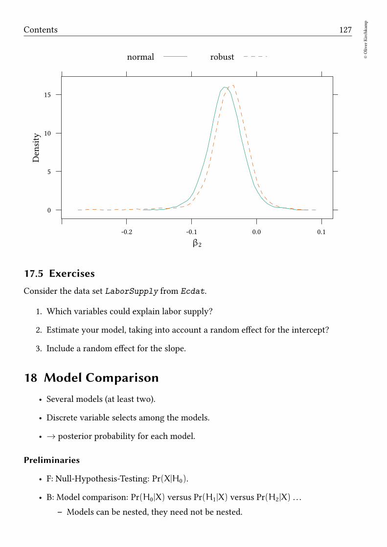
Contents 127

©Oliver

Kirchkam

p

β2

Density

0

5

10

15

-0.2 -0.1 0.0 0.1

normal robust

17.5 Exercises

Consider the data set LaborSupply from Ecdat.

1. Which variables could explain labor supply?

2. Estimate your model, taking into account a random effect for the intercept?

3. Include a random effect for the slope.

18 Model Comparison

• Several models (at least two).

• Discrete variable selects among the models.

• → posterior probability for each model.

Preliminaries

• F: Null-Hypothesis-Testing: Pr(X|H0).

• B: Model comparison: Pr(H0|X) versus Pr(H1|X) versus Pr(H2|X) . . .

– Models can be nested, they need not be nested.

128©Oliver

Kirchkam

p

13 August 2017 16:50:26

– Models can be of different complexity (automatic penalty).

Are these the only plausible models? (similar to a very strong prior)

18.1 Example 1

• Data:

set.seed(123)

x <- rnorm(5,5,1)

• x ∼ N(µ, 1) where N is the normal distribution.

We compare three models:

µ1 = 3.8, µ2 = 4, µ3 = 6.

c.model <- ’model


x[i] ~ dnorm(mu[m],1)

m ~ dcat(modelProb)

’

c.data<-list(x=x,modelProb=c(1,1,1),mu=c(3.8,4,6))

c.jags<-run.jags(c.model,c.data,monitor=c("m"))

with(data.frame(as.mcmc(c.jags)),table(m)/length(m))

m

1 2 3

0.03415 0.12255 0.84330

What is, actually, a vague prior in this context? Can we give more flexibility to theprior for m?

c.model2 <- ’model



m ~ dcat(mP)

mP ~ ddirch(modelProb)

’

c.jags<-run.jags(c.model2,c.data,monitor=c("m"))

with(data.frame(as.mcmc(c.jags)),table(m)/length(m))

m

1 2 3

0.03390 0.12455 0.84155

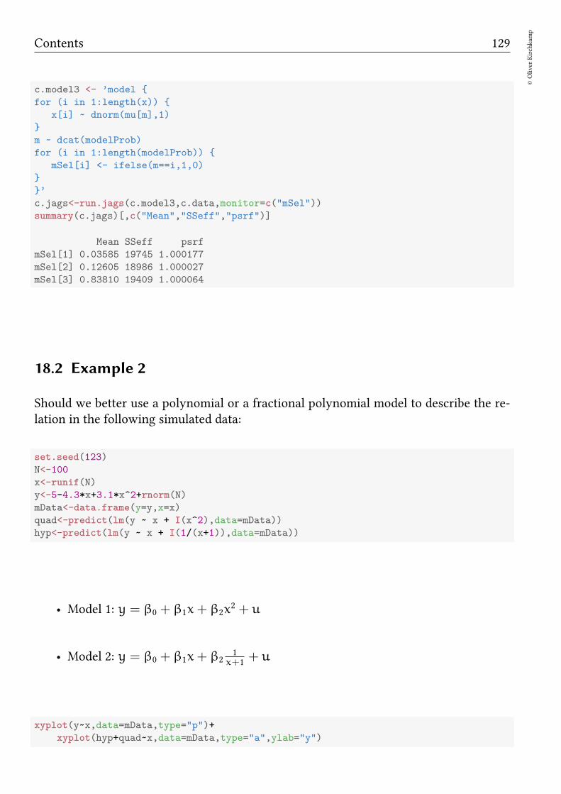
Contents 129

©Oliver

Kirchkam

p

c.model3 <- ’model



m ~ dcat(modelProb)

for (i in 1:length(modelProb))

mSel[i] <- ifelse(m==i,1,0)

’

c.jags<-run.jags(c.model3,c.data,monitor=c("mSel"))

summary(c.jags)[,c("Mean","SSeff","psrf")]

Mean SSeff psrf

mSel[1] 0.03585 19745 1.000177

mSel[2] 0.12605 18986 1.000027

mSel[3] 0.83810 19409 1.000064

18.2 Example 2

Should we better use a polynomial or a fractional polynomial model to describe the re-lation in the following simulated data:

set.seed(123)

N<-100

x<-runif(N)

y<-5-4.3*x+3.1*x^2+rnorm(N)

mData<-data.frame(y=y,x=x)

quad<-predict(lm(y ~ x + I(x^2),data=mData))

hyp<-predict(lm(y ~ x + I(1/(x+1)),data=mData))

• Model 1: y = β0 + β1x+ β2x2 + u

• Model 2: y = β0 + β1x+ β21

x+1+ u

xyplot(y~x,data=mData,type="p")+

xyplot(hyp+quad~x,data=mData,type="a",ylab="y")

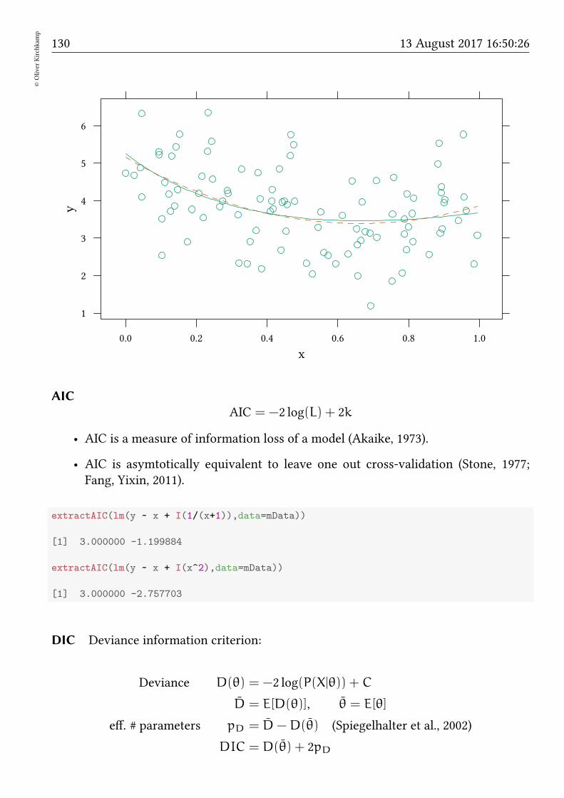
130©Oliver

Kirchkam

p

13 August 2017 16:50:26

x

y

1

2

3

4

5

6

0.0 0.2 0.4 0.6 0.8 1.0

AIC

AIC = −2 log(L) + 2k

• AIC is a measure of information loss of a model (Akaike, 1973).

• AIC is asymtotically equivalent to leave one out cross-validation (Stone, 1977;Fang, Yixin, 2011).

extractAIC(lm(y ~ x + I(1/(x+1)),data=mData))

[1] 3.000000 -1.199884

extractAIC(lm(y ~ x + I(x^2),data=mData))

[1] 3.000000 -2.757703

DIC Deviance information criterion:

Deviance D(θ) = −2 log(P(X|θ)) + C

D = E[D(θ)], θ = E[θ]

eff. # parameters pD = D−D(θ) (Spiegelhalter et al., 2002)

DIC = D(θ) + 2pD

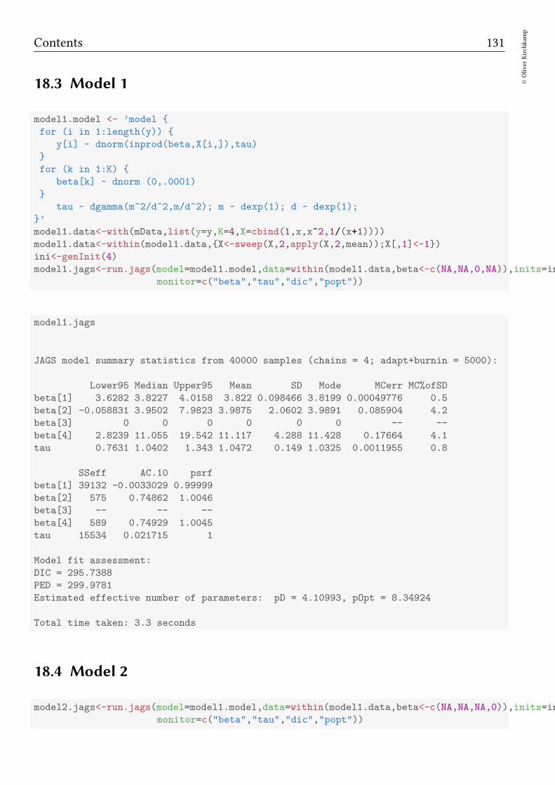
Contents 131

©Oliver

Kirchkam

p

18.3 Model 1

model1.model <- ’model


y[i] ~ dnorm(inprod(beta,X[i,]),tau)

for (k in 1:K)



’

model1.data<-with(mData,list(y=y,K=4,X=cbind(1,x,x^2,1/(x+1))))

model1.data<-within(model1.data,X<-sweep(X,2,apply(X,2,mean));X[,1]<-1)

ini<-genInit(4)

model1.jags<-run.jags(model=model1.model,data=within(model1.data,beta<-c(NA,NA,0,NA)),inits=ini,

monitor=c("beta","tau","dic","popt"))

model1.jags



beta[1] 3.6282 3.8227 4.0158 3.822 0.098466 3.8199 0.00049776 0.5

beta[2] -0.058831 3.9502 7.9823 3.9875 2.0602 3.9891 0.085904 4.2

beta[3] 0 0 0 0 0 0 -- --

beta[4] 2.8239 11.055 19.542 11.117 4.288 11.428 0.17664 4.1

tau 0.7631 1.0402 1.343 1.0472 0.149 1.0325 0.0011955 0.8

SSeff AC.10 psrf

beta[1] 39132 -0.0033029 0.99999

beta[2] 575 0.74862 1.0046

beta[3] -- -- --

beta[4] 589 0.74929 1.0045

tau 15534 0.021715 1

Model fit assessment:

DIC = 295.7388

PED = 299.9781

Estimated effective number of parameters: pD = 4.10993, pOpt = 8.34924


18.4 Model 2

model2.jags<-run.jags(model=model1.model,data=within(model1.data,beta<-c(NA,NA,NA,0)),inits=ini,

monitor=c("beta","tau","dic","popt"))

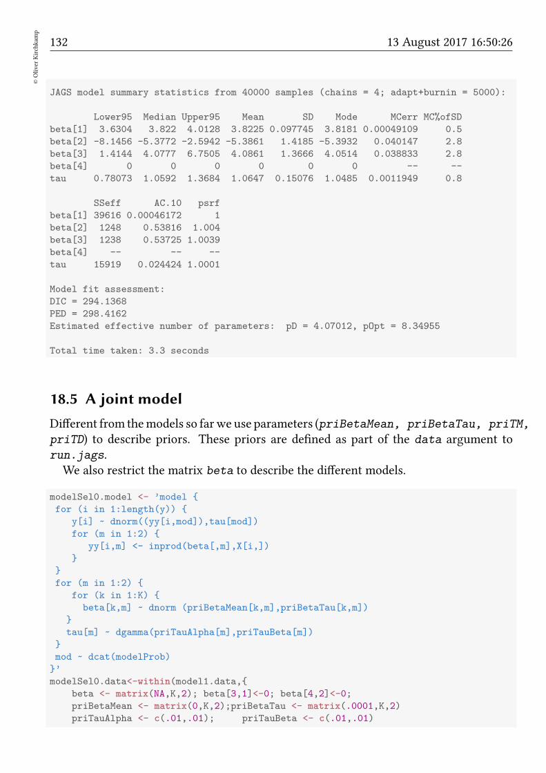
132©Oliver

Kirchkam

p

13 August 2017 16:50:26



beta[1] 3.6304 3.822 4.0128 3.8225 0.097745 3.8181 0.00049109 0.5

beta[2] -8.1456 -5.3772 -2.5942 -5.3861 1.4185 -5.3932 0.040147 2.8

beta[3] 1.4144 4.0777 6.7505 4.0861 1.3666 4.0514 0.038833 2.8

beta[4] 0 0 0 0 0 0 -- --

tau 0.78073 1.0592 1.3684 1.0647 0.15076 1.0485 0.0011949 0.8

SSeff AC.10 psrf

beta[1] 39616 0.00046172 1

beta[2] 1248 0.53816 1.004

beta[3] 1238 0.53725 1.0039

beta[4] -- -- --

tau 15919 0.024424 1.0001

Model fit assessment:

DIC = 294.1368

PED = 298.4162

Estimated effective number of parameters: pD = 4.07012, pOpt = 8.34955


18.5 A joint model

Different from themodels so farwe use parameters (priBetaMean, priBetaTau, priTM,

priTD) to describe priors. These priors are defined as part of the data argument torun.jags.

We also restrict the matrix beta to describe the different models.

modelSel0.model <- ’model


y[i] ~ dnorm((yy[i,mod]),tau[mod])

for (m in 1:2)

yy[i,m] <- inprod(beta[,m],X[i,])

for (m in 1:2)

for (k in 1:K)

beta[k,m] ~ dnorm (priBetaMean[k,m],priBetaTau[k,m])

tau[m] ~ dgamma(priTauAlpha[m],priTauBeta[m])

mod ~ dcat(modelProb)

’

modelSel0.data<-within(model1.data,

beta <- matrix(NA,K,2); beta[3,1]<-0; beta[4,2]<-0;

priBetaMean <- matrix(0,K,2);priBetaTau <- matrix(.0001,K,2)

priTauAlpha <- c(.01,.01); priTauBeta <- c(.01,.01)

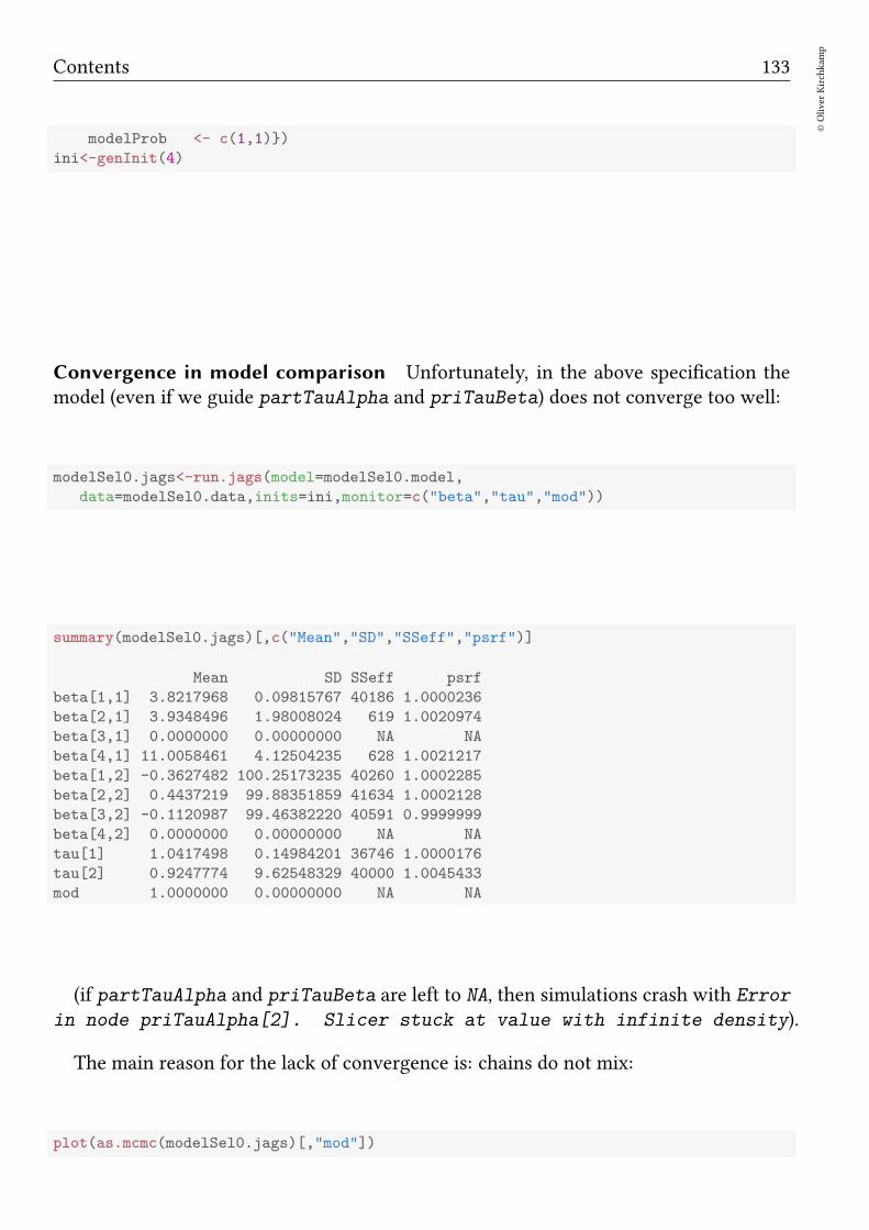
Contents 133

©Oliver

Kirchkam

p

modelProb <- c(1,1))

ini<-genInit(4)

Convergence in model comparison Unfortunately, in the above specification themodel (even if we guide partTauAlpha and priTauBeta) does not converge too well:

modelSel0.jags<-run.jags(model=modelSel0.model,

data=modelSel0.data,inits=ini,monitor=c("beta","tau","mod"))

summary(modelSel0.jags)[,c("Mean","SD","SSeff","psrf")]

Mean SD SSeff psrf

beta[1,1] 3.8217968 0.09815767 40186 1.0000236

beta[2,1] 3.9348496 1.98008024 619 1.0020974

beta[3,1] 0.0000000 0.00000000 NA NA

beta[4,1] 11.0058461 4.12504235 628 1.0021217

beta[1,2] -0.3627482 100.25173235 40260 1.0002285

beta[2,2] 0.4437219 99.88351859 41634 1.0002128

beta[3,2] -0.1120987 99.46382220 40591 0.9999999

beta[4,2] 0.0000000 0.00000000 NA NA

tau[1] 1.0417498 0.14984201 36746 1.0000176

tau[2] 0.9247774 9.62548329 40000 1.0045433

mod 1.0000000 0.00000000 NA NA

(if partTauAlpha and priTauBeta are left to NA, then simulations crash with Error

in node priTauAlpha[2]. Slicer stuck at value with infinite density).

The main reason for the lack of convergence is: chains do not mix:

plot(as.mcmc(modelSel0.jags)[,"mod"])

134©Oliver

Kirchkam

p

13 August 2017 16:50:26

10000 30000

0.6

0.8

1.0

1.2

1.4

Iterations

Trace of var1 Density of var1

01

23

45

0.4 0.6 0.8 1.0 1.2 1.4

What happens if the chain selects one model:

• coefficients for this model adjust.

– likelihood for this model is good.

• coefficients of the other model still follow prior distribution.

– likelihood of the other model is bad.

• → the sampler will almost never switch (model selection is correlated).

Convergence is very slow, we have to help the sampler.

→ Pseudopriors (Carlin, Chib, 1995).

• When model is selected: use vague priors (as before).

• When model is not selected: use pseudopriors (posteriors from previous estima-tion).

modelSel.model <- ’model


y[i] ~ dnorm((yy[i,mod]),tau[mod])

for (m in 1:2) yy[i,m] <- inprod(beta[,m],X[i,])

for (m in 1:2)

for (k in 1:K)

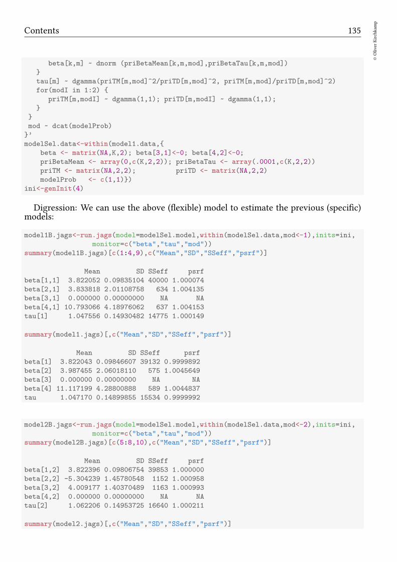
Contents 135

©Oliver

Kirchkam

p

beta[k,m] ~ dnorm (priBetaMean[k,m,mod],priBetaTau[k,m,mod])

tau[m] ~ dgamma(priTM[m,mod]^2/priTD[m,mod]^2, priTM[m,mod]/priTD[m,mod]^2)

for(modI in 1:2)

priTM[m,modI] ~ dgamma(1,1); priTD[m,modI] ~ dgamma(1,1);

mod ~ dcat(modelProb)

’

modelSel.data<-within(model1.data,

beta <- matrix(NA,K,2); beta[3,1]<-0; beta[4,2]<-0;

priBetaMean <- array(0,c(K,2,2)); priBetaTau <- array(.0001,c(K,2,2))

priTM <- matrix(NA,2,2); priTD <- matrix(NA,2,2)

modelProb <- c(1,1))

ini<-genInit(4)

Digression: We can use the above (flexible) model to estimate the previous (specific)models:

model1B.jags<-run.jags(model=modelSel.model,within(modelSel.data,mod<-1),inits=ini,

monitor=c("beta","tau","mod"))

summary(model1B.jags)[c(1:4,9),c("Mean","SD","SSeff","psrf")]

Mean SD SSeff psrf

beta[1,1] 3.822052 0.09835104 40000 1.000074

beta[2,1] 3.833818 2.01108758 634 1.004135

beta[3,1] 0.000000 0.00000000 NA NA

beta[4,1] 10.793066 4.18976062 637 1.004153

tau[1] 1.047556 0.14930482 14775 1.000149

summary(model1.jags)[,c("Mean","SD","SSeff","psrf")]

Mean SD SSeff psrf

beta[1] 3.822043 0.09846607 39132 0.9999892

beta[2] 3.987455 2.06018110 575 1.0045649

beta[3] 0.000000 0.00000000 NA NA

beta[4] 11.117199 4.28800888 589 1.0044837

tau 1.047170 0.14899855 15534 0.9999992

model2B.jags<-run.jags(model=modelSel.model,within(modelSel.data,mod<-2),inits=ini,


summary(model2B.jags)[c(5:8,10),c("Mean","SD","SSeff","psrf")]

Mean SD SSeff psrf

beta[1,2] 3.822396 0.09806754 39853 1.000000

beta[2,2] -5.304239 1.45780548 1152 1.000958

beta[3,2] 4.009177 1.40370489 1163 1.000993

beta[4,2] 0.000000 0.00000000 NA NA

tau[2] 1.062206 0.14953725 16640 1.000211

summary(model2.jags)[,c("Mean","SD","SSeff","psrf")]

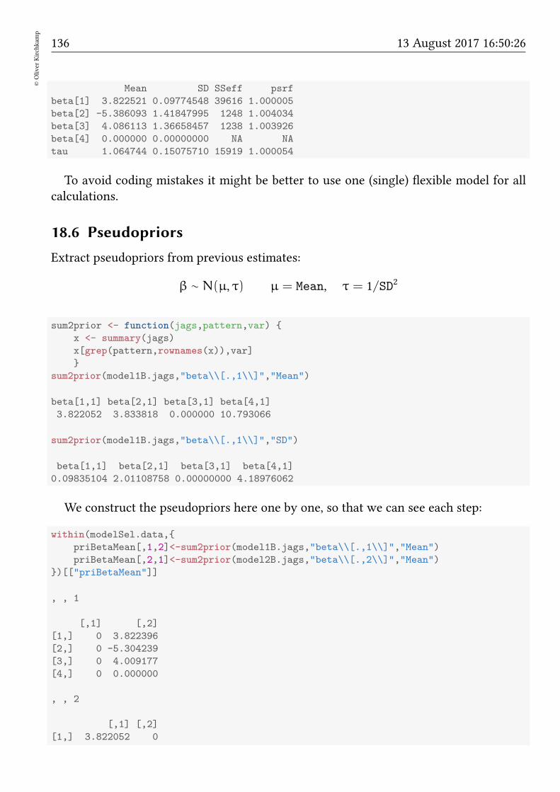
136©Oliver

Kirchkam

p

13 August 2017 16:50:26

Mean SD SSeff psrf

beta[1] 3.822521 0.09774548 39616 1.000005

beta[2] -5.386093 1.41847995 1248 1.004034

beta[3] 4.086113 1.36658457 1238 1.003926

beta[4] 0.000000 0.00000000 NA NA

tau 1.064744 0.15075710 15919 1.000054

To avoid coding mistakes it might be better to use one (single) flexible model for allcalculations.

18.6 Pseudopriors

Extract pseudopriors from previous estimates:

β ∼ N(µ, τ) µ = Mean, τ = 1/SD2

sum2prior <- function(jags,pattern,var)

x <- summary(jags)

x[grep(pattern,rownames(x)),var]

sum2prior(model1B.jags,"beta\\[.,1\\]","Mean")

beta[1,1] beta[2,1] beta[3,1] beta[4,1]

3.822052 3.833818 0.000000 10.793066

sum2prior(model1B.jags,"beta\\[.,1\\]","SD")

beta[1,1] beta[2,1] beta[3,1] beta[4,1]

0.09835104 2.01108758 0.00000000 4.18976062

We construct the pseudopriors here one by one, so that we can see each step:

within(modelSel.data,

priBetaMean[,1,2]<-sum2prior(model1B.jags,"beta\\[.,1\\]","Mean")


)[["priBetaMean"]]

, , 1

[,1] [,2]

[1,] 0 3.822396

[2,] 0 -5.304239

[3,] 0 4.009177

[4,] 0 0.000000

, , 2

[,1] [,2]

[1,] 3.822052 0

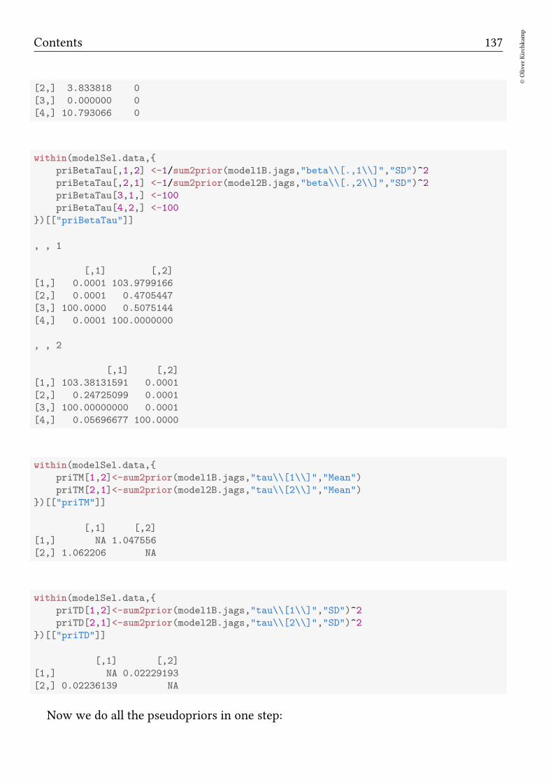
Contents 137

©Oliver

Kirchkam

p

[2,] 3.833818 0

[3,] 0.000000 0

[4,] 10.793066 0


priBetaTau[,1,2] <-1/sum2prior(model1B.jags,"beta\\[.,1\\]","SD")^2


priBetaTau[3,1,] <-100

priBetaTau[4,2,] <-100

)[["priBetaTau"]]

, , 1

[,1] [,2]

[1,] 0.0001 103.9799166

[2,] 0.0001 0.4705447

[3,] 100.0000 0.5075144

[4,] 0.0001 100.0000000

, , 2

[,1] [,2]

[1,] 103.38131591 0.0001

[2,] 0.24725099 0.0001

[3,] 100.00000000 0.0001

[4,] 0.05696677 100.0000


priTM[1,2]<-sum2prior(model1B.jags,"tau\\[1\\]","Mean")


)[["priTM"]]

[,1] [,2]

[1,] NA 1.047556

[2,] 1.062206 NA


priTD[1,2]<-sum2prior(model1B.jags,"tau\\[1\\]","SD")^2


)[["priTD"]]

[,1] [,2]

[1,] NA 0.02229193

[2,] 0.02236139 NA

Now we do all the pseudopriors in one step:

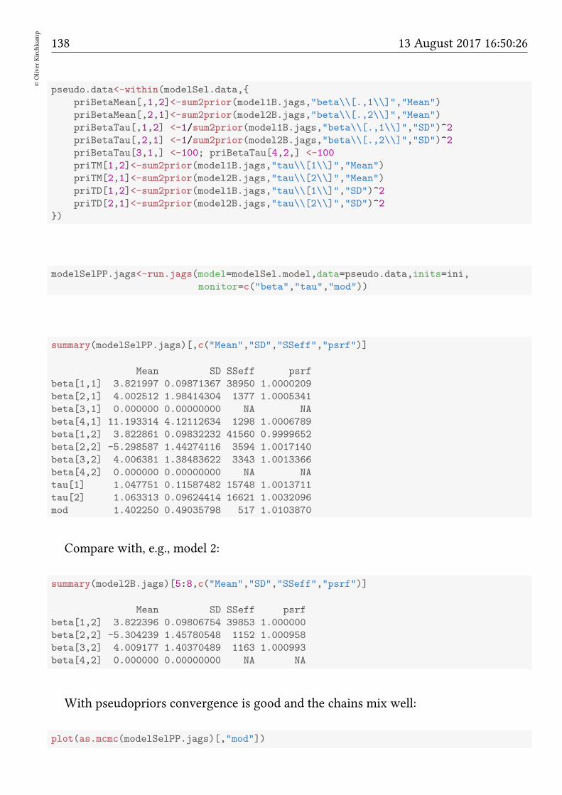
138©Oliver

Kirchkam

p

13 August 2017 16:50:26

pseudo.data<-within(modelSel.data,





priBetaTau[3,1,] <-100; priBetaTau[4,2,] <-100





)

modelSelPP.jags<-run.jags(model=modelSel.model,data=pseudo.data,inits=ini,


summary(modelSelPP.jags)[,c("Mean","SD","SSeff","psrf")]

Mean SD SSeff psrf

beta[1,1] 3.821997 0.09871367 38950 1.0000209

beta[2,1] 4.002512 1.98414304 1377 1.0005341

beta[3,1] 0.000000 0.00000000 NA NA

beta[4,1] 11.193314 4.12112634 1298 1.0006789

beta[1,2] 3.822861 0.09832232 41560 0.9999652

beta[2,2] -5.298587 1.44274116 3594 1.0017140

beta[3,2] 4.006381 1.38483622 3343 1.0013366

beta[4,2] 0.000000 0.00000000 NA NA

tau[1] 1.047751 0.11587482 15748 1.0013711

tau[2] 1.063313 0.09624414 16621 1.0032096

mod 1.402250 0.49035798 517 1.0103870

Compare with, e.g., model 2:

summary(model2B.jags)[5:8,c("Mean","SD","SSeff","psrf")]

Mean SD SSeff psrf

beta[1,2] 3.822396 0.09806754 39853 1.000000

beta[2,2] -5.304239 1.45780548 1152 1.000958

beta[3,2] 4.009177 1.40370489 1163 1.000993

beta[4,2] 0.000000 0.00000000 NA NA

With pseudopriors convergence is good and the chains mix well:

plot(as.mcmc(modelSelPP.jags)[,"mod"])

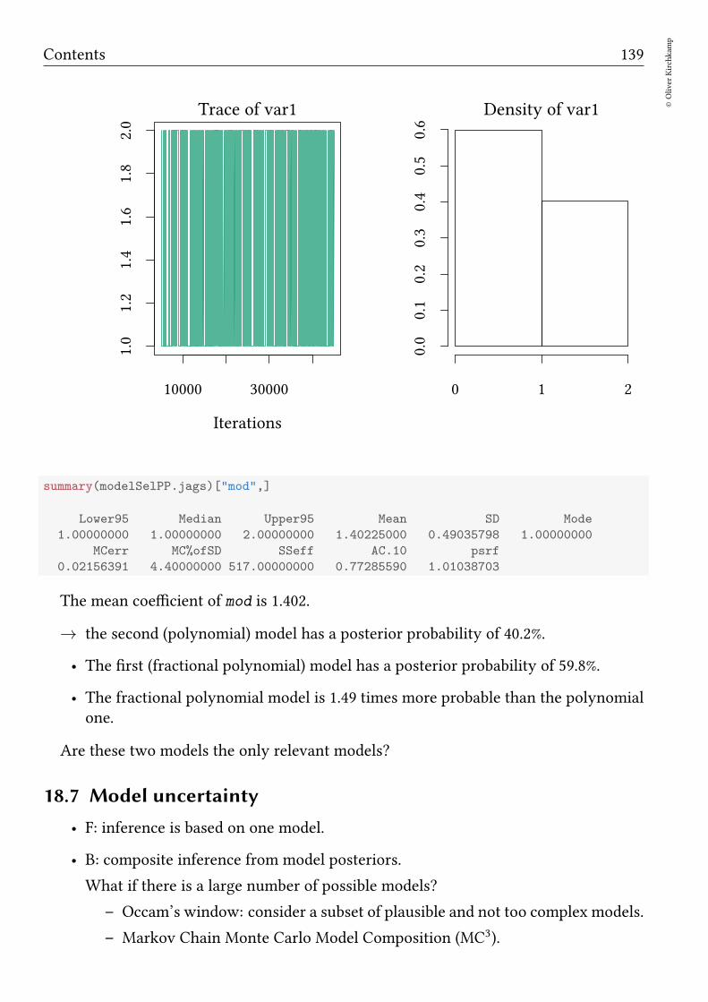
Contents 139

©Oliver

Kirchkam

p

10000 30000

1.0

1.2

1.4

1.6

1.8

2.0

Iterations

Trace of var1 Density of var1

0.0

0.1

0.2

0.3

0.4

0.5

0.6

0 1 2

summary(modelSelPP.jags)["mod",]


1.00000000 1.00000000 2.00000000 1.40225000 0.49035798 1.00000000


0.02156391 4.40000000 517.00000000 0.77285590 1.01038703

The mean coefficient of mod is 1.402.

→ the second (polynomial) model has a posterior probability of 40.2%.

• The first (fractional polynomial) model has a posterior probability of 59.8%.

• The fractional polynomial model is 1.49 times more probable than the polynomialone.

Are these two models the only relevant models?

18.7 Model uncertainty

• F: inference is based on one model.

• B: composite inference from model posteriors.

What if there is a large number of possible models?

– Occam’s window: consider a subset of plausible and not too complex models.

– Markov Chain Monte Carlo Model Composition (MC3).

140©Oliver

Kirchkam

p

13 August 2017 16:50:26

18.8 Bayes factors

Posterior probability of Model H1:

Pr(H1|X) = Pr(H1) · Pr(X|H1)1

Pr(X)

Hence

Pr(H1|X)

Pr(H2|X)=

Pr(H1) · Pr(X|H1)

Pr(H2) · Pr(X|H2)

For uninformed priors Pr(H1) = Pr(H2) we have the Bayes factor

K =Pr(X|H1)

Pr(X|H2)=

∫Pr(θ1|H1) Pr(X|θ1,H1)dθ1∫Pr(θ2|H2) Pr(X|θ2,H2)dθ2

︸︷︷︸Bayes factor

6= Pr(X|θ∗1 ,H1)

Pr(X|θ∗2 ,H2)︸︷︷︸

LR-test

Interpreting K: Harold Jeffreys (1961):

100

barelyworth

mentioning

100.5

substantial

101

strong

101.5

verystrong

102

decisive

Robert E. Kass and Adrian E. Raftery (1995):

e0

barelyworth

mentioning

e1 ≈ 2.7

positive

e3 ≈ 20

strong

e5 ≈ 150

verystrong

19 Mixture Models

19.1 Example

Sometimes we assume that our population can be described as a mixture of two distri-butions. Here we construct such a mixture with means µ = 2 and µ = 3 respectively:

set.seed(123)

N <- 100

group <- rbinom(N,1,.3)

y <- rnorm(N,mean=2+group,sd=.3)

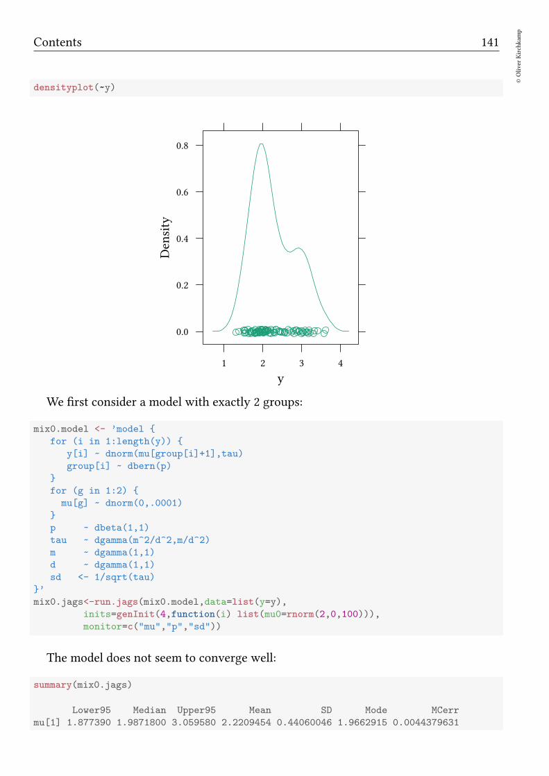
Contents 141

©Oliver

Kirchkam

p

densityplot(~y)

y

Density

0.0

0.2

0.4

0.6

0.8

1 2 3 4

We first consider a model with exactly 2 groups:

mix0.model <- ’model


y[i] ~ dnorm(mu[group[i]+1],tau)

group[i] ~ dbern(p)

for (g in 1:2)

mu[g] ~ dnorm(0,.0001)

p ~ dbeta(1,1)


m ~ dgamma(1,1)

d ~ dgamma(1,1)

sd <- 1/sqrt(tau)

’

mix0.jags<-run.jags(mix0.model,data=list(y=y),

inits=genInit(4,function(i) list(mu0=rnorm(2,0,100))),

monitor=c("mu","p","sd"))

The model does not seem to converge well:

summary(mix0.jags)


mu[1] 1.877390 1.9871800 3.059580 2.2209454 0.44060046 1.9662915 0.0044379631

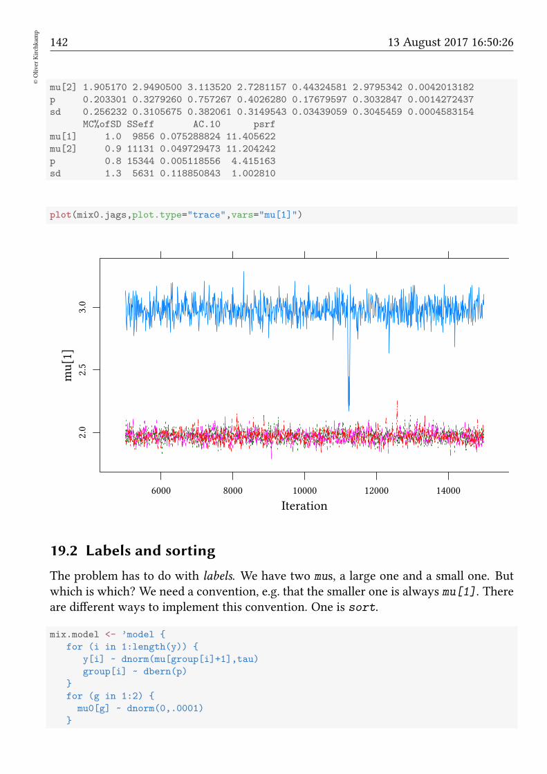
142©Oliver

Kirchkam

p

13 August 2017 16:50:26

mu[2] 1.905170 2.9490500 3.113520 2.7281157 0.44324581 2.9795342 0.0042013182

p 0.203301 0.3279260 0.757267 0.4026280 0.17679597 0.3032847 0.0014272437

sd 0.256232 0.3105675 0.382061 0.3149543 0.03439059 0.3045459 0.0004583154


mu[1] 1.0 9856 0.075288824 11.405622

mu[2] 0.9 11131 0.049729473 11.204242

p 0.8 15344 0.005118556 4.415163

sd 1.3 5631 0.118850843 1.002810

plot(mix0.jags,plot.type="trace",vars="mu[1]")

Iteration

mu[1]

2.0

2.5

3.0

6000 8000 10000 12000 14000

19.2 Labels and sorting

The problem has to do with labels. We have two mus, a large one and a small one. Butwhich is which? We need a convention, e.g. that the smaller one is always mu[1]. Thereare different ways to implement this convention. One is sort.

mix.model <- ’model


y[i] ~ dnorm(mu[group[i]+1],tau)

group[i] ~ dbern(p)

for (g in 1:2)

mu0[g] ~ dnorm(0,.0001)

Contents 143

©Oliver

Kirchkam

p

p ~ dbeta(1,1)

mu[1:2] <- sort(mu0)


m ~ dgamma(1,1)

d ~ dgamma(1,1)

sd <- 1/sqrt(tau)

’

mix.jags<-run.jags(mix.model,data=list(y=y),



summary(mix.jags)


mu[1] 1.876640 1.968230 2.061600 1.9697203 0.04709826 1.9644642 0.0004521677

mu[2] 2.835250 2.981240 3.133600 2.9811188 0.07645630 2.9851922 0.0007250130

p 0.198150 0.303486 0.410794 0.3050988 0.05439289 0.3013208 0.0004569694

sd 0.253974 0.311317 0.382210 0.3156051 0.03377336 0.3048141 0.0004575182


mu[1] 1.0 10850 0.03118628 1.000599

mu[2] 0.9 11121 0.01767753 1.000999

p 0.8 14168 0.01796723 1.000584

sd 1.4 5449 0.10259628 1.000359

19.3 More groups

For a potentially larger number of groups we replace dbern with dcat and dbeta withddirch (the Dirichlet distribution).

mixGen.model <- ’model


y[i] ~ dnorm(mu[group[i]],tau)

group[i] ~ dcat(p)

for (g in 1:G)

mu0[g] ~ dnorm(0,.0001)

alpha[g] <- alphaD # concentration paramter

p[1:G] ~ ddirch(alpha)

mu[1:G] <- sort(mu0)


m ~ dgamma(1,1)

d ~ dgamma(1,1)

sd <- 1/sqrt(tau)

’

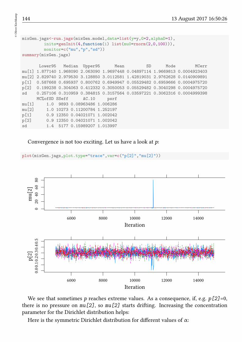
144©Oliver

Kirchkam

p

13 August 2017 16:50:26

mixGen.jags<-run.jags(mixGen.model,data=list(y=y,G=2,alphaD=1),



summary(mixGen.jags)


mu[1] 1.877140 1.968090 2.063090 1.9697448 0.04897114 1.9669813 0.0004923403

mu[2] 2.829740 2.979530 3.128850 3.0112581 1.42819031 2.9762628 0.0140909891

p[1] 0.587668 0.695937 0.800762 0.6949947 0.05529482 0.6959666 0.0004975720

p[2] 0.199238 0.304063 0.412332 0.3050053 0.05529482 0.3040298 0.0004975720

sd 0.257106 0.310959 0.384815 0.3157564 0.03597221 0.3062316 0.0004999398


mu[1] 1.0 9893 0.08963486 1.006286

mu[2] 1.0 10273 0.11200784 1.252197

p[1] 0.9 12350 0.04021071 1.002042

p[2] 0.9 12350 0.04021071 1.002042

sd 1.4 5177 0.15989207 1.013997

Convergence is not too exciting. Let us have a look at p:

plot(mixGen.jags,plot.type="trace",var=c("p[2]","mu[2]"))

Iteration

mu[2]

020

4060

80

6000 8000 10000 12000 14000

Iteration

p[2]

0.00.10.20.30.40.5

6000 8000 10000 12000 14000

We see that sometimes p reaches extreme values. As a consequence, if, e.g. p[2]=0,there is no pressure on mu[2], so mu[2] starts drifting. Increasing the concentrationparameter for the Dirichlet distribution helps:

Here is the symmetric Dirichlet distribution for different values of α:

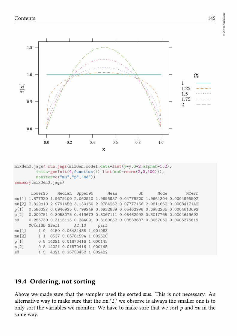
Contents 145

©Oliver

Kirchkam

p

x

f(x)

0.0

0.5

1.0

1.5

0.0 0.2 0.4 0.6 0.8 1.0

α11.251.51.752

mixGen3.jags<-run.jags(mixGen.model,data=list(y=y,G=2,alphaD=1.2),



summary(mixGen3.jags)


mu[1] 1.877330 1.9679100 2.062510 1.9695937 0.04778520 1.9661304 0.0004995502

mu[2] 2.829810 2.9791450 3.130150 2.9784262 0.07777156 2.9811662 0.0008417142

p[1] 0.586327 0.6946925 0.799249 0.6932889 0.05462998 0.6982235 0.0004613692

p[2] 0.200751 0.3053075 0.413673 0.3067111 0.05462998 0.3017765 0.0004613692

sd 0.255730 0.3115115 0.384091 0.3160652 0.03533687 0.3057062 0.0005375619


mu[1] 1.0 9150 0.06431488 1.001063

mu[2] 1.1 8537 0.05781594 1.002620

p[1] 0.8 14021 0.01870416 1.000145

p[2] 0.8 14021 0.01870416 1.000145

sd 1.5 4321 0.16758452 1.002422

19.4 Ordering, not sorting

Above we made sure that the sampler used the sorted mus. This is not necessary. Analternative way to make sure that the mu[1] we observe is always the smaller one is toonly sort the variables we monitor. We have to make sure that we sort p and mu in thesame way.

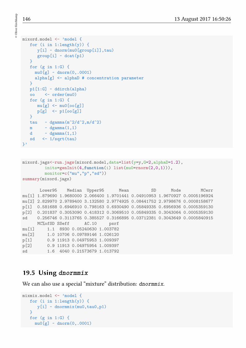
146©Oliver

Kirchkam

p

13 August 2017 16:50:26

mixord.model <- ’model


y[i] ~ dnorm(mu0[group[i]],tau)

group[i] ~ dcat(p1)

for (g in 1:G)

mu0[g] ~ dnorm(0,.0001)

alpha[g] <- alphaD # concentration parameter

p1[1:G] ~ ddirch(alpha)

oo <- order(mu0)

for (g in 1:G)

mu[g] <- mu0[oo[g]]

p[g] <- p1[oo[g]]


m ~ dgamma(1,1)

d ~ dgamma(1,1)

sd <- 1/sqrt(tau)

’

mixord.jags<-run.jags(mixord.model,data=list(y=y,G=2,alphaD=1.2),



summary(mixord.jags)


mu[1] 1.879690 1.9680000 2.066400 1.9701441 0.04910953 1.9670927 0.0005196924

mu[2] 2.829970 2.9789400 3.132580 2.9774925 0.08441752 2.9798676 0.0008158677

p[1] 0.581688 0.6946910 0.798163 0.6930490 0.05849335 0.6956936 0.0005359130

p[2] 0.201837 0.3053090 0.418312 0.3069510 0.05849335 0.3043064 0.0005359130

sd 0.256746 0.3113765 0.385527 0.3166895 0.03712381 0.3043649 0.0005840915


mu[1] 1.1 8930 0.05240630 1.003782

mu[2] 1.0 10706 0.09789146 1.026120

p[1] 0.9 11913 0.04975953 1.009397

p[2] 0.9 11913 0.04975954 1.009397

sd 1.6 4040 0.21573679 1.013792

19.5 Using dnormmix

We can also use a special “mixture” distribution: dnormmix.

mixmix.model <- ’model


y[i] ~ dnormmix(mu0,tau0,p1)

for (g in 1:G)

mu0[g] ~ dnorm(0,.0001)

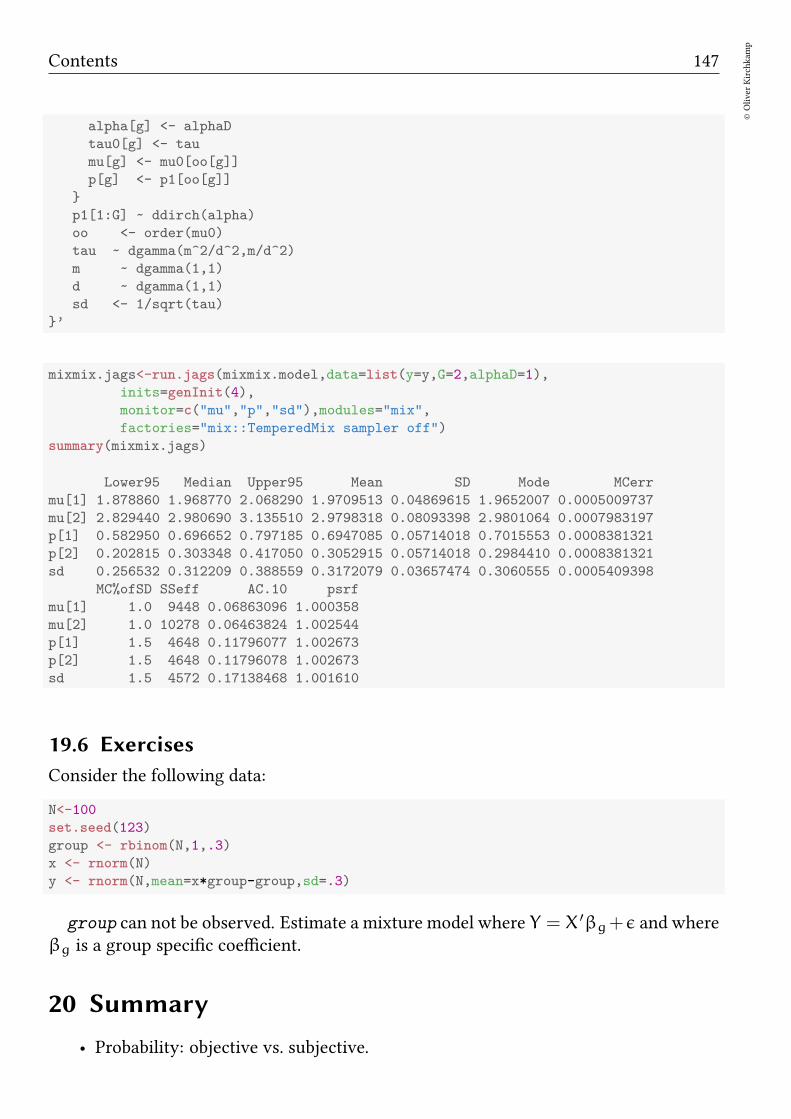
Contents 147

©Oliver

Kirchkam

p

alpha[g] <- alphaD

tau0[g] <- tau

mu[g] <- mu0[oo[g]]

p[g] <- p1[oo[g]]

p1[1:G] ~ ddirch(alpha)

oo <- order(mu0)


m ~ dgamma(1,1)

d ~ dgamma(1,1)

sd <- 1/sqrt(tau)

’

mixmix.jags<-run.jags(mixmix.model,data=list(y=y,G=2,alphaD=1),

inits=genInit(4),

monitor=c("mu","p","sd"),modules="mix",

factories="mix::TemperedMix sampler off")

summary(mixmix.jags)


mu[1] 1.878860 1.968770 2.068290 1.9709513 0.04869615 1.9652007 0.0005009737

mu[2] 2.829440 2.980690 3.135510 2.9798318 0.08093398 2.9801064 0.0007983197

p[1] 0.582950 0.696652 0.797185 0.6947085 0.05714018 0.7015553 0.0008381321

p[2] 0.202815 0.303348 0.417050 0.3052915 0.05714018 0.2984410 0.0008381321

sd 0.256532 0.312209 0.388559 0.3172079 0.03657474 0.3060555 0.0005409398


mu[1] 1.0 9448 0.06863096 1.000358

mu[2] 1.0 10278 0.06463824 1.002544

p[1] 1.5 4648 0.11796077 1.002673

p[2] 1.5 4648 0.11796078 1.002673

sd 1.5 4572 0.17138468 1.001610

19.6 Exercises

Consider the following data:

N<-100

set.seed(123)

group <- rbinom(N,1,.3)

x <- rnorm(N)

y <- rnorm(N,mean=x*group-group,sd=.3)

group can not be observed. Estimate a mixture model where Y = X ′βg+ǫ and whereβg is a group specific coefficient.

20 Summary

• Probability: objective vs. subjective.

148©Oliver

Kirchkam

p

13 August 2017 16:50:26

• Priors, how to get them?

• Results: F: depend on intention of the experimenter

B: depend on prior.

• Flexible modelling: F. has only a limited number of models.

F: precise models which are sometimes not such a good representation of the prob-lem.

B: approximate models which can be a more precise representation of the problem.

• Interpretation: p-values versus posteriors.

B. predicts (posterior) probability of a hypothesis.

F. writes carefully worded statements which are wrong 5% of the time (or any otherprobability) provided H0 is true.

• Quality of decisions: p-values are only a heuristics for a decision rule.

B.’s decisions are better in expectation.

21 Exercises

Exercise 21.1 You assume that X ∼ N(µ, τ).

Your prior is µ ∼ N(10, 1), τ = 2.

Your sample is X = 8, 9, 10.

What is your posterior for µ and τ?

Exercise 21.2 (Female labour supply) Have a look at the dataset Mroz in Ecdat. Esti-

mate the following model

hoursw = β0 + β1educw + β2income + ǫi

Compare two specifications:

• First assume that hoursw is not censored. Use standard OLS and a Bayesian specifi-

cation.

• Then assume that hoursw is censored at zero. Use a standard ML model and a

Bayesian specification.

• Next make this a robust regression, taking into account the censoring.

Exercise 21.3 (Young males) Have a look at the dataset Males in Ecdat.

Contents 149

©Oliver

Kirchkam

p

1. Estimate amixed effectsmodel that explains wage as a function of exper and school.

Include a random effect on the intercept for the identity of the male. Use Maximum

Likelihood and a Bayesian Model. Check convergence.

2. Use a robust model.

Bayes - Summer 2017 - Kirchkamp · Contents 5 © Oliver Kirchkamp 1 Introduction 1.1 Preliminaries...

Documents

Transcript of Bayes - Summer 2017 - Kirchkamp · Contents 5 © Oliver Kirchkamp 1 Introduction 1.1 Preliminaries...