Aster Models for Life History Analysis

by CHARLES J. GEYER

School of Statistics, University of Minnesota, 313 Ford Hall, 224 Church Street S. E.,

Minneapolis, Minnesota 55455, U. S. A.

charlie@stat.umn.edu

STUART WAGENIUS

Institute for Plant Conservation Biology, Chicago Botanic Garden, 1000 Lake Cook Road,

Glencoe, Illinois 60022, U. S. A.

wagenius@chicagobotanic.org

and RUTH G. SHAW

Department of Ecology, Evolution, and Behavior, University of Minnesota, 100 Ecology

Building, 1987 Upper Buford Circle, St. Paul, Minnesota 55108, U. S. A.

rshaw@superb.ecology.umn.edu

Summary

We present a new class of statistical models, designed for life history analysis of plants

and animals, that allow joint analysis of data on survival and reproduction over multiple

years, allow for variables having different probability distributions, and correctly account for

the dependence of variables on earlier variables. We illustrate their utility with an analysis

of data taken from an experimental study of Echinacea angustifolia sampled from remnant

prairie populations in western Minnesota. These models generalise both generalised linear

models and survival analysis. The joint distribution is factorised as a product of conditional

1

distributions, each an exponential family with the conditioning variable being the sample

size of the conditional distribution. The model may be heterogeneous, each conditional

distribution being from a different exponential family. We show that the joint distribution

is from a flat exponential family and derive its canonical parameters, Fisher information

and other properties. These models are implemented in an R package ‘aster’ available from

the Comprehensive R Archive Network, CRAN.

Some key words: Conditional exponential family; Flat exponential family; Generalised

linear model; Graphical model; Maximum likelihood.

1. Introduction

This article introduces a class of statistical models we call ‘aster models’. They were

invented for life history analysis of plants and animals and are best introduced by an example

about perennial plants observed over several years. For each individual planted, at each

census, we record whether or not it is alive, whether or not it flowers, and its number of

flower heads. These data are complicated, especially when recorded for several years, but

simple conditional models may suffice. We consider mortality status, dead or alive, to be

Bernoulli given the preceding mortality status. Similarly, flowering status given mortality

status is also Bernoulli. Given flowering, the number of flower heads may have a zero-

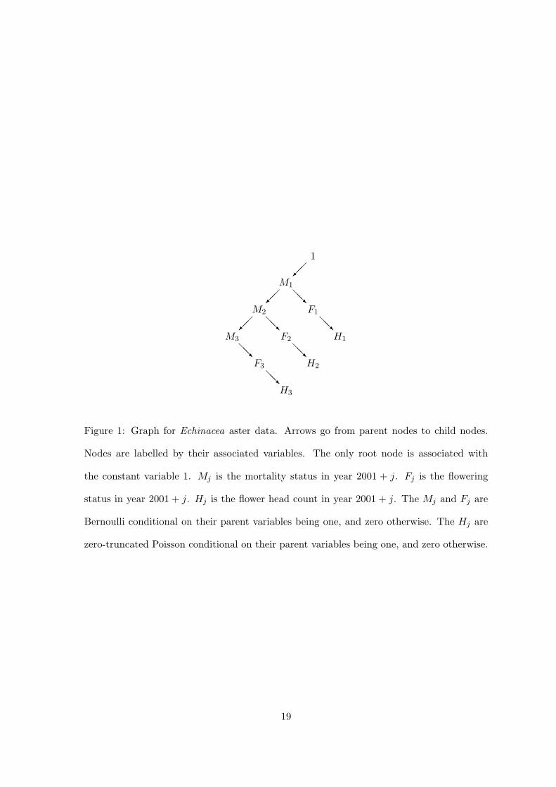
truncated Poisson distribution (Martin, et al., 2005). Figure 1 shows the graphical model

for a single individual.

[Figure 1 about here.]

This aster model generalises both discrete time Cox regression (Cox, 1972; Breslow, 1972,

1974) and generalised linear models (McCullagh & Nelder, 1989). Aster models apply to

any similar conditional modelling. We could, for example, add other variables, such as seed

count modelled conditional on flower head count.

2

A simultaneous analysis that models the joint distribution of all the variables in a life

history analysis can answer questions that cannot be addressed through separate analyses

of each variable conditional on the others. Joint analysis also deals with structural zeros

in the data; for example, a dead individual remains dead and cannot flower, so in Fig. 1

any arrow that leads from a variable that is zero to another variable implies that the

other variable must also be zero. Such zeros present intractable missing data problems in

separate analyses of individual variables. Aster models have no problem with structural

zeros; likelihood inference automatically handles them correctly.

Aster models are simple graphical models (Lauritzen, 1996, § 3.2.3) in which the joint

density is a product of conditionals as in equation (1) below. No knowledge of graphical

model theory is needed to understand aster models. One innovative aspect of aster models

is the interplay between two parameterisations described in §§ 2·2 and 2·3 below. The

‘conditional canonical parameterisation’ arises when each conditional distribution in the

product is an exponential family and we use the canonical parameterisation for each. The

‘unconditional canonical parameterisation’ arises from observing that the joint model is a full

flat exponential family (Barndorff-Nielsen, 1978, Ch. 8) and using the canonical parameters

for that family, defined by equation (5) below.

2. Aster Models

2·1. Factorisation and graphical model

Variables in an aster model are denoted byXj , where j runs over the nodes of a graph. A

general aster model is a chain graph model (Lauritzen, 1996, pp. 7, 53) having both arrows,

corresponding to directed edges, and lines, corresponding to undirected edges. Figure 1

is special, having only arrows. Arrows go from parent to child, lines between neighbours.

Nodes that are not children are called root nodes. Those that are not parents are called

3

terminal nodes.

Let F and J denote root and non-root nodes. Aster models have very special chain

graph structure determined by a partition G of J and a function p : G → J ∪ F . For each

G ∈ G there is an arrow from p(G) to each element of G and a line between each pair of

elements of G. For any set S, let XS denote the vector whose components are Xj , j ∈ S.

The graph determines a factorisation

pr(XJ |XF ) =∏

G∈G

pr{XG|Xp(G)}; (1)

compare equation 3.23 in Lauritzen (1996).

Elements of G are called chain components because they are connectivity components of

the chain graph (Lauritzen, 1996, pp. 6–7). Since Fig. 1 has no undirected edge, each node

is a chain component by itself. Allowing nontrivial chain components allows the elements

of XG to be conditionally dependent given Xp(G) with merely notational changes to the

theory. In our example in § 5 the graph consists of many copies of Fig. 1, one for each

individual plant. Individuals have no explicit representation. For any set S, let p−1(S)

denote the set of G such that p(G) ∈ S. Then each subgraph consisting of one G ∈ p−1(F ),

its descendants, children, children of children, etc., and arrows and lines connecting them,

corresponds to one individual. If we make each such G have a distinct root element p(G),

then the set of descendants of each root node corresponds to one individual. Although all

individuals in our example have the same subgraph, this is not required.

2·2. Conditional exponential families

We take each of the conditional distributions in (1) to be an exponential family having

canonical statistic XG that is the sum of Xp(G) independent and identically distributed

random vectors, possibly a different such family for each G. Conditionally, Xp(G) = 0

implies that XG = 0G almost surely. If j 6= p(G) for any G, then the values of Xj are

4

unrestricted. If the distribution of XG given Xp(G) is infinitely divisible, such as Poisson or

normal, for each G ∈ p−1({j}), then Xj must be nonnegative and real-valued. Otherwise,

Xj must be nonnegative and integer-valued.

The loglikelihood for the whole family has the form

∑

G∈G

∑

j∈G

Xjθj −Xp(G)ψG(θG)

=

∑

j∈J

Xjθj −∑

G∈G

Xp(G)ψG(θG), (2)

where θG is the canonical parameter vector for the Gth conditional family, having compo-

nents θj , j ∈ G, and ψG is the cumulant function for that family (Barndorff-Nielsen, 1978,

pp. 105, 139, 150) that satisfies

EθG{XG|Xp(G)} = Xp(G)∇ψG(θG) (3)

varθG{XG|Xp(G)} = Xp(G)∇

2ψG(θG), (4)

where varθ(X) is the variance-covariance matrix of X and ∇2ψ(θ) is the matrix of second

partial derivatives of ψ (Barndorff-Nielsen, 1978, p. 150).

2·3. Unconditional exponential families

Collecting terms with the same Xj in (2), we obtain

∑

j∈J

Xj

θj −

∑

G∈p−1({j})

ψG(θG)

−

∑

G∈p−1(F )

Xp(G)ψG(θG)

and see that

ϕj = θj −∑

G∈p−1({j})

ψG(θG), j ∈ J, (5)

are the canonical parameters of an unconditional exponential family with canonical statistics

Xj . We now write X instead of XJ , ϕ instead of ϕJ , and so forth, and let 〈X,ϕ〉 denote the

inner product∑

j Xjϕj . Then we can write the loglikelihood of this unconditional family

as

l(ϕ) = 〈X,ϕ〉 − ψ(ϕ), (6)

5

where the cumulant function of this family is

ψ(ϕ) =∑

G∈p−1(F )

Xp(G)ψG(θG). (7)

All of the Xp(G) in (7) are at root nodes, and hence are nonrandom, so that ψ is a determin-

istic function. Also the right-hand side of (7) is a function of ϕ by the logic of exponential

families (Barndorff-Nielsen, 1978, pp. 105 ff.).

The system of equations (5) can be solved for the θj in terms of the ϕj in one pass

through the equations in any order that finds θj for children before parents. Thus (5)

determines an invertible change of parameter.

2·4. Canonical affine models

One of the desirable aspects of exponential family canonical parameter affine models

defined by reparameterisation of the form

ϕ = a+Mβ, (8)

where a is a known vector, called the origin, and M is a known matrix, called the model

matrix, is that, because 〈X,Mβ〉 = 〈MTX,β〉, the result is a new exponential family with

canonical statistic

Y = MTX (9)

and canonical parameter β. The dimension of this new family will be the dimension of β,

if M has full rank.

As is well known (Barndorff-Nielsen, 1978, p. 111), the canonical statistic of an ex-

ponential family is minimal sufficient. Since we have both conditional and unconditional

families in play, we stress that this well-known result is about unconditional families. A

dimension reduction to a low-dimensional sufficient statistic like (9) does not occur when

the conditional canonical parameters θ are modelled affinely, and this suggests that affine

6

models for the unconditional parameterisation may be scientifically more interesting despite

their more complicated structure.

2·5. Mean-value parameters

Conditional mean values

ξj = EθG{Xj |Xp(G)} = Xp(G)

∂ψG(θG)

∂θj, j ∈ G, (10)

are not parameters because they contain random data Xp(G), although they play the role of

mean-value parameters when we condition on Xp(G), treating it as constant. By standard

exponential family theory (Barndorff-Nielsen, 1978, p. 121), ∇ψG is an invertible change of

parameter.

Unconditional mean-value parameters are the unconditional expectations

τ = Eϕ{X} = ∇ψ(ϕ). (11)

By standard theory, ∇ψ : ϕ 7→ τ is an invertible change of parameter. The unconditional

expectation in (11) can be calculated using the iterated expectation theorem

Eϕ{Xj} = Eϕ{Xp(G)}∂ψG(θG)

∂θj, j ∈ G, (12)

where θ is determined from ϕ by solving (5). The system of equations (12) can produce the

τj in one pass through the equations in any order that finds τj for parents before children.

3. Likelihood Inference

3·1. Conditional models

The score ∇l(θ) for conditional canonical parameters is particularly simple, having com-

ponents

∂l(θ)

∂θj= Xj −Xp(G)

ψG(θG)

∂θj, j ∈ G, (13)

7

and, if these parameters are modelled affinely as in (8) but with ϕ replaced by θ, then

∇l(β) = ∇l(θ)M. (14)

The observed Fisher information matrix for θ, which is the matrix −∇2l(θ), is block

diagonal with

−∂2l(θ)

∂θi∂θj= Xp(G)

∂2ψG(θG)

∂θi∂θj, i, j ∈ G, (15)

the only nonzero entries. The expected Fisher information matrix for θ is the unconditional

expectation of the observed Fisher information matrix, calculated using (15) and (12).

If I(θ) denotes either the observed or the expected Fisher information matrix for θ and

similarly for other parameters, then

I(β) = MT I(θ)M. (16)

3·2. Unconditional models

The score ∇l(ϕ) for unconditional canonical parameters is, as in every unconditional

exponential family, ‘observed minus expected’:

∂l(ϕ)

∂ϕj= Xj − Eϕ{Xj},

the unconditional expectation on the right-hand side being evaluated by using (12). If these

parameters are modelled affinely as in (8), then we have (14) with θ replaced by ϕ. Note

that (13) is not ‘observed minus conditionally expected’ if considered as a vector equation

because the conditioning would differ amongst components.

Second derivatives with respect to unconditional canonical parameters of an exponential

family are nonrandom, and hence observed and expected Fisher information matrices I(ϕ)

are equal, given by either of the expressions ∇2ψ(ϕ) and varϕ(X). Fix θ and ϕ related by

(5). For i, j ∈ G, the iterated covariance formula gives

covϕ{Xi, Xj} =∂2ψG(θG)

∂θi∂θjEϕ

{Xp(G)

}+∂ψG(θG)

∂θi

∂ψG(θG)

∂θjvarϕ

{Xp(G)

}. (17)

8

Otherwise we may assume that j ∈ G and i is not a descendant of j so that

covϕ{Xi, Xj |Xp(G)} = 0 because Xj is conditionally independent given Xp(G) of all variables

except itself and its descendants. Then the iterated covariance formula gives

covϕ{Xi, Xj} =∂ψG(θG)

∂θjcovϕ

{Xi, Xp(G)

}. (18)

Expectations having been calculated using (12), variances, the case i = j in (17), are

calculated in one pass through (17) in any order that deals with parents before children.

Then another pass using (17) and (18) gives covariances. The information matrix for β is

given by (16) with θ replaced by ϕ.

3·3. Prediction

By ‘prediction’, we only mean evaluation of a function of estimated parameters, what

the predict function in R does for generalised linear models. In aster models we have five

different parameterisations of interest, β, θ, ϕ, ξ and τ . The Fisher information matrix

for β, already described, handles predictions of β, so this section is about ‘predicting’ the

remaining four.

One often predicts for new individuals having different covariate values from the observed

individuals. Then the model matrix M̃ used for the prediction is different from that used

for calculating β̂ and the Fisher information matrix I(β̂), either observed or expected.

Let η be the affine predictor, i. e., η = θ for conditional models and η = ϕ for uncon-

ditional models, let ζ be any one of θ, ϕ, ξ and τ , and let f : η 7→ ζ. Suppose we wish to

predict

g(β) = h(ζ) = h{f(M̃β)

}. (19)

Then, by the chain rule, (19) has derivative

∇g(β) = ∇h(ζ)∇f(η)M̃, (20)

9

and, by the ‘usual’ asymptotics of maximum likelihood and the delta method, the asymp-

totic distribution of the prediction h(ζ̂) = g(β̂) is

N[g(β), {∇g(β̂)}I(β̂)−1{∇g(β̂)}T

],

where ∇g(β̂) is given by (20) with η̂ = M̃β̂ plugged in for η and ζ̂ = f(η̂) plugged in for ζ.

We write ‘predictions’ in this complicated form to separate the parts of the specification, the

functions h and ∇h and the model matrix M̃ , that change from application to application

from the part ∇f that does not change and can be dealt with by computer; see Appendix A

of the technical report at http://www.stat.umn.edu/geyer/aster for details.

To predict mean-value parameters one must specify new ‘response’ data Xj as well

as new ‘covariate’ data in M̃ . Unconditional mean-value parameters τ depend on Xj ,

j ∈ F , whereas conditional mean-value parameters ξ depend on Xj , j ∈ J ∪ F . It is often

interesting, however, to predict ξ for hypothetical individuals with Xj = 1 for all j, thus

obtaining conditional mean values per unit sample size.

4. Software

We have released an R (R Development Core Team, 2004) package aster that fits,

tests, predicts and simulates aster models. It uses the R formula mini-language, originally

developed for genstat and S (Wilkinson & Rogers, 1973; Chambers & Hastie, 1992) so

that model fitting is much like that for linear or generalised linear models. The R function

summary.aster provides regression coefficients with standard errors, z statistics and p-

values; anova.aster provides likelihood ratio tests for model comparison; predict.aster

provides the predictions with standard errors described in § 3·3; raster generates random

aster model data for simulation studies or parametric bootstrap calculations. The package

is available from CRAN (http://www.cran.r-project.org) and is open source.

The current version of the package limits the general model described in this article

10

in several ways. In predictions, only linear h are allowed in (19), but this can be worked

around. For general h, observe that h(ζ̂) and AT ζ̂, where A = ∇h(ζ), have the same

standard errors. Thus, obtain h(ζ̂) by one call to predict.aster and the standard errors

for AT ζ̂, where A = ∇h(ζ̂) by a second call. In models, the only conditional families

currently implemented are Bernoulli, Poisson, k-truncated Poisson, negative binomial and

k-truncated negative binomial, but adding another one-parameter exponential family would

require only implementation of its ψ, ψ′ and ψ′′ functions and its random variate generator.

Multiparameter conditional families, chain components, are not yet implemented. Allowing

terminal nodes that are two-parameter normal or allowing child nodes that are multinomial

given a common parent would require more extensive changes to the package.

5. Example

Data were collected on 570 individuals of Echinacea angustifolia, each having the data

structure shown in Fig. 1. These plants were sampled as seeds from seven remnant pop-

ulations that are surviving fragments of the tall-grass prairie that a century ago covered

western Minnesota and other parts of the Great Plains of North America. The plants were

experimentally randomised at the time of planting into a field within 6.5 km of all pop-

ulations of origin. The dataset contains three predictor variables: ewloc and nsloc give

east-west and north-south positions of individuals and pop gives their remnant population

of origin. To use the R formula mini-language we need to create more variables: resp is a

vector comprising the response variables, the Mj , Fj and Hj ; level is categorical naming

the type of response variable, with values M , F and H; year is categorical giving the year;

varb is the interaction of level and year; and hdct is short for level = H.

We fitted many models; see Appendix D of the technical report at http://www.stat.

umn.edu/geyer/aster for details. Scientific interest focuses on the model comparison

11

shown in Table 1.

[Table 1 about here.]

The models are nested. The affine predictor for Model 4 can be written

ϕj = µLj ,Yj+ αLj

Uj + βLjVj + γLj ,Pj

, (21)

where Lj , Yj , Uj , Vj and Pj are level, year, ewloc, nsloc and pop, respectively, and the

alphas, betas and gammas are regression coefficients. Model 3 is the submodel of Model 4

that imposes the constraint γM,P = γF,P , for all populations P . Model 2 is the submodel of

Model 3 that imposes the constraint γM,P = γF,P = 0, for all P . Model 1 is the submodel

of Model 2 that imposes the constraint γL,P = 0, for all L and P .

All models contain the graph node effect, varb or µLj ,Yj, and the quantitative spatial

effect, level:(nsloc + ewloc) or αLjUj + βLj

Vj , which was chosen by comparing many

models; for details see the technical report. We explain here only differences amongst

models, which involve only categorical predictors. In an unconditional aster model, which

these are, such terms require the maximum likelihood estimates of mean-value parameters

for each category, summed over all individuals in the category, to match their observed

values: ‘observed equals expected’. Model 4 makes observed equal expected for total head

count∑

j Hj , for total flowering∑

j Fj , and for total survival∑

j Mj within each population.

Model 3 makes observed equal expected for total head count∑

j Hj and for total non-head

count∑

j(Mj + Fj) within each population. Model 2 makes observed equal expected for

total head count∑

j Hj within each population.

From purely statistical considerations, Model 3 is the best of these four nested models.

Model 4 does not fit significantly better. Model 2 fits significantly worse. It is difficult

to interpret Model 3 scientifically, because ‘non-head count’∑

j(Mj + Fj) is unnatural, in

effect scoring 0 for dead, 1 for alive without flowers or 2 for alive with flowers.

12

Model 2 is the model of primary scientific interest. Evolutionary biologists are funda-

mentally interested in fitness, but it is notoriously diffcult to measure; see Beatty (1992),

Keller (1992) and Paul (1992). The fitness of an individual may be defined as its lifetime

contribution of progeny to the next generation. For these data the most direct surrogate

measure for fitness is total head count∑

j Hj . The currently available data represent a

small fraction of this plant’s lifespan. To obtain more complete measures of fitness, we are

continuing these experiments and collecting these data for successive years.

Biologists call all our measured variables, the Mj , Fj and Hj , ‘components of fitness’.

Since Mj and Fj contribute to fitness only through Hj , in an aster model the unconditional

expectation of Hj , its unconditional mean-value parameter, completely accounts for the

contributions of Mj and Fj . Strictly speaking, this is not quite true, since we do not have

Hj measured over the whole life span, so the last Mj contains the information about future

reproduction, but it becomes more true as more data are collected in future years. Moreover,

we have no data about life span and do not wish to inject subjective opinion about future

flower head count into the analysis.

The statistical point of this is that the Mj and Fj are in the model only to produce

the correct stochastic structure. If we could directly model the marginal distribution of the

Hj , but we cannot, we would not need the other variables. They are ‘nuisance variables’

that must be in the model but are of no interest in this particular analysis; the mean-value

parameters for those variables are nuisance parameters. Model 3 is the best according to

the likelihood ratio test, but does it fit the variables of interest better than Model 2? We

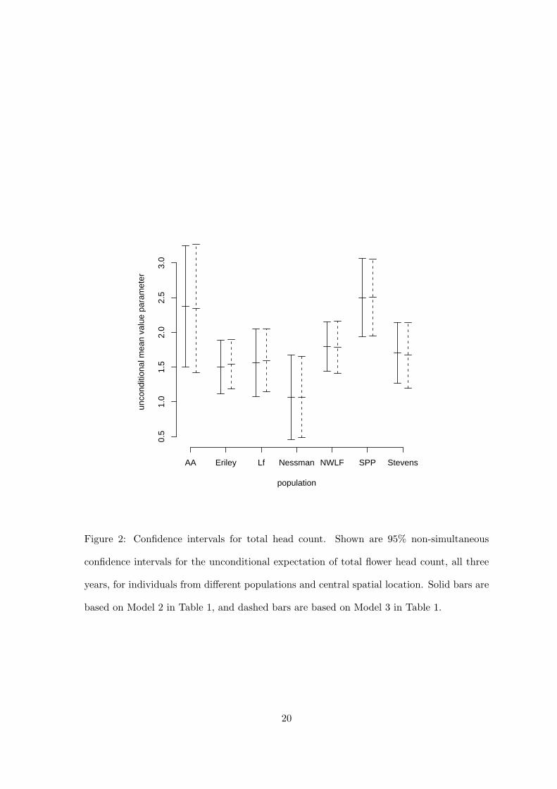
do not know of an established methodology for addressing this issue, so we propose looking

at confidence intervals for the mean-value parameters for total flower head count shown in

Fig. 2.

[Figure 2 about here.]

13

Although we have no formal test to propose, we claim that it is obvious that Model 3 is no

better than Model 2 at ‘predicting’ the best surrogate of expected fitness. We take this as

justification for using Model 2 in scientific discussion and infer from it significant differences

among the populations in flower head count and, thus, fitness.

It being difficult to interpret Model 3 scientifically, Model 4 is the next larger readily

interpretable model. Model 4 does fit significantly better than Model 2, P = 0.00016,

which implies differences among populations in mortality and flowering (the Mj and Fj)

that may be of scientific interest even though they make no direct contribution to fitness,

since Model 2 already fully accounts for their contributions through Hj .

Note that we would have obtained very different results had we used a conditional

model, not shown, see § D.3.2 of the technical report. The parameters of interest are

unconditional expectations of total flower head count. This alone suggests an unconditional

model. Furthermore, we see in (5) that unconditional aster models ‘mix levels’ passing

information up from children to parents. This is why Model 2 in our example was successful

in predicting total head count while only modelling pop effects at head count nodes. Since

a conditional aster model does not mix levels in this way, it must model all levels and so

usually needs many more parameters than an unconditional model.

6. Discussion

The key idea of aster models, as we see it, is the usefulness of what we have called uncon-

ditional aster models, which have low-dimensional sufficient statistics (9). Following Geyer

& Thompson (1992), who argued in favour of exponential family models with sufficient

statistics chosen to be scientifically interpretable, an idea they attributed to Jaynes (1978),

we emphasise the value of these models in analyses of life histories and overall fitness.

We do not insist, however, the R package aster is even-handed with respect to condi-

14

tional and unconditional models and conditional and unconditional parameters. Users may

use whatever seems best to them. Any joint analysis is better than any separate analyses

of different variables. We have, however, one warning. In an unconditional aster model, as

in all exponential family models, the map from canonical parameters to mean-value param-

eters is monotone; with sufficient statistic vector Y given by (9) having components Yk we

have

−∂2l(β)

∂β2k

=∂Eβ{Yk}

∂βk

> 0. (22)

This gives regression coefficients their simple interpretation: an increase in βk causes an

increase in Eβ{Yk}, other betas being held constant. The analogue of (22) for a conditional

model is

−∂2l(β)

∂β2k

=∂

∂βk

∑

G∈G

∑

j∈G

Eβ{Xj |Xp(G)}mjk > 0, (23)

where mjk are components ofM . Because we cannot move the sums in (23) inside the condi-

tional expectation, there is no corresponding simple interpretation of regression coefficients.

Conditional aster models are therefore algebraically simple but statistically complicated.

Unconditional aster models are algebraically complicated but statistically simple. They

can be simply explained as flat exponential families having the desired sufficient statistics.

They are the aster models that behave according to the intuitions derived from linear and

generalised linear models.

We saw in our example that aster models allowed us to model fitness successfully. In

medical applications, Darwinian fitness is rarely interesting, but aster models may allow data

on mortality or survival to be analyzed in combination with other data, such as quality of

life measures.

15

Acknowledgements

Our key equation (5) was derived about 1980 when R. G. S. was a graduate student

and C. J. G. not yet a graduate student. R. G. S.’s Ph. D. adviser Janis Antonovics

provided some funding for development, from a now forgotten source, but which we thank

nevertheless. High quality life history data, generated recently by S. W., Julie Etterson,

David Heiser and Stacey Halpern, and work of Helen Hangelbroek, supported by the U. S.

National Science Foundation, about what in hindsight we would call a conditional aster

model analysis of mortality data, motivated implementation of these ideas. Were it not for

Janis’s enthusiastic encouragement back then, we might not have been able to do this now.

We should also acknowledge the R team. Without R we would never have made software as

usable and powerful as the aster package. We also thank Robert Gentleman for pointing

out the medical implications.

References

Barndorff-Nielsen, O. E. (1978). Information and Exponential Families. Chichester:

John Wiley.

Beatty, J. (1992). Fitness: Theoretical contexts. In Keywords in Evolutionary Biology,

Ed. E. F. Keller and E. A. Lloyd, pp. 115–9. Cambridge, MA: Harvard University Press.

Breslow, N. (1972). Discussion of the paper by Cox (1972). J. R. Statist. Soc. B 34,

216–7.

Breslow, N. (1974). Covariance analysis of censored survival data. Biometrics, 30, 89-99.

Chambers, J. M. & Hastie, T. J. (1992). Statistical models. In Statistical Models in

S, Ed. J. M. Chambers and T. J. Hastie, pp. 13–44. Pacific Grove, CA: Wadsworth &

Brooks/Cole.

16

Cox, D. R. (1972). Regression models and life-tables (with Discussion). J. R. Statist. Soc.

B 34, 187–220.

Geyer, C. J. & Thompson, E. A. (1992). Constrained Monte Carlo maximum likelihood

for dependent data (with Discussion). J. R. Statist. Soc. B 54 657–99.

Jaynes, E. T. (1978). Where do we stand on maximum entropy? In The Maximum

Entropy Formalism, Ed. R. D. Levine and M. Tribus, pp. 15-118. Cambridge, MA: MIT

Press.

Keller, E. F. (1992). Fitness: Reproductive ambiguities. In Keywords in Evolutionary

Biology, Ed. E. F. Keller and E. A. Lloyd, pp. 120–1. Cambridge, MA: Harvard University

Press.

Lauritzen, S. L. (1996). Graphical Models. New York: Oxford University Press.

Martin, T. G., Wintle, B. A., Rhodes, J. R., Kuhnert, P. M., Field, S. A.,

Low-Choy, S. J., Tyre, A. J. & Possingham, H. P. (2005). Zero tolerance ecology:

improving ecological inference by modelling the source of zero observations. Ecol. Lett. 8

1235–46.

McCullagh, P. & Nelder, J. A. (1989). Generalized Linear Models, 2nd ed. London:

Chapman and Hall.

Paul, D. (1992). Fitness: Historical perspective. In Keywords in Evolutionary Biology,

Ed. E. F. Keller and E. A. Lloyd, pp. 112–4. Cambridge, MA: Harvard University Press.

R Development Core Team (2004). R: A language and environment for statistical

computing. R Foundation for Statistical Computing, Vienna, Austria. http://www.

R-project.org.

17

Wilkinson, G. N. & Rogers, C. E. (1973). Symbolic description of factorial models for

analysis of variance. Appl. Statist. 22, 392–9.

18

1

M1

M2

M3

F1

F2

F3

H1

H2

H3

��

��

��

@@R

@@R@@R

@@R@@R

@@R

Figure 1: Graph for Echinacea aster data. Arrows go from parent nodes to child nodes.

Nodes are labelled by their associated variables. The only root node is associated with

the constant variable 1. Mj is the mortality status in year 2001 + j. Fj is the flowering

status in year 2001 + j. Hj is the flower head count in year 2001 + j. The Mj and Fj are

Bernoulli conditional on their parent variables being one, and zero otherwise. The Hj are

zero-truncated Poisson conditional on their parent variables being one, and zero otherwise.

19

0.5

1.0

1.5

2.0

2.5

3.0

unco

nditi

onal

mea

n va

lue

para

met

er

AA Eriley Lf Nessman NWLF SPP Stevens

population

Figure 2: Confidence intervals for total head count. Shown are 95% non-simultaneous

confidence intervals for the unconditional expectation of total flower head count, all three

years, for individuals from different populations and central spatial location. Solid bars are

based on Model 2 in Table 1, and dashed bars are based on Model 3 in Table 1.

20

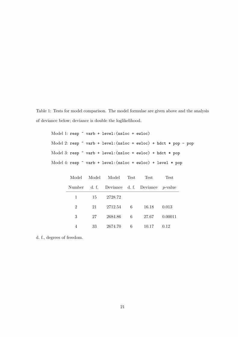
Table 1: Tests for model comparison. The model formulae are given above and the analysis

of deviance below; deviance is double the loglikelihood.

Model 1: resp ~ varb + level:(nsloc + ewloc)

Model 2: resp ~ varb + level:(nsloc + ewloc) + hdct * pop - pop

Model 3: resp ~ varb + level:(nsloc + ewloc) + hdct * pop

Model 4: resp ~ varb + level:(nsloc + ewloc) + level * pop

Model Model Model Test Test Test

Number d. f. Deviance d. f. Deviance p-value

1 15 2728.72

2 21 2712.54 6 16.18 0.013

3 27 2684.86 6 27.67 0.00011

4 33 2674.70 6 10.17 0.12

d. f., degrees of freedom.

21