arX

iv:a

stro

-ph/

9708

202v

1 2

2 A

ug 1

997

KSUPT-97/1, KUNS-1448 May 1997

MAX 4 and MAX 5 CMB anisotropy measurement constraints on

open and flat-Λ CDM cosmogonies

Ken Ganga1, Bharat Ratra2, Mark A. Lim3, Naoshi Sugiyama4, and Stacy T. Tanaka5

Received ; accepted

1IPAC, MS 100–22, California Institute of Technology, Pasadena, CA 91125.

2Department of Physics, Kansas State University, Manhattan, KS 66506.

3Department of Physics, University of California, Santa Barbara, CA 93106.

4Department of Physics, Kyoto University, Kitashirakawa-Oiwakecho, Sakyo-ku, Kyoto 606.

5Department of Physics, University of California, Berkeley, CA 94720.

– 2 –

ABSTRACT

We account for experimental and observational uncertainties in likelihood analyses

of cosmic microwave background (CMB) anisotropy data from the MAX 4 and MAX

5 experiments. These analyses use CMB anisotropy spectra predicted in open and

spatially-flat Λ cold dark matter cosmogonies. Amongst the models considered,

the combined MAX data set is most consistent with the CMB anisotropy shape in

Ω0 ∼ 0.1− 0.2 open models and less so with that in old (t0>∼

15 − 16 Gyr, i.e., low h),

high baryon density (ΩB>∼

0.0175h−2), low density (Ω0 ∼ 0.2 − 0.4), flat-Λ models.

The MAX data alone do not rule out any of the models we consider at the 2σ level.

Model normalizations deduced from the combined MAX data are consistent with

those drawn from the UCSB South Pole 1994 data, except for the flat bandpower model

where MAX favours a higher normalization. The combined MAX data normalization

for open models with Ω0 ∼ 0.1 − 0.2 is higher than the upper 2σ value of the

DMR normalization. The combined MAX data normalization for old (low h), high

baryon density, low-density flat-Λ models is below the lower 2σ value of the DMR

normalization. Open models with Ω0 ∼ 0.4 − 0.5 are not far from the shape most

favoured by the MAX data, and for these models the MAX and DMR normalizations

overlap. The MAX and DMR normalizations also overlap for Ω0 = 1 and some higher

h, lower ΩB, low-density flat-Λ models.

Subject headings: cosmic microwave background — cosmology: observations —

large-scale structure of the universe

– 3 –

1. Introduction

Recent measurements of spatial anisotropy in the cosmic microwave background indicate

that CMB anisotropy data will soon provide useful constraints on cosmological parameters such

as Ω0, h, and ΩB (Bennett et al. 1996; Ganga et al. 1994; Gutierrez et al. 1997; Piccirillo et

al. 1997; Netterfield et al. 1997; Gundersen et al. 1995; Tucker at al. 1997; Platt et al. 1997;

Masi et al. 1996; Lim et al. 1996, hereafter L96; Cheng et al. 1997; Griffin et al. 1997; Scott et

al. 1996; Leitch et al. 1997; Church et al. 1997, see Page 1997 for a review). Here, the present

value of the (total) nonrelativistic-mass density parameter Ω0, is 8πGρb(t0)/(3H02), where G is

the gravitational constant, ρb(t0) is the mean nonrelativistic-mass density now, H0 = 100h km s−1

Mpc−1 is the Hubble parameter now, and ΩB is the current value of the baryonic-mass density

parameter.

Ganga et al. (1997a, hereafter GRGS) developed general methods to account for experimental

and observational uncertainties, such as beamwidth and calibration uncertainties, in likelihood

analysis of CMB data sets. These methods have previously been used in conjunction with

theoretically-predicted CMB anisotropy spectra in analyses of the Gundersen et al. (1995) SP94

data and the Church et al. (1997) SuZIE data (GRGS; Ganga et al. 1997b). Bond & Jaffe (1997)

have also analyzed the SP94 data and the Netterfield et al. (1997) SK data.

In this paper we present results from a similar analysis of the MAX 4 and MAX 5 CMB

anisotropy data sets (Devlin et al. 1994; Clapp et al. 1994; Tanaka et al. 1996, hereafter T96;

L96). MAX 4 and MAX 5 are the most recent of the published balloon-borne MAX CMB

anisotropy experiments. The original MAX detector and the MAX 1 results are discussed in

Fischer et al. (1992). The ACME telescope used in these MAX experiments is described in

Meinhold et al. (1993a). The MAX 2 observational results are in Alsop et al. (1992). Meinhold

et al. (1993b) and Gundersen et al. (1993) present the MAX 3 results. Analyses of the MAX 3

observations, in the context of the fiducial CDM model, is given in Srednicki et al. (1993) and

Dodelson & Stebbins (1994).

– 4 –

Descriptions of MAX 4 and 5 are given in Devlin et al. (1994), Clapp et al. (1994), T96, and

L96; we review here the information needed for our analyses. Data were taken in four frequency

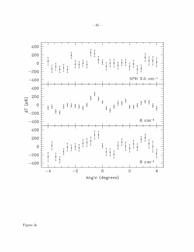
bands centered at 3.5, 6, 9, and 14 cm−1; our analyses do not use the 14 cm−1 band data. The

FWHM of the beams, assumed to be gaussian, are: 0.55 ± 0.05 for the MAX 4 3.5 cm−1 band,

0.75 ± 0.05 for the MAX 4 6/9 cm−1 bands, 0.5(1 ± 0.10) for the MAX 5 3.5 cm−1 band,

and 0.55(1 ± 0.10) for the MAX 5 6/9 cm−1 bands, where the uncertainties are one standard

deviation. The MAX data used here were taken during smooth, constant velocity, constant

declination, azimuthal scans extending 6 on the sky for MAX 4 and 8 on the sky for MAX 5.

While observing, the beam was sinusoidally chopped with a half peak-to-peak amplitude of 1.4

on the sky. The data were coadded into 21 bins for MAX 4 and 29 bins for MAX 5.

MAX 4 data were taken in smooth scans of ±3 on the sky centered near the stars γ Ursae

Minoris, ι Draconis (hereafter 4ID), and σ Herculis (hereafter 4SH). Sky rotation has a significant

effect on the γ Ursae Minoris scan pattern (Devlin et al. 1994), so we do not analyze this data

set here. The bin positions in the released 4ID and 4SH data sets are data-weighted averages (A.

Clapp, private communication 1996); we use evenly spaced bins in this analysis. MAX 5 data

were taken in smooth scans of ±4 on the sky centered near the stars HR5127 (hereafter 5HR),

µ Pegasi (hereafter 5MP), and φ Herculis (hereafter 5PH). The 9 cm−1 5PH data is thought to

contain atmospheric emission (T96, 5PH data was taken at lower balloon altitude), and is not

used for CMB anisotropy analyses. The 5MP data has structure that correlates with IRAS 100

µm dust emission (L96). Off-diagonal noise correlations affect the 5HR and 5PH results by <∼2%

(T96), and are ignored here.

MAX 4 and 5 were calibrated primarily by using a membrane transfer standard (Fischer et

al. 1992); the absolute calibration uncertainty is 10% (1σ).

In §2 we summarize some of the computational techniques used in our analysis. Our results

and a discussion are in §3, and we conclude in §4.

– 5 –

2. Summary of Computation

Our conventions, notation, and techniques are those of GRGS.

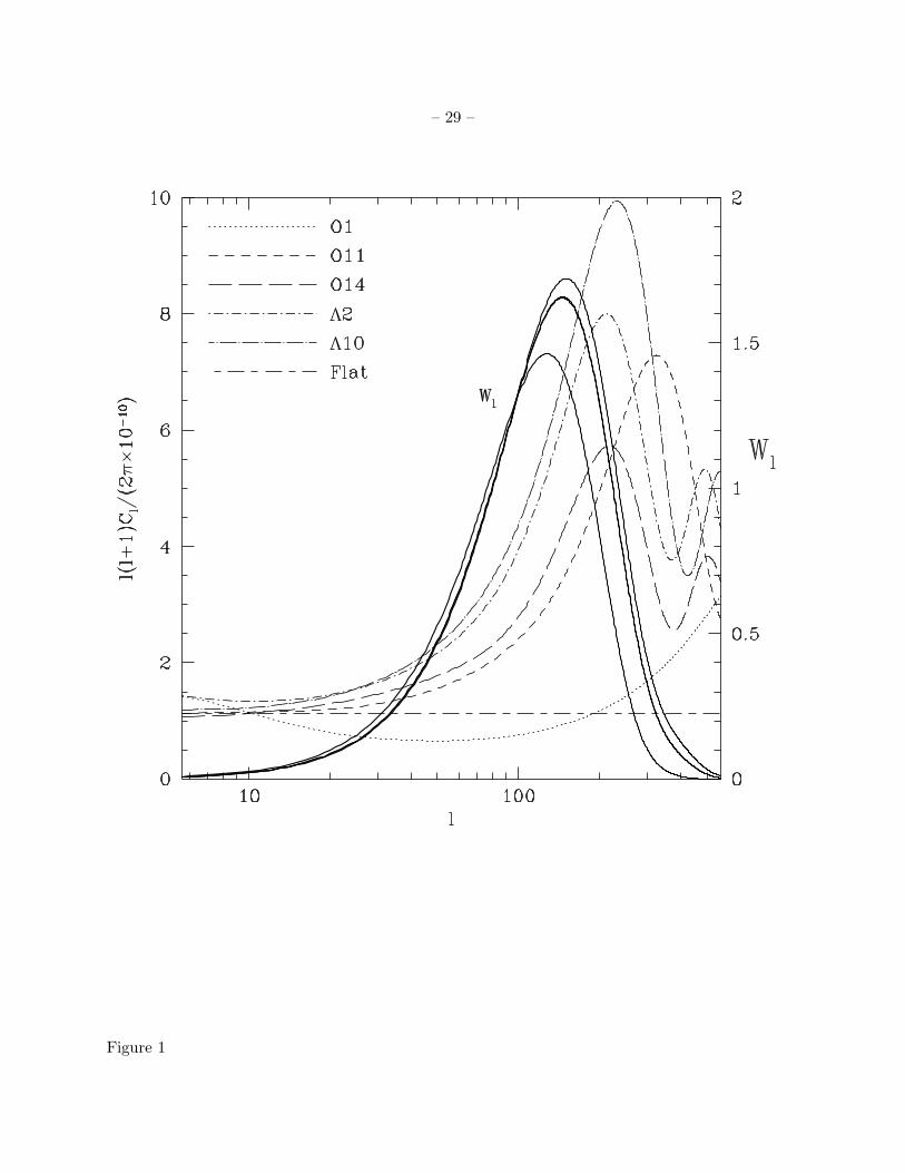
The CMB anisotropy spectra for some of the models we consider here are shown in Figure 1.

The models are described in Ratra et al. (1997) and GRGS, and the computation of the spectra

is discussed in Sugiyama (1995). Besides the flat bandpower and fiducial CDM models, we also

consider open and flat-Λ CDM cosmogonies. The models assume gaussian, adiabatic, primordial

energy-density power spectra. The flat-Λ models assume a scale-invariant energy-density power

spectrum (Harrison 1970; Peebles & Yu 1970; Zel’dovich 1972), as is found in the simplest

spatially-flat inflation models (Guth 1981, also see Kazanas 1980; Sato 1981a,b). The open models

assume the energy-density power spectrum (Ratra & Peebles 1994, 1995; Bucher, Goldhaber, &

Turok 1995; Yamamoto, Sasaki, & Tanaka 1995) of the simplest open-bubble inflation models (Gott

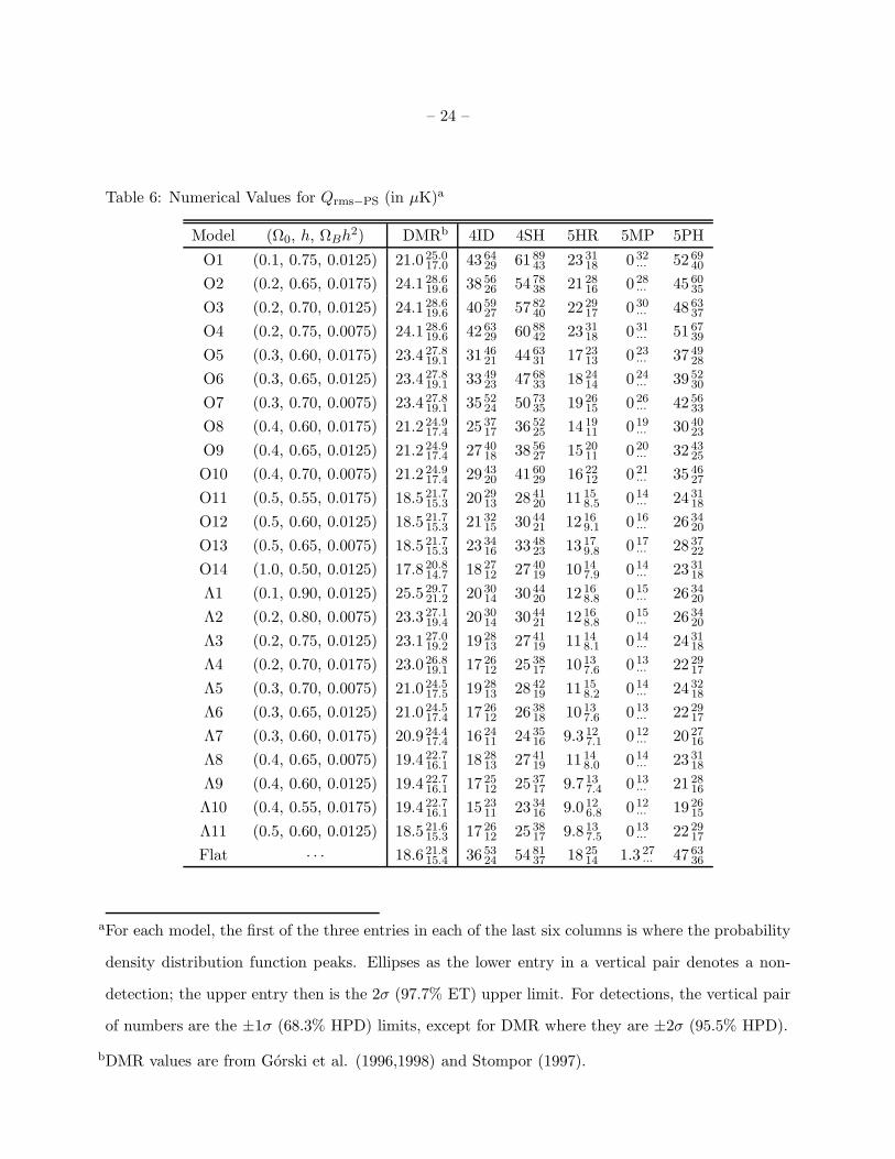
1982; Guth & Weinberg 1983). The model spectra are parameterized by the quadrupole-moment

amplitude of the CMB anisotropy, Qrms−PS, as well as Ω0, h, and ΩB. The spectra shown in

Figure 1 are normalized to the DMR maps (Gorski et al. 1996,1998; Stompor 1997). Parameter

values for the models considered are given in Table 6.

The low-density models considered here are the simplest ones roughly consistent with most

current observations. For flat-Λ models see Kitayama & Suto (1996), Ratra et al. (1997), Bunn

& White (1997), Turner (1997), Peacock (1997), and Cole et al. (1997), and for the open case see

Kitayama & Suto (1996), Ratra et al. (1997), Gorski et al (1998), Gott (1997), Peacock (1997),

and Cole et al. (1997). The values of the parameters Ω0, h, and ΩB used here are chosen to be

roughly consistent with present observational estimates of Ω0, h, the age of the universe, and the

constraints on ΩB that follow from standard nucleosynthesis (Ratra et al. 1997). In this analysis

we ignore the effects of tilt, primordial gravity waves, and reionization. These effects are unlikely

to be significant in viable open models.6 In order to reconcile some of the flat-Λ models with

6 Maia & Lima (1996), Tanaka & Sasaki (1997), and Bucher & Cohn (1997) have studied

primordial gravity waves in the open model. Initial indications are that predictions based on

– 6 –

observational data, however, some such effect is needed to suppress intermediate-scale (CMB and

matter) and small-scale (matter) power (Stompor, Gorski, & Banday 1995; Ostriker & Steinhardt

1995; Ratra et al. 1997; Klypin, Primack, & Holtzman 1996; Ganga, Ratra, & Sugiyama 1996;

Maddox, Efstathiou, & Sutherland 1996; Peacock 1997; Cole et al. 1997).

Figure 1 also shows the four different zero-lag window functions, Wl, for the individual MAX

channels at their nominal beamwidths. The usual window function parameters, the value of l

where Wl is largest, lm, the two values of l where Wle−0.5

= e−0.5Wlm , le−0.5 , and the effective

multipole, le, are given in Table 1 for these window functions (e.g., Bond 1996; GRGS).

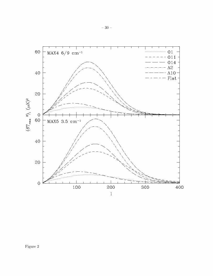
Figure 2 shows the moments (δTrms2)l for two MAX window functions and some selected

CMB anisotropy spectra (GRGS, eqs. [5] & [6]). Given an assumed CMB anisotropy spectrum,

these moments provide a convenient measure of the range of l to which MAX is sensitive.

Table 2 gives lm, the value of l at which (δTrms2)l is largest, and le−0.5 the two multipoles where

(δTrms2)l

e−0.5

= e−0.5(δTrms2)lm , for the MAX window functions and the models we consider. As

is true for SP94 and SuZIE, the range of multipole moments to which each window function is

sensitive is quite model dependent (GRGS; Ganga et al. 1997b).

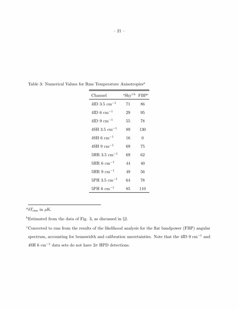
The reduced MAX 4 and MAX 5 data are shown in Figure 3. In Table 3, the column labelled

“Sky” indicates the estimated anisotropy rms for those individual channel data sets thought to be

purely CMB anisotropy. This is computed from the data of Figure 3 as the square root of the

difference between the variance of the mean temperatures and the variance of the error bars.

The computation of the likelihood function is described in GRGS. The only difference between

what is done here and in GRGS is that for the 5MP data (but not the other data sets) we also

marginalized over a possible dust contamination given by the spectrum in L96 and an arbitrary

spatial morphology. Beamwidth and calibration uncertainties are accounted for as described

in GRGS. We again use three-point Gauss-Hermite quadrature to marginalize over beamwidth

the simplest observationally-viable single-scalar-field open-bubble-inflation energy-density power

spectrum (Ratra & Peebles 1994, 1995) are negligibly affected by primordial gravity waves.

– 7 –

uncertainty.

In Table 3, the column labelled “FBP” lists central δTrms values derived from likelihood

analyses using the flat bandpower (FBP) spectrum.

To derive the Qrms−PS central value and limits from the likelihood function we assume a

uniform prior in Qrms−PS(≥ 0). The central value is taken to be the value of Qrms−PS at which

the probability density distribution peaks. The MAX limits we quote are ±1σ highest posterior

density (HPD) limits for (2σ HPD) detections. For nondetections we quote upper 2σ equal tail

(ET) limits.7

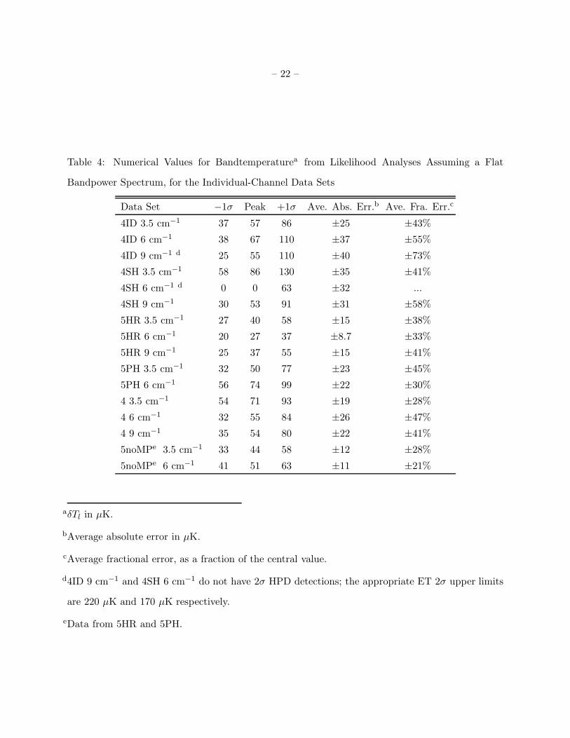
In Table 4 we give bandtemperature (δTl = δTrms/ [∑

∞

l=2 [(l + 0.5)Wl/l(l + 1)]]0.5, e.g.,

Bond 1996; GRGS, eq. [7]) central values and ±1σ limits derived from flat bandpower likelihood

analyses of the individual-channel MAX data sets. The last two columns give the average of the

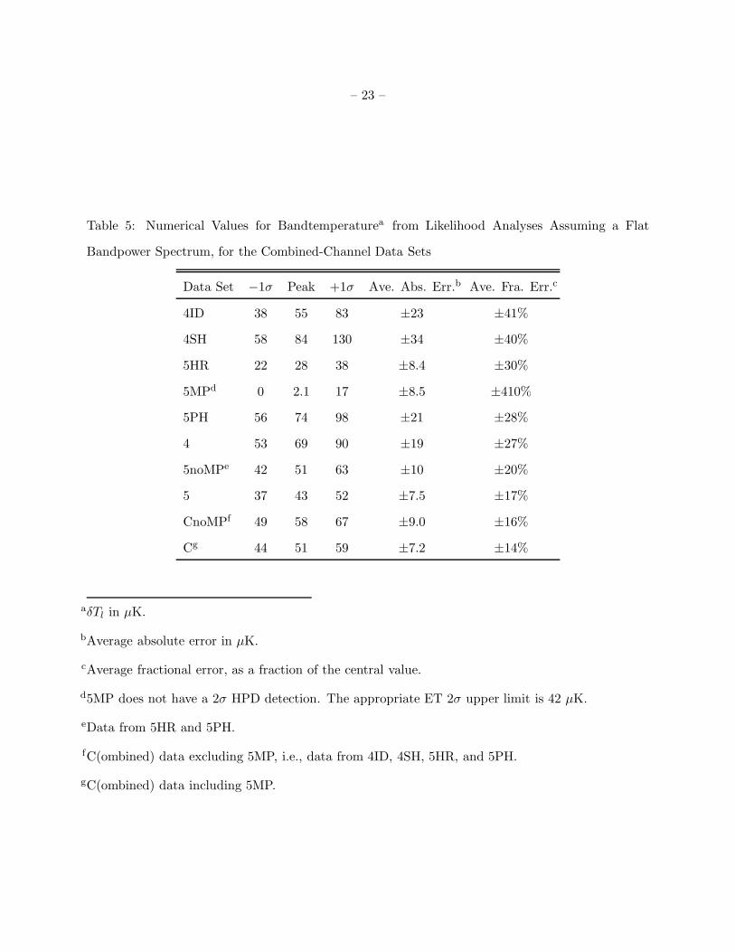
±1σ error bars in µK and as a percentage of the central value. In Table 5 we give the corresponding

numerical values derived from flat bandpower likelihood analyses of the combined-channel MAX

data sets.

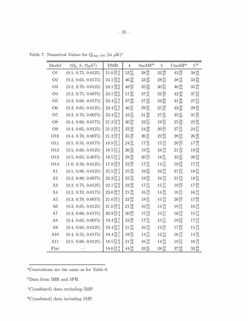
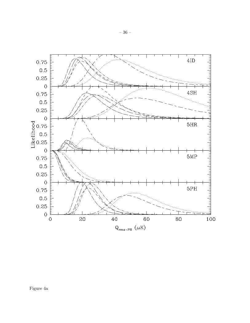
Central values and limits for Qrms−PS are given in Tables 6 and 7 for the various individual

and combined MAX data sets. Some of the likelihood functions used to derive these numerical

values are shown in Figure 4. Tables 6 and 7 also show the results from analyses of the DMR

data, accounting for both statistical and systematic DMR uncertainties (Gorski et al. 1996,1998;

Stompor 1997). The DMR limits quoted are ±2σ HPD for the two extreme data sets: (1)

galactic-frame maps accounting for the high-latitude Galactic emission correction and including

the l = 2 moment in the analysis; and (2) ecliptic-frame maps ignoring the high-latitude Galactic

7 ET limits are determined by integrating the probability density distribution function starting

from 0 µK. The 2σ ET limit encompasses 97.7% of the area. HPD limits are determined by

integrating the probability density distribution function starting at the peak and minimizing the

difference between the upper and lower limits. The 1σ and 2σ HPD limits encompass 68.3% and

95.5% of the area, respectively. See GRGS for a discussion.

– 8 –

correction and excluding the l = 2 moment. The DMR central values quoted are the arithmetic

mean of the ±2σ limits. See Gorski et al. (1998) for a discussion of the DMR central values and

limits.

Tables 8 and 9 give the values of the probability density distribution functions at the peak,

and the marginalized (over Qrms−PS) probability density distribution values for the various

combined-channel MAX data sets.8 The models shown in the figures were chosen on the basis of

their marginal probability distribution values for the C(ombined) MAX data set. Model O1 (an

Ω0 = 0.1, open model) is the most likely model, followed, among the selected models, by Flat (flat

bandpower), O14 (fiducial CDM), models Λ2 and O11 (a spatially-flat, Ω0 = 0.2 model and an

open, Ω0 = 0.5 model), and the least likely one, Λ10 (a flat-Λ, Ω0 = 0.4 model). These selected

models include the most and least likely open and flat-Λ ones among those considered.

3. Results and Discussion

From Table 3 we see that, for those channels with 2σ HPD detections, the rms estimated

from likelihood analyses using flat bandpower spectra is in good agreement with the “sky” rms

estimated from the data, especially for MAX 5. The exception is 4ID 6 cm−1; based on the

SP94 analyses (GRGS), it is unlikely that this can significantly affect conclusions drawn from the

combined MAX data sets.

Tables 4 and 5 give the central values and ±1σ limits on bandtemperature derived from

likelihood analyses with the flat bandpower spectrum. These numerical values can not be

compared directly to those of T96 and L96 because of the many differences in the analyses. For

instance, beamwidth and calibration uncertainties are accounted for in different ways, and T96

use a likelihood ratio method while we use a maximum likelihood method (see T96 for discussion).

Nevertheless, it is reassuring that the largest differences are not greater than ∼ 1σ.

8 These values are computed using a uniform prior in Qrms−PS. The following conclusions are

therefore based solely on the MAX data.

– 9 –

From Tables 4 and 5, we note that the deduced 4SH average absolute uncertainty is larger

than that of the 4SH 9 cm−1 channel and only slightly smaller than the 4SH 3.5 cm−1 one.

Similarly, the deduced 5PH average absolute uncertainty is only slightly smaller than the 5PH 3.5

and 6 cm−1 ones. On the other hand, the average absolute uncertainties do shrink when the 4ID

or 5HR individual-channel data sets are combined.

These error bars only account for instrumental and atmospheric noise, sample variance due

to the limited number of independent data pixels, and beamwidth and calibration uncertainty.

For purely CMB anisotropy data, instrumental and atmospheric noise should integrate down

with more channels of data, sample variance should not, and the beamwidth and calibration

uncertainties are negligible for the purposes of this discussion. Since the MAX 4 3.5 and 6/9 cm−1

window functions are rather dissimilar, an analysis of the behaviour of the error bars in this case

will require a numerical simulation. We focus here on the 5HR and 5PH data sets.

We follow the analysis of §3 of GRGS. In their notation, the total average absolute δTl error

bars for the combined-channel (σtot.,com.) and individual-channel (σtot.,ind.) data sets are, from

Tables 4 and 5,

σ5HRtot.,ind. = 13 µK, σ5HR

tot.,com. = 8.4 µK,

σ5PHtot.,ind. = 22 µK, σ5PH

tot.,com. = 21 µK. (1)

To get this behaviour, the sample variance (σSV) and intrinsic noise (σN) contributions to the δTl

error bars need to be

σ5HRSV = 5.0 µK, σ5HR

N = 12 µK,

σ5PHSV = 20 µK, σ5PH

N = 9.3 µK; (2)

i.e., the 5HR data needs to be dominated by intrinsic noise while the 5PH data needs to be

dominated by sample variance. To see if this is reasonable, we now estimate the MAX 5 sample

variance, following the discussion of GRGS based on the simulations of Netterfield et al. (1995).

We approximate the MAX 5 individual-channel beamwidths by σFWHM = 0.5; the 8 scans then

have 16 independent pixels (with 29 bins, MAX 5 is quite oversampled). With the Netterfield et

– 10 –

al. (1995) 10% simulation correction to the analytic estimate of sample variance (GRGS), the

MAX 5 sample variance is 19% of the δTl central value. Using this, the 5HR and 5PH δTl central

values of Table 5, and the standard equations, we find for the sample variance and intrinsic noise

contributions to the 5HR and 5PH δTl average error bars,

σ5HRSV = 5.3 µK, σ5HR

N = 12 µK,

σ5PHSV = 14 µK, σ5PH

N = 17 µK. (3)

This approximate estimate of the 5HR sample variance and intrinsic noise is very close to what is

needed (eq. [2]) to explain the behaviour of the 5HR error bars. However, eq. (3) indicates that

the 5PH sample variance is not as large as needed (eq. [2]) to explain the behaviour of the 5PH

error bars. While it is premature to read much from such an approximate analysis (GRGS), we

note that the 5PH data were taken at lower balloon altitude and that the 5PH 9 cm−1 data can

not be used for analyses of CMB anisotropy (T96).

We do not record here δTl numerical values for other models from the individual-channel

MAX data sets (the flat bandpower model values are in Table 4). As was the case for SP94

(GRGS), for a given MAX data set the deduced δTl values vary by ∼ 0-10% from model to model,

with a typical range of ∼ 5%. This is significantly smaller than the variations for SuZIE (Ganga

et al. 1997b).

The 5MP data do not show a 2σ HPD detection. Because of the significant non-CMB

component in this data set (L96), and the need for “subtraction” prior to CMB anisotropy analysis

(L96), there is the worry that this data set might be biased. Fortunately, as is seen from the 5,

5noMP, C(ombined), and CnoMP entries in Table 5, inclusion/exclusion of 5MP shifts the deduced

normalization only by ∼ 0.8σ, so 5MP does not significantly affect the final results. We note that

the 5MP upper limit is quite consistent with the 4ID and 5HR detections, but is somewhat below

the 4SH and 5PH detections. Given the discussion about sample variance and intrinsic noise

uncertainties above, we believe that it is more reasonable to include the 5MP results.

Tables 6 – 9 summarize our MAX data set analyses.

– 11 –

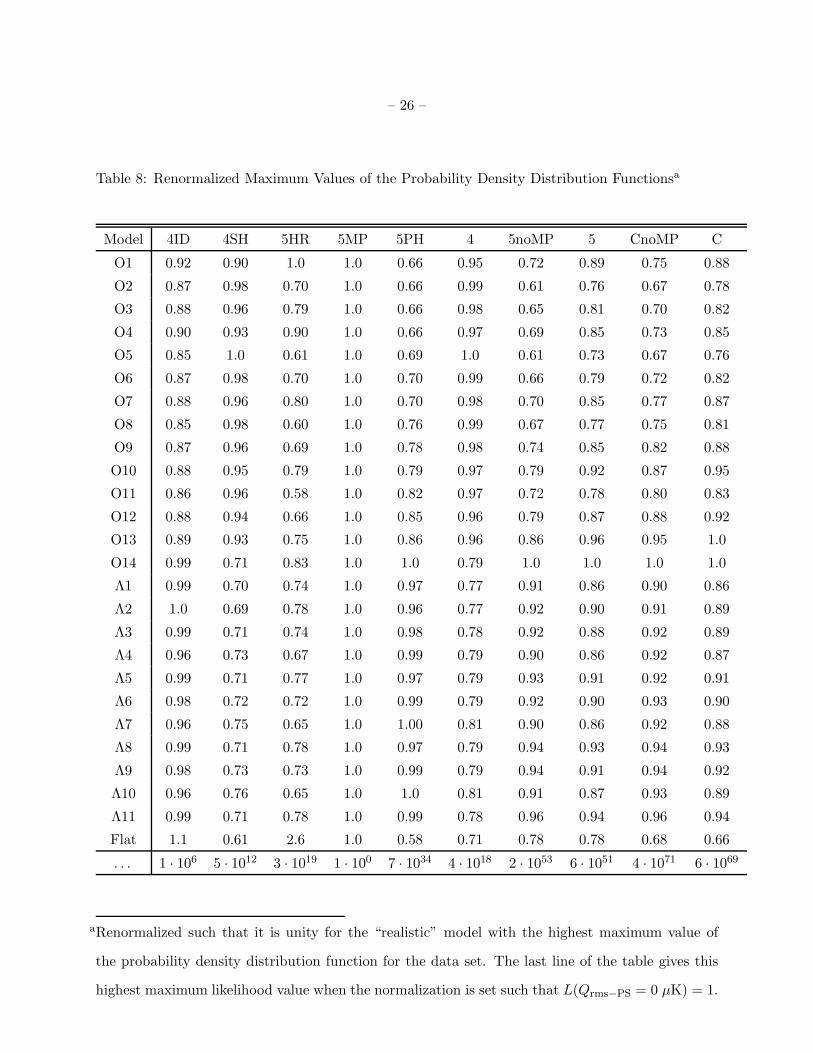
Table 8 lists the maximum values of the probability density distribution function for the

various combined-channel MAX data sets and all models considered here. From these numerical

values, and from Figure 4, one sees that for all the combined-channel MAX data sets, except

5MP which does not have a detection, the likelihood functions are peaked and very well separated

from 0 µK. Note the 14% error bar for the C(ombined) data set in Table 5; the combined MAX

data shows a very significant detection, even after calibration and beamwidth uncertainties are

accounted for. For comparison, depending on model, the corresponding DMR error bars are

∼ 10 − 12% (Gorski et al. 1998). Given such likelihood functions, it is reasonable to choose

between models on the basis of the value of the marginal probability distribution function.

Table 9 lists the marginal probability distribution values for the combined-channel MAX data

sets. In all cases, among all the models considered here, the MAX data favour low-density open

models with Ω0 ∼ 0.1− 0.2 (models O1 – O4).9 This is consistent with what we find from all the

individual-channel MAX data sets (not shown here), and with what is found from an analysis of

the SP94 data (GRGS). Our marginal probability distribution function is evaluated at isolated

points in model-parameter (Ω0, h, ΩBh2) space; assuming it is a gaussian, a model 1σ away from

the most favoured low-density open model CMB anisotropy shape has a marginal value of 0.61,

and a model with marginal value 0.38 is 1.4σ away from the most favoured low-density open

model. The C(ombined) MAX data set values of Table 9 do distinguish between models, although

not at a very significant level.

We conclude that the MAX data are most consistent with the CMB anisotropy shape in

9 Figure 4a shows that the likelihood functions for all the combined-channel MAX data sets are

significantly nongaussian. Consequently, conclusions about model viability based on the marginal

probability density need not be identical to those drawn from the projected probability density.

From Tables 8 and 9 one sees that the projected probability density does not distinguish as much

between models as does the marginal probability distribution, and in fact weakly favours Ω0 = 1

over the open Ω0 = 0.1 case for the C(ombined) data.

– 12 –

low-density open CDM models with Ω0 ∼ 0.1 – 0.3 and 0.4 – 0.5 (with larger h and smaller ΩB),

and with the flat bandpower shape, among the models we consider here. The fiducial CDM and

flat-Λ models have CMB anisotropy spectral shapes which MAX does not favour. This is especially

true for old (t0>∼

15 – 16 Gyr), large baryon density (ΩB>∼0.0175h−2), low-density (Ω0 ∼ 0.2 –

0.4), flat-Λ models. These results are consistent with those based on an analysis of the SP94 data

(GRGS), as well as with earlier analyses of multiple CMB anisotropy data points (Ratra et al.

1997; Ganga et al. 1996; also see Hancock et al. 1997). We emphasize that, under the gaussian

marginal assumption, the MAX data alone do not rule out any of the models we consider here at

the 2σ level.

Tables 6 and 7 list the Qrms−PS values derived from the various combined-channel MAX data

sets. These normalizations are in striking agreement with those deduced from the SP94 data

(GRGS), except for the flat bandpower model where MAX favours a higher normalization than

does SP94. This is further confirmation that the observed CMB anisotropy spectrum rises towards

large l (Scott, Silk, & White 1995; Ratra et al. 1997; Ganga et al. 1996; Netterfield et al. 1997;

Hancock et al. 1997; Page 1997; Lineweaver et al. 1997; Rocha & Hancock 1997).10

For open models with Ω0 ∼ 0.1 − 0.2 the combined MAX data normalization is above the

upper 2σ DMR normalization (Gorski et al. 1998); for Ω0 ∼ 0.1 it is also above the SuZIE

2σ upper limit (Ganga et al. 1997b). For the older (smaller h), higher ΩB, flat-Λ models, the

combined MAX normalization is below the lower 2σ DMR normalization (Stompor 1997). Both of

these results are consistent with earlier CMB anisotropy conclusions (Ratra et al. 1997; Ganga et

al. 1996). An open model with Ω0 ∼ 0.4− 0.5 and h ∼ 0.65 has a CMB anisotropy spectral shape

10 The steepness of the rise towards large l depends on which data sets are included in the

analysis. Hancock et al. (1997), Lineweaver et al. (1997), and Rocha & Hancock (1997) favour

a slightly steeper Cl than do Ganga et al. (1996). This is because Ganga et al. (1996) include a

number of data points (e.g., the four MSAM points and the MAX 3MP point which is consistent

with the repeat 5MP result and the 4ID and 5HR measurements) which favour shallower Cl spectra.

– 13 –

which is not far from what is favoured by the MAX data; in addition, the MAX normalization for

such a model is consistent with what is deduced from the DMR (Gorski et al. 1998) and SP94

data (GRGS), and is also consistent with the SuZIE 2σ upper limit (Ganga et al. 1997b). The

MAX and DMR normalizations also overlap for Ω0 = 1 and some higher h, lower ΩB, low-density

flat-Λ models.

4. Conclusion

We have accounted for beamwidth- and calibration-uncertainty in likelihood analyses of the

MAX 4 and MAX 5 observational data that make use of theoretical CMB spatial anisotropy

spectra in open and spatially-flat Λ CDM cosmogonies. In our analyses, we have assumed that the

appropriately reduced MAX data is purely CMB spatial anisotropy. Other general caveats may be

found in §4 of GRGS, and it is prudent to bear these in mind when interpreting our results.

The marginal probability distribution function values indicate that the MAX data favour

low-density open models over older, high ΩB, low-density, flat-Λ models. However, no model

considered here is ruled out at the 2σ level by the MAX data alone, at least in the gaussian

marginal probability distribution approximation. Combined with results from the analyses of the

DMR, SP94, and SuZIE data, we find that Ω0 ∼ 0.1 − 0.2 open models have CMB anisotropy

spectra shallower than what is favoured by the observations while low h, high ΩB flat-Λ models

have spectra steeper than what is favoured by the observations, in agreement with earlier analyses.

It is interesting that the MAX and SP94 data sets lead to almost identical conclusions for

observationally-motivated low-density open and flat-Λ CDM models. If confirmed, this result

might be of some passing significance.

We acknowledge helpful discussions with A. Clapp, J. Cohn, J. Gundersen, S. Hanany, A.

Lee, G. Rocha, and R. Stompor, as well as, especially, M. Devlin and L. Page. BR acknowledges

support from NSF grant EPS-9550487 with matching support from the state of Kansas and from a

– 14 –

K∗STAR First award. This work was partially carried out at the Infrared Processing and Analysis

Center and the Jet Propulsion Laboratory of the California Institute of Technology, under a

contract with the National Aeronautics and Space Administration.

– 15 –

REFERENCES

Alsop, D. C., et al. 1992, ApJ, 395, 317

Bennett, C. L., et al. 1996, ApJ, 464, L1

Bond, J. R. 1996, in Cosmology and Large Scale Structure, ed. R. Schaeffer, J. Silk, M. Spiro, &

J. Zinn-Justin (Amsterdam: Elsevier Science), 469

Bond, J. R., & Jaffe, A. 1997, in Microwave Background Anisotropies, ed. F. R. Bouchet & T. T.

Van (Gif sur Yvette: Editions Frontieres), in press

Bucher, M., & Cohn, J. D. 1997, Phys. Rev. D, 55, 7461

Bucher, M., Goldhaber, A. S., & Turok, N. 1995, Phys. Rev. D, 52, 3314

Bunn, E. F., & White, M. 1997, ApJ, 480, 6

Cheng, E. S., et al. 1997, ApJ, submitted

Church, S. E., et al. 1997, ApJ, 484, 523

Clapp, A. C., et al. 1994, ApJ, 433, L57

Cole, S., Weinberg, D. H., Frenk, C. S., & Ratra, B. 1997, MNRAS, 289, 37

Devlin, M. J., et al. 1994, ApJ, 430, L1

Dodelson, S., & Stebbins, A. 1994, ApJ, 433, 440

Fischer, M. L., et al. 1992, ApJ, 388, 242

Ganga, K., Page, L., Cheng, E., & Meyer, S. 1994, ApJ, 432, L15

Ganga, K., Ratra, B., & Sugiyama, N. 1996, ApJ, 461, L61

Ganga, K., Ratra, B., Gundersen, J. O., & Sugiyama, N. 1997a, ApJ, 484, 7 (GRGS)

Ganga, K., et al. 1997b, ApJ, 484, 517

Gorski, K. M., et al. 1996, ApJ, 464, L11

Gorski, K. M., Ratra, B., Stompor, R., Sugiyama, N., & Banday, A. J. 1998, ApJS, 114, in press

– 16 –

Gott III, J. R. 1982, Nature, 295, 304

Gott III, J. R. 1997, in Critical Dialogues in Cosmology, ed. N. Turok (Singapore: World

Scientific), in press

Griffin, G. S., et al. 1997, in preparation

Gundersen, J. O., et al. 1993, ApJ, 413, L1

Gundersen, J. O., et al. 1995, ApJ, 443, L57

Guth, A. 1981, Phys. Rev. D, 23, 347

Guth, A. H., & Weinberg, E. J. 1983, Nucl. Phys. B, 212, 321

Gutierrez, C. M., et al. 1997, ApJ, 480, L83

Hancock, S., Rocha, G., Lasenby, A. N., & Gutierrez, C. M. 1997, MNRAS, in press

Harrison, E. R. 1970, Phys. Rev. D, 1, 2726

Kazanas, D. 1980, ApJ, 241, L59

Kitayama, T., & Suto, Y. 1996, ApJ, 469, 480

Klypin, A., Primack, J., & Holtzman, J. 1996, ApJ, 466, 13

Leitch, E. M., Myers, S. T., Readhead, A. C. S., & Pearson, T. J. 1997, in preparation

Lim, M. A., et al. 1996, ApJ, 469, L69 (L96)

Lineweaver, C. H., Barbosa, D., Blanchard, A., & Bartlett, J. G. 1997, A&A, 322, 365

Maddox, S. J., Efstathiou, G., & Sutherland, W. J. 1996, MNRAS, 283, 1227

Maia, M. R. G., & Lima, J. A. S. 1996, Phys. Rev. D, 54, 6111

Masi, S., et al. 1996, ApJ, 463, L47

Meinhold, P. R., et al. 1993a, ApJ, 406, 12

Meinhold, P. R., et al. 1993b, ApJ, 409, L1

Netterfield, C. B., Jarosik, N., Page, L., Wilkinson, D., & Wollack, E. 1995, ApJ, 445, L69

– 17 –

Netterfield, C. B., Devlin, M. J., Jarosik, N., Page, L., & Wollack, E. J. 1997, ApJ, 474, 47

Ostriker, J. P., & Steinhardt, P. J. 1995, Nature, 377, 600

Page, L. A. 1997, astro-ph/9703054

Peacock, J. A. 1997, MNRAS, 284, 885

Peebles, P. J. E., & Yu, J. T. 1970, ApJ, 162, 815

Piccirillo, L., et al. 1997, ApJ, submitted

Platt, S. R., Kovac, J., Dragovan, M., Peterson, J. B., & Ruhl, J. E. 1997, ApJ, 475, L1

Ratra, B., & Peebles, P. J. E. 1994, ApJ, 432, L5

Ratra, B., & Peebles, P. J. E. 1995, Phys. Rev. D, 52, 1837

Ratra, B., Sugiyama, N., Banday, A. J., & Gorski, K. M. 1997, ApJ, 481, 22

Rocha, G., & Hancock, S. 1997, in Microwave Background Anisotropies, ed. F. R. Bouchet & T.

T. Van (Gif sur Yvette: Editions Frontieres), in press

Sato, K. 1981a, Phys. Lett. B, 99, 66

Sato, K. 1981b, MNRAS, 195, 467

Scott, D., Silk, J., & White, M. 1995, Science, 268, 829

Scott, P. F., et al. 1996, ApJ, 461, L1

Srednicki, M., White, M., Scott, D., & Bunn, E. F. 1993, Phys. Rev. Lett., 71, 3747

Stompor, R. 1997, in Microwave Background Anisotropies, ed. F. R. Bouchet & T. T. Van (Gif

sur Yvette: Editions Frontieres), in press

Stompor, R., Gorski, K. M., & Banday, A. J. 1995, MNRAS, 277, 1225

Sugiyama, N. 1995, ApJS, 100, 281

Tanaka, S. T., et al. 1996, ApJ, 468, L81 (T96)

Tanaka, T., & Sasaki, M. 1997, Prog. Theo. Phys., 97, 243

– 18 –

Tucker, G. S., Gush, H. P., Halpern, M., Shinkoda, I., & Towlson, W. 1997, ApJ, 475, L73

Turner, M. S. 1997, in Critical Dialogues in Cosmology, ed. N. Turok (Singapore: World Scientific),

in press

Yamamoto, K., Sasaki, M., & Tanaka, T. 1995, ApJ, 455, 412

Zel’dovich, Ya. B. 1972, MNRAS, 160, 1P

This manuscript was prepared with the AAS LATEX macros v4.0.

– 19 –

Table 1: Numerical Values for the Zero-Lag Window Function Parameters

Channel le−0.5 le lm le−0.5

√

I(Wl)

MAX 4 3.5 cm−1 80 133 145 224 1.51

MAX 4 6/9 cm−1 70 114 127 196 1.41

MAX 5 3.5 cm−1 83 139 150 232 1.55

MAX 5 6/9 cm−1 80 133 146 224 1.51

– 20 –

Table 2: Numerical Values for Parameters Characterizing the Shape of (δTrms2)l

Wl: MAX 4 3.5 cm−1 MAX 4 6/9 cm−1 MAX 5 3.5 cm−1 MAX 5 6/9 cm−1

# (Ω0, h,ΩBh2) le−.5 lm le−.5 le−.5 lm le−.5 le−.5 lm le−.5 le−.5 lm le−.5

(1) (2) (3) (4) (5) (6) (7) (8) (9) (10) (11) (12) (13) (14)

O1 (0.1, 0.75, 0.0125) 54 130 213 42 110 184 57 135 221 54 130 214

O2 (0.2, 0.65, 0.0175) 66 139 222 54 119 192 69 144 230 66 139 222

O3 (0.2, 0.70, 0.0125) 62 135 219 50 115 189 65 141 228 62 135 220

O4 (0.2, 0.75, 0.0075) 57 131 216 47 111 185 60 136 224 57 131 216

O5 (0.3, 0.60, 0.0175) 70 143 226 58 122 195 73 149 235 70 143 227

O6 (0.3, 0.65, 0.0125) 65 139 224 54 118 193 69 145 233 66 140 224

O7 (0.3, 0.70, 0.0075) 60 135 222 50 114 189 63 140 230 61 135 222

O8 (0.4, 0.60, 0.0175) 71 146 229 59 124 198 75 152 237 71 146 229

O9 (0.4, 0.65, 0.0125) 67 143 227 55 120 195 70 149 235 67 143 227

O10 (0.4, 0.70, 0.0075) 61 139 226 50 115 193 64 145 234 61 139 226

O11 (0.5, 0.55, 0.0175) 75 149 230 62 127 200 78 155 237 75 150 230

O12 (0.5, 0.60, 0.0125) 70 147 229 57 124 198 74 153 236 70 148 229

O13 (0.5, 0.65, 0.0075) 64 145 228 52 120 197 68 151 236 65 145 228

O14 (1.0, 0.50, 0.0125) 81 150 216 66 133 196 85 154 220 81 151 216

Λ1 (0.1, 0.90, 0.0125) 85 149 214 74 133 194 88 152 219 85 149 214

Λ2 (0.2, 0.80, 0.0075) 85 149 213 73 134 194 88 153 218 85 150 213

Λ3 (0.2, 0.75, 0.0125) 85 150 215 74 133 195 88 153 220 86 150 215

Λ4 (0.2, 0.70, 0.0175) 86 151 217 75 134 196 89 155 222 86 151 217

Λ5 (0.3, 0.70, 0.0075) 85 150 215 71 134 195 88 154 219 85 151 215

Λ6 (0.3, 0.65, 0.0125) 85 151 216 73 134 196 88 154 221 85 151 216

Λ7 (0.3, 0.60, 0.0175) 86 151 219 74 134 197 89 156 224 86 151 219

Λ8 (0.4, 0.65, 0.0075) 84 151 215 70 134 195 87 155 220 84 151 215

Λ9 (0.4, 0.60, 0.0125) 85 151 216 72 134 196 88 155 221 85 151 217

Λ10 (0.4, 0.55, 0.0175) 86 152 219 74 134 197 89 156 224 86 152 219

Λ11 (0.5, 0.60, 0.0125) 84 151 215 71 134 195 87 155 220 84 151 215

Flat ... 41 103 183 36 90 160 42 106 189 41 103 183

Wl ... 80a 133b 224a 70a 114b 196a 83a 139b 232a 80a 133b 224a

ale−0.5 for the window.

ble for the window.

– 21 –

Table 3: Numerical Values for Rms Temperature Anisotropiesa

Channel “Sky”b FBPc

4ID 3.5 cm−1 71 86

4ID 6 cm−1 29 95

4ID 9 cm−1 55 78

4SH 3.5 cm−1 89 130

4SH 6 cm−1 16 0

4SH 9 cm−1 69 75

5HR 3.5 cm−1 69 62

5HR 6 cm−1 44 40

5HR 9 cm−1 49 56

5PH 3.5 cm−1 64 78

5PH 6 cm−1 85 110

aδTrms in µK.

bEstimated from the data of Fig. 3, as discussed in §2.

cConverted to rms from the results of the likelihood analysis for the flat bandpower (FBP) angular

spectrum, accounting for beamwidth and calibration uncertainties. Note that the 4ID 9 cm−1 and

4SH 6 cm−1 data sets do not have 2σ HPD detections.

– 22 –

Table 4: Numerical Values for Bandtemperaturea from Likelihood Analyses Assuming a Flat

Bandpower Spectrum, for the Individual-Channel Data Sets

Data Set −1σ Peak +1σ Ave. Abs. Err.b Ave. Fra. Err.c

4ID 3.5 cm−1 37 57 86 ±25 ±43%

4ID 6 cm−1 38 67 110 ±37 ±55%

4ID 9 cm−1 d 25 55 110 ±40 ±73%

4SH 3.5 cm−1 58 86 130 ±35 ±41%

4SH 6 cm−1 d 0 0 63 ±32 ...

4SH 9 cm−1 30 53 91 ±31 ±58%

5HR 3.5 cm−1 27 40 58 ±15 ±38%

5HR 6 cm−1 20 27 37 ±8.7 ±33%

5HR 9 cm−1 25 37 55 ±15 ±41%

5PH 3.5 cm−1 32 50 77 ±23 ±45%

5PH 6 cm−1 56 74 99 ±22 ±30%

4 3.5 cm−1 54 71 93 ±19 ±28%

4 6 cm−1 32 55 84 ±26 ±47%

4 9 cm−1 35 54 80 ±22 ±41%

5noMPe 3.5 cm−1 33 44 58 ±12 ±28%

5noMPe 6 cm−1 41 51 63 ±11 ±21%

aδTl in µK.

bAverage absolute error in µK.

cAverage fractional error, as a fraction of the central value.

d4ID 9 cm−1 and 4SH 6 cm−1 do not have 2σ HPD detections; the appropriate ET 2σ upper limits

are 220 µK and 170 µK respectively.

eData from 5HR and 5PH.

– 23 –

Table 5: Numerical Values for Bandtemperaturea from Likelihood Analyses Assuming a Flat

Bandpower Spectrum, for the Combined-Channel Data Sets

Data Set −1σ Peak +1σ Ave. Abs. Err.b Ave. Fra. Err.c

4ID 38 55 83 ±23 ±41%

4SH 58 84 130 ±34 ±40%

5HR 22 28 38 ±8.4 ±30%

5MPd 0 2.1 17 ±8.5 ±410%

5PH 56 74 98 ±21 ±28%

4 53 69 90 ±19 ±27%

5noMPe 42 51 63 ±10 ±20%

5 37 43 52 ±7.5 ±17%

CnoMPf 49 58 67 ±9.0 ±16%

Cg 44 51 59 ±7.2 ±14%

aδTl in µK.

bAverage absolute error in µK.

cAverage fractional error, as a fraction of the central value.

d5MP does not have a 2σ HPD detection. The appropriate ET 2σ upper limit is 42 µK.

eData from 5HR and 5PH.

fC(ombined) data excluding 5MP, i.e., data from 4ID, 4SH, 5HR, and 5PH.

gC(ombined) data including 5MP.

– 24 –

Table 6: Numerical Values for Qrms−PS (in µK)a

Model (Ω0, h, ΩBh2) DMRb 4ID 4SH 5HR 5MP 5PH

O1 (0.1, 0.75, 0.0125) 21.0 25.017.0 43 64

29 61 8943 23 31

18 0 32···

52 6940

O2 (0.2, 0.65, 0.0175) 24.1 28.619.6 38 56

26 54 7838 21 28

16 0 28···

45 6035

O3 (0.2, 0.70, 0.0125) 24.1 28.619.6 40 59

27 57 8240 22 29

17 0 30···

48 6337

O4 (0.2, 0.75, 0.0075) 24.1 28.619.6 42 63

29 60 8842 23 31

18 0 31···

51 6739

O5 (0.3, 0.60, 0.0175) 23.4 27.819.1 31 46

21 44 6331 17 23

13 0 23···

37 4928

O6 (0.3, 0.65, 0.0125) 23.4 27.819.1 33 49

23 47 6833 18 24

14 0 24···

39 5230

O7 (0.3, 0.70, 0.0075) 23.4 27.819.1 35 52

24 50 7335 19 26

15 0 26···

42 5633

O8 (0.4, 0.60, 0.0175) 21.2 24.917.4 25 37

17 36 5225 14 19

11 0 19···

30 4023

O9 (0.4, 0.65, 0.0125) 21.2 24.917.4 27 40

18 38 5627 15 20

11 0 20···

32 4325

O10 (0.4, 0.70, 0.0075) 21.2 24.917.4 29 43

20 41 6029 16 22

12 0 21···

35 4627

O11 (0.5, 0.55, 0.0175) 18.5 21.715.3 20 29

13 28 4120 11 15

8.5 0 14···

24 3118

O12 (0.5, 0.60, 0.0125) 18.5 21.715.3 21 32

15 30 4421 12 16

9.1 0 16···

26 3420

O13 (0.5, 0.65, 0.0075) 18.5 21.715.3 23 34

16 33 4823 13 17

9.8 0 17···

28 3722

O14 (1.0, 0.50, 0.0125) 17.8 20.814.7 18 27

12 27 4019 10 14

7.9 0 14···

23 3118

Λ1 (0.1, 0.90, 0.0125) 25.5 29.721.2 20 30

14 30 4420 12 16

8.8 0 15···

26 3420

Λ2 (0.2, 0.80, 0.0075) 23.3 27.119.4 20 30

14 30 4421 12 16

8.8 0 15···

26 3420

Λ3 (0.2, 0.75, 0.0125) 23.1 27.019.2 19 28

13 27 4119 11 14

8.1 0 14···

24 3118

Λ4 (0.2, 0.70, 0.0175) 23.0 26.819.1 17 26

12 25 3817 10 13

7.6 0 13···

22 2917

Λ5 (0.3, 0.70, 0.0075) 21.0 24.517.5 19 28

13 28 4219 11 15

8.2 0 14···

24 3218

Λ6 (0.3, 0.65, 0.0125) 21.0 24.517.4 17 26

12 26 3818 10 13

7.6 0 13···

22 2917

Λ7 (0.3, 0.60, 0.0175) 20.9 24.417.4 16 24

11 24 3516 9.3 12

7.1 0 12···

20 2716

Λ8 (0.4, 0.65, 0.0075) 19.4 22.716.1 18 28

13 27 4119 11 14

8.0 0 14···

23 3118

Λ9 (0.4, 0.60, 0.0125) 19.4 22.716.1 17 25

12 25 3717 9.7 13

7.4 0 13···

21 2816

Λ10 (0.4, 0.55, 0.0175) 19.4 22.716.1 15 23

11 23 3416 9.0 12

6.8 0 12···

19 2615

Λ11 (0.5, 0.60, 0.0125) 18.5 21.615.3 17 26

12 25 3817 9.8 13

7.5 0 13···

22 2917

Flat · · · 18.6 21.815.4 36 53

24 54 8137 18 25

14 1.3 27···

47 6336

aFor each model, the first of the three entries in each of the last six columns is where the probability

density distribution function peaks. Ellipses as the lower entry in a vertical pair denotes a non-

detection; the upper entry then is the 2σ (97.7% ET) upper limit. For detections, the vertical pair

of numbers are the ±1σ (68.3% HPD) limits, except for DMR where they are ±2σ (95.5% HPD).

bDMR values are from Gorski et al. (1996,1998) and Stompor (1997).

– 25 –

Table 7: Numerical Values for Qrms−PS (in µK)a

Model (Ω0, h, ΩBh2) DMR 4 5noMPb 5 CnoMPc Cd

O1 (0.1, 0.75, 0.0125) 21.0 25.017.0 52 67

40 38 4631 32 38

27 43 5037 38 44

33

O2 (0.2, 0.65, 0.0175) 24.1 28.619.6 46 59

36 33 4028 28 34

24 38 4432 33 38

29

O3 (0.2, 0.70, 0.0125) 24.1 28.619.6 48 62

37 35 4229 30 35

25 40 4634 35 40

31

O4 (0.2, 0.75, 0.0075) 24.1 28.619.6 51 66

40 37 4531 32 38

27 42 4936 37 43

32

O5 (0.3, 0.60, 0.0175) 23.4 27.819.1 37 48

29 27 3323 23 28

20 31 3626 27 31

24

O6 (0.3, 0.65, 0.0125) 23.4 27.819.1 40 51

31 29 3524 25 29

21 33 3828 29 33

25

O7 (0.3, 0.70, 0.0075) 23.4 27.819.1 42 55

33 31 3826 27 31

23 35 4130 31 36

27

O8 (0.4, 0.60, 0.0175) 21.2 24.917.4 30 39

24 22 2718 19 22

16 25 2922 22 26

19

O9 (0.4, 0.65, 0.0125) 21.2 24.917.4 32 42

25 24 2920 20 24

17 27 3123 24 27

21

O10 (0.4, 0.70, 0.0075) 21.2 24.917.4 35 46

27 26 3121 22 26

19 29 3425 26 30

22

O11 (0.5, 0.55, 0.0175) 18.5 21.715.3 24 31

18 17 2115 15 18

13 20 2317 17 20

15

O12 (0.5, 0.60, 0.0125) 18.5 21.715.3 26 33

20 19 2316 16 19

14 21 2518 19 22

16

O13 (0.5, 0.65, 0.0075) 18.5 21.715.3 28 36

22 20 2517 18 21

15 23 2720 20 24

18

O14 (1.0, 0.50, 0.0125) 17.8 20.814.7 22 29

17 17 2114 14 17

12 19 2216 17 19

14

Λ1 (0.1, 0.90, 0.0125) 25.5 29.721.2 25 32

19 19 2316 16 19

14 21 2418 18 21

16

Λ2 (0.2, 0.80, 0.0075) 23.3 27.119.4 25 32

19 19 2316 16 19

14 21 2418 18 21

16

Λ3 (0.2, 0.75, 0.0125) 23.1 27.019.2 23 30

18 17 2114 15 17

12 19 2217 17 20

15

Λ4 (0.2, 0.70, 0.0175) 23.0 26.819.1 21 28

16 16 1913 14 16

12 18 2115 16 18

14

Λ5 (0.3, 0.70, 0.0075) 21.0 24.517.5 23 30

18 18 2115 15 18

13 20 2317 17 20

15

Λ6 (0.3, 0.65, 0.0125) 21.0 24.517.4 21 28

16 16 2013 14 16

12 18 2115 16 18

14

Λ7 (0.3, 0.60, 0.0175) 20.9 24.417.4 20 26

15 15 1812 13 15

11 16 1914 15 17

13

Λ8 (0.4, 0.65, 0.0075) 19.4 22.716.1 23 30

17 17 2114 15 17

12 19 2216 17 19

15

Λ9 (0.4, 0.60, 0.0125) 19.4 22.716.1 21 27

16 16 1913 13 16

11 17 2015 15 18

13

Λ10 (0.4, 0.55, 0.0175) 19.4 22.716.1 19 25

15 14 1712 12 14

10 16 1914 14 16

12

Λ11 (0.5, 0.60, 0.0125) 18.5 21.615.3 21 28

16 16 1913 14 16

12 18 2115 16 18

14

Flat · · · 18.6 21.815.4 44 58

34 33 4127 28 33

24 37 4332 33 38

28

aConventions are the same as for Table 6.

bData from 5HR and 5PH.

cC(ombined) data excluding 5MP.

dC(ombined) data including 5MP.

– 26 –

Table 8: Renormalized Maximum Values of the Probability Density Distribution Functionsa

Model 4ID 4SH 5HR 5MP 5PH 4 5noMP 5 CnoMP C

O1 0.92 0.90 1.0 1.0 0.66 0.95 0.72 0.89 0.75 0.88

O2 0.87 0.98 0.70 1.0 0.66 0.99 0.61 0.76 0.67 0.78

O3 0.88 0.96 0.79 1.0 0.66 0.98 0.65 0.81 0.70 0.82

O4 0.90 0.93 0.90 1.0 0.66 0.97 0.69 0.85 0.73 0.85

O5 0.85 1.0 0.61 1.0 0.69 1.0 0.61 0.73 0.67 0.76

O6 0.87 0.98 0.70 1.0 0.70 0.99 0.66 0.79 0.72 0.82

O7 0.88 0.96 0.80 1.0 0.70 0.98 0.70 0.85 0.77 0.87

O8 0.85 0.98 0.60 1.0 0.76 0.99 0.67 0.77 0.75 0.81

O9 0.87 0.96 0.69 1.0 0.78 0.98 0.74 0.85 0.82 0.88

O10 0.88 0.95 0.79 1.0 0.79 0.97 0.79 0.92 0.87 0.95

O11 0.86 0.96 0.58 1.0 0.82 0.97 0.72 0.78 0.80 0.83

O12 0.88 0.94 0.66 1.0 0.85 0.96 0.79 0.87 0.88 0.92

O13 0.89 0.93 0.75 1.0 0.86 0.96 0.86 0.96 0.95 1.0

O14 0.99 0.71 0.83 1.0 1.0 0.79 1.0 1.0 1.0 1.0

Λ1 0.99 0.70 0.74 1.0 0.97 0.77 0.91 0.86 0.90 0.86

Λ2 1.0 0.69 0.78 1.0 0.96 0.77 0.92 0.90 0.91 0.89

Λ3 0.99 0.71 0.74 1.0 0.98 0.78 0.92 0.88 0.92 0.89

Λ4 0.96 0.73 0.67 1.0 0.99 0.79 0.90 0.86 0.92 0.87

Λ5 0.99 0.71 0.77 1.0 0.97 0.79 0.93 0.91 0.92 0.91

Λ6 0.98 0.72 0.72 1.0 0.99 0.79 0.92 0.90 0.93 0.90

Λ7 0.96 0.75 0.65 1.0 1.00 0.81 0.90 0.86 0.92 0.88

Λ8 0.99 0.71 0.78 1.0 0.97 0.79 0.94 0.93 0.94 0.93

Λ9 0.98 0.73 0.73 1.0 0.99 0.79 0.94 0.91 0.94 0.92

Λ10 0.96 0.76 0.65 1.0 1.0 0.81 0.91 0.87 0.93 0.89

Λ11 0.99 0.71 0.78 1.0 0.99 0.78 0.96 0.94 0.96 0.94

Flat 1.1 0.61 2.6 1.0 0.58 0.71 0.78 0.78 0.68 0.66

. . . 1 · 106 5 · 1012 3 · 1019 1 · 100 7 · 1034 4 · 1018 2 · 1053 6 · 1051 4 · 1071 6 · 1069

aRenormalized such that it is unity for the “realistic” model with the highest maximum value of

the probability density distribution function for the data set. The last line of the table gives this

highest maximum likelihood value when the normalization is set such that L(Qrms−PS = 0 µK) = 1.

– 27 –

Table 9: Renormalized Marginal Values of the Probability Density Distribution Functionsa

Model 4ID 4SH 5HR 5MP 5PH 4 5noMP 5 CnoMP C

O1 1.0 0.99 1.0 1.0 1.0 1.0 1.0 1.0 1.0 1.0

O2 0.83 0.93 0.63 0.88 0.86 0.91 0.74 0.75 0.77 0.78

O3 0.89 0.96 0.74 0.93 0.92 0.95 0.84 0.84 0.86 0.86

O4 0.96 1.0 0.89 0.98 0.97 0.99 0.94 0.94 0.95 0.95

O5 0.67 0.77 0.45 0.71 0.73 0.75 0.60 0.58 0.64 0.62

O6 0.72 0.81 0.55 0.76 0.80 0.79 0.70 0.67 0.73 0.71

O7 0.79 0.86 0.67 0.82 0.86 0.84 0.80 0.78 0.83 0.81

O8 0.55 0.62 0.37 0.58 0.65 0.60 0.55 0.50 0.58 0.53

O9 0.60 0.66 0.45 0.62 0.73 0.64 0.64 0.59 0.68 0.63

O10 0.65 0.71 0.54 0.67 0.80 0.69 0.75 0.70 0.79 0.73

O11 0.43 0.49 0.28 0.45 0.56 0.47 0.46 0.40 0.49 0.43

O12 0.48 0.52 0.34 0.49 0.63 0.50 0.56 0.49 0.58 0.52

O13 0.52 0.56 0.42 0.53 0.70 0.54 0.65 0.58 0.68 0.61

O14 0.47 0.36 0.38 0.42 0.67 0.37 0.63 0.50 0.59 0.50

Λ1 0.51 0.39 0.38 0.46 0.73 0.39 0.64 0.48 0.59 0.48

Λ2 0.52 0.39 0.40 0.47 0.72 0.40 0.64 0.49 0.59 0.49

Λ3 0.47 0.37 0.35 0.43 0.68 0.37 0.59 0.45 0.55 0.45

Λ4 0.43 0.35 0.29 0.40 0.63 0.35 0.54 0.40 0.51 0.41

Λ5 0.48 0.38 0.36 0.44 0.68 0.38 0.61 0.47 0.57 0.47

Λ6 0.44 0.35 0.31 0.40 0.64 0.35 0.56 0.43 0.53 0.43

Λ7 0.40 0.33 0.26 0.37 0.59 0.33 0.50 0.37 0.48 0.38

Λ8 0.47 0.37 0.36 0.43 0.66 0.37 0.60 0.47 0.56 0.47

Λ9 0.43 0.34 0.31 0.39 0.62 0.34 0.54 0.42 0.52 0.42

Λ10 0.38 0.32 0.26 0.36 0.57 0.32 0.49 0.37 0.47 0.38

Λ11 0.44 0.34 0.33 0.40 0.63 0.34 0.57 0.44 0.53 0.44

Flat 1.0 0.62 2.1 0.84 0.82 0.66 0.98 0.78 0.81 0.66

. . . 5 · 107 3 · 1014 5 · 1020 2 · 101 2 · 1036 1 · 1020 2 · 1054 7 · 1052 5 · 1072 7 · 1070

aRenormalized such that it is unity for the “realistic” model with the highest marginal probability

density distribution function value for the data set. The last line of the table gives the marginal

value for the model with highest marginal probability density distribution function value when the

likelihoods are normalized such that L(Qrms−PS = 0 µK) = 1.

– 28 –

FIGURE CAPTIONS

Fig. 1.— CMB anisotropy multipole moments l(l + 1)Cl/(2π) × 1010 (broken lines, scale on left

axis) as a function of multipole l, to l = 600, for selected models O1, O11, O14, Λ2, Λ10, and Flat,

normalized to the DMR maps (Gorski et al. 1996,1998; Stompor 1997). See Table 6 for model-

parameter values. Also shown are the four MAX individual-channel, zero-lag, nominal beamwidth

window functions Wl (solid lines, scale on right axis): MAX 4 6/9 cm−1; MAX 4 3.5 cm−1; MAX 5

6/9 cm−1; and MAX 5 3.5 cm−1 with the Wl peak moving from left to right (the MAX 4 3.5 cm−1

and MAX 5 6/9 cm−1 window functions overlap).

Fig. 2.— (δTrms2)l [= T0

2(2l+1)ClWl/(4π), where T0 is the CMB temperature now] as a function

of l, to l = 400, for (upper panel) the MAX 4 6/9 cm−1 Wl, and for (lower panel) the MAX 5

3.5 cm−1 Wl, for the selected models shown in Fig. 1, normalized to the DMR data. See Tables

2, 6, and 7 for numerical values. Note that the peak sensitivity of an individual-channel window

function corresponds to a different angular scale in each of the models.

Fig. 3.— Individual-channel MAX data (thermodynamic temperature).

Fig. 4.— Likelihood functions, as a function of Qrms−PS for the 6 selected models (O1, O11, O14,

Λ2, Λ10, and Flat) of Fig. 1 (line styles are identical to those used in Figs. 1 and 2), for the

combined-channel MAX data sets. See Table 2 for model-parameter values, and Tables 6 – 9 for

numerical values derived from the corresponding probability density distribution functions.

– 29 –

Figure 1

– 30 –

Figure 2

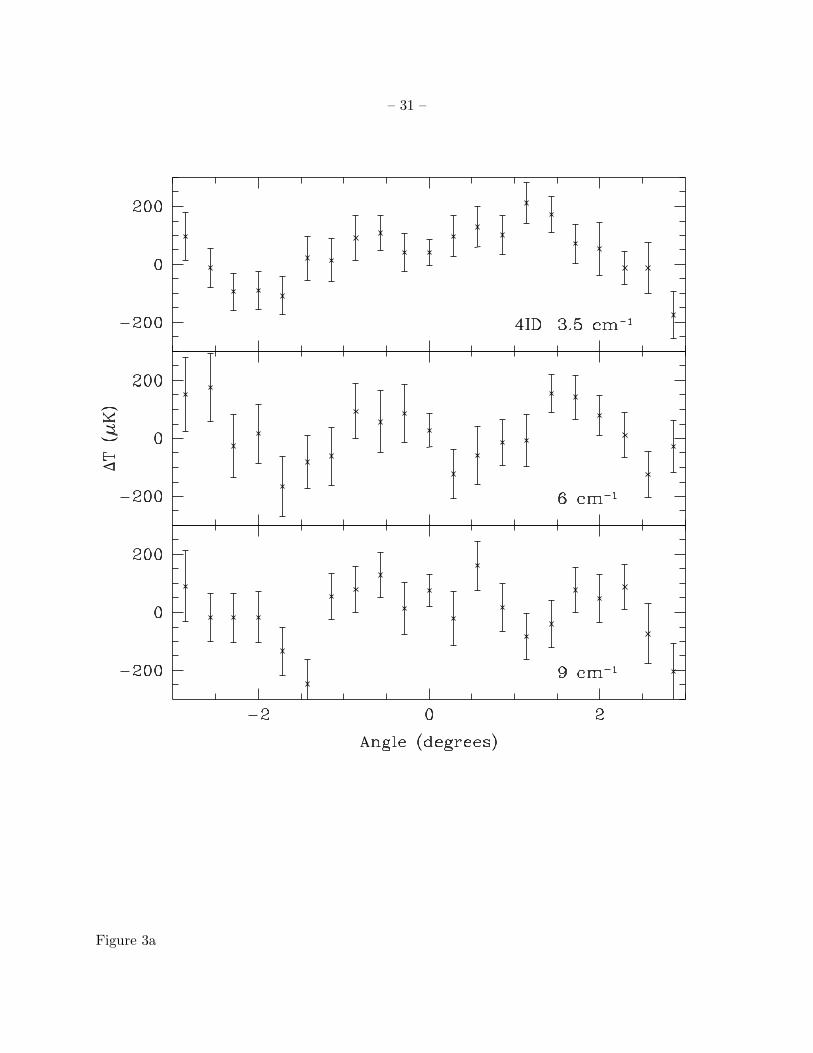
– 31 –

Figure 3a

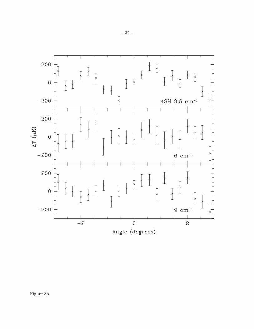
– 32 –

Figure 3b

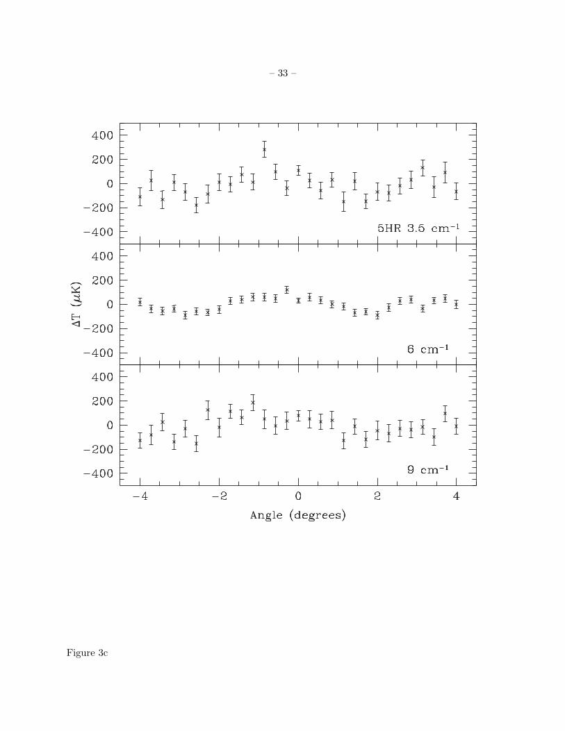
– 33 –

Figure 3c

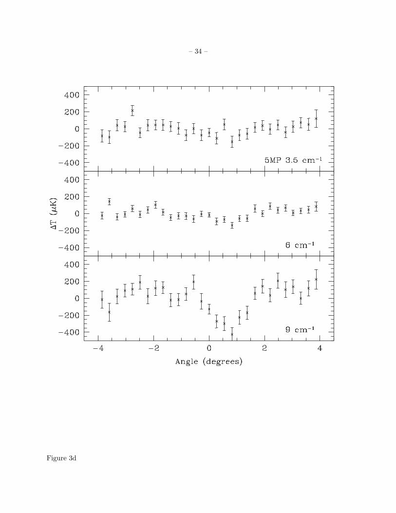
– 34 –

Figure 3d

– 35 –

Figure 3e

– 36 –

Figure 4a

– 37 –

Figure 4b