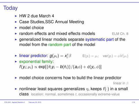
TodayI HW 2 due March 4I Case Studies,SSC Annual MeetingI model choiceI random effects and mixed effects models ELM Ch. 8

I generalized linear models separate systematic part of themodel from the random part of the model

I linear predictor: g(µi) = xTi β E(yi ) = µi ; var(yi ) = φV (µi )

I exponential family:f (yi ;µi) ∝ exp[θiyi − b(θi)/(aiφ) + c(yi , φ)]

I model choice concerns how to build the linear predictorlinear in β

I nonlinear least squares generalizes η, keeps f (·) in a smallclass location: normal, sometimes t , occasionally extreme-value

STA 2201: Applied Statistics II February 25, 2015 1/19

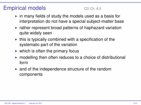
Empirical models CD Ch. 6.5

I in many fields of study the models used as a basis forinterpretation do not have a special subject-matter base

I rather represent broad patterns of haphazard variationquite widely seen

I this is typically combined with a specification of thesystematic part of the variation

I which is often the primary focusI modelling then often reduces to a choice of distributional

formI and of the independence structure of the random

components

STA 2201: Applied Statistics II February 25, 2015 2/19

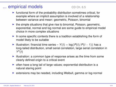
... empirical models CD Ch. 6.5

I functional form of the probability distribution sometimes critical, forexample where an implicit assumption is involved of a relationshipbetween variance and mean: geometric, Poisson, binomial

I the simple situations that give rise to binomial, Poisson, geometric,exponential, normal and log normal are some guide to empirical modelchoice in more complex situations

I In some specific contexts there is a tradition establishing the form ofmodel likely to be suitable

I illustration: financial time series – Y (t) = logP(t)/P(t − 1) has along-tailed distribution, small serial correlation, large serial correlation inY 2(t)

I illustration: a common type of response arises as the time from someclearly defined origin to a critical event

I often have a long tail of large values; exponential distribution is anatural staring point

I extensions may be needed, including Weibull, gamma or log-normal

STA 2201: Applied Statistics II February 25, 2015 3/19

... empirical models CD Ch. 6.5

I often helpful to develop random and systematic parts ofthe model separately

I models should obey natural or known constraints, even ifthese lie outside the range of the data

I example P(Y = 1) = α + βxI often use instead log P(Y =1)

P(Y =0) = α′ + β′xI however, β measures the change in probability per unit

change in xI in many common applications, relationship between y and

several variables x1, . . . xp is involvedI unlikely that the system is wholly linearI impractical to study nonlinear systems of unknown formI therefore reasonable to begin with a linear modelI and seek isolated nonlinearities

STA 2201: Applied Statistics II February 25, 2015 4/19

... empirical models CD Ch. 6.5

I often helpful to develop random and systematic parts ofthe model separately

I naive approach: one random variable per study individualI values for different individuals independentI more realistic: possibility of structure in the random

variationI dependence in time or space, or a hierarchical structure

corresponding to levels of aggregationI ignoring these complications may give misleading

assessments of precision, or bias the conclusions

STA 2201: Applied Statistics II February 25, 2015 5/19

... empirical models CD Ch. 6.5

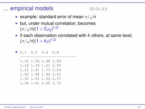
I example: standard error of mean σ/√

nI but, under mutual correlation, becomes

(σ/√

n)(1 + Σρij)1/2

I if each observation correlated with k others, at same level,(σ/√

n)(1 + kρ)1/2

I 0.1 0.2 0.4 0.8--------------------------1.14 1.26 1.48 1.841.18 1.34 1.61 2.051.22 1.41 1.73 2.241.26 1.48 1.84 2.411.30 1.55 1.95 2.571.34 1.61 2.05 2.72

STA 2201: Applied Statistics II February 25, 2015 6/19

... empirical models CD Ch. 6.5

I important to be explicit about the unit of analysisI has a bearing on independence assumptions involved in

model formulationI example: if all patients in the same clinic receive the same

treatmentI then the clinic is the unit of analysisI in some contexts there may be a clear hierarchyI assessment of precision comes primarily from

comparisons between units of analysisI modelling of variation within units is necessary only if of

intrinsic interestI when relatively complex responses are collected on each

study individual, the simplest way of condensing these isthrough a number of summary descriptive measures

I in other situations it may be necessary to representexplicitly the different hierarchies of variation

STA 2201: Applied Statistics II February 25, 2015 7/19

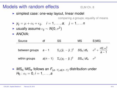
Models with random effects ELM Ch. 8

I simplest case: one-way layout, linear modelcomparing a groups; equality of means

I yij = µ+ αi + εij , i = 1, . . . ,a; j = 1, . . .nI usually assume εij ∼ N(0, σ2)

I ANOVA:

Source df SS MS E(MS)

between groups a− 1 Σij (yi. − y..)2 SSb/dfb σ2 +nΣiα

2i

a− 1

within groups a(n − 1) Σij (yij − yi.)2 SSw/dfw σ2

I MSb/MSw follows an F(a−1),a(n−1) distribution underH0 : αi = 0, i = 1, . . . ,a

STA 2201: Applied Statistics II February 25, 2015 8/19

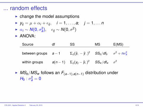
... random effectsI change the model assumptionsI yij = µ+ αi + εij , i = 1, . . . ,a; j = 1, . . .nI αi ∼ N(0, σ2

a), εij ∼ N(0, σ2)

I ANOVA:

Source df SS MS E(MS)

between groups a− 1 Σij (yi. − y..)2 SSb/dfb σ2 + nσ2a

within groups a(n − 1) Σij (yij − yi.)2 SSw/dfw σ2

I MSb/MSw follows an F(a−1),a(n−1) distribution underH0 : σ2

a = 0

STA 2201: Applied Statistics II February 25, 2015 9/19

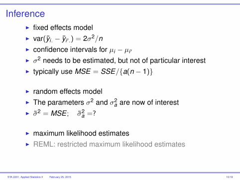
InferenceI fixed effects modelI var(yi. − yi ′.) = 2σ2/nI confidence intervals for µi − µi ′

I σ2 needs to be estimated, but not of particular interestI typically use MSE = SSE/a(n − 1)

I random effects modelI The parameters σ2 and σ2

a are now of interestI σ2 = MSE ; σ2

a =?

I maximum likelihood estimatesI REML: restricted maximum likelihood estimates

STA 2201: Applied Statistics II February 25, 2015 10/19

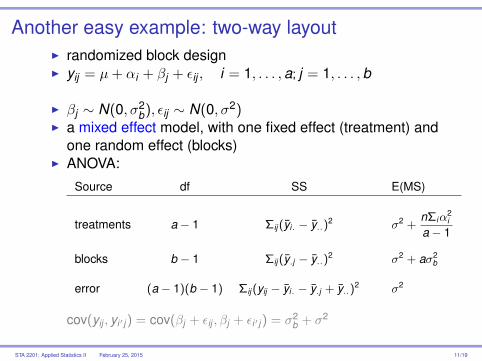
Another easy example: two-way layoutI randomized block designI yij = µ+ αi + βj + εij , i = 1, . . . ,a; j = 1, . . . ,b

I βj ∼ N(0, σ2b), εij ∼ N(0, σ2)

I a mixed effect model, with one fixed effect (treatment) andone random effect (blocks)

I ANOVA:Source df SS E(MS)

treatments a− 1 Σij (yi. − y..)2 σ2 +nΣiα

2i

a− 1

blocks b − 1 Σij (y.j − y..)2 σ2 + aσ2b

error (a− 1)(b − 1) Σij (yij − yi. − y.j + y..)2 σ2

cov(yij , yi′ j ) = cov(βj + εij , βj + εi′ j ) = σ2b + σ2

STA 2201: Applied Statistics II February 25, 2015 11/19

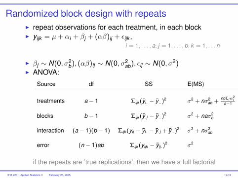
Randomized block design with repeatsI repeat observations for each treatment, in each blockI yijk = µ+ αi + βj + (αβ)ij + εijk ,

i = 1, . . . , a; j = 1, . . . , b; k = 1, . . . n

I βj ∼ N(0, σ2b), (αβ)ij ∼ N(0, σ2

ab), εij ∼ N(0, σ2)I ANOVA:

Source df SS E(MS)

treatments a− 1 Σijk (yi. − y..)2 σ2 + nσ2ab +

nbΣiα2i

a−1

blocks b − 1 Σijk (y.j − y..)2 σ2 + naσ2b

interaction (a− 1)(b − 1) Σijk (yij − yi. − y.j + y..)2 σ2 + nσ2ab

error (n − 1)ab Σijk (yijk − yij.)2 σ2

if the repeats are ’true replications’, then we have a full factorial

STA 2201: Applied Statistics II February 25, 2015 12/19

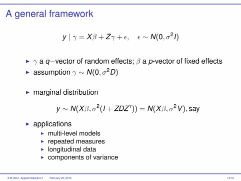
A general framework

y | γ = Xβ + Zγ + ε, ε ∼ N(0, σ2I)

I γ a q−vector of random effects; β a p-vector of fixed effectsI assumption γ ∼ N(0, σ2D)

I marginal distribution

y ∼ N(Xβ, σ2(I + ZDZ T)) = N(Xβ, σ2V ), say

I applicationsI multi-level modelsI repeated measuresI longitudinal dataI components of variance

STA 2201: Applied Statistics II February 25, 2015 13/19

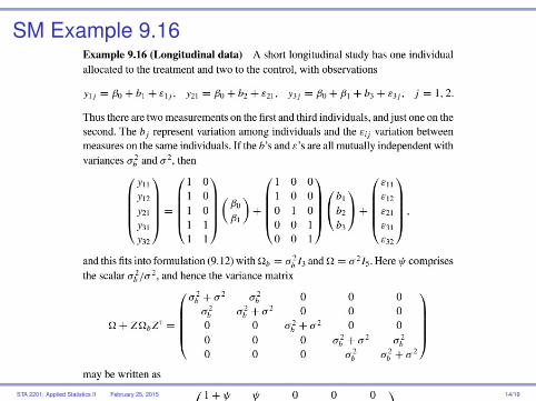
SM Example 9.16

STA 2201: Applied Statistics II February 25, 2015 14/19

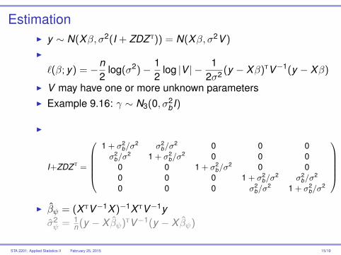
EstimationI y ∼ N(Xβ, σ2(I + ZDZ T)) = N(Xβ, σ2V )

I

`(β; y) = −n2

log(σ2)− 12

log |V | − 12σ2 (y − Xβ)TV−1(y − Xβ)

I V may have one or more unknown parametersI Example 9.16: γ ∼ N3(0, σ2

bI)

I

I+ZDZ T =

1 + σ2

b/σ2 σ2

b/σ2 0 0 0

σ2b/σ

2 1 + σ2b/σ

2 0 0 00 0 1 + σ2

b/σ2 0 0

0 0 0 1 + σ2b/σ

2 σ2b/σ

2

0 0 0 σ2b/σ

2 1 + σ2b/σ

2

I βψ = (X TV−1X )−1X TV−1yσ2ψ = 1

n (y − X βψ)TV−1(y − X βψ)

STA 2201: Applied Statistics II February 25, 2015 15/19

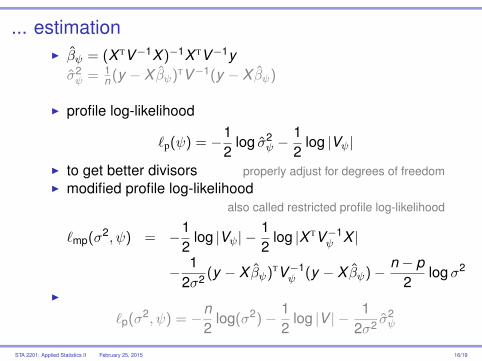
... estimationI βψ = (X TV−1X )−1X TV−1yσ2ψ = 1

n (y − X βψ)TV−1(y − X βψ)

I profile log-likelihood

`p(ψ) = −12

log σ2ψ −

12

log |Vψ|

I to get better divisors properly adjust for degrees of freedomI modified profile log-likelihood

also called restricted profile log-likelihood

`mp(σ2, ψ) = −12

log |Vψ| −12

log |X TV−1ψ X |

− 12σ2 (y − X βψ)TV−1

ψ (y − X βψ)− n − p2

logσ2

I

`p(σ2, ψ) = −n2

log(σ2)− 12

log |V | − 12σ2 σ

2ψ

STA 2201: Applied Statistics II February 25, 2015 16/19

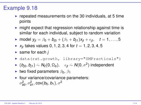
Example 9.18I repeated measurements on the 30 individuals, at 5 time

pointsI might expect that regression relationship against time is

similar for each individual, subject to random variationI model yjt = β0 + bj0 + (β1 + bj1)xjt + εjt , t = 1, . . . ,5I xjt takes values 0,1,2,3,4 for t = 1,2,3,4,5I same for each jI data(rat.growth, library="SMPracticals")

I (bj0,bj1).∼ N2(0,Ωb), εjt

.∼ N(0, σ2) independentI two fixed parameters β0, β1

I four variance/covariance parameters:σ2

b0, σ2b1, cov(b0,b1), σ2

STA 2201: Applied Statistics II February 25, 2015 17/19

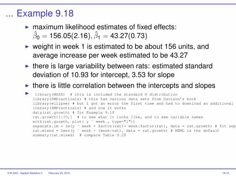
... Example 9.18I maximum likelihood estimates of fixed effects:β0 = 156.05(2.16), β1 = 43.27(0.73)

I weight in week 1 is estimated to be about 156 units, andaverage increase per week estimated to be 43.27

I there is large variability between rats: estimated standarddeviation of 10.93 for intercept, 3.53 for slope

I there is little correlation between the intercepts and slopesI library(MASS) # this is included the standard R distribution

library(SMPracticals) # this has various data sets from Davison’s booklibrary(ellipse) # but I got an error the first time and had to download an additional packagelibrary(SMPracticals) # and now it worksdata(rat.growth) # for Example 9.18rat.growth[1:10,] # to see what it looks like, and to see variable nameswith(rat.growth, plot( y ˜ week , type="l"))separate.lm = lm(y ˜ week + factor(rat)+ week:factor(rat), data = rat.growth) # fit separate linear models to each set of 5 observationsrat.mixed = lmer(y ˜ week + (week|rat), data = rat.growth) # REML is the defaultsummary(rat.mixed) # compare Table 9.28

STA 2201: Applied Statistics II February 25, 2015 18/19