AN INTRODUCTION TO MEASURE THEORY AND PROBABILITY
207
AN INTRODUCTION TO MEASURE THEORY AND PROBABILITY Luigi Ambrosio, Giuseppe Da Prato, Andrea Mennucci
Transcript of AN INTRODUCTION TO MEASURE THEORY AND PROBABILITY
AN INTRODUCTION TO MEASURETHEORY AND PROBABILITY
Luigi Ambrosio, Giuseppe Da Prato, Andrea Mennucci
Contents
1 Measure spaces 11.1 Algebras and σ–algebras of sets . . . . . . . . . . . . . . . . . . . . . 1
1.1.1 Notation and preliminaries . . . . . . . . . . . . . . . . . . . . 11.1.2 Rings, algebras and σ–algebras . . . . . . . . . . . . . . . . . 2
1.2 Additive and σ–additive functions . . . . . . . . . . . . . . . . . . . . 41.2.1 Measurable spaces and measure spaces . . . . . . . . . . . . . 6
1.3 The basic extension theorem . . . . . . . . . . . . . . . . . . . . . . . 81.3.1 π–systems and Dynkin systems . . . . . . . . . . . . . . . . . 81.3.2 The outer measure . . . . . . . . . . . . . . . . . . . . . . . . 10
1.4 The Lebesgue measure in
. . . . . . . . . . . . . . . . . . . . . . . 131.5 Inner and outer regularity of measures on metric spaces . . . . . . . . 16
2 Integration 212.1 Inverse image of a function . . . . . . . . . . . . . . . . . . . . . . . . 212.2 Measurable and Borel functions . . . . . . . . . . . . . . . . . . . . . 222.3 Partitions and simple functions . . . . . . . . . . . . . . . . . . . . . 232.4 Integral of a nonnegative E –measurable function . . . . . . . . . . . . 24
2.4.1 Integral of simple functions . . . . . . . . . . . . . . . . . . . 242.4.2 The repartition function . . . . . . . . . . . . . . . . . . . . . 262.4.3 The archimedean integral . . . . . . . . . . . . . . . . . . . . 282.4.4 Integral of a nonnegative E –measurable function . . . . . . . . 29
2.5 Integral of functions with a variable sign . . . . . . . . . . . . . . . . 322.6 Convergence of integrals . . . . . . . . . . . . . . . . . . . . . . . . . 33
2.6.1 Uniform integrability and Vitali convergence theorem . . . . . 342.7 A characterization of Riemann integrable functions . . . . . . . . . . 36
3 Lp spaces 413.1 Spaces L 1(X, E , µ) and L1(X, E , µ) . . . . . . . . . . . . . . . . . . 413.2 Spaces Lp(X, E , µ) with p ∈ (1,∞] . . . . . . . . . . . . . . . . . . . 44
3.2.1 Holder and Minkowski inequalities . . . . . . . . . . . . . . . 47
i
ii
3.3 Convergence in L1(X, E , µ) . . . . . . . . . . . . . . . . . . . . . . . . 49
3.4 Dense subsets of Lp(X, E , µ) . . . . . . . . . . . . . . . . . . . . . . . 49
4 Hilbert spaces 53
4.1 Scalar products, pre-Hilbert and Hilbert spaces . . . . . . . . . . . . 53
4.2 The projection theorem . . . . . . . . . . . . . . . . . . . . . . . . . . 55
4.3 Linear continuous functionals . . . . . . . . . . . . . . . . . . . . . . 57
4.4 Bessel inequality, Parseval identity and orthonormal systems . . . . . 59
5 Fourier series 63
5.1 Pointwise convergence of the Fourier series . . . . . . . . . . . . . . . 64
5.2 Completeness of the trigonometric system . . . . . . . . . . . . . . . 68
6 Operations on measures 71
6.1 The product measure and Fubini–Tonelli theorem . . . . . . . . . . . 71
6.2 The Lebesgue measure onn . . . . . . . . . . . . . . . . . . . . . . 74
6.3 Countable products . . . . . . . . . . . . . . . . . . . . . . . . . . . . 77
6.4 Comparison of measures . . . . . . . . . . . . . . . . . . . . . . . . . 82
6.5 Signed measures . . . . . . . . . . . . . . . . . . . . . . . . . . . . . . 88
6.6 Measures in
. . . . . . . . . . . . . . . . . . . . . . . . . . . . . . . 92
6.7 Convergence of measures on
. . . . . . . . . . . . . . . . . . . . . . 93
6.8 Fourier transform . . . . . . . . . . . . . . . . . . . . . . . . . . . . . 99
6.8.1 Fourier transform of a measure . . . . . . . . . . . . . . . . . 100
7 The fundamental theorem of the integral calculus 105
8 Measurable transformations 113
8.1 Image measure . . . . . . . . . . . . . . . . . . . . . . . . . . . . . . 113
8.2 Change of variables in multiple integrals . . . . . . . . . . . . . . . . 114
8.3 Image measure of L n by a C1 diffeomorphism . . . . . . . . . . . . . 115
9 General concepts of Probability 121
9.1 Probability spaces and random variables . . . . . . . . . . . . . . . . 121
9.2 Expectation, variance and standard deviation . . . . . . . . . . . . . 124
9.3 Law and characteristic function of a random variable . . . . . . . . . 128
10 Conditional probability and independence 135
10.1 Independence of events, σ–algebras, random variables . . . . . . . . . 136
10.1.1 Indipendence of real valued variables . . . . . . . . . . . . . . 141
10.2 Independent sequences with prescribed laws . . . . . . . . . . . . . . 143
iii
11 Convergence of random variables 14911.1 Convergence in probability . . . . . . . . . . . . . . . . . . . . . . . . 14911.2 Convergence in law . . . . . . . . . . . . . . . . . . . . . . . . . . . . 152
12 Sequences of independent variables 15512.1 Sequences of independent events . . . . . . . . . . . . . . . . . . . . . 15512.2 The law of large numbers . . . . . . . . . . . . . . . . . . . . . . . . . 15812.3 Some applications of Probability theory . . . . . . . . . . . . . . . . . 162
12.3.1 Density of Bernstein polynomials . . . . . . . . . . . . . . . . 16212.3.2 The Monte Carlo method . . . . . . . . . . . . . . . . . . . . 16312.3.3 Empirical distribution . . . . . . . . . . . . . . . . . . . . . . 164
12.4 The central limit theorem . . . . . . . . . . . . . . . . . . . . . . . . 164
13 Stationary sequences and elements of ergodic theory 16913.1 Stationary sequences and law of large numbers . . . . . . . . . . . . . 16913.2 Measure-preserving transformations and ergodic theorems . . . . . . . 173
13.2.1 Ergodic processes . . . . . . . . . . . . . . . . . . . . . . . . . 17613.3 Examples . . . . . . . . . . . . . . . . . . . . . . . . . . . . . . . . . 177
13.3.1 Arithmetic progressions on the circle . . . . . . . . . . . . . . 17713.3.2 Geometric progressions on the circle . . . . . . . . . . . . . . . 17913.3.3 The triangular map . . . . . . . . . . . . . . . . . . . . . . . . 18013.3.4 The logistic map . . . . . . . . . . . . . . . . . . . . . . . . . 181
14 Brownian motion 18514.1 Discrete random walks . . . . . . . . . . . . . . . . . . . . . . . . . . 18514.2 Some properties of Gaussian random variables . . . . . . . . . . . . . 18714.3 d-dimensional Brownian motion . . . . . . . . . . . . . . . . . . . . . 19114.4 Total variation of the Brownian motion . . . . . . . . . . . . . . . . . 198
Chapter 1
Measure spaces
1.1 Algebras and σ–algebras of sets
1.1.1 Notation and preliminaries
We shall denote by X a non-empty set, by P(X) the set of all parts of X and by∅ the empty set. For any subset A of X we shall denote by Ac its complementAc := x ∈ X : x /∈ A . If A, B ∈ P(X) we set A \ B := A ∩ Bc and A∆B :=(A \B) ∪ (B \ A).
Let (An) be a sequence in P(X). Then the following De Morgan identity holds,
(∞⋃
n=0
An
)c
=∞⋂
n=0
Acn.
Moreover, we define (1)
lim supn→∞
An :=
∞⋂
n=0
∞⋃
m=n
Am, lim infn→∞
An :=
∞⋃
n=0
∞⋂
m=n
Am.
As it can be easily checked, lim supn→∞
An (resp. lim infn→∞
An) consists of those elements
of X that belong to infinitely many An (resp. that belong to all but finitely manyAn).
If L := lim supn→∞
An = lim infn→∞
An we set L = limn→∞
An and we say that (An)
converges to L (we shall write in this case An → L).
(1)Notice the analogy with liminf and limsup limits for a sequence (an) of real numbers. We havelim sup
n→∞an = inf
n∈supm≥n
am and lim infn→∞
an = supn∈
infm≥n
am. This is something more than an analogy,
see Exercise 1.1.
1

2 Measure spaces
It easy to check that if (An) is nondecreasing (i.e. An ⊂ An+1, n ∈ ), we have
limn→∞
An =∞⋃
n=0
An,
whereas if (An) is nonincreasing (i.e. An ⊃ An+1, n ∈ ), we have
limn→∞
An =
∞⋂
n=0
An.
In the first case we shall write An ↑ L, and in the second one An ↓ L.
1.1.2 Rings, algebras and σ–algebras
Definition 1.1 (Rings and Algebras) A non empty subset A of P(X) is saidto be a ring if:
(i) ∅ belongs to A ;
(ii) A, B ∈ A =⇒ A ∪ B, A ∩B ∈ A ;
(iii) A, B ∈ A =⇒ A \B ∈ A .
We say that a ring is an algebra if X ∈ A .
Notice that rings are stable only with respect to relative complement, whereasalgebras are stable under complement in X.
Let K ⊂ P(X). As the intersection of any family of algebras is still an algebra,the minimal algebra including K (that is the intersection of all algebras includingK ) is well defined, and called the algebra generated by K . A constructive char-acterization of the algebra generated by K can be easily achieved as follows: setF (0) = K ∪ ∅, X and
F (i+1) :=⋃
A ∪ B,A ∩ B,Ac : A, B ∈ F (i)
∀i ≥ 0.
Then, the algebra A generated by K is given by∞⋃i=0
F (i). Indeed, it is immediate
to check by induction on i that A ⊃ F (i), and therefore the union of the F (i)’s iscontained in A . On the other hand, this union is easily seen to be an algebra, sothe minimality of A provides the opposite inclusion.
Definition 1.2 (σ-algebras) A non-empty subset E of P(X) is said to be a σ–algebra if:
Chapter 1 3
(i) E is an algebra;
(ii) if (An) is a sequence of elements of E then∞⋃
n=0
An ∈ E .
If E is a σ–algebra and (An) ⊂ E we have∞⋂
n=0
An ∈ E by the De Morgan
identity. Moreover, both sets
lim infn→∞
An, lim supn→∞
An,
belong to E .Obviously, ∅, X and P(X) are σ–algebras, respectively the smallest and the
largest ones. Let K be a subset of P(X). As the intersection of any family ofσ-algebras is still a σ-algebra, the minimal σ–algebra including K (that is theintersection of all σ–algebras including K ) is well defined, and called the σ–algebragenerated by K . It is denoted by σ(K ).
In contrast with the case of generated algebras, it is quite hard to give a con-structive characterization of the generated σ-algebras: this requires the transfiniteinduction and it is illustrated in Exercise 1.11.
Definition 1.3 (Borel σ-algebra) If (E, d) is a metric space, the σ–algebra gen-erated by all open (resp. closed) subsets of E is called the Borel σ–algebra of E andit is denoted by B(E).
In the case when E =
the Borel σ-algebra has a particularly simple class ofgenerators.
Example 1.4 (B()) Let I be the set of all semi–closed intervals [a, b) with a ≤ b.
Then σ(I ) coincides with B(). In fact σ(I ) contains all open intervals (a, b) since
(a, b) =
∞⋃
n=n0
[a +
1
n, b),
where 1n0
< b − a. Moreover, any open set A in
is a countable union of open
intervals. (2) An analogous argument proves that B() is generated by semi-closed
intervals (a, b], by open intervals, by closed intervals and even by open or closedhalf-lines.
(2)Indeed, let (ak) be a sequence including all rational numbers of A and denote by Ik the largestopen interval contained in A and containing ak. We clearly have A ⊃ ⋃∞
k=0 Ik, but also the oppositeinclusion holds: it suffices to consider, for any x ∈ A, r > 0 such that (x − r, x + r) ⊂ A, and ksuch that ak ∈ (x− r, x+ r) to obtain (x− r, x+ r) ⊂ Ik, by the maximality of Ik, and then x ∈ Ik.
4 Measure spaces
1.2 Additive and σ–additive functions
Let A ⊂ P(X) be a ring and let µ be a mapping from A into [0,+∞] such thatµ(∅) = 0. We say that µ is additive if for any n ∈
and mutually disjoint setsA1, . . . , An ∈ A , we have
µ
(n⋃
k=1
Ak
)=
n∑
k=1
µ(Ak).
If µ is additive, A, B ∈ F and A ⊃ B, we have µ(A) = µ(B) + µ(A \ B), so thatµ(A) ≥ µ(B). Therefore any additive function is nondecreasing with respect to setinclusion.
An additive function µ on A is called σ–additive if for any sequence (An) ⊂ A
of mutually disjoint sets such that∞⋃
n=0
An ∈ A we have
µ
(∞⋃
n=0
An
)=
∞∑
n=0
µ(An).
Remark 1.5 (σ–additivity and σ–subadditivity) Let µ be additive on a ring
A and let (An) ⊂ A be mutually disjoint and such that∞⋃
n=0
An ∈ A . Then by
monotonicity we have
µ
(∞⋃
n=0
An
)≥
k∑
n=0
µ(An), for all k ∈ .
Therefore
µ
(∞⋃
n=0
An
)≥
∞∑
n=0
µ(An).
Thus, to show that an additive function is σ–additive, it is enough to prove that itis σ–subadditive, that is
µ(B) ≤∞∑
k=0
µ(Ak),
for any B ∈ A and any sequence (An) ⊂ A such that B ⊂∞⋃
n=0
An.
Let µ be additive on A . Then σ–additivity of µ is equivalent to continuity of µin the sense of the following proposition.
Chapter 1 5
Proposition 1.6 (Continuity on nondecreasing sequences) If µ is additive ona ring A , then (i) ⇐⇒ (ii), where:
(i) µ is σ–additive;
(ii) (An) ⊂ A and A ∈ A , An ↑ A =⇒ µ(An) ↑ µ(A).
Proof. (i)=⇒(ii). In the proof of this implication we can assume with no loss ofgenerality that µ(An) <∞ for all n ∈
. Let (An) ⊂ A , A ∈ A , An ↑ A. Then
A = A0 ∪∞⋃
n=0
(An+1 \ An),
the unions being disjoint. Since µ is σ–additive, we deduce that
µ(A) = µ(A0) +∞∑
n=0
(µ(An+1) − µ(An)) = limn→∞
µ(An),
and (ii) follows.
(ii)=⇒(i). Let (An) ⊂ A be mutually disjoint and such that A : =∞⋃
k=0
Ak ∈ A .
Set
Bm =m⋃
k=0
Ak.
Then Bm ↑ A and µ(Bm) =m∑
k=0
µ(Ak) ↑ µ(A) by the assumption. This implies (i).
Proposition 1.7 (Continuity on nonincreasing sequences) Let µ be σ–additiveon a ring A . Then
(An) ⊂ A and A ∈ A , An ↓ A, µ(A0) <∞ =⇒ µ(An) ↓ µ(A). (1.1)
Proof. Setting Bn := A0 \ An, B := A0 \ A, we have Bn ↑ B, therefore theprevious proposition gives µ(Bn) ↑ µ(B). As µ(An) = µ(A0) − µ(Bn) and µ(A) =µ(A0) − µ(B) the proof is achieved.
Corollary 1.8 (Upper and lower semicontinuity of the measure) Let µ be σ–additive on a σ–algebra E and let (An) ⊂ E . Then we have
µ(lim infn→∞
An
)≤ lim inf
n→∞µ(An) (1.2)
6 Measure spaces
and, if µ(X) <∞, we have also
lim supn→∞
µ(An) ≤ µ
(lim sup
n→∞An
). (1.3)
In particular An → A =⇒ µ(An) → µ(A).
Proof. Set L = lim supn→∞
An. Then we can write L =∞⋂
n=1
Bn, where Bn =∞⋃
m=n
Am ↓ L.Now, assuming µ(X) <∞, by Proposition 1.7 it follows that
µ(L) = limn→∞
µ(Bn) = infn∈
µ(Bn) ≥ infn∈
supm≥n
µ(Am) = lim supn→∞
µ(An).
Thus, we have proved (1.3). The inequality (1.2) can be proved similarly usingProposition 1.6, thus without using the assumption µ(X) <∞.
The following result is very useful to estimate the measure of a lim sup of sets.
Lemma 1.9 (Borel–Cantelli) Let µ be σ–additive on a σ–algebra E and let (An)
be a sequence of subsets of E . Assume that∞∑
n=0
µ(An) <∞. Then
µ
(lim sup
n→∞An
)= 0.
Proof. Set L = lim supn→∞
An. Then L =∞⋂
n=1
Bn, where Bn :=∞⋃
m=n
Am ↓ L. Conse-
quently
µ(L) ≤ µ(Bn) ≤∞∑
m=n
µ(Am),
for all n ∈ . As n→ ∞ we find µ(L) = 0.
1.2.1 Measurable spaces and measure spaces
Let E be a σ–algebra of subsets of X. Then we say that the pair (X, E ) is a measur-able space. Let µ : E → [0,+∞] be a σ–additive function. Then we call µ a measureon (X, E ), and we call the triple (X, E , µ) a measure space.
The measure µ is said to be finite if µ(X) <∞, σ–finite if there exists a sequence
(An) ⊂ E such that∞⋃
n=0
An = X and µ(An) < ∞ for all n ∈ . Finally, µ is called
a probability measure if µ(X) = 1.
Chapter 1 7
The simplest (but fundamental) example of a probability measure is the Diracmass δx, defined by
δx(B) :=
1 if x ∈ B
0 if x /∈ B.
This example can be generalized as follows, see also Exercise 1.5.
Example 1.10 (Discrete measures) Assume that Y ⊂ X is a finite or countableset. Given c : Y → [0,+∞] we can define a measure on (X,P(X)) as follows:
µ(B) :=∑
x∈B∩Y
c(x) ∀B ⊂ X.
Clearly µ =∑x∈Y
c(x)δx is a finite measure if and only if∑x∈Y
c(x) < ∞, and it is
σ–finite if and only if c(x) ∈ [0,+∞) for all x ∈ Y .
More generally, the construction above works even when Y is uncountable, byreplacing the sum with sup
∑c∈B∩Y ′ c(x), where the supremum is made among the fi-
nite subsets Y ′ of Y . The measures arising in the previous example are called atomic,and clearly if X is either finite or countable then any measure µ in (X,P(X)) isatomic: it suffices to notice that
µ =∑
x∈X
c(x)δx with c(x) := µ(x).
In the next section we will introduce a fundamental tool for the construction ofnon-atomic measures.
Definition 1.11 (µ–negligible sets and µ–almost everywhere) Given a mea-sure space (X, E , µ), we say that B ∈ E is µ–negligible if µ(B) = 0, and we say thata property P (x) holds µ–almost everywhere if the set
x ∈ X : P (x) is falseis contained in a µ–neglibigle set.
Notice that the class of µ–negligible sets is stable under finite or countable unions.It is sometimes convenient to know that any subset of a µ–negligible set is still µ–negligible.
Definition 1.12 (µ-completion of a σ–algebra) Let (X, E , µ) be a measure space.We define
Eµ := A ∈ P(X) : A∆B is contained in a µ–negligible set .It is easy to check that Eµ is still a σ–algebra the so-called completion of E withrespect to µ.
8 Measure spaces
It is also easy to check that µ can be extended to all A ∈ Eµ simply by settingµ(A) = µ(B), where B is any set such that A∆B is contained in a µ–negligible set.This extension is still σ–additive and any subset of B ∈ Eµ with µ(B) = 0 obviouslystill belongs to Eµ.
1.3 The basic extension theorem
The following result, due to Caratheodory, allows to extend a σ–additive functionon a ring A to a σ–additive function on σ(A ). It is one of the basic tools in theconstruction of non-trivial measures in many cases of interest, as we will see.
Theorem 1.13 (Caratheodory) Let A ⊂ P(X) be a ring, and let E be theσ–algebra generated by A . Let µ : A → [0,+∞] be σ–additive. Then µ can beextended to a measure on E . If µ is σ–finite, i.e. there exist An ∈ A with An ↑ Xand µ(An) <∞ for any n, then the extension is unique.
To prove this theorem we need some preliminaries: for the uniqueness the Dynkintheorem and for the existence the concepts of outer measure and additive set.
1.3.1 π–systems and Dynkin systems
A non-empty subset K of P(X) is called a π–system if
A,B ∈ K =⇒ A ∩B ∈ K .
A non-empty subset D of P(X) is called a Dynkin system if
(i) X,∅ ∈ D ;
(ii) A ∈ D =⇒ Ac ∈ D ;
(iii) (Ai) ⊂ D mutually disjoint =⇒∞⋃i=1
Ai ∈ D .
Obviously any σ–algebra is a Dynkin–system. Moreover, if D is both a Dynkinsystem and a π–system then it is a σ–algebra. In fact, if (Ai) is a sequence in D ofnot necessarily disjoint sets we have
∞⋃
i=1
Ai = A1 ∪ (A2 \ A1) ∪ ((A3 \ A2) \ A1) ∪ · · ·
and so∞⋃i=1
Ai ∈ D by (ii) and (iii).
Let us prove now the following Dynkin theorem.
Chapter 1 9
Theorem 1.14 Let K be a π–system and let D be a Dynkin system including K .Then we have σ(K ) ⊂ D.
Proof. Let D0 be the minimal Dynkin system including K . We are going to showthat D0 is a σ–algebra which will prove the theorem. For this it is enough to show,as remarked before, that the following implication holds:
A, B ∈ D0 =⇒ A ∩ B ∈ D0. (1.4)
For any B ∈ D0 we set
H (B) = F ∈ D0 : B ∩ F ∈ D0.
We claim that H (B) is a Dynkin system. In fact properties (i) and (iii) are clear. Itremains to show that if F ∩B ∈ D0 then F c∩B ∈ D0 or, equivalently, F ∪Bc ∈ D0.In fact, since F ∪Bc = (F \Bc)∪Bc = (F ∩B)∪Bc and F ∩B and Bc are disjoint,we have that F ∪Bc ∈ D0 as required.
Notice first that if K ∈ K we have K ⊂ H (K) since K is a π–system.Therefore H (K) = D0, by the minimality of D0. Consequently, the followingimplication holds
K ∈ K , B ∈ D0 =⇒ K ∩ B ∈ D0,
which implies K ⊂ H (B) for all B ∈ D0. Again, the fact that H (B) is a Dynkinsystem and the minimality of D0 give that H (B) = D0 for all B ∈ D0. By thedefinition of H (B), this proves (1.4).
Corollary 1.15 Let K be a π–system and let D ⊃ K be a Dynkin system includedin σ(K ). Then we have σ(K ) = D.
Proof of Theorem 1.13: uniqueness. Assume that there exist two σ–additivefunctions µ1 and µ2 in (X, E ) which extend µ. We first assume that µ is finite andthat X ∈ A (so that A is an algebra). Set
D := A ∈ E : µ1(A) = µ2(A).
Obviously, D is a Dynkin system including the π–system A . Thus, by the Dynkintheorem, D = E , which implies that µ1 = µ2.
Assume now that µ is σ–finite, and let Xi ↑ X with Xi ∈ A and µ(Xi) < ∞.Then the previous argument for showing that µ1 = µ2 fails because condition (ii) ofthe definition of Dynkin systems does not hold in general. Fix i ∈
and define
Ai := A ∈ A : A ⊂ Xi .
10 Measure spaces
We may obviously consider µ1 and µ2 as finite measures in the measurable space(Xi,Ai) and obtain, by the previous step, that µ1 and µ2 coincide on σ(Ai). Now,let us prove the inclusion
B ∈ σ(A ) : B ⊂ Xi ⊂ σ(Ai). (1.5)
Indeed, the σ-algebraB ⊂ X : B ∩Xi ∈ σ(Ai)
contains A and therefore contains σ(A ). Hence any element of σ(A ) contained inXi belongs to σ(Ai).
By (1.5) we obtain µ1(B ∩ Xi) = µ2(B ∩ Xi) for all B ∈ σ(A ) and all i ∈ .
Passing to the limit as i→ ∞ we obtain that µ1 = µ2.
1.3.2 The outer measure
Let µ be defined on A ⊂ P(X). For any E ∈ P(X) we define:
µ∗(E) := inf
∞∑
i=0
µ(Ai) : Ai ∈ A , E ⊂∞⋃
i=0
Ai
.
µ∗(E) is called the outer measure of E.We can easily show that:
• µ∗ is a nondecreasing set function: if E ⊂ F ⊂ X, µ∗(E) ⊂ µ∗(F )
• µ∗ extends µ if µ is σ–subadditive. Indeed, choose E ∈ A ; since E ⊂ ⋃∞i=0Ai
then µ(E) ≤ ∑∞i=0 µ(Ai), so we deduce µ∗(E) ≥ µ(E); but, by choosing
A1 = E and An = ∅ for n ≥ 2, we obtain that µ∗(E) = µ(E).
Proposition 1.16 The set function µ∗ is σ–subadditive.
Proof. Let (Ei) ⊂ P(X) and set E =∞⋃i=0
Ei. Assume that all µ∗(Ei) are finite
(otherwise the assertion is trivial). Then, for any i ∈ and any ε > 0 there exist
Ai,j ∈ A such that
∞∑
j=0
µ(Ai,j) < µ∗(Ei) +ε
2i+1, Ei ⊂
∞⋃
j=0
Ai,j, i ∈ .
Consequently∞∑
i,j=0
µ(Ai,j) ≤∞∑
i=0
µ∗(Ei) + ε.
Chapter 1 11
Since E ⊂∞⋃
i,j=0
Ai,j we have
µ∗(E) ≤∞∑
i,j=0
µ(Ai,j) ≤∞∑
i=0
µ∗(Ei) + ε
and the conclusion follows from the arbitrariness of ε.
Let now define the additive sets, according to Caratheodory. A set A ∈ P(X)is called additive if
µ∗(E) = µ∗(E ∩ A) + µ∗(E ∩Ac) for all E ∈ P(X). (1.6)
We denote by G the family of all additive sets.
Notice that, since µ∗ is σ–subadditive, (1.6) is equivalent to
µ∗(E) ≥ µ∗(E ∩ A) + µ∗(E ∩ Ac) for all E ∈ P(X). (1.7)
Some properties are immediately proved:
• Obviously, if A ∈ G we have Ac ∈ G .
• Notice also that, by taking E = A∪B with A ∈ G and A∩B = ∅, we obtainthe additivity property
µ∗(A ∪ B) = µ∗(A) + µ∗(B). (1.8)
Other important properties of G are listed in the next proposition.
Theorem 1.17 Assume that A is a ring. Then G is a σ–algebra and µ∗ is σ–additive on G .
From Theorem 1.17 the existence part of the Caratheodory theorem clearly fol-lows.Proof. We proceed in three steps: we show that G contains A , that G is a σ–algebraand that µ∗ is additive on G . As pointed in Remark 1.5, if µ∗ is σ–subadditive andadditive on the σ–algebra G then µ∗ the σ–additive.Step 1. A ⊂ G .
Let A ∈ A and E ∈ P(X), we have to show (1.7). Assume µ∗(E) < ∞(otherwise (1.7) trivially holds), fix ε > 0 and choose (Bi) ⊂ A such that
E ⊂∞⋃
i=0
Bi, µ∗(E) + ε >
∞∑
i=0
µ(Bi).
12 Measure spaces
Then, by the definition of µ∗, it follows that
µ∗(E) + ε >
∞∑
i=0
µ(Bi) =
∞∑
i=0
[µ(Bi ∩A) + µ(Bi ∩Ac)] ≥ µ∗(E ∩ A) + µ∗(E ∩ Ac).
Since ε is arbitrary we have µ∗(E) ≥ µ∗(E ∩ A) + µ∗(E ∩ Ac), and (1.7) follows.Step 2. G is an algebra and µ∗ is additive on G .
We already know that A ∈ G implies Ac ∈ G . Let us prove now that if A, B ∈ Gthen A ∪ B ∈ G . For any E ∈ P(X) we have
µ∗(E) = µ∗(E ∩A) + µ∗(E ∩Ac)
= µ∗(E ∩A) + µ∗(E ∩Ac ∩ B) + µ∗(E ∩ Ac ∩Bc)
= [µ∗(E ∩A) + µ∗(E ∩Ac ∩ B)] + µ∗(E ∩ (A ∪ B)c).
(1.9)
Since(E ∩ A) ∪ (E ∩Ac ∩ B) = E ∩ (A ∪ B),
we have by the subadditivity of µ∗,
µ∗(E ∩A) + µ∗(E ∩Ac ∩ B) ≥ µ∗(E ∩ (A ∪B)).
So, by (1.9) it follows that
µ∗(E) ≥ µ∗(E ∩ (A ∪ B)) + µ∗(E ∩ (A ∪ B)c),
and A ∪B ∈ G as required. The additivity of µ∗ on G follows directly from (1.8).Step 3. G is a σ–algebra.
Let (An) ⊂ G . We are going to show that S :=⋃∞
i=0Ai ∈ G . Since we knowthat G is an algebra, it is not restrictive to assume that all sets An are mutually
disjoint. Set Sn :=n⋃
i=0
Ai, n ∈ .
For any n ∈ we have, by using the subadditivity of µ∗ and by applying (1.6)
repeatedly, we get
µ∗(E ∩ S) + µ∗(E ∩ Sc) ≤∞∑
i=0
µ∗(E ∩Ai) + µ∗(E ∩ Sc)
= limn→∞
[n∑
i=0
µ∗(E ∩ Ai) + µ∗(E ∩ Sc)
]
= limn→∞
[µ∗(E ∩ Sn) + µ∗(E ∩ Sc)] .
Chapter 1 13
Since Sc ⊂ Scn it follows that
µ∗(E ∩ S) + µ∗(E ∩ Sc) ≤ lim supn→∞
[µ∗(E ∩ Sn) + µ∗(E ∩ Scn)] = µ∗(E).
So, S ∈ G and G is a σ–algebra.
Remark 1.18 We have proved that
σ(A ) ⊂ G ⊂ P(X). (1.10)
One can show that the inclusions above are strict in general. In fact, in the casewhen X =
and σ(A ) is the Borel σ-algebra, Exercise 1.12 shows that σ(A ) has
the cardinality of continuum, while G has the cardinality of P(), since it contains
all subsets of Cantor’s middle third set (see Exercise 1.6). An example of a non-additive set will be built in Remark 1.21, so that also the second inclusion in (1.10)is strict.
1.4 The Lebesgue measure in
In this section we build the Lebesgue measure on the real line. To this aim, we
consider first the set I of all bounded intervals of
I := [a, b], (a, b], [a, b), (a, b) : a, b ∈ , a ≤ b
and the collection A of the finite unions of elements of I .
Any A ∈ A can be written, possibly in many ways, as a disjoint finite union ofintervals Ii, i = 1, . . . , N ; we define
λ(A) :=N∑
i=1
length(Ii). (1.11)
It is not hard to show by elementary methods that λ is well defined (i.e. λ(A) doesnot depend on the chosen decomposition) and additive on A (3).
Theorem 1.19 The set function λ defined above is σ–additive on A .
(3)The reader acquainted with Riemann’s theory of integration can also notice that λ(A) is theRiemann integral of the characteristic function A of A, and deduce the additivity property of λdirectly by the additivity properties of the Riemann integral
14 Measure spaces
Proof. Let (Fn) ⊂ A be a sequence of disjoints sets in A and assume that
F :=
∞⋃
n=0
Fn (1.12)
also belongs to A .We prove the additivity property first in the case when F ∈ I . It is not
restrictive to assume that λ(F ) > 0, so that we can choose x < y such that [x, y]is contained in F . As any Fn is a finite union of intervals we can find, given anyε > 0, a finite union F ′
n of open intervals such that λ(F ′n) ≤ λ(Fn) + ε/2n. Then,
as [x, y] ⊂∞⋃
n=0
F ′n, the Heine-Borel theorem (4) provides an integer k such that
[x, y] ⊂k⋃
n=0
F ′n. Hence, the additivity of λ in A gives
y − x ≤ λ
(k⋃
n=0
F ′n
)≤
k∑
n=0
λ(F ′n)
≤k∑
n=0
λ(Fn) +ε
2n≤ 2ε+
∞∑
n=0
λ(Fn).
By letting first ε ↓ 0 and then letting x → inf F and y → supF we obtain that
λ(F ) =∞∑
n=0
λ(Fn).
In the general case, let
F =k⋃
i=1
Ii,
where I1, . . . , Ik are disjoint sets in I . Then, since for any i ∈ 1, . . . , k we havethat Ii is the disjoint union of Ii ∩ Fn, we know by the previous step that
λ(Ii) =
∞∑
n=0
λ(Ii ∩ Fn).
Adding these identities for i = 1, . . . , k, commuting the sums on the right hand sideand eventually using the additivity of λ on A we obtain
λ(F ) =∞∑
n=0
k∑
i=1
λ(Ii ∩ Fn) =∞∑
n=0
λ(Fn).
(4)Any bounded and closed interval contained in a union of a family of open sets is contained inthe union of finitely many of them
Chapter 1 15
We say that a measure in (,B(
)) is translation invariant if µ(A+ h) = µ(A)
for all A ∈ B() and h ∈
(notice that, by Exercise 1.2, the class of Borel sets istranslation invariant as well).
Theorem 1.20 (Lebesgue measure in) There exists a unique, up to multipli-
cation with constants, translation invariant and locally finite measure λ in (,B(
)).
The unique such measure λ satisfying λ([0, 1]) = 1 is called Lebesgue measure.
Proof. (Existence) Let A be the class of finite unions of intervals and let λ : A →[0,+∞) be the σ–additive set function defined in (1.11). According to Theorem 1.19λ admits a unique extension, that we still denote by λ, to σ(A ) = B(
). Clearly λ
is locally finite, and we can use the uniqueness of the extension to prove translationinvariance: indeed, for any h ∈
also the σ–additive measure A 7→ λ(A + h) is anextension of λ|A . As a consequence λ(A) = λ(A + h) for all h ∈
.
(Uniqueness) Let ν be a translation invariant and locally finite measure in (,B(
))
and set c := ν([0, 1]). Notice first that the set of atoms of ν is at most countable(Exercise 1.5), and since
is uncountable there exists at least one x such that
ν(x) = 0. By translation invariance this holds for all x, i.e., ν has no atom.Excluding the trivial case c = 0 (that gives ν ≡ 0 by translation invariance and
σ-additivity), we are going to show that ν = cλ on the class A of finite unions ofintervals; by the uniqueness of the extension in Caratheodory theorem this wouldimply that ν = cλ on B(
).
By finite additivity and translation invariance it suffices to show that ν([0, t)) =ct for any t ≥ 0 (by the absence of atoms the same holds for the intervals (0, t), (0, t],[0, t]). Notice first that, for any integer q ≥ 1, [0, 1) is the union of q disjoint intervalsall congruent to [0, 1/q); as a consequence, additivity and translation invariance give
ν([0, 1/q)) =ν([0, 1))
q=c
q.
Similarly, for any integer p ≥ 1 the interval [0, p/q) is the union of p disjoint intervalsall congruent to [0, 1/q); again additivity and translation invariance give
ν([0,p
q)) = pν([0,
1
q]) = c
p
q.
By approximation we eventually obtain that ν([0, t)) = ct for all t ≥ 0.
The completion of the Borel σ-algebra with respect to λ is the so-called σ-algebraof Lebesgue measurable sets. It coincides with the class C of additive sets withrespect to λ∗ considered in the proof of Caratheodory theorem (see Exercise 1.8).
16 Measure spaces
Remark 1.21 (Outer Lebesgue measure and nonmeasurable sets) The mea-sure λ∗ used in the proof of the previous theorem is also called outer Lebesguemeasure, and it is defined on all parts of
. The terminology is slightly misleading
here, since λ∗, though σ–sudadditive, fails to be σ–additive. In particular, thereexist subsets of
that are not Lebesgue measurable. To see this, let us consider
the equivalence relation in
defined by x ∼ y if x− y ∈ and let us pick a singleelement x ∈ [0, 1] in any equivalence class induced by this relation, thus forming aset A ⊂ [0, 1]. Were this set Lebesgue measurable, all the sets A + h would still bemeasurable, by translation invariance, and the family of sets A+hh∈ would be acountable and measurable partition of
, with λ∗(A+ h) = c independent of h ∈ .
Now, if c = 0 we reach a contradiction with the fact that λ∗() = ∞, while if c > 0
we consider all sets A+ h with h ∈ ∩ [−1, 1] to obtain
3 = λ∗([−1, 2]) ≥∑
h∈∩[−1,1]
λ∗(A+ h) = ∞,
reaching again a contradiction.Notice that this example is not constructive and strongly requires the axiom of
choice (also the arguments based on cardinality, see Exercise 1.12 and Exercise 1.13,have this limitation). On the other hand, one can give constructive examples ofLebesgue measurable sets that are not Borel (see for instance 2.2.11 in [4]).
The construction done in the previous remark rules out the existence of locallyfinite and translation invariant σ–additive measures defined on all parts of
. In
n, with n ≥ 3, the famous Banach–Tarski paradox shows that it is also impossibleto have a locally finite, invariant under rigid motions and finitely additive measuredefined on all parts of
n.
1.5 Inner and outer regularity of measures on met-
ric spaces
Let (E, d) be a metric space and let µ be a finite measure on (E,B(E)). We shallprove a regularity property of µ.
Proposition 1.22 For any B ∈ B(E) we have
µ(B) = supµ(C) : C ⊂ B, closed = infµ(A) : A ⊃ B, open. (1.13)
Proof. Let us setK = B ∈ B(E) : (1.13) holds.
Chapter 1 17
It is enough to show that K is a σ–algebra of parts of E including the open sets ofH . Obviously K contains E and ∅. Moreover, if B ∈ K then its complement Bc
belongs to K . Let us prove now that (Bn) ⊂ K implies∞⋃
n=0
Bn ∈ K . Fix ε > 0.
We are going to show that there exist a closed set C and an open set A such that
C ⊂∞⋃
n=0
Bn ⊂ A, µ(A \ C) ≤ 2ε. (1.14)
Let n ∈ . Since Bn ∈ K there exist an open set An and a closed set Cn such that
Cn ⊂ Bn ⊂ An and
µ(An \ Cn) ≤ ε
2n+1.
Setting A =∞⋃
n=0
An; S =∞⋃
n=0
Cn we have S ⊂∞⋃
n=0
Bn ⊂ A and µ(A\S) ≤ ε.
However, A is open but S is not necessarily closed. So, we approximate S by
setting Sn :=n⋃
k=0
Ck. Sn is obviously closed, Sn ↑ S and consequently µ(Sn) ↑ µ(S).
Therefore there exists nε ∈ such that µ(S\Snε
) < ε. Now, setting C = Snεwe
have C ⊂∞⋃
n=1
Bn ⊂ A and µ(A\C) < ε. Therefore∞⋃
n=1
Bn ∈ K . We have proved
that K is a σ–algebra. It remains to show that K contains the open subsets of E.In fact, let A be open and set
Cn =
x ∈ E : d(x,Ac) ≥ 1
n
,
where d(x,Ac) := infy∈Ac
d(x, y) is the distance function from Ac. Then Cn are closed
subsets of A, and moreover Cn ↑ A which implies µ(A\Cn) ↓ 0. Thus the conclusionfollows.
The following result is a straightforward consequence of Proposition 1.22.
Corollary 1.23 Let µ, ν be finite measures in (E,B(E)), such that µ(C) = ν(C)for any closed subset C of E. Then µ = ν.
EXERCISES
1.1 Given A ⊂ X , denote by A : X → 0, 1 its characteristic function, equal to 1 on A and equalto 0 on Ac. Show that
A∪B = maxA, B, A∩B = minA, B, Ac = X − A
18 Measure spaces
and that
lim supn→∞
An = A ⇐⇒ lim supn→∞
An= A, lim inf
n→∞An = A ⇐⇒ lim inf
n→∞An
= A.
1.2 Let A ⊂ n be a Borel set. Show that for h ∈ n and t ∈ the sets
A+ h := a+ h : a ∈ A , tA := ta : a ∈ A
are Borel as well.
1.3 Find an example of a σ–additive measure µ on a σ–algebra A such that there exist An ∈ Awith An ↓ A and infn µ(An) > µ(A).
1.4 If µ(X) <∞, Proposition 1.7 can be integrated into Proposition 1.6: prove that if µ is additiveand (9.5) holds, then µ is σ–additive. On the other hand, when µ(X) = ∞, use Exercise 1.3 toshow that in general the statement does not hold.
1.5 Let µ be a finite measure on (X,E ). Show that the set of atoms of µ, defined by
Aµ := x ∈ X : x ∈ E and µ(x) > 0
is at most countable.
1.6 Let λ be the Lebesgue measure in [0, 1]. Show the existence of a λ–negligible set having thecardinality of the continuum. Hint: consider the classical Cantor’s middle third set, obtained byremoving the interval (1/3, 2/3) from [0, 1], then by removing the intervals (1/9, 2/9) and (7/9, 8/9),and so on.
1.7 Let λ be the Lebesgue measure in [0, 1]. Show the existence, for any ε > 0, of a closed setC ⊂ [0, 1] containing no interval and such that λ(C) > 1 − ε. Hint: remove from [0, 1] a sequenceof open intervals, centered on the rational points of [0, 1].
1.8 Let (X,E , µ) be a measure space and let µ∗ : P(X) → [0,+∞] be the outer measure inducedby µ. Show that the completed σ-algebra Eµ is contained in the class C of additive sets withrespect to µ∗.If (X, d) is a metric space, E = B(X) and µ is finite, show that Eµ = C . Hint: for the secondpart, use the outer regularity of µ to show that any A ⊂ X is contained in a Borel set B satisfyingµ∗(A) = µ(B).
1.9 Find a σ-algebra E ⊂ P() containing infinitely many sets and such that any B ∈ E differentfrom ∅ has an infinite cardinality.
1.10 Find µ : P() → 0,+∞ that is additive, but not σ–additive.
1.11 ? Let ω be the first uncountable ordinal and, for K ⊂ P(X), define by transfinite inductiona family F (i), i ∈ ω, as follows: F (0) := K ∪ ∅, X,
F (i) :=
∞⋃
i=1
Ai, Bc : Ai, B ∈ F (j)
,
if i is the successor of j, and F (i) :=⋃j∈i
F (j) otherwise. Show that⋃
i∈ω F (i) = σ(K ).
1.12 ? Show that B() has the cardinality of the continuum. Hint: use the construction of theprevious exercise, and the fact that ω has at most the cardinality of continuum.
1.13 ? Show that the σ–algebra L of Lebesgue measurable sets has the same cardinality of P(),thus strictly greater than the continuum. Hint: consider all subsets of Cantor’s middle third set.
Chapter 1 19
1.14 ? ? Show that the cardinality of any σ–algebra is either finite or uncountable.
1.15 ? ? Find an example of a set function µ : E ⊂ P(X) → [0,+∞), with E σ–algebra and µadditive, but not σ–additive (this example requires Zorn’s lemma).

20 Measure spaces
Chapter 2
Integration
This chapter is devoted to the construction of the integral of E –measurable functionsin general measure spaces (Ω, E , µ), and its main continuity and lower semicontinuityproperties. Having built in the previous chapter the Lebesgue measure in the realline
, we obtain as a byproduct the Lebesgue integral on
; in the last section we
compare Lebesgue and Riemann integral.
2.1 Inverse image of a function
Let X be a non empty set. For any function ϕ : X → Y and any I ∈ P(Y ) we set
ϕ−1(I) := x ∈ X : ϕ(x) ∈ I = ϕ ∈ I.The set ϕ−1(I) is called the inverse image of I.
Let us recall some elementary properties of ϕ−1 (the easy proofs are left to thereader as an exercise):
(i) ϕ−1(Ic) = (ϕ−1(I))c for all I ∈ P(Y );
(ii) if I, J ∈ P(Y ) we have ϕ−1(I ∩ J) = ϕ−1(I) ∩ ϕ−1(J) and, in particular, ifI ∩ J = ∅ we have ϕ−1(I) ∩ ϕ−1(J) = ∅;
(iii) If Ik ⊂ P(Y ) we have
ϕ−1
(∞⋃
k=0
Ik
)=
∞⋃
k=0
ϕ−1(Ik).
Consequently, if E ⊂ P(Y ) is a σ–algebra, the subset of P(X) defined by
ϕ−1(E ) :=ϕ−1(I) : I ∈ E
,
is a σ–algebra as well.
21
22 Integration
2.2 Measurable and Borel functions
We are given measurable spaces (X, E ) and (Y,F ). We say that a function ϕ : X →Y is (E ,F )–measurable if ϕ−1(F ) ⊂ E . If (Y,F ) = (
,B(
)), we say that ϕ is
a real valued E –measurable function, and if (X, d) is a metric space and E is theBorel σ–algebra, we say that ϕ is a real valued Borel function.
The following simple but useful proposition shows that the measurability condi-tion needs to be checked only on a class of generators.
Proposition 2.1 Let G ⊂ F be such that σ(G ) = F . Then ϕ : X → Y is (E ,F )–measurable iff ϕ−1(G ) ⊂ E .
Proof. Consider the family D := I ∈ F : ϕ−1(I) ∈ E . By the properties of ϕ−1
it follows that D is a σ–algebra including G . So, it coincides with σ(G ) = F .
A simple consequence of the previous proposition is the fact that any continuousfunction is a Borel function: more precisely, assume that ϕ : X → Y is continuousand that E = B(X) and F = B(Y ). Then, the σ–algebra
A ⊂ Y : ϕ−1(A) ∈ B(X)
contains the open subsets of Y (as, by the continuity of ϕ, ϕ−1(A) is open in Xwhenever A is open in Y ), and then it contains the generated σ–algebra, i.e. B(Y ).
The following proposition, whose proof is straightforward, shows that the classof measurable functions is stable under composition.
Proposition 2.2 Let (X, E ), (Y,F ), (Z,G ) be measurable spaces and let ϕ : X →Y and ψ : Y → Z be respectively (E ,F )–measurable and (F ,G )–measurable. Thenψ ϕ is (E ,G )–measurable.
It is often convenient to consider functions with values in the extended space
:= ∪ +∞,−∞, the so-called extended functions. We say that a mapping
ϕ : X → is E –measurable if
ϕ−1(−∞), ϕ−1(+∞) ∈ E and ϕ−1(I) ∈ E , ∀I ∈ B(). (2.1)
This condition can also be interpreted in terms of measurability between E and asuitable Borel σ–algebra in
, see Exercise 2.3. Analogously, when (X, d) is a metric
space and E is the Borel σ–algebra, we say that ϕ : X → is Borel whenever the
conditions above hold.The following proposition shows that extended E –measurable functions are sta-
ble under pointwise limits and countable supremum and infimum.
Chapter 2 23
Proposition 2.3 Let (ϕn) be a sequence of extended E –measurable functions. Thenthe following functions are E –measurable:
supn∈
ϕn(x), infn∈
ϕn(x), lim supn→∞
ϕn(x), lim infn→∞
ϕn(x).
Proof. Let us prove that ϕ(x) := supn∈
ϕn(x) is E –measurable (all other cases can
be deduced from this one, or directly proved by similar arguments). For any a ∈
we have
ϕ−1([−∞, a]) =∞⋂
n=0
ϕ−1n ([−∞, a]) ∈ E .
In particular ϕ = −∞ ∈ E , so that ϕ−1((−∞, a)) ∈ E for all a ∈ ∪ +∞; byletting a ↑ ∞ we get ϕ−1(
) ∈ E . As a consequence, the class
I ∈ B(
) : ϕ−1(I) ∈ E
is a σ–algebra containing the intervals of the form (−∞, a] with a ∈ , and therefore
coincides with B(). Eventually, ϕ = +∞ = X \ [ϕ−1(
) ∪ ϕ = −∞] belongs
to E as well.
2.3 Partitions and simple functions
Let (X, E ) be a measurable space. A function ϕ : X → is said to be simple if its
range ϕ(X) is a finite set. The class of simple functions is obviously a real vectorspace, as the range of ϕ+ ψ is contained in
a + b : a ∈ range(ϕ), b ∈ range(ψ) .
If ϕ(X) = a1, . . . , an, with ai 6= aj if i 6= j, setting Ai = ϕ−1(ai), i = 1, . . . , nwe can canonically represent ϕ as
ϕ(x) =n∑
k=1
ak
Ak, x ∈ X. (2.2)
Moreover, A1, . . . , An is a finite partition of X (i.e. Ai are mutually disjoint andtheir union is equal to X). However, a simple function ϕ has many representationsof the form
ϕ(x) =
N∑
k=1
a′k
A′
k, x ∈ X,
24 Integration
where A′1, . . . , A
′N need not be mutually disjoint and a′k need not be in the range of
ϕ.It is easy to check that a simple function is E –measurable if, and only if, all level
sets Ak in (2.2) are E –measurable; in this case we shall also say that Ak is a finiteE –measurable partition of X.
Now we show that any nonnegative E –measurable function can be approximatedby simple functions; a variant of this result, with a different construction, is proposedin Exercise 2.7.
Proposition 2.4 Let ϕ be a nonnegative extended E –measurable function. Definefor any n ∈
ϕn(x) =
i− 1
2nif i−1
2n ≤ ϕ(x) < i2n , i = 1, 2, . . . , n2n
n if ϕ(x) ≥ n.
(2.3)
Then ϕn are E –measurable, (ϕn) is nondecreasing and convergent to ϕ. If in additionϕ is bounded the convergence is uniform.
Proof. It is not difficult to check that (ϕn) is nondecreasing. Moreover, we have
0 ≤ ϕ(x) − ϕn(x) ≤ 1
2nif ϕ(x) < n, x ∈ X,
and0 ≤ ϕ(x) − ϕn(x) = ϕ(x) − n if ϕ(x) ≥ n, x ∈ X.
So, the conclusion easily follows.
2.4 Integral of a nonnegative E –measurable func-
tion
We are given a measure space (X, E , µ). We start to define the integral for simplenonnegative functions.
2.4.1 Integral of simple functions
Let ϕ be a nonnegative simple E –measurable function, and let us represent it as
ϕ(x) =
N∑
k=1
ak
Ak, x ∈ X,
Chapter 2 25
with N ∈ , a1, . . . , aN ≥ 0 and A1, . . . , AN in E . Then we define (using the
standard convention in the theory of integration that 0 · ∞ = 0),
∫
X
ϕdµ :=
N∑
k=1
akµ(Ak).
It is easy to see that the definition does not depend on the choice of the representa-
tion formula for ϕ. Indeed, let b1, . . . , bM be the range of ϕ and let ϕ =M∑
j=1
bj
Bj,
with Bj := ϕ−1(bj), be the canonical representation of ϕ. We have to prove that
N∑
k=1
akµ(Ak) =M∑
j=1
bjµ(Bj). (2.4)
As the Bi’s are pairwise disjoint, (2.4) follows by adding the M identities
N∑
k=1
akµ(Ak ∩ Bj) = bjµ(Bj) j = 1, . . . ,M. (2.5)
In order to show (2.5) we fix j and consider, for I ⊂ 1, . . . , N, the sets
AI := x ∈ Bj : x ∈ Ai iff i ∈ I ,
so that AI are a E –measurable partition of Bj and x ∈ AI iff the set of i’s forwhich x ∈ Ai coincides with I. Then, using first the fact that Ai ∩ AI = ∅ if i /∈ I,and is equal to AI otherwise, and then the fact that
∑k∈I
ak = bj whenever AI 6= ∅
(because ϕ =N∑
k=1
ak
Akcoincides with bj on Bj), we have
N∑
k=1
akµ(Ak ∩ Bj) =N∑
k=1
∑
I
akµ(Ak ∩AI) =∑
I
N∑
k=1
akµ(Ak ∩AI)
=∑
I
∑
k∈I
akµ(AI) =∑
I
bjµ(AI) = bjµ(Bj).
Proposition 2.5 Let ϕ, ψ be simple nonnegative E –measurable functions on X andlet α, β ≥ 0. Then αϕ+ βψ is simple, E –measurable and we have
∫
X
(αϕ+ βψ) dµ = α
∫
X
ϕdµ+ β
∫
X
ψ dµ
26 Integration
Proof. Let
ϕ =
n∑
k=1
ak
Ak, ψ =
m∑
h=1
bh
Bh
with Ak, Bh finite E –measurable partitions of X. Then Ak ∩ Bh is a finiteE –measurable partition of X and αϕ+ βψ is constant (and equal to αak + βbh) onany element Ak ∩Bh of the partition. Therefore the level sets of αϕ+ βψ are finiteunions of elements of this partition and the E –measurability of αϕ+βψ follows (seealso Exercise 2.2). Then, writing
ϕ(x) =n∑
k=1
m∑
h=1
ak
Ak∩Bh(x), ψ(x) =
n∑
k=1
m∑
h=1
bh
Ak∩Bh(x), x ∈ X,
we arrive at the conclusion.
2.4.2 The repartition function
Let ϕ : X → be E –measurable. The repartition function F of ϕ is defined by
F (t) := µ(ϕ > t), t ∈ .
The function F is nonincreasing and satisfies
limt→−∞
F (t) = limn→−∞
F (n) = limn→∞
µ(ϕ > −n) = µ(ϕ > −∞),
and, if µ is finite,
limt→+∞
F (t) = limn→∞
F (n) = limn→∞
µ(ϕ > n) = µ(ϕ = +∞),
since
ϕ > −∞ =∞⋃
n=1
ϕ > −n, ϕ = +∞ =∞⋂
n=1
ϕ > n.
Other important properties of F are provided by the following result.
Proposition 2.6 Let ϕ : X → be E –measurable and let F be its repartition func-
tion.
(i) For any t0 ∈
we have limt→t+0
F (t) = F (t0), that is, F is right continuous.
(ii) If µ is finite, for any t0 ∈ we have lim
t→t−0
F (t) = µ(ϕ ≥ t0), that is, F has
left limits (1).
(1)In the literature F is called a cadlag function.
Chapter 2 27
Proof. Let us prove (i). We have
limt→t+0
F (t) = limn→+∞
F (t0 +1
n) = lim
n→+∞µ(ϕ > t0 +
1
n) = µ(ϕ > t0) = F (t0),
since
ϕ > t0 =
∞⋃
n=1
ϕ > t0 +
1
n
= lim
n→∞
ϕ > t0 +
1
n
.
So, (i) follows. We prove now (ii). We have
limt→t−0
F (t) = limn→+∞
F (t0 −1
n) = lim
n→+∞µ(ϕ > t0 −
1
n) = µ(ϕ ≥ t0),
since
ϕ ≥ t0 =
∞⋂
n=1
ϕ > t0 −
1
n
= lim
n→∞
ϕ > t0 −
1
n
and (ii) follows.
From Proposition 2.6 it follows that, in the case when µ is finite, F is continuousat t0 iff µ(ϕ = t0) = 0.
Now we want to extend the integral operator to nonnegative E –measurable func-tions. Let ϕ be a nonnegative, simple and E –measurable function and let
ϕ(x) =
n∑
k=0
ak1Ak, x ∈ X,
with n ∈ , 0 = a0 < a1 < a2 < · · · < an < ∞. Then the repartition function F of
ϕ is given by
F (t) =
µ(A1) + µ(A2) + · · · + µ(An) = F (0) if 0 ≤ t < a1
µ(A2) + µ(A3) + · · · + µ(An) = F (a1) if a1 ≤ t < a2
· · · · · · · · · · · · · · ·µ(An) = F (an−1) if an−1 ≤ t < an
0 = F (an) if t ≥ an.
Consequently, we can write∫
X
ϕ(x) dµ(x) =
n∑
k=1
akµ(Ak) =
n∑
k=1
ak(F (ak−1) − F (ak)) (2.6)
=
n∑
k=1
akF (ak−1) −n∑
k=1
akF (ak) =
n−1∑
k=0
ak+1F (ak) −n−1∑
k=0
akF (ak)
=
n−1∑
k=0
(ak+1 − ak)F (ak) =
∫ ∞
0
F (t) dt.
28 Integration
Now, we want to define the integral of any nonnegative extended E –measurablefunction by generalizing formula (2.6). For this, we need first to define the integralof any nonnegative nonincreasing function in (0,+∞).
2.4.3 The archimedean integral
We generalize here the Riemann integral to any nonincreasing function f : [0,+∞) →[0,+∞]. Let Σ be the set of all finite decompositions σ = t1, . . . , tN of [0,+∞],where N ∈
and 0 = t0 ≤ t1 < · · · < tN < +∞. Σ is endowed with the usualpartial ordering
σ = t1, . . . , tN ≤ ζ = s1, . . . , sM if and only if σ ⊂ ζ.
We also set
|σ| :=1
tN+ max
0≤i≤N−1|ti+1 − ti|.
Let now f : [0,+∞) → [0,+∞] be a nonincreasing function. For any σ =t0, t1, . . . , tN ∈ Σ we consider the partial sum
If(σ) :=
N−1∑
k=0
f(tk+1)(tk+1 − tk).
Clearly, if σ ≤ ζ we have If(σ) ≤ If(ζ). So there exists the limit
∫ ∞
0
f(t) dt := lim|σ|→0
If(σ) = supIf (σ) : σ ∈ Σ.
The integral∫∞
0f(t) dt is called the archimedean integral of f . It enjoys the usual
properties of the Riemann integral (in particular, the additivity and the monotonic-ity with respect to f). The most relevant one for our purposes is the continuityunder monotonically nondecreasing sequences.
Proposition 2.7 Let fn ↑ f , with fn : [0,+∞) → [0,+∞] nonincreasing. Then
∫ ∞
0
fn(t) dt ↑∫ ∞
0
f(t) dt.
Proof. It is obvious that∫ ∞
0
fn(t) dt ≤∫ ∞
0
f(t) dt.
Chapter 2 29
To prove the converse inequality, fix L <∫∞
0f(t) dt. Then there exists σ =
t1, . . . , tN ∈ Σ such that
N−1∑
k=0
f(tk)(tk+1 − tk) > L.
Since for n large enough
∫ ∞
0
fn(t) dt ≥N−1∑
k=0
fn(tk+1)(tk+1 − tk) > L,
letting n→ ∞ we find that
supn∈
∫ ∞
0
fn(t) dt ≥ L.
This implies
supn∈
∫ ∞
0
fn(t) dt ≥∫ ∞
0
f(t) dt
and the conclusion follows.
2.4.4 Integral of a nonnegative E –measurable function
We are given a measure space (X, E , µ) and an extended nonnegative E –measurablefunction ϕ. We define
∫
X
ϕdµ : =
∫ ∞
0
µ(ϕ > t) dt. (2.7)
Notice that the function t 7→ µ(ϕ > t) ∈ [0,+∞] is nonnegative and nonincreasingin [0,+∞), so that the archimedean integral is well defined and extends, by theremarks made at the end of Section 2.4.2, the integral elementarily defined on simplefunctions. If the integral is finite we say that ϕ is µ–integrable.
It follows directly from the analogous properties of the archimedean integral thatthe integral so defined is monotone, i.e.
ϕ ≥ ψ =⇒∫
X
ϕdµ ≥∫
X
ψ dµ.
Furthermore, the integral is invariant under modifications of ϕ in µ-negligible sets,that is
ϕ = ψ µ-a.e. in X =⇒∫
X
ϕdµ =
∫
X
ψ dµ.
30 Integration
To show this fact it suffices to notice that ϕ = ψ µ-a.e. in X implies that thesets ϕ > t and ψ > t differ in a µ–negligible set for all t > 0, thereforeµ(ϕ > t) = µ(ψ > t) for all t > 0.
Let us prove the following basic Markov inequality.
Proposition 2.8 For any a ∈ (0,∞) we have
µ(ϕ ≥ a) ≤ 1
a
∫
X
ϕ(x) dµ(x). (2.8)
Proof. In fact, for any a ∈ [0,∞) we have, recalling that ϕ ≥ a ⊂ ϕ > t forany t ∈ (0, a) and that µ is a monotone set function,
∫
X
ϕ(x) dµ(x) ≥∫ a
0
µ(ϕ > t) dt ≥ aµ(ϕ ≥ a).
The Markov inequality has some important consequences.
Proposition 2.9 Let ϕ : X → [0,+∞] be an extended E –measurable function.
(i) If ϕ is µ–integrable then the set ϕ = ∞ has µ–measure 0, that is, ϕ is finiteµ-a.e. in X.
(ii) The integral of ϕ vanishes iff ϕ is equal to 0 µ-a.e. in X.
Proof. (i) Since∫
Xϕdµ <∞ we deduce from (2.8) that
lima→∞
µ(ϕ > a) = 0
for all a > 0. Since
ϕ = ∞ =
∞⋂
n=1
ϕ > n,
we have thatµ(ϕ = ∞) = lim
n→∞µ(ϕ > n) = 0.
(ii) If∫
Xϕdµ = 0 we deduce from (2.8) that µ(ϕ > a) = 0 for all a > 0. Since
µ(ϕ > 0) = limn→∞
µ(ϕ > 1
n) = 0,
the conclusion follows. The other implication follows by the invariance of the inte-gral.
Chapter 2 31
Proposition 2.10 (Monotone convergence) Let (ϕn) be a nondecreasing sequenceof extended E –measurable functions and set ϕ(x) := lim
n→∞ϕn(x) for any x ∈ X. Then
∫ ∞
0
ϕn(x) dµ(x) ↑∫ ∞
0
ϕ(x) dµ(x).
Proof. It suffices to notice that µ(ϕn > t) ↑ µ(ϕ > t) for all t > 0, and then toapply Proposition 2.7.
Now, by Proposition 2.4 we obtain the following approximation property thatcould indeed be used as an alternative definition of the integral (just defining it asthe supremum of the integral of minorant simple functions).
Proposition 2.11 Let ϕ : X → [0,+∞] be an extended E –measurable function.Then there exist simple E –measurable functions ϕn : X → [0,+∞) such that ϕn ↑ ϕand ∫ ∞
0
ϕn(x) dµ(x) ↑∫ ∞
0
ϕ(x) dµ(x).
We can now prove the additivity property of the integral.
Proposition 2.12 Let ϕ, ψ : X → [0,∞] be E –measurable functions. Then
∫
X
ϕ+ ψ dµ =
∫
X
ϕdµ+
∫
X
ψ dµ.
Proof. Let ϕn, ψn be simple functions with ϕn ↑ ϕ and ψn ↑ ψ. Then, the additivityof the integral on simple functions gives
∫
X
ϕn + ψn dµ =
∫
X
ϕn dµ+
∫
X
ψn dµ.
We conclude passing to the limit as n → ∞ and using the monotone convergencetheorem.
The following Fatou’s lemma, providing a semicontinuity property of the integral,is of basic importance.
Lemma 2.13 (Fatou) Let ϕn : X → [0,+∞] be extended E –measurable functions.Then we have
∫
X
lim infn→∞
ϕn(x) dµ(x) ≤ lim infn→∞
∫
X
ϕn(x) dµ(x). (2.9)
32 Integration
Proof. Setting ϕ(x) := lim infn ϕn(x), and ψn(x) = infm≥n ϕm(x), we have thatψn(x) ↑ ϕ(x). Consequently, by the monotone convergence theorem,
∫
X
ϕ(x) dµ(x) = limn→∞
∫
X
ψn(x) dµ(x).
On the other hand ∫
X
ψn(x) dµ(x) ≤∫
X
ϕn(x) dµ(x),
so that ∫
X
ϕ(x) dµ(x) ≤ lim infn→∞
∫
X
ϕn(x) dµ(x).
In particular, if ϕn are pointwise converging to ϕ, we have
∫
X
ϕ(x) dµ(x) ≤ lim infn→∞
∫
X
ϕn(x) dµ(x).
2.5 Integral of functions with a variable sign
Let ϕ : X → be an extended E –measurable function. We say that ϕ is µ–integrable
if both the positive part ϕ+(x) := maxϕ(x), 0 and the negative part ϕ−(x) :=max−ϕ(x), 0 of ϕ are µ–integrable in X. As ϕ = ϕ+ − ϕ−, in this case it isnatural to define
∫
X
ϕ(x) dµ(x) :=
∫
X
ϕ+(x) dµ(x) −∫
X
ϕ−(x) dµ(x).
As |ϕ| = ϕ+ + ϕ−, the additivity properties of the integral give that
ϕ is µ–integrable if and only if
∫
X
|ϕ| dµ <∞.
Let ϕ : X → and let A ∈ E be such that
Aϕ is µ-integrable. We define also
∫
A
ϕ(x) dµ(x) :=
∫
X
A(x)ϕ(x) dµ(x).
In the following proposition we summarize the main properties of the integral.
Proposition 2.14 Let ϕ, ψ : X → be µ–integrable functions.
Chapter 2 33
(i) For any α, β ∈ we have that αϕ+ βψ is µ–integrable and
∫
X
(αϕ+ βψ) dµ = α
∫
X
ϕdµ+ β
∫
X
ψ dµ.
(ii) If ϕ ≤ ψ in X we have
∫
X
ϕdµ ≤∫
X
ψ dµ.
(iii)
∣∣∣∣∫
X
ϕdµ
∣∣∣∣ ≤∫
X
|ϕ| dµ.
Proof. (i). Possibly replacing ϕ by −ϕ we can assume that α ≥ 0, and similarlywe can assume that β ≥ 0. We have
(αϕ+ βψ)+ + αϕ− + βψ− = (αϕ+ βψ)− + αϕ+ + βψ+,
so that we can integrate both sides and use the additivity on nonnegative functionsto obtain
∫
X
(αϕ+ βψ)+ dµ+ α
∫
X
ϕ− dµ+ β
∫
X
ψ− dµ
=
∫
X
(αϕ+ βψ)− dµ+ α
∫
X
ϕ+ dµ+ β
∫
X
ψ+ dµ.
Rearranging terms we obtain (i).(ii). It follows by the monotonicity of the integral on nonnegative functions and
from the inequalities ϕ+ ≤ ψ+ and ϕ− ≥ ψ−.(iii). Since −|ϕ| ≤ ϕ ≤ |ϕ| the conclusion follows from (ii).
Another consequence of the additivity property of the integral is the additivityof the real-valued map
A ∈ E 7→∫
A
ϕdµ.
We will see in the next section that, as a consequence of the dominated convergencetheorem, this map is even σ–additive.
2.6 Convergence of integrals
In this section we study the problem of commuting limit and integral; we havealready seen that this can be done in some particular cases, as when the functions arenonnegative and monotonically converge to their supremum, and now we investigatesome more general cases, relevant for the applications.
34 Integration
Proposition 2.15 (Lebesgue dominated convergence theorem) Let (ϕn) bea sequence of E –measurable functions pointwise converging to ϕ. Assume that thereexists a nonnegative µ–integrable function ψ such that
|ϕn(x)| ≤ ψ(x) ∀x ∈ X, n ∈ .
Then the functions ϕn and the function ϕ are µ–integrable and
limn→∞
∫
X
ϕn dµ =
∫
X
ϕdµ.
Proof. Passing to the limit as n → ∞ we obtain that ϕ is E –measurable and|ϕ| ≤ ψ in X. In particular ϕ is µ–integrable. Since ϕ + ψ is nonnegative, by theFatou lemma we have
∫
X
(ϕ+ ψ) dµ ≤ lim infn→∞
∫
X
(ϕn + ψ) dµ.
Consequently, ∫
X
ϕdµ ≤ lim infn→∞
∫
X
ϕn dµ. (2.10)
In a similar way we have∫
X
(ψ − ϕ) dµ ≤ lim infn→∞
∫
X
(ψ − ϕn) dµ.
Consequently, ∫
X
ϕdµ ≥ lim supn→∞
∫
X
ϕn dµ. (2.11)
Now the conclusion follows by (2.10) and (2.11).
An important consequence of the dominated convergence theorem is the absolutecontinuity property of the integral of µ–integrable functions ϕ:
for any ε > 0 there exists δ > 0 such that µ(A) < δ =⇒∫
A
|ϕ| dµ < ε. (2.12)
The proof of this property is sketched in Exercise 2.8.
2.6.1 Uniform integrability and Vitali convergence theorem
In this subsection we assume for simplicity that the measure µ is finite. A familyϕii∈I of
–valued µ–integrable functions is said to be µ–uniformly integrable if
limµ(A)→0
∫
A
|ϕi(x)| dµ(x) = 0, uniformly in i ∈ I.
Chapter 2 35
This means that for any ε > 0 there exists δ > 0 such that
µ(A) < δ =⇒∫
A
|ϕi(x)| dµ(x) ≤ ε ∀ i ∈ I.
This property obviously extends from single functions to families of functionsthe absolute continuity property of the integral.
Notice that any family ϕii∈I dominated by a single µ–integrable function ϕ(i.e. such that |ϕi| ≤ |ϕ| for any i ∈ I) is obviously µ–uniformly integrable. Takingthis remark into account, we are going to to prove the following extension of thedominated convergence theorem, known as Vitali Theorem.
Theorem 2.16 (Vitali) Assume that µ is a finite measure and let (ϕn) be a µ–uniformly integrable sequence of functions with supn
∫X|ϕn| dµ < ∞ and pointwise
converging to ϕ. Then ϕ is µ–integrable and
limn→∞
∫
X
ϕn dµ =
∫
X
ϕdµ.
To prove the Vitali theorem we need the following Egorov Lemma.
Lemma 2.17 (Egorov) Assume that µ is a finite measure and let (ϕn) be a se-quence of E –measurable functions pointwise converging to a function ϕ. Then forany δ > 0 there exists a set Aδ ∈ E such that µ(Aδ) < δ and ϕn → ϕ uniformly inX \ Aδ.
Proof. For any integer m ≥ 1 we write X as the increasing union of the sets Bn,m,where
Bn,m :=
x ∈ X : |ϕi(x) − ϕ(x)| < 1
m∀i ≥ n
.
Since µ is finite there exists n(m) such that µ(Bn(m),m) > µ(X)− 2−mδ. We denoteby Aδ the union of X \Bn(m),m, so that
µ(Aδ) ≤∞∑
m=1
µ(X \Bn(m),m) <
∞∑
m=1
δ
2m= δ.
Now, given any ε > 0, we can choose m > 1/ε to obtain that
|ϕn(x) − ϕ(x)| ≤ 1
m< ε for all x ∈ Bn(m),m, n ≥ n(m).
As X \Aδ ⊂ Bn(m),m, this proves the uniform convergence of ϕn to ϕ on X \Aδ.
Proof of the Vitali Theorem. Since the integrals of |ϕn| are uniformly bounded,Fatou’s Lemma gives that ϕ is µ–integrable. To prove the convergence of the integral,
36 Integration
fix ε > 0 and find δ > 0 such that∫
A|ϕn| dµ < ε whenever µ(A) < δ. Again, Fatou’s
Lemma yields that∫
A|ϕ| dµ ≤ ε whenever µ(A) < δ.
Assume now that A is given by Egorov Lemma, so that ϕn → ϕ uniformly onX \ A. Then, writing
∫
X
ϕ− ϕn dµ =
∫
X\A
ϕ− ϕn dµ+
∫
A
ϕ− ϕn dµ
and using the fact that limn supX\A
|ϕn − ϕ| = 0 we obtain
∣∣∣∣∫
X
(ϕ− ϕn) dµ
∣∣∣∣ ≤ 3ε
for n large enough. The statement follows letting ε ↓ 0.
2.7 A characterization of Riemann integrable func-
tions
The integrals∫
Jf dλ, with J = [a, b] closed interval of the real line and λ equal
to the Lebesgue measure in, are traditionally denoted with the classical notation∫ b
af dx or with
∫Jf dx. This is due to the fact that Riemann’s and Lebesgue’s
integral coincide on the class of Riemann’s integrable functions.We denote by I∗ and I∗ the upper and lower Riemann integral respectively, the
former defined by taking the supremum of the sumsn−1∑i=1
ai(ti+1−ti) in correspondence
of all step functions
h =
n−1∑
i=1
ai
[ti,ti+1) ≤ f a = t1 < · · · < tn = b, (2.13)
and the latter considering the infimum in correspondence of all step functions h ≥ f .We denote by I(f) the Riemann integral, equal to the upper and lower integralwhenever the two integrals coincide.
As the Lebesgue integral of the function h in (2.16) coincides withn−1∑i=1
ai(ti+1−ti),we have ∫
J
g dλ = I(g) for any step function g : J → .
Now, if f is continuous, we can choose a sequence of step functions gh convergingpointwise to f (for instance splitting J into i equal intervals [xi, xi+1[ and setting
Chapter 2 37
ai = min[xi,xi+1] f) whose Riemann integrals converge to I(f). Therefore, passing tothe limit in the identity above with g = gh, and using the dominated convergencetheorem we get
∫
J
f dλ = I(f) for any continuous function f : J → .
We are going to generalize this fact, providing a full characterization, within theLebesgue theory, of Riemman’s integrable functions.
Theorem 2.18 Let f : J = [a, b] → be a bounded function. Then f is Riemann
integrable iff the set of its discontinuity points is Lebesgue negligible. If this is thecase we have that f is B(J)λ–measurable and
∫
J
f dλ = I(f). (2.14)
Proof. Let
f∗(x) := inf
lim infh→∞
f(xh) : xh → x
f ∗(x) := sup
lim sup
h→∞f(xh) : xh → x
.
(2.15)
It is not hard to show (see Exercise 2.5 and Exercise 2.6) that f∗ is lower semicontin-uous and f ∗ is upper semicontinuous, therefore both f∗ and f ∗ are Borel functions.
We are going to show that I∗(f) =∫
Jf∗ dλ and I∗(f) =
∫Jf ∗ dλ. These two
equalities yield the conclusion, as f is continuous at λ-a.e. point in J iff f ∗− f∗ = 0λ–a.e. in J , and this holds iff (as f ∗ − f∗ ≥ 0)
∫
J
f ∗ − f∗ dx = 0.
Furthermore, if the set of discontinuity points of f is λ–negligible, the Borel functionf ∗ and f differ only in a λ–negligible set, thus f is B(J)λ–measurable (becausef > t differs from the Borel set f ∗ > t only in a λ–negligible set) and itsintegral coincides with
∫Jf ∗ dλ =
∫Jf∗ dλ; this leads to (2.14).
Since I∗(f) = −I∗(−f) and f ∗ = −(−f)∗, we need only to prove the first of thetwo equalities, i.e. ∫
J
f∗ dλ = I∗(f). (2.16)
In order to check the inequality ≤ in (2.16) we need only to apply Exercise 2.9,finding a sequence of continuous functions gh ↑ f∗ ≤ f and obtaining, thanks to the
38 Integration
dominated convergence theorem,
∫
J
f∗ dλ = suph∈
∫
J
gh = suph∈
I(gh) = suph∈
I∗(gh) ≤ I∗(f).
In order to prove ≥ (2.16) we fix a step function h ≤ g in [a, b) as in (2.13) andwe notice that f ≥ ai = h in (ti, ti+1) implies f∗ ≥ ai in the same interval. Hencef∗ ≥ h in J \ t1, . . . , tn and, being the set of the ti’s Lebesgue negligible, we have
∫
J
f∗ dλ ≥∫
J
h dx = I(h).
As h is arbitrary the inequality is achieved.
EXERCISES
2.1 Show that any of the conditions listed below is equivalent to the E –measurability of ϕ : X → .
(i) ϕ−1((−∞, t]) ⊂ E for all t ∈ ;
(ii) ϕ−1((−∞, t)) ⊂ E for all t ∈ ;
(iii) ϕ−1([a, b]) ⊂ E for all a, b ∈ ;
(iv) ϕ−1([a, b)) ⊂ E for all a, b ∈ ;
(v) ϕ−1((a, b)) ⊂ E for all a, b ∈ .
2.2 Let ϕ, ψ : X → be E –measurable. Show that ϕ+ ψ and ϕψ are E –measurable. Hint: provethat
ϕ+ ψ < t =⋃
r∈[ϕ < r ∩ ψ < t− r]
and
ϕ2 > a = ϕ > √a ∪ ϕ < −√
a, a ≥ 0.
2.3 Let us define a distance d in by
d(x, y) := | arctanx− arctany|
where, by convention, arctan(±∞) = ±π/2.
(i) Show that (, d) is a compact metric space (the so-called compactification of ) and thatA ⊂ is open relative to the Euclidean distance if, and only if, it is open relative to d;
(ii) use (i) to show that, given a measurable space (X,E ), f : X → is E –measurable accordingto (2.1) if and only if it is measurable between E and the Borel σ–algebra of (, d).
Chapter 2 39
2.4 Let (X,E , µ) be a measure space and let Eµ be the completion of E induced by µ. Showthat f : X → is Eµ–measurable iff there exists a E –measurable function g such that f 6= g iscontained in a µ–negligible set of E .
2.5 Let f : → be a bounded function. Show that the functions f∗, f∗ defined in (2.15) arerespectively lower semicontinuous and upper semicontinuous.
2.6 Let f : → be a bounded function. Using Exercise 2.5 show that f∗ ≤ t and f∗ ≥ t areclosed for all t ∈ . In particular deduce that
Σ = x ∈ : f is continuous at x
belongs to B().
2.7 Let (an) ⊂ (0,∞) with∞∑
i=0
ai = ∞, limi→∞
ai = 0.
Show that for any ϕ : X → [0,+∞] E –measurable there exist Ai ∈ E such that ϕ =∑i
aiAi. Hint:
set A0 := ϕ ≥ a0 and ϕ0 := ϕ − a0A0≥ 0. Then, set A1 := ϕ0 ≥ a1 and ϕ1 := ϕ0 − a1A1
and so on.
2.8 Let ϕ : X → be µ–integrable. Show that the property (2.12) holds. Hint: assume bycontradiction its failure for some ε > 0 and find Ai with µ(Ai) < 2−i and
∫Ai
|ϕ| dµ ≥ ε. Then,
notice that B := lim supn→∞
Ai is µ–negligible, consider
Bn :=⋃
i≥n
Ai \B ↓ ∅
and apply the dominated convergence theorem.
2.9 Let (X, d) be a metric space and let g : X → [0,∞] be lower semicontinuous and not identicallyequal to ∞. For any λ > 0 define
gλ(x) := infy∈X
g(y) + λd(x, y).
Check that:
(a) |gλ(x) − gλ(y)| ≤ λd(x, y) for all x, y ∈ X ;
(b) gλ ↑ g as λ ↑ ∞.
2.10 Let f : 2 → be satisfying the following two properties:
(i) x 7→ f(x, y) is continuous in for all y ∈ ;
(ii) y 7→ f(x, y) is continuous in for all x ∈ .
Show that f is a Borel function. Hint: first reduce to the case when f is bounded. Then, for ε > 0consider the functions
fε(x, y) :=1
2ε
∫ x+ε
x−ε
f(x′, y) dx′,
proving that fε are continuous and fε → f as ε ↓ 0.

40 Integration
Chapter 3
Lp spaces
Throughout this chapter, devoted to the properties of the Lp spaces of functionswhose p-th power is integrable, (X, E , µ) represents a measure space.
3.1 Spaces L 1(X,E , µ) and L1(X,E , µ)
Let Y be a real vector space. We recall that a norm ‖ · ‖ on Y is a nonnegative mapdefined on Y such that:(i) ‖y‖ = 0 if and only if y = 0;(ii) ‖αy‖ = |α| ‖y‖ for all α ∈
and y ∈ Y ;(iii) ‖y1 + y2‖ ≤ ‖y1‖ + ‖y2‖ for all y1, y2 ∈ Y .
The space Y , endowed with the norm ‖ · ‖, is called a normed space. Y is alsoa metric space when endowed with the distance d(y1, y2) = ‖y1 − y2‖. If (Y, d) is acomplete metric space, (Y, ‖ · ‖) is called a Banach space.
We denote by L 1(X, E , µ) the real vector space of all µ–integrable functions on(X, E ). We define
‖ϕ‖1 :=
∫
X
|ϕ(x)| dµ(x), ϕ ∈ L 1(X, E , µ).
We have clearly
‖αϕ‖1 = |α| ‖ϕ‖1 ∀α ∈ , ϕ ∈ L 1(X, E , µ),
and‖ϕ+ ψ‖1 ≤ ‖ϕ‖1 + ‖ψ‖1 ∀ϕ, ψ ∈ L 1(X, E , µ),
so that conditions (ii) and (iii) in the definition of the norm are fulfilled. However,‖ · ‖1 is not a norm in general, since ‖ϕ‖1 = 0 if and only if ϕ = 0 µ–a.e. in X, so(i) fails.
41
42 Lp spaces
Then, we can consider the following equivalence relation R on L 1(X, E , µ),
ϕ ∼ ψ ⇐⇒ ϕ = ψ µ–a.e. in X
and denote by L1(X, E , µ) the quotient space of L 1(X, E , µ) with respect to R. Inother words, L1(X, E , µ) is the quotient vector space of L 1(X, E , µ) with respectto the vector subspace made by functions vanishing µ–a.e. in X.
For any ϕ ∈ L 1(X, E , µ) we denote by ϕ the equivalence class determined by ϕand we set
ϕ + ψ := ϕ+ ψ, αϕ := αϕ.
It is easily seen that these definitions do no depend on the choice of representativesin the equivalence class, and endow L1(X, E , µ) with the structure of a real vectorspace, whose origin is the equivalence class of functions vanishing µ–a.e. in X.Furthermore, setting
‖ϕ‖1 = ‖ϕ‖1, ϕ ∈ L1(X, E , µ),
it is also easy to see that this definition does not depend on the particular element ϕchosen in ϕ, and that (ii), (iii) still hold. Now, if ‖ϕ‖1 = 0 we have that the integralof |ϕ| is zero, and therefore ϕ = 0. Therefore L1(X, E , µ), endowed with the norm‖ · ‖1, is a normed space.
Sometimes we will omit either E or µ, writing L1(X,µ) or even L1(X). Thistypically happens when (X, d) is a metric space, and E is the Borel σ-algebra, orwhen X ⊂
and µ is the Lebesgue measure.To simplify the notation typically ϕ is identified with ϕ whenever the formula
does not depend on the choice of the function in the equivalence class: for instance,quantities as µ(ϕ > t) or
∫Xϕdµ have this independence, as well as most state-
ments and results in Measure Theory and Probability, so this slight abuse of notationis justified. It should be noted, however, that formulas like ϕ(x) = 0, for some fixedx ∈ X, do not make sense in L1(X, E , µ), since they depend on the representativechosen (unless µ(x) > 0).
Proposition 3.1 Let (ϕn) be a Cauchy sequence in L1(X, E , µ). Then:
(i) there exists a subsequence (ϕn(k)) converging µ–a.e. to a function ϕ in L1(X, E , µ);
(ii) (ϕn) is converging to ϕ in L1(X, E , µ), so that L1(X, E , µ) is a Banach space.
Proof. Let (ϕn) be a Cauchy sequence in L1(X, E , µ). Choose a subsequence (ϕn(k))such that
‖ϕn(k+1) − ϕn(k)‖1 < 2−k, k ∈ .
Chapter 3 43
Next, set
g(x) :=∞∑
k=0
|ϕn(k+1)(x) − ϕn(k)(x)|, x ∈ X.
By the monotone convergence theorem it follows that∫
X
g(x) dµ(x) =∞∑
k=0
∫
X
|ϕn(k+1)(x) − ϕn(k)(x)| dµ(x) ≤∞∑
k=0
2−k < +∞.
Therefore, g is finite µ–a.e., that is, there exists B ∈ E such that µ(B) = 0 andg(x) <∞ for all x ∈ Bc.
Set now
ϕ(x) = ϕn(0)(x) +∞∑
k=0
(ϕn(k+1)(x) − ϕn(k)(x)), x ∈ X.
The series above is absolutely convergent for any x ∈ Bc because |ϕ(x)| ≤ |ϕn(0)|(x)+g(x) for all x ∈ X and we define
ϕ(x) :=
limk→∞
ϕn(k)(x) if x ∈ Bc
0 if x ∈ B.
The inequality |ϕ| ≤ |ϕn(0)| + g gives that ϕ is µ–integrable.We claim that ϕn(k) → ϕ in L1(X, E , µ) as k → ∞. In fact, since
|ϕ(x) − ϕn(h)(x)| ≤∞∑
k=h
|ϕn(k+1)(x) − ϕn(k)(x)|, x ∈ X,
we have, again by the monotone convergence theorem,∫
X
|ϕ(x) − ϕn(h)(x)| dµ(x) ≤∞∑
k=h
∫
X
|ϕn(k+1)(x) − ϕn(k)(x)| dµ(x) ≤∞∑
k=h
2−k,
and the conclusion follows. So, (i) is proved.Let us show (ii). Since the sequence (ϕn) is Cauchy, for any ε > 0 there exists
nε ∈
such thatn, m > nε ⇒ ‖ϕn − ϕm‖1 < ε.
Now choose n > nε and k ∈ such that n(k) > nε. Then we have
‖ϕ− ϕn‖1 ≤ ‖ϕ− ϕn(k)‖1 + ‖ϕn(k) − ϕn‖1 ≤ ‖ϕ− ϕn(k)‖1 + ε.
Letting k → ∞ we find by (i) that ‖ϕ− ϕn‖1 ≤ ε, n > nε and (ii) follows as well.
44 Lp spaces
Remark 3.2 (L1 convergence versus µ–a.e. convergence) The argument usedin the previous proof applies also to converging sequences (as these sequences areobviously Cauchy), and proves that any sequence (ϕn) strongly converging to ϕ inL1(X, E , µ) admits a subsequence (ϕn(k)) converging µ-a.e. to ϕ: precisely, this
happens if∞∑
k=0
‖ϕn(k+1) − ϕn(k)‖1 <∞.
In general, however, convergence in L1 does not imply convergence µ-a.e.: the func-tions
ϕ1 =
[0,1]
ϕ2 =
[0,1/2], ϕ3 =
[1/2,1]
ϕ4 =
[0,1/3], ϕ5 =
[1/3,2/3], ϕ6 =
[2/3,1]
. . .
converge to 0 in L1(0, 1), but are nowhere pointwise converging.
3.2 Spaces Lp(X,E , µ) with p ∈ (1,∞]
Let p ∈ (1,∞). We denote by L p(X, E , µ) the class of all real functions ϕ on(X, E , µ) such that |ϕ|p is µ–integrable. L p(X, E , µ) is a real vector space (withrespect to the usual operations): in fact, if ϕ, ψ ∈ L p(X, E , µ) we have
|ϕ(x) + ψ(x)|p ≤ [2 max(|ϕ(x)|, |ψ(x)|)]p ≤ 2p(|ϕ(x)|p + |ψ(x)|p), x ∈ X,
so that ϕ+ ψ ∈ L p(X, E , µ).Now we define Lp(X, E , µ) as the quotient space of L p(X, E , µ) with respect to
the equivalence relation ∼ introduced before, thus identifying functions that coincideµ–a.e. in X. As we did in the case p = 1 we can view Lp(X, E , µ) as a real vectorspace and define, for any ϕ ∈ Lp(X, E , µ),
‖ϕ‖p :=
(∫
X
|ϕ|p dµ)1/p
.
Let ϕ : X → be a E –measurable function. We say that ϕ is µ–essentially
bounded if there exists M > 0 such that
µ(|ϕ| > M) = 0.
If ϕ is µ–essentially bounded there exists a number, denoted ‖ϕ‖∞ such that
‖ϕ‖∞ = mint ≥ 0 : µ(|ϕ| > t) = 0.
Chapter 3 45
This easily follows from the fact that the function t→ µ(|ϕ| > t) is right contin-uous (Proposition 2.6), so the infimum is achieved.
Notice also that ‖ϕ‖∞ is characterized by the property
‖ϕ‖∞ ≤M ⇐⇒ |ϕ| ≤M µ–a.e. in X. (3.1)
We shall denote by L∞(X, E , µ) the space of all equivalence classes of µ–essentiallybounded functions with respect to the equivalence relation ∼ introduced before, thusidentifying functions that coincide µ–a.e. in X.
Proposition 3.3 Assume that µ is finite and let ϕ ∈ L∞(X, E , µ). Then ϕ ∈Lp(X, E , µ) for any p ∈ [1,∞) and we have
limp→∞
‖ϕ‖p = ‖ϕ‖∞. (3.2)
Proof. Assume that ‖ϕ‖∞ > 0 and let a < ‖ϕ‖∞. Then if p ≥ 1 we have by theMarkov inequality
µ(|ϕ| ≥ a) = µ(|ϕ|p ≥ ap) ≤ a−p‖ϕ‖pp.
Consequently, ‖ϕ‖p ≥ aµ(|ϕ| > a)1/p, which yields
lim infp→+∞
‖ϕ‖p ≥ a
and so, by the arbitrariness of a, we have
lim infp→∞
‖ϕ‖p ≥ ‖ϕ‖∞. (3.3)
Conversely, if p > 1 we have
‖ϕ‖p =
(∫
X
|ϕ(x)|p dµ(x)
)1/p
≤ µ(X)1/p‖ϕ‖∞,
and so
lim supp→∞
‖ϕ‖p ≤ ‖ϕ‖∞. (3.4)
By (3.3) and (3.4) the conclusion follows.
We are going to show that ‖ · ‖p is a norm on Lp(X, E , µ). In the case p = ∞this is easy to check using (3.1): indeed, by the triangle inequality, |ϕ(x) + ψ(x)| ≤‖ϕ‖∞ + ‖ψ‖∞ µ–a.e. in X, therefore ‖ϕ+ ψ‖∞ ≤ ‖ϕ‖∞ + ‖ψ‖∞.
46 Lp spaces
In the case p <∞, in order to prove the triangle inequality of the Lp norm, theconcept of Legendre transform will be useful. Let f :
→ be a function. We
define the Legendre transform f ∗ by
f ∗(y) = supx∈
xy − f(x), y ∈ .
Then the following inequality clearly holds:
xy ≤ f(x) + f ∗(y) ∀x, y ∈ , (3.5)
and actually f ∗ could be equivalently defined as the smallest function with thisproperty.
Example 3.4 Let p > 1 and let
f(x) =
xp
pif x ≥ 0,
0 if x < 0.
Then, by an elementary computation, we find that
f ∗(y) =
yq
qif y ≥ 0,
+∞ if y < 0,
where q = pp−1
(equivalently, 1p+ 1
q= 1). Consequently, the following estimate holds
xy ≤ xp
p+yq
q, x, y ≥ 0. (3.6)
Motivated by the previous example, we say that p and q are dual exponents if1p
+ 1q
= 1, i.e. q = p/(p− 1) if p ∈ (1,∞); in the cases p = 1 and p = ∞ the dualexponents are respectively q = ∞ and q = 1.
Example 3.5 Let f(x) = ex, x ∈ . Then
f ∗(y) = supx∈
xy − ex =
+∞ if y < 0,0 if y = 0,y log y − y if y > 0.
Consequently, the following estimate holds
xy ≤ ex + y log y − y, x, y ≥ 0. (3.7)
Chapter 3 47
3.2.1 Holder and Minkowski inequalities
Proposition 3.6 (Holder inequality) Assume that ϕ ∈ Lp(X, E , µ), ψ ∈ Lq(X, E , µ),with p and q dual exponents. Then, if p and q are finite we have
∫
X
|ϕψ| dµ ≤(∫
X
|ϕ|p dµ)1/p (∫
X
|ϕ|q dµ)1/q
(3.8)
and, in the case p = 1, q = ∞, we have∫
X
|ϕψ| dµ ≤ ‖ψ‖∞∫
X
|ϕ| dµ.
Proof. If either ‖ϕ‖p = 0 or ‖ψ‖q = 0 then one of the two functions vanishes µ–a.e.in X, hence ϕψ vanishes µ–a.e. and the inequality is trivial. If both ‖ϕ‖p and ‖ψ‖q
are strictly positive, by the 1–homogeneity of the both sides in (3.8) with respect toϕ and ψ, we can assume with no loss of generality that the two norms are equal to1.
When both p and q are finite we apply (3.6) to |ϕ(x)| and |ψ(x)| to obtain
|ϕ(x)ψ(x)| ≤ |ϕ(x)|pp
+|ψ(x)|qq
.
Integrating over X with respect to µ yields∫
X
|ϕ(x)ψ(x)| dµ(x) ≤ 1
p+
1
q= 1.
Finally, when p = 1 and q = ∞, we have just to notice that |ϕ(x)ψ(x)| ≤ ‖ψ‖∞|ϕ(x)|for µ–a.e. x ∈ X, and then integrate with respect to µ.
Proposition 3.7 (Minkowski inequality) Assume that p ∈ [1,∞] and ϕ, ψ ∈Lp(X, E , µ). Then ϕ+ ψ ∈ Lp(X, E , µ) and
‖ϕ+ ψ‖p ≤ ‖ϕ‖p + ‖ψ‖p. (3.9)
Proof. The cases p = 1, p = ∞ are obvious. Assume that p ∈ (1,∞). Then wehave ∫
X
|ϕ+ ψ|p dµ ≤∫
X
|ϕ+ ψ|p−1|ϕ| dµ+
∫
X
|ϕ+ ψ|p−1|ψ| dµ.
Since |ϕ + ψ|p−1 ∈ Lq(X, E , µ) where q = pp−1
, using the Holder inequality we findthat ∫
X
|ϕ+ ψ|p dµ ≤(∫
X
|ϕ+ ψ|p dµ)1/q
(‖ϕ‖p + ‖ψ‖p),
48 Lp spaces
and the conclusion follows.
By the previous proposition it follows that ‖ · ‖p is a norm on Lp(X, E , µ). Now,the following result can be proved arguing as in Proposition 3.1 (the proof in thecase p = ∞ being actually much simpler).
Proposition 3.8 Lp(X, E , µ) is a Banach space for any p ∈ [1,∞].
Remark 3.9 (Inclusions between Lp spaces) Assume that µ is finite. Then, if1 ≤ r < s we have
Lr(X, E , µ) ⊃ Ls(X, E , µ).
In fact, if ϕ ∈ Ls(X, E , µ) we have, in view of the Holder inequality (with p = s/rand q = s/(s− r)),
∫
X
|ϕ(x)|r dµ(x) ≤(∫
X
|ϕ(x)|s dµ(x)
)r/s (∫
X
X dµ(x)
)1−r/s
,
and so‖ϕ‖r ≤ (µ(X))(s−r)/rs‖ϕ‖s.
Let us prove the Jensen inequality.
Proposition 3.10 (Jensen) Assume that µ is a probability measure. Let g : →
[0,+∞) be convex and let ϕ ∈ L1(X, E , µ). Then we have
g
(∫
X
ϕdµ
)≤∫
X
g(ϕ) dµ. (3.10)
Proof. By the monotone convergence theorem, it is enough to show (3.10) when ϕis simple. Let
ϕ =
n∑
i=1
αi
Ai,
where n ≥ 1 is an integer, α1, . . . , αn ∈ and A1, . . . , An are mutually disjoint sets
in E whose union is X, so that
n∑
i=1
µ(Ai) = 1.
Then we have, using the convexity of g,
g
(∫
X
ϕdµ
)= g
(n∑
i=1
αiµ(Ai)
)≤
n∑
i=1
g(αi)µ(Ai) =
∫
X
g(ϕ) dµ.
Chapter 3 49
3.3 Convergence in L1(X,E , µ)
Let (ϕn) be a sequence in L1(X, E , µ) pointwise converging to a function ϕ ∈L1(X, E , µ). We want to find conditions ensuring the convergence of (ϕn) to ϕin L1(X, E , µ). This is not true in general, as the following example shows.
Example 3.11 Let X = [0, 1], E = B([0, 1]) and let µ = λ be the Lebesguemeasure. Set
ϕn(x) =
n if x ∈ [0, 1/n],0 if x ∈ [1/n, 1].
Then ϕn(x) → 0 for all x ∈ (0, 1] but ‖ϕn‖1 = 1.
The following result is a consequence of Proposition 2.15 and Theorem 2.16.
Proposition 3.12 Let (ϕn) be a bounded sequence in L1(X, E , µ) pointwise conver-gent to a function ϕ ∈ L1(X, E , µ) and µ-uniformly integrable. Then ϕn → ϕ inL1(X, E , µ).
3.4 Dense subsets of Lp(X,E , µ)
Proposition 3.13 For any p ∈ [1,+∞], the space of all simple integrable functionsis dense in Lp(X, E , µ).
Proof. Let f ∈ Lp(X, E , µ) with f ≥ 0. Then the conclusion follows from Propo-sition 2.11 and the dominated convergence theorem. In the general case we write fas f+ − f− and approximate in Lp both parts by simple functions.
We consider now the special situation when X is a metric space E is the σ–algebra of all Borel subsets of X and µ is any finite measure on (X, E ).
We denote by Cb(X) the space of all continuous bounded functions onX. Clearly,Cb(X) ⊂ Lp(X, E , µ) for all p ∈ [1,+∞].
Proposition 3.14 For any p ∈ [1,+∞) and any finite measure µ, Cb(X) is densein Lp(X, E , µ).
Proof. We only consider the case p = 1 for simplicity. Let C be the closure ofCb(X) in L1(X, E , µ); obviously C is a vector space, as Cb(X) is a vector space. Inview of Proposition 3.13 it is enough to show that for any Borel set I ∈ B(X) thereexists a sequence (ϕn) ⊂ Cb(X) such that ϕn →
I in L1(X, E , µ).Assume first that I is closed. Set
ϕn(x) =
1 − n d(x, I) if d(x, I) ≤ 1
n
0 if d(x, I) ≥ 1n,
50 Lp spaces
whered(x, I) := inf|x− y| : y ∈ I.
It is easy to see that ϕn are continuous, that 0 ≤ ϕn ≤ 1 and that ϕn(x) →
I(x),hence the dominated convergence theorem implies that ϕn →
I in L1(X, E , µ).Now, let
G := I ∈ B(X) :
I ∈ C .It is easy to see that G is a Dynkin system (which includes the π–system of closedsets), so that by the Dynkin Theorem we have G = B(X).
Remark 3.15 Cb(X) is a closed subspace of L∞(X, E , µ), and therefore is not densein general. In fact, if (ϕn) ⊂ Cb(X) is Cauchy in L∞(X, E , µ), then it uniformlyconverges, up to a µ-negligible set B (just take as B the union of the µ–negligiblesets |ϕn − ϕm| > ‖ϕn − ϕm‖). Therefore (ϕn) uniformly converges on the closureK of Bc. Denoting by ϕ ∈ Cb(K) its uniform limit, by Tietze’s exension theoremwe may extend ϕ to a function, that we still denote by ϕ, in Cb(X). As X \K ⊂ Bis µ–negligible, it follows that ϕn → ϕ in L∞(X, E , µ).
EXERCISES
3.1 Assume that µ is σ-finite, but not finite. Provide examples showing that no inclusion holdsbetween the spaces Lp(X,E , µ) in general. Nevertheless, show that for any E –measurable functionϕ : X → the set
p ∈ [1,∞] : ϕ ∈ Lp(X,E , µ)is an interval. Hint: consider for instance the Lebesgue measure on .
3.2 Let 1 ≤ p ≤ q < ∞ and f ∈ Lq(X,E , µ). Show that, regardless of any finiteness assumptionon µ, for any δ ∈ (0, 1) we can write f = g + f , with g ∈ Lp(X,E , µ), f ∈ Lq(X,E , µ) and‖f‖q ≤ δ‖f‖q.
3.3 Let p ∈ (1,∞), ϕ ∈ Lp and ψ ∈ Lq, with q = p′, be such that ‖ϕψ‖1 = ‖ϕ‖p‖ψ‖q. Showthat either ψ = 0 or there exists a constant λ ∈ such that ϕ = λψq−1 µ–a.e. in X . Hint: firstinvestigate the case of equality in Young’s inequality.
3.4 Prove the following variant of Holder’s inequality, known as Young’s inequality: if ϕ ∈ Lp,ψ ∈ Lq and 1
p + 1q = 1
r , with r ≥ 1, we have that ϕψ ∈ Lr and ‖ϕψ‖r ≤ ‖ϕ‖p‖ψ‖q.
3.5 Let (ϕn) ⊂ L1(X,E , µ) be nonnegative functions converging µ-a.e. to ϕ. Show that∫
X
ϕn dµ =
∫
X
ϕdµ = 1 =⇒∫
X
|ϕ− ϕn| dµ→ 0.
Hint: notice that the positive part and the negative part of ϕ−ϕn have the same integral to obtain∫
X
|ϕ− ϕn| dµ = 2
∫
X
(ϕ− ϕn)+ dµ.
Chapter 3 51
Then, apply the dominated convergence theorem.
3.6 Show that the followinx extension of Fatou’s lemma: ϕn ≥ −ψn, with ψn ∈ L1(X) nonnegative,ψn → ψ in L1(X), then
lim infn→∞
∫
X
ϕn dµ ≥∫
X
lim infn→∞
ϕn dµ.
Hint: prove first the statement under the additional assumption that ψn → ψ µ–a.e. in X .
3.7 Let (ϕn) ⊂ L1(X,E , µ) be nonnegative functions. Show that the conditions
lim infn→∞
ϕn ≥ ϕ µ–a.e. in X, lim supn→∞
∫
X
ϕn dµ ≤∫
X
ϕdµ <∞
imply the convergence of ϕn to ϕ in L1(X,E , µ). Hint: consider the functions infk≥n
ϕk.
3.8 Let ϕii∈I be a family of functions satisfying
supi∈I
∫
X
Φ(|ϕi|) dµ = M < +∞
and assume that Φ(c)/c is nondecreasing and tends to +∞ as c → +∞. Show that ϕii∈I isµ-uniformly integrable. Hint: use the inequalities
∫
A
|ϕi| dµ ≤∫
A∩|ϕi|>c
Φ(ϕi)
Ψ(c)dµ+
∫
A∩|ϕ≤c|ϕi| dµ ≤ M
Ψ(c)dµ+ cµ(A),
with Ψ(c) := Φ(c)/c, and then choose c sufficiently large, such that M/Ψ(c) < ε/2.
3.9? Assuming that (X, d) is a metric space, E = B(X) and µ is finite, prove Lusin’s theorem:for any ε > 0 and any f ∈ L1(X,E , µ), there exists a closed set C ⊂ X such that µ(X \ C) < εand f |C is continuous. Hint: use the density of Cb(X) in L1 and Egorov’s theorem.

52 Lp spaces
Chapter 4
Hilbert spaces
In this chapter we recall the basic facts regarding real vector spaces endowed witha scalar product. We introduce the concept of Hilbert space and show that, evenfor the infinite-dimensional ones, continuous linear functionals are induced by thescalar product. Moreover, we see that even in some classes of infinite dimensionalspaces (the so-called separable ones) there exists a well-defined notion of basis (theso-called complete orthonormal systems), obtained replacing finite sums with con-verging series.
4.1 Scalar products, pre-Hilbert and Hilbert spaces
A real pre–Hilbert space is a real vector space H endowed with a mapping
H ×H → , (x, y) → 〈x, y〉,
called scalar product, such that:
(i) 〈x, x〉 ≥ 0 for all x ∈ H and 〈x, x〉 = 0 iff x = 0;
(ii) 〈x, y〉 = 〈y, x〉 for all x, y ∈ H ;
(iii) 〈αx+ βy, z〉 = α〈x, z〉 + β〈y, z〉 for all x, y, z ∈ H and α, β ∈ .
In the following H represents a real pre–Hilbert space.
The scalar product allows us to introduce the concept of orthogonality. We saythat two elements x and y of H are orthogonal if 〈x, y〉 = 0.
We are going to prove that the function H → , x 7→ ‖x‖, where
‖x‖ :=√
〈x, x〉, x ∈ H
is a norm in H . For this we need the following Cauchy–Schwartz inequality.
53
54 Hilbert spaces
Proposition 4.1 For any x, y ∈ H we have
|〈x, y〉| ≤ ‖x‖ ‖y‖. (4.1)
In (4.1) equality holds iff x and y are linearly dependent.
Proof. Set
F (λ) = ‖x+ λy‖2 = λ2‖y‖2 + 2λ〈x, y〉+ ‖x‖2, λ ∈ .
Since F (λ) ≥ 0 for all λ ∈ we have
|〈x, y〉|2 − ‖x‖2 ‖y‖2 ≤ 0,
which yields (4.1).If x and y are linearly dependent, it is clear that |〈x, y〉| = ‖x‖ ‖y‖. Assume
conversely that 〈x, y〉 = ±‖x‖ ‖y‖ and that y 6= 0. Then we have F (λ) = (‖x‖ ±λ‖y‖)2 so that, choosing λ = ∓‖x‖/‖y‖, we find F (λ) = 0. This implies x+λy = 0,so that x and y are linearly dependent.
Now we can prove easily that ‖ · ‖ is a norm in H . In fact, it is clear that‖αx‖ = |α|‖x‖ for all α ∈
and all x ∈ H . Moreover, taking into account (4.1), wehave for all x, y ∈ H ,
‖x+ y‖2 = 〈x+ y, x+ y〉 = ‖x‖2 + ‖y‖2 + 2〈x, y〉
≤ ‖x‖2 + ‖y‖2 + 2‖x‖ ‖y‖ = (‖x‖ + ‖y‖)2,
so that ‖x+ y‖ ≤ ‖x‖ + ‖y‖.Therefore a pre–Hilbert space H is a normed space and, in particular, a metric
space. If H , endowed with the distance induced by the norm, is complete we saythat H is a Hilbert space.
Example 4.2 (i).n is a Hilbert space with the canonical scalar product
〈x, y〉 :=
n∑
k=1
xkyk,
inducing the Euclidean distance, where x = (x1, . . . , xn), y = (y1, . . . , yn) ∈n.
(ii). Let (X, E , µ) be a measure space. Then L2(X, E , µ), endowed with the scalarproduct
〈ϕ, ψ〉 :=
∫
X
ϕ(x)ψ(x) dµ(x) ϕ, ψ ∈ L2(X, E , µ),
Chapter 4 55
is a Hilbert space (completness follows from Proposition 3.8).(iii). Let `2 be the space of all sequences of real numbers x = (xk) such that∞∑
k=0
x2k <∞. `2 is a vector space with the usual operations,
a(xk) = (axk) a ∈ , (xk) + (yk) = (xk + yk), (xk), (yk) ∈ `2.
The space `2, endowed with the scalar product
〈x, y〉 :=∞∑
k=0
xkyk, x = (xk), y = (yk) ∈ `2
is a Hilbert space. This follows from (ii) taking X =, E = P(X) and µ(x) = 1
for all x ∈ X.
(iv). Let X = C([0, 1]) the linear space of all real continuous functions on [0, 1]. Xis a pre–Hilbert space with the scalar product
〈f, g〉 =
∫
X
f(t)g(t) dt.
However, X is not a Hilbert space: indeed, X is dense, but in general strictlycontained, in L2([0, 1]).
Finite-dimensional pre-Hilbert spaces H are always Hilbert spaces: indeed, ifv1, . . . , vn, with n = dimH , is a basis of H , the Gram-Schmidt orthonormalizationprocess (recalled in Exercise 4.4) provides an orthonormal basis e1, . . . , en (i.e.‖ei‖ = 1 and ei is orthogonal to ej for i 6= j), and the map
x =n∑
i=1
〈x, ei〉ei 7→ (〈x, e1〉, 〈x, e2〉, . . .)
(mapping x to the Euclidean vector of its coordinates with respect to this basis) iseasily seen to provide an isometry with
n. Thus, beingn complete, H is complete.
4.2 The projection theorem
It is useful to notice that for any x, y ∈ H the following parallelogram identity holds:
‖x+ y‖2 + ‖x− y‖2 = 2‖x‖2 + 2‖y‖2, x, y ∈ H. (4.2)
One can show that identity (4.2) characterizes Hilbert among Banach spaces, seeExercise 4.1.
56 Hilbert spaces
Theorem 4.3 Let H be a Hilbert space and let Y be a closed subspace of H. Thenfor any x ∈ H there exists a unique y ∈ Y , called projection of x on Y and denotedby πY (x), such that
‖x− y‖ = minz∈Y
‖x− z‖.
Moreover, y is characterized by the property
〈x− y, z〉 = 0 for all z ∈ Y. (4.3)
Proof. Set d := infz∈Y ‖x − z‖ and choose yn ∈ Y such that ‖x − yn‖ ↓ d. We aregoing to show that (yn) is a Cauchy sequence.
For any m, n ∈ Y we have, by the parallelogram identity (4.2),
‖(x− yn) + (x− ym)‖2 + ‖(x− yn) − (x− ym)‖2 = 2‖x− yn‖2 + 2‖x− ym‖2.
Consequently
‖yn − ym‖2 = 2‖x− yn‖2 + 2‖x− ym‖2 − 4
∥∥∥∥x−yn + ym
2
∥∥∥∥2
.
Taking into account that (yn + ym)/2 ∈ Y we find
‖yn − ym‖2 ≤ 2‖x− yn‖2 + 2‖x− ym‖2 − 4d2,
so that ‖yn − ym‖ → 0 as n, m → ∞. Thus, (yn) is a Cauchy sequence and, sincethe space is complete and Y is closed, it is convergent to an element y ∈ Y. Since‖x− yn‖ → ‖x− y‖ we find that ‖x− y‖ = d. Existence is thus proved. Uniquenessfollows again by the parallelogram identity, that gives
‖y − y′‖2 ≤ 2‖x− y‖2 + 2‖x− y′‖2 − 4
∥∥∥∥x−y + y′
2
∥∥∥∥2
≤ 2d2 + 2d2 − 4d2 = 0
whenever y and y′ are minimizers.Let us prove (4.3). Define
F (λ) = ‖x− y − λz‖2 = λ2‖z‖2 − 2λ〈x− y, z〉 + ‖x− y‖2, λ ∈ .
Since F attains a minimum at λ = 0, we have F ′(0) = 〈x− y, z〉 = 0, as claimed.Conversely, if (4.3) holds for all z ∈ Y , the convexity of F tells us that F attains
a minimum at λ = 0, so that
‖x− y − z‖2 = F (1) ≥ F (0) = ‖x− y‖2.
Chapter 4 57
Corollary 4.4 Let Y be a closed proper subspace of H. Then there exists x0 ∈H \ 0 such that 〈x0, y〉 = 0 for all y ∈ Y .
Proof. It is enough to choose an element z0 in H which does not belong to Y andset x0 = z0 − PY z0.
Fix an integer N ≥ 1, a N -dimensional subspace HN ⊂ H and an orthonormalbasis e1, . . . , eN of it. The following result gives the best approximation of anelement x by a linear combination of e1, . . . , eN.Proposition 4.5 The projection of an element x ∈ H on HN is given by
PHNx =
N∑
k=1
〈x, ek〉ek.
Proof. We have to show that for any y1, . . . , yN ∈ we have
∥∥∥∥∥x−N∑
k=1
xkek
∥∥∥∥∥
2
≤∥∥∥∥∥x−
N∑
k=1
ykek
∥∥∥∥∥
2
, (4.4)
where xk = 〈x, ek〉. We have in fact
∥∥∥∥∥x−N∑
k=1
ykek
∥∥∥∥∥
2
= ‖x‖2 +N∑
k=1
y2k − 2
N∑
k=1
xkyk
= ‖x‖2 −N∑
k=1
x2k +
N∑
k=1
(xk − yk)2.
This quantity is clearly minimal when xk = yk, and
∥∥∥∥∥x−N∑
k=1
xkek
∥∥∥∥∥
2
= ‖x‖2 −N∑
k=1
x2k. (4.5)
An alternative proof of the Proposition, based on the characterization (4.3) of PHNx,
is proposed in Exercise 4.5.
4.3 Linear continuous functionals
A linear functional F on H is a mapping F : H → such that
F (αx+ βy) = αF (x) + βF (y) ∀x, y ∈ H, ∀α, β ∈ .
58 Hilbert spaces
F is said to be bounded if there exists K ≥ 0 such that
|F (x)| ≤ K|x| for all x ∈ H.
Proposition 4.6 A linear functional F is continuous if, and only if, it is bounded.
Proof. It is obvious that if F is bounded then it is continuous (even Lipschitzcontinuous). Assume conversely that F is continuous and, by contradiction, that itis not bounded. Then for any n ∈
there exists xn ∈ H such that and |F (xn)| ≥n2‖xn‖. Setting yn = 1
nxn/‖xn‖ we have ‖yn‖ = 1
n→ 0, whereas F (yn) ≥ n, which
is a contradiction.
The following basic Riesz theorem, gives an intrinsic representation formula ofall linear continuous functionals.
Proposition 4.7 Let F be a linear continuous functional on H. Then there existsa unique x0 ∈ H such that
F (x) = 〈x, x0〉 ∀x ∈ H. (4.6)
Proof. Assume that F 6= 0 and let Y = F−1(0) = KerF . Then Y 6= H is closed(because F is continuous) and a vector space (because F is linear), so that byCorollary 4.4 there exists z0 ∈ H such that F (z0) = 1 and
〈z0, z〉 = 0 for all z ∈ Ker F.
On the other hand, for any x ∈ H the element z = x − F (x)z0 belongs to Ker Fsince F (z) = F (x) − F (x)F (z0) = 0. Therefore
〈z0, x− F (x)z0〉 = 0 for all x ∈ H,
so that
〈x, z0〉 − F (x)‖z0‖2 = 0
and (4.6) follows setting x0 = z0/‖z0‖2.
It remains to prove the uniqueness. Let y0 ∈ H be such that
F (x) = 〈x, x0〉 = 〈x, y0〉, x ∈ H.
Then, choosing x = x0 − y0 we find that ‖x0 − y0‖2 = 0, so that x0 = y0.
Chapter 4 59
4.4 Bessel inequality, Parseval identity and or-
thonormal systems
Let us discuss the concept of basis in a Hilbert space H , assuming with no loss ofgenerality that the dimension of H is not finite.
Definition 4.8 (Orthonormal system) A sequence (ek)k∈ ⊂ H is called an or-thonormal system if
〈eh, ek〉 = δh,k, h, k ∈ .
Proposition 4.9 Let (ek)k∈ be an orthonormal system in H.
(i) For any x ∈ H we have∞∑
k=0
|〈x, ek〉|2 ≤ ‖x‖2. (4.7)
(ii) For any x ∈ H the series∞∑
k=0
〈x, ek〉ek is convergent in H (1).
(iii) The equality in (4.7) holds iff
x =
∞∑
k=0
〈x, ek〉ek. (4.8)
The series in (4.8) is called the Fourier series of x. Inequality (4.7) is calledBessel inequality and when the equality holds, Parseval identity.Proof. (i). Let n ∈
. Then by (4.5) we have
∥∥∥∥∥x−n∑
k=0
〈x, ek〉ek
∥∥∥∥∥
2
= ‖x‖2 −n∑
k=0
|〈x, ek〉|2, (4.9)
so that (4.7) follows by the arbitrariness of n.(ii). Let n, p ∈
and set
sn =n∑
k=0
〈x, ek〉ek.
(1)A series∞∑
k=0
xi of vectors in a Banach space E is said to be convergent if the sequence of the
finite sumsn∑
k=0
xi is convergent in E
60 Hilbert spaces
Then
‖sn+p − sn‖ =
∥∥∥∥∥
n+p∑
k=n+1
〈x, ek〉ek
∥∥∥∥∥
2
=
n+p∑
k=n+1
|〈x, ek〉|2.
Since the series∞∑
k=0
|〈x, ek〉|2 is convergent by (i), the sequence (sn) is Cauchy and
the conclusion follows.Passing to the limit as n→ ∞ in (4.9) we find
∥∥∥∥∥x−∞∑
k=0
〈x, ek〉ek
∥∥∥∥∥
2
= ‖x‖2 −∞∑
k=0
|〈x, ek〉|2.
This proves statement (iii).
Definition 4.10 (Complete orthonormal system) An orthonormal system (ek)k∈is called complete if
x =
∞∑
k=0
〈x, ek〉ek ∀x ∈ H.
Example 4.11 Let H = `2 as in Example 4.2(iii). Then, it is easy to see that thesystem (ek), where
ek := (0, 0, . . . , 0, 1, 0, 0, . . .) (with the digit 1 in the k-th position)
is complete. Indeed, if x = (xk) ∈ `2 we have that 〈x, ei〉 = xi (the i-th componentof the sequence x), so that
‖x−n∑
k=0
〈x, ei〉ei‖2 =∞∑
k=n+1
x2k → 0.
We already noticed thatn is the canonical model of n-dimensional Hilbert
spaces H , because any choice of an orthonormal basis v1, . . . , vN of H induces thelinear isometry
a 7→n∑
i=1
aiei
fromn to H (which, as a consequence, preserves also the scalar product, see Ex-
ercise 4.2). For similar reasons, `2 is the canonical model of all spaces H having acomplete orthonormal system (ek)k∈ : in this case the linear isometry from `2 to His given by
a 7→∞∑
i=0
aiei.
Chapter 4 61
The following proposition provides a necessary and sufficient condition for theexistence of a complete orthonormal system. We recall that a metric space (X, d) issaid to be separable if there exists a countable dense subset D ⊂ X.
Theorem 4.12 A Hilbert space H admits a complete orthonormal system (ek)k∈if and only if H, as a metric space, is separable.
Proof. If H admits a complete orthonormal system (ek)k∈ then H is separable,because the collection D of finite sums with rational coefficients of the vectors ek
provides a countable dense subset (indeed, the closure of D contains the finite sumsof the vectors ek and then the whole space).
Conversely, assume that H is separable and let (vn) be a dense sequence. Wedefine e0 = v0, e1 = vk1 where k1 is the first k > k0 = 0 such that vk is linearlyindependent from v0, e2 = vk2 where k2 is the first k > k1 such that vk is linearlyindependent from e0, e1 and so on. In this way we have built a sequence of linearlyindependent vectors ei generating the same vector space generated by (vn). Let Sbe this vector space, and let us represent it as ∪nSn, where Sn is the vector spacegenerated by e0, . . . , en. Notice that S is dense, as all vn belong to S.
By applying the Gram-Schmidt process to ei, an operation that does not changethe vector spaces Sn generated by the vectors e0, . . . , en, we can also assume that(ei) is an orthonormal system.
Now, let dn = min ‖x− y‖ : y ∈ Sn; since the union of the Sn is dense wehave that dn ↓ 0 as n → ∞, and therefore Proposition 4.5 gives that for any ε > 0there exists an integer m such that
dn = ‖x−n∑
k=0
〈x, ek〉ek‖ < ε ∀n ≥ m.
Since ε is arbitrary we obtain that
x =
∞∑
k=0
〈x, ei〉ei.
This proves that (en) is complete.
EXERCISES
4.1 Let (X, ‖ · ‖) be a normed space, and assume that the norm satisfies the parallelogram identity(4.2). Set
〈x, y〉 :=1
4‖x+ y‖2 − 1
4‖x− y‖2, x, y ∈ X.
62 Hilbert spaces
Show that 〈·, ·〉 is a scalar product whose induced norm is ‖ · ‖. Hint: show first that 〈x+ x′, y〉 =〈x, y〉+ 〈x′, y〉. Then, use this fact to show first that 〈qx, y〉 = q〈x, y〉 for q ∈
, then for q ∈ andfinally, by a density argument, for q ∈ .
4.2 Use the identity of the previous exercise to show that any linear isometry between pre-Hilbertspaces preserves also the scalar product.
4.3 Check that the same argument used in the proof of the projection Theorem 4.3 works underthe assumption that Y is a closed convex subset of H , so that there exists a unique y ∈ Y suchthat
‖x− y‖ = min ‖x− z‖ : z ∈ Y .Show that, in this case, y is characterized by the property
〈x− y, z − y〉 ≤ 0 ∀z ∈ Y.
4.4 Let H be a finite dimensional pre-Hilbert space and let v1, . . . , vn, with n = dimH , be abasis of it. Define
f1 = v1, f2 = v2 −〈v2, f1〉〈f1, f1〉
f1, f3 = v3 −〈v3, f1〉〈f1, f1〉
f1 −〈v3, f2〉〈f2, f2〉
f2, ......
Show that ei = fi/‖fi‖ is an orthonormal system in H (notice that vk − fk is the projection onthe vector space generated by v1, . . . , vk−1).4.5 Let H be an Hilbert space, and let X be a separable subspace. Show that
πX(x) =
∞∑
k=0
〈x, ek〉ek ∀x ∈ X,
where (ek) is any complete orthonormal system of X . Hint: show that the vector x−∑k〈x, ek〉ek
is orthogonal to all vectors of X .
4.6 Let X be the space of functions f : [0, 1] → such that f(x) 6= 0 for at most countably manyx, and
∑x f
2(x) < +∞. Show that X , endowed with the scalar product
〈f, g〉 :=∑
x∈[0,1]
f(x)g(x),
is a non-separable Hilbert space. Hint: a possible solution is to check that X corresponds toL2 ([0, 1],P([0, 1]), µ), where µ is the counting measure in [0, 1].
4.7 Let (ek)k∈ be a complete orthonormal system of H . Show that, for any x, y ∈ H we have
∞∑
k=0
〈x, ek〉〈y, ek〉 = 〈x, y〉. (4.10)
4.8 ? Show that for any Hilbert space H there exists a family (not necessarily finite or countable)of vectors eii∈I such that:
(i) 〈ei, ej〉 is equal to 1 if i = j, and 0 otherwise;
(ii) for any vector x ∈ H there exists a countable set J ⊂ I with
x =∑
i∈J
〈x, ei〉ei.
Hint: use Zorn’s lemma.
Chapter 5
Fourier series
We are concerned with the measure space ((−π, π),B((−π, π)), λ), where λ is theLebesgue measure. As usual, we shall write for brevity L2(−π, π). We shall denoteby 〈·, ·〉 the scalar product
〈f, g〉 :=
∫
(−π,π)
f(x)g(x) dx =
∫ π
−π
f(x)g(x) dx, f, g ∈ L2(−π, π).
Given f ∈ L2(−π, π), we want to express f as a series of cosinus and sinus. To thispurpose, we consider the trigonometric system, given by
1√2π
;1√π
cos kx, k ∈ ;
1√π
sin kx, k ∈ , k ≥ 1.
It is easy to check with integration by parts that this is an orthonormal system inL2(−π, π), see Exercise 5.1. Thus, in view of Proposition 4.9, the series of functions
S(x) =1
2a0 +
∞∑
k=1
(ak cos kx+ bk sin kx), (5.1)
is convergent in L2(−π, π) for any f ∈ L2(−π, π), where
ak =1
π
∫ π
−π
f(y) cos kydy, k ∈ ,
(notice that a0/2 is the mean value of f on (−π, π)) and
bk =1
π
∫ π
−π
f(y) sin kydy, k ∈ , k ≥ 1.
Indeed, the term 12a0 corresponds to
〈f, 1√2π
〉 1√2π
63
64 Fourier series
and the terms ak cos kx, for k ≥ 1, correspond to
〈f, 1√π
cos kx〉 1√π
cos kx.
An analogous correspondence holds for bk sin kx. Formula (5.1) is called the trigono-metric Fourier series of f .
The Bessel inequality (4.7) reads as follows
1
π
∫ π
−π
|f(x)|2 dx ≥ 1
2a2
0 +
∞∑
k=1
(a2k + b2k).
First, we shall find sufficient conditions on f ensuring the pointwise convergenceof the series S(x) to f(x) in (−π, π). Then, we shall show that the trigonometricsystem is complete, so that the inequality above is actually an equality. As shown inExercise 5.4 and Exercise 5.5, the trigonometric series and the form of the coefficientsbecome much more symmetric in the complex-valued case.
5.1 Pointwise convergence of the Fourier series
For any N ∈ we consider the partial sum
SN(x) :=1
2a0 +
N∑
k=1
(ak cos kx+ bk sin kx), x ∈ [−π, π).
Since the functions cos kx and sin kx are 2π–periodic, it is natural to extend f to
as a 2π–periodic function, setting
f(x+ 2πn) = f(x), x ∈ [−π, π), n = ±1,±2, . . . .
Lemma 5.1 For any integer N ≥ 1 and x ∈ we have
SN(x) − f(x) =1
2π
∫ π
−π
f(x+ τ) − f(x)
sin(τ/2)sin
[(N +
1
2
)τ
]dτ. (5.2)
Proof. Write
SN(x) =1
2a0 +
N∑
k=1
(ak cos kx+ bk sin kx)
=1
π
∫ π
−π
f(y)
[1
2+
N∑
k=1
(cos kx cos ky + sin kx sin ky)
]dy
=1
π
∫ π
−π
f(y)
[1
2+
N∑
k=1
cos k(x− y)
]dy.
Chapter 5 65
To evaluate the sum, we notice that for any z ∈
[1
2+
N∑
k=1
cos kz
]sin(z
2
)
=1
2
[sin(z
2
)+
N∑
k=1
(sin
[(k +
1
2
)z
]− sin
[(k − 1
2
)z
)]]
=1
2sin
[(N +
1
2
)z
].
Therefore
1
2+
N∑
k=1
cos kz =1
2
sin[(N + 1
2
)z]
sin(
12z) (5.3)
and so,
SN(x) =1
2π
∫ π
−π
f(y)sin[(N + 1
2
)(x− y)
]
sin(
12(x− y)
) dy.
Now, setting τ = y − x we get
SN(x) =1
2π
∫ π−x
−π−x
f(x+ τ)sin[(N + 1
2
)τ]
sin(
12τ) dτ
=1
2π
∫ π
−π
f(x+ τ)sin[(N + 1
2
)τ]
sin(
12τ) dτ
since the function under the integral is 2π–periodic. Now, integrating (5.3) over[−π, π] yields
π =1
2
∫ π
−π
sin[(N + 1
2
)τ]
sin(
12τ) dτ,
and (5.2) follows.
Proposition 5.2 (Dini’s test) Let x ∈ be such that
∫ π
−π
|f(x+ τ) − f(x)||τ | dτ <∞. (5.4)
Then the Fourier series of f converges to f(x) at x.
66 Fourier series
In order to prove Proposition 5.2, we need the following Riemann–Lebesgue lemma,a tool interesting in itself.
Lemma 5.3 Let (ek) be an orthonormal system in L2(−π, π). Assume that thereexists M > 0 such that ‖ek‖∞ ≤ M for all k ∈
. Then for any f ∈ L1(−π, π) wehave
limk→∞
∫ π
−π
f(x)ek(x) dx = 0. (5.5)
Proof. Notice first that if f ∈ L2(−π, π) the conclusion of the lemma is trivial. Wehave in fact in this case ∫ π
−π
f(x)ek(x) dx = 〈f, ek〉
and, since by Bessel’s inequality the series∞∑
k=1
|〈f, ek〉|2 is convergent, we have
limk→∞
〈f, ek〉 = 0.
Let us now consider the general case. We know that bounded continuous func-tions are dense in L1(−π, π), hence for any ε > 0 we can find g ∈ Cb(−π, π) suchthat ‖f − g‖1 < ε. As a consequence
|〈f, ek〉| = |〈f − g, ek〉| + |〈g, ek〉| ≤ Mε+ |〈g, ek〉|
and letting k → ∞ we obtain lim supk→∞
|〈f, ek〉| ≤ Mε. As ε is arbitrary the proof is
achieved.
Proof of Proposition 5.2. Clearly, condition (5.4) implies that g ∈ L1(−π, π),with
g(t) :=f(x+ t) − f(x)
sin(t/2). (5.6)
Then, writing
sin[(N +1
2)t] = sinNt cos
1
2t+ cosNt sin
1
2t
and applying the Riemann–Lebesgue lemma to g cos t/2 (with eN = sinNt) and tog sin(t/2) (with eN = cosNt) we obtain from (5.2) that SN(x) converge to f(x).
Example 5.4 Assume that f is Lipschitz continuous, i.e.
|f(x) − f(y)| ≤ L|x− y| ∀ x, y ∈ [−π, π]
for some L ≥ 0, and that f(−π) = f(π). Then f is Lipschitz continuous in
andthe Dini test is fulfilled at any x ∈
.
Chapter 5 67
The same conclusion holds when f is α–Holder continuous for some α ∈ (0, 1],i.e.
|f(x) − f(y)| ≤ L|x− y|α, ∀ x, y ∈ [−π, π]
for some L ≥ 0, and f(−π) = f(π).
We study now the uniform convergence of the Fourier series. We recall that aseries
∑∞n=0 xn in a Banach space E is said to be totally convergent if
∑∞n=1 ‖xn‖ <
∞. Using the completeness of E it is not difficult to check (see Exercise 5.2) thatany totally convergent series converges, i.e., the finite sums
∑Nn=0 xn converge in E
to a vector, denoted by∑∞
n=0 xn.
Proposition 5.5 Assume that f ∈ C1([−π, π]) and that f(−π) = f(π). Then theFourier series of f converges uniformly to f .
Proof. We first notice that f is Lipschitz continuous, so that by Proposition 5.2 wehave
f(x) =1
2a0 +
∞∑
k=1
(ak cos kx+ bk sin kx) x ∈ [−π, π].
Let us consider the Fourier series of the derivative f ′ of f ,
∞∑
k=1
(a′k cos kx+ b′k sin kx) x ∈ [−π, π],
where, for k ≥ 1 integer (notice that a′0 = 0 because the mean value of f ′ on (−π, π)is 0),
a′k =1
π
∫ π
−π
f ′(y) cos ky dy, b′k =1
π
∫ π
−π
f ′(y) sin ky dy.
As easily checked through an integration by parts (using the fact that f(−π) =f(π)), we have a′k = kbk and b′k = −kak. Then, by the Bessel inequality it followsthat
∞∑
k=1
k2(a2k + b2k) =
∞∑
k=1
((a′k)2 + (b′k)
2) ≤ 1
π
∫ π
−π
|f ′(x)|2 dx <∞. (5.7)
Therefore the Fourier series of f is totally convergent in C([−π, π]) and thereforeuniformly convergent. We have in fact
∞∑
k=1
|ak cos kx+ bk sin kx| ≤∞∑
k=1
(|ak| + |bk|)
≤(
∞∑
k=1
k2(|ak| + |bk|)2
)1/2( ∞∑
k=1
k−2
)1/2
<∞.
68 Fourier series
5.2 Completeness of the trigonometric system
Proposition 5.6 The trigonometric system is complete.
Proof. We show that the vector space E generated by the trigonometric systemis dense in L2(−π, π). Let H ′ be the closure of E, that is easily seen to be still avector space as well. Then, H ′ contains all functions of class C1([−π, π]), as for thesefunctions the Fourier series is uniformly convergent (and therefore L2–convergent) byProposition 5.5. As any characteristic function of a closed interval J ⊂ (−π, π) is theL2 limit of a sequence of C1 nonnegative functions ϕh (see the simple constructionin Exercise 5.8), it turns out that
J ∈ H ′. Therefore the vector space generated by
characteristic functions of intervals is contained in H ′. As the closure of this vectorspace contains the bounded continuous functions, we obtain that Cb([−π, π]) ⊂ H ′.By the density of bounded continuous functions in L2 (Proposition 3.14) we inferthat H ′ = L2(−π, π), therefore E is dense.
Now, by the density of E, we have that for any f ∈ L2(−π, π) and any ε > 0there exists an integer n such that
min ‖f − g‖ : g ∈ span (cos ix, sin ix; 0 ≤ i ≤ n) < ε
and therefore, as the projection on these finite-dimensional subspaces is given bythe Fourier series (Proposition 4.5) we get
‖f − a0
2−
n∑
k=1
ak cos kx+ bk sin kx‖ < ε.
By (4.9) we obtain that the same holds for all m ≥ n, and since ε is arbitrary weobtain that f is the sum of the Fourier series.
Remark 5.7 Let f ∈ L2(−π, π). Then, the Parseval identity reads as follows
1
π
∫ π
−π
|f(x)|2 dx =1
2a2
0 +
∞∑
k=1
(a2k + b2k). (5.8)
For instance, taking f(x) = x one finds the following nice relation between π andthe harmonic series with power 2:
∞∑
k=1
1
k2=π2
6.
Finally, we notice that there exist other important examples of complete or-thonormal systems, besides the trigonometric one. Some of them are illustrated inthe exercises.
Chapter 5 69
EXERCISES
5.1 Check that the trigonometric system is complete. Hint: first, notice that sinmx cos lx areodd functions, so their integral vanishes. To show that sinmx is orthogonal to sin lx when l 6= m,integrate twice by parts in two different ways to get
1
l2
∫ π
−π
sinmx sin lx dx =
∫ π
−π
sinmx sin lx dx =1
m2
∫ π
−π
sinmx sin lx dx.
The integrals of products cosmx cos lx can be handled analogously.
5.2 Let E be a Banach space and let (xn) ⊂ E. Show that any totally convergent sequence∑
n xn
is convergent. Moreover,
‖∞∑
n=0
xn‖ ≤∞∑
n=0
‖xn‖.
Hint: estimate ‖∑Nn=0 xn −∑M
n=0 xn‖ with the triangle inequality.
5.3 Prove that the following sistems on L2(0, π) are orthonormal and complete
√2
πsin kx, k ≥ 1,
and1√π
;
√2
πcos kx, k ≥ 1.
5.4 Show that
ek(x) :=1√2πeikx, k ∈
is a complete orthonormal system in L2 ((−π, π); ). Hint: consider first the cases where f isreal-valued or if is real-valued.
5.5 Let (ek) be as in Exercise 5.4. Using the Parseval identity show that
∫ π
−π
|f(x)|2 dx =1
2π
∑
k∈
(∫ π
−π
f(x)e−ikx dx
)2
∀f ∈ L2 ((−π, π); ) .
5.6 Let f ∈ L2 ((−π, π); ) and let SN =N∑
k=−N
〈f, ek〉ek, with N ≥ 1, be the Fourier sums
corresponding to the complete orthonormal system in Exercise 5.4. Show that
f(x) − SN (x) =
∫ π
−π
GN (y)f(x+ y) dy with GN (y) :=1
2π
(1 + 2Re
[ei(N+1)y − eiy
eiy − 1
]).
Hint: use the identities z + z = 2Re(z), e−iy = eiy,N∑
k=0
eiky = (ei(N+1)z − 1)/(eiy − 1).
5.7 Arguing as in Remark 5.7, find an identity for the sum∞∑
k=1
k−4. Hint: consider the function
f(x) = x2.
70 Fourier series
5.8 Let −π < a < b < π. Show the existence of a sequence of functions ϕh ∈ C1(−π, π) withϕh = 0 out of (a, b), 0 ≤ ϕh ≤ 1 and ϕh → (a,b) in L2(−π, π). Hint: given α < β, first find apolynomial P (x) of degree 3 such that P (α) = P ′(α) = P ′(β) = 0 and P (β) = 1, and use thisfamily of polynomials to build a C1 approximation of (a,b).
5.9 Chebyschev polynomials Cn in L2(a, b), with (a, b) bounded interval, are the ones obtainedby applying the Gram-Schmidt procedure to the vectors 1, x, x2, x3, . . .. They are also calledLegendre polynomials when (a, b) = (−1, 1).
(a) Compute explicitely the first three Legendre polynomials.
(b) Show that Cnn∈ is a complete orthonormal system. Hint: use the density of polynomialsin C([a, b]).
(c) ? Show by induction on n ≥ 1 that the n-th Legendre polynomial Pn is given by
Pn(x) =
√n+ 1
2
1
2nn
dn
dnx(x2 − 1)n.
(d) ? Show that
1√1 − 2xz + z2
=
∞∑
n=0
√2
2n+ 1Pn(x)zn.
Chapter 6
Operations on measures
In this chapter we collect many useful tools in Analysis and Probability that will bewidely used in the following chapters. We will study the product of measures (bothfinite and countable), the product of measures by L1 functions, the Radon–Nikodymtheorem, the convergence of measures on the real line
and the Fourier transform.
6.1 The product measure and Fubini–Tonelli the-
orem
Let (X,F ) and (Y,G ) be measurable spaces. Let us consider the product spaceX × Y . A set of the form A× B, where A ∈ F and B ∈ G , is called a measurablerectangle. We denote by R the family of all measurable rectangles. R is obviouslya π–system. The σ–algebra generated by R is called the product σ–algebra of Fand G . It is denoted by F × G .
Given σ–finite measures µ in (X,F ) and ν in (Y,G ), we are going to define theproduct measure µ× ν in (X × Y,F × G ).
First, for any E ∈ F × G we define the sections of E, setting for x ∈ X andy ∈ Y ,
Ex := y ∈ Y : (x, y) ∈ E, Ey := x ∈ X : (x, y) ∈ E.
Proposition 6.1 Assume that µ and ν are σ-finite and let E ∈ F × G . Then thefollowing statements hold.
(i) Ex ∈ G for all x ∈ X and Ey ∈ F for all y ∈ Y .
(ii) The functions
x 7→ ν(Ex), y 7→ µ(Ey),
71
72 Operations on measures
are F–measurable and G –measurable respectively. Moreover,
∫
X
ν(Ex) dµ(x) =
∫
Y
µ(Ey) dν(y). (6.1)
Proof. We shall first prove both statements in the case when µ and ν are finite.Assume first that E = A×B is a measurable rectangle. Then, if (x, y) ∈ X ×Y wehave
Ex =
B if x ∈ A∅ if x /∈ A,
Ey =
A if y ∈ B∅ if y /∈ B.
Consequently,
ν(Ex) =
A(x)ν(B), µ(Ey) =
B(y)µ(A),
so that (6.1) clearly holds.Now, let D be the family of all E ∈ F × G such that (i) is fulfilled. Clearly,
D is a Dynkin system including the π–system R. Therefore, (i) follows from theDynkin theorem. Analogously, let D be the family of all E ∈ F × G such that(ii) is fulfilled. Clearly, D is a Dynkin system including the π–system R (stabilityunder complement follows by the identities ν((Ec)x) = ν(Y )−ν(Ex) and µ((Ec)y) =µ(X) − µ(Ey)). Therefore, (ii) follows from the Dynkin theorem as well.
In the general σ–finite case we argue by approximation: if E ∈ F ×G , F 3 Xh ↑X and G 3 Yh ↑ Y satisfy µ(Xh) <∞ and ν(Yh) <∞, we define the σ–algebras
Fh := A ⊂ Xh : A ∈ F , Gh := B ⊂ Yh : B ∈ G
and we apply (ii) to the sets Eh = E ∩Xh × Yh, which belong to Fh × Gh. Passingto the limit as h→ ∞, the continuity properties of measures give the measurabilityin the limit.
Theorem 6.2 (Product measure) If µ and ν are σ–finite, there exists a uniquemeasure λ in (X × Y,F × G ) satisfying
λ(A×B) = µ(A)ν(B) for all A ∈ F , B ∈ G .
We denote λ by µ × ν. Furthermore µ × ν is σ–finite and is finite (respectively aprobability measure) if both µ and ν are finite (respectively, probability measures).
Proof. Existence is easy: we set
λ(E) =
∫
X
ν(Ex) dµ(x) =
∫
Y
µ(Ey) dν(y), E ∈ F × G . (6.2)
Chapter 6 73
Using the continuity and additivity properties of the integral, it is immediate tocheck that λ is a measure on (X × Y,F × G ). In the case of finite measures,uniqueness follows by the Dynkin theorem, as for any pair of measures λ and λ′ thecoincidence set
C := E ∈ F × G : λ(E) = λ′(E)contains R and is a Dynkin system, therefore must coincide with F × G .
In the general σ–finite case one can argue by approximation, as in the uniquenesspart of Caratheodory’s theorem (see Theorem 1.13): ifXi ↑ X ans Yi ↑ Y with µ(Xi)and ν(Yi) finite, using the uniqueness in the finite case one obtains first that λ = λ′
on the σ–algebra Fi × Gi, where Fi ⊂ P(Xi) is generated by the elements of Fcontained in Xi, and Gi ⊂ P(Yi) is generated by the elements of G contained in Yi.Then, one concludes proving that
B ∈ F × G : B ⊂ Xi × Yi ⊂ Fi × Gi
and passing to the limit as i→ ∞ in the identity λ(B ∩Xi × Yi) = λ′(B ∩Xi × Yi)for all B ∈ F × G .
Corollary 6.3 Let E ∈ F × G be such that µ × ν(E) = 0. Then µ(Ey) = 0 forν–almost all y ∈ Y and ν(Ex) = 0 for µ–almost all x ∈ X.
Proof. It follows directly from (6.2).
We consider here the measure space (X × Y,F × G , λ), where λ = µ× ν and µand ν are σ–finite.
Theorem 6.4 (Fubini–Tonelli) Let F : X×Y → [0,+∞] be a F ×G –measurablemapping. Then the following statements hold.
(i) For any x ∈ X (resp. y ∈ Y ), the function y 7→ F (x, y) (resp. x 7→ F (x, y))is G –measurable (resp. F–measurable).
(ii) The functions
x 7→∫
Y
F (x, y) dν(y), y 7→∫
X
F (x, y) dµ(x)
are respectively F–measurable and G –measurable.
(iii) We have∫
X×Y
F (x, y) dλ(x, y) =
∫
X
[∫
Y
F (x, y) dν(y)
]dµ(x)
=
∫
Y
[∫
X
F (x, y) dµ(x)
]dν(y).
(6.3)
74 Operations on measures
Proof. Assume first that F =
E , with E ∈ F × G . Then we have
F (x, y) =
Ex(y), x ∈ X, F (x, y)(x) =
Ey(x), y ∈ Y,
so (i), (ii) and (iii) follow from Proposition 6.1. Consequently, by linearity (i)–(iii)hold when F is a simple function. If F is general, it is enough to approximate it bya monotonically increasing sequence of simple functions and then pass to the limitusing the monotone convergence theorem.
Remark 6.5 (Finite products) The previous constructions extend without anydifficulty to finite products of measurable spaces (Xi,Fi). Namely, the product
σ-algebra F :=n×
i=1Fi in the cartesian product X :=
n×i=1
Xi is generated by the
rectanglesA1 × · · · × An : Ai ∈ Fi, 1 ≤ i ≤ n .
Furthermore, if µi are σ–finite measures in (Xi,Fi), integrals with respect to the
product measure µ =n×
i=1µi are defined by
∫
X
F (x) dµ(x) =
∫
X1
∫
X2
· · ·∫
Xn
F (x1, . . . , xn) dµn(xn) · · ·dµ2(x2) dµ1(x1),
and any permutation in the order the integrals would produce the same result.Finally, the product measure is uniquely determined, in the σ–finite case, by theproduct rule
µ (A1 × · · · ×An) =n
Πi=1
µi(Ai) Ai ∈ Fi, 1 ≤ i ≤ n.
It is also not hard to show that the product is associative, both at the level ofσ–algebras and measures, see Exercise 6.1.
6.2 The Lebesgue measure onn
This section is devoted to the construction, the characterization and the main prop-erties of the Lebesgue measure in
n, i.e. the length measure in1, the area measure
in2, the volume measure in
3 and so on.
Definition 6.6 (Lebesgue measure inn) Let us consider the measure space
(,B(
),L 1), where L 1 is the Lebesgue measure on (
,B(
)). Then, we can
define the measure space (n,
n×i=1
B(),L n) with L n :=
n×i=1
L 1. We say that L n
is the Lebesgue measure onn.
Chapter 6 75
Since (see Exercise 6.2)
B(n) =
n×i=1
B(),
we can equivalently consider L n as a measure in (n,B(
n)), forgetting its construc-tion as a product measure (indeed, there exist alternative and direct constructionsof L n independent of the concept of product measure).XS
As in the one-dimensional case, we will keep using the classical notation
∫
E
f(x) dx E ⊂ n, f : E →
for integrals with respect to Lebesgue measure L n (or Riemann integrals in morethan one independent variable).
In the computation of Lebesgue integrals a particular role is sometimes playedby the constant ωn = L n(B(0, 1)) (so that ω1 = 2, ω2 = π, ω3 = 4π/3,. . . ). Ageneral formula for the computation of ωn can be given using Euler’s Γ function:
Γ(z) :=
∫ ∞
0
tz−1e−t dt z > 0.
Indeed, we have
ωn =πn/2
Γ(n2
+ 1). (6.4)
A proof of this formula, based on the identity Γ(z + 1) = zΓ(z), is proposed inExercise 6.7.
We are going to show that L n is invariant under translations and rotations. Forthis we need some notation. For any a ∈ n and any δ > 0 we set
Q(a, δ) = x ∈ n : ai ≤ x < ai + δ, ∀ i = 1, . . . , n.
Q(a, δ) is called the δ–box with corner at a. For all N ∈ we consider the family
QN = Q(2−Nk, 2−N) : k = (k1, . . . , kn) ∈ n.
It is also clear that each box in QN is Borel and that its Lebesgue measure is 2−nN .Now we set
Q =
∞⋃
N=0
QN .
It is clear that all boxes in QN are mutually disjoint and that their union isn.
Furthermore, if N < M , Q ∈ QN and Q′ ∈ QM , then either Q′ ⊂ Q or Q∩Q′ = ∅.
76 Operations on measures
Lemma 6.7 Let U be a non empty open set inn. Then U is the disjoint union of
boxes in Q.
Proof.For any x ∈ U , let Qx ∈ Q be the biggest box such that x ∈ Qx ⊂ U . This box
is uniquely defined: indeed, fix an x; for any m there is only one box Qx,m ∈ Qm
such that x ∈ Qx,m; moreover, since U is open, for m large enough Qx,m ⊂ U ; wecan then define Qx = Qx,m where m is the smallest integer m such that Qx,m ⊂ U .
This family Qxx∈U is a partition of U , that is, for any x, y ∈ U , either Qx = Qy
or Qx∩Qy = ∅; indeed, if we suppose that Qx∩Qy 6= ∅, then one of the two boxes iscontained in the other, say Qx ⊂ Qy. This leads to x ∈ Qx ⊂ Qy ⊂ U , contradictingthe definition of Qx unless Qx = Qy.
From Lemma 6.7 it follows easily that the σ–algebra generated by Q coincideswith B(
n).
Proposition 6.8 (Properties of the Lebesgue measure) The following state-ments hold.
(i) (translation invariance) For any E ∈ B(n), x ∈ n we have L n(E + x) =
L n(E), whereE + x = y + x : y ∈ n.
(ii) If µ is a translation invariant measure on (n,B(
n)) such that µ(K) < ∞for any compact set K, there exists a number Cµ ≥ 0 such that
µ(E) = CµLn(E), ∀ E ∈ B(
n).
(iii) For any T ∈ L(n) we have
L n(T (E)) = |detT |L n(E) ∀ E ∈ B(n).
(iv) (rotation invariance) For any orthogonal matrix R ∈ L(n) we have
L n(R(E)) = L n(E) ∀ E ∈ B(n).
Proof. The measures L n(E) and L n(E + x) coincide on any box and then on theopen sets, by Lemma 6.7. For any R > 0 let BR be the ball with center 0 and radiusR; we consider the Dynkin family
E ∈ B(BR) : L n(E) = L n(E + x) ,
Chapter 6 77
containing the π–system A (BR) of the open sets contained in BR, to obtain fromthe Dynkin theorem that the two measures coincide on B(BR). By monotone ap-proximation, being R arbitrary, we obtain that the two measures coincide on B(
n).Let us prove (ii). Let Q0 ∈ Q0 and set Cµ = µ(Q0). Since Q0 is included in a com-pact set, we have Cµ <∞. Since µ is translation invariant, all boxes in Q0 have thesame µ measure. Now, let QN ∈ QN . Since Q0 is the disjoint union of 2−nN boxesin QN which have all the same µ measure (again by the translation invariance) wehave that
µ(QN) = CµL n(QN).
So, Lemma 6.7 gives that µ(A) = CµL n(A) for any open set, and therefore for anyBorel set.Let us now prove (iv). By the translation invariance of L n, the measure µ(E) =L n(R(E)) is easily seen to be translation invariant, hence L n(R(E)) = CL n(E)for some contant C. We can identify the constant C choosing E equal to the unitball, finding C = 1.Finally, let us prove (iii). By polar decomposition we can write T = R S withS =
√T ∗ T symmetric and nonnegative definite, and R orthogonal. Notice that
on one hand |detT | = detS, and on the other hand, by (iv) we have
L n(T (E)) = L n(R(S(E))) = L n(S(E)).
Hence, it suffices to show that L n(S(E)) = detSL n(E) for any symmetric andnonnegative definite matrix S. By the translation invariance of L n(S(E)) thereexists a constant C such that L n(S(E)) = CL n(E) for any Borel set E. In thiscase we can identify the constant C choosing as E a suitable n-dimensional cube:denoting by (ei) an orthonormal basis of eigenvectors of S, with eigenvalues αi ≥ 0(whose product is detS), choosing
E =
n∑
i=1
ciei : |ci| ≤ 1
, so that S(E) =
n∑
i=1
αiciei : |ci| ≤ 1
,
the rotation invariance of L n gives L n(E) = 1 and L n(S(E)) = α1 · · ·αn. There-fore C = detS and the proof is complete.
6.3 Countable products
We are here concerned with a sequence (Xi,Fi, µi), i = 1, 2, . . ., of probability
spaces. We denote by X the product space X =∞×
k=1Xk and by x = (xk) the generic
element of X.
78 Operations on measures
We are going to define a σ–algebra of subsets of X. Let us first introduce thecylindrical sets in X. A cylindrical set In,A is a set of the following form
In,A = x : (x1, . . . , xn) ∈ A,
where n ≥ 1 is an integer and A ∈n×
k=1Fk. We denote by C the family of all
cylindrical sets of X. Notice that
In,A = A×∞×
k=n+1Xk
and thatIcn,A = In,Ac .
Using these identities one can see easily that C is an algebra.The σ–algebra generated by C is called the product σ–algebra of Fi. It is denoted
by∞×
k=1Fk.
Now we define a function µ on C , setting
µ(In,A) =
( n×k=1
µk
)(A), In,A ∈ C . (6.5)
This definition is well posed, since In,A = Im,B with n < m implies B = A×Xn+1 ×· · ·×Xm. It is easy to check that µ is additive: indeed, if In,A and Im,B are disjoint,using the previous remark we can assume with no loss of generality that n = m, andtherefore the equality µ(In,A ∪ In,B) = µ(In,A) + µ(In,B) follows by
( n×k=1
µk
)(A ∪B) =
( n×k=1
µk
)(A) +
( n×k=1
µk
)(B).
We set
µ :=∞×
k=1µk.
Theorem 6.9 The set function µ defined in (6.5) is σ–additive on C and therefore,by the Caratheodory theorem, it has a unique extension to a probability measure on
(X,∞×
k=1Fk) that is denoted by
∞×k=1
µk
Chapter 6 79
Proof. To prove the σ–additivity of µ it is enough to show the continuity of µ at∅, or equivalently the implication
(Ej) ⊂ C , (Ej) nonincreasing, µ(Ej) ≥ ε0 > 0 =⇒∞⋂
n=1
Ej 6= ∅. (6.6)
In the following we are given a nonincreasing sequence (Ej) on C such that µ(Ej) ≥ε0 > 0. To prove (6.6), we need some more notation. We set
X(n) =∞×
k=n+1Xk, µ(n) =
∞×k=n+1
µk, n ≥ 1,
and consider the sections of Ej defined as
Ej(x1) =x(1) ∈ X(1) : (x1, x
(1)) ∈ Ej
, x1 ∈ X1.
Ej(x1) is a cylindrical subset of X(1) and by the Fubini theorem we have
µ(Ej) =
∫
X1
µ(1)(Ej(x1)) dµ1(x1) ≥ ε0 > 0, j ≥ 1. (6.7)
Set nowFj,1 =
x1 ∈ X1 : µ(1)(Ej(x1)) ≥
ε0
2
, j ≥ 1.
Then Fj,1 is not empty and by (6.7) we have
µ(Ej) =
∫
Fj,1
µ(1)(Ej(x1)) dµ1(x1) +
∫
F cj,1
µ(1)(Ej(x1)) dµ1(x1)
≤ µ1(Fj,1) +ε0
2.
Therefore µ1(Fj,1) ≥ ε0/2 for all j ≥ 1.Obviously (Fj,1) is a nonincreasing sequence of subsets of X1. Since µ1 is σ–
additive, it is continuous at 0. Therefore, there exists α1 ∈∞⋂
j=1
Fj,1 and so
µ(1)(Ej(α1)) ≥ε0
2, j ≥ 1. (6.8)
Consequently we haveEj(α1) 6= ∅, j ≥ 1. (6.9)
Now we iterate the procedure. For any x2 ∈ X2 we consider the section
Ej(α1, x2) =x(2) ∈ X(2) : (α1, x2, x
(2)) ∈ Ej
, j ≥ 1.
80 Operations on measures
By the Fubini theorem we have
µ(1)(Ej(α1)) =
∫
X2
µ(2)(Ej(α1, x2)) dµ2(x2). (6.10)
We setFj,2 =
x2 ∈ X2 : µ(2)(Ej(α1, x2)) ≥
ε0
4
, j ≥ 1.
Then by (6.8) and (6.9) we have
ε0
2≤ µ(1)(Ej(α1)) =
∫
X2
µ(2)(Ej(α1, x2)) dµ2(x2)
=
∫
Fj,2
µ(2)(Ej(α1, x2)) dµ2(x2) +
∫
[Fj,2]cµ(2)(Ej(α1, x2)) dµ2(x2)
≤ µ2(Fj,2) +ε0
4.
Therefore µ2(Fj,2) ≥ ε0/4. Since (Fj,2) is nonincreasing and µ2 is σ–additive, thereexists α2 ∈ X2 such that
µ2(Ej(α1, α2)) ≥ε0
4, j ≥ 1,
and consequently we haveEj((α1, α2)) 6= ∅. (6.11)
Arguing in a similar way we see that there exists a sequence (αk) ⊂ X such that
Ej(α1, . . . , αn) 6= ∅, for all j, n ≥ 1, (6.12)
where
Ej(α1, . . . , αn) =x ∈ X(n) : (α1, . . . , αn, x
(n)) ∈ Ej
, j, n ≥ 1.
This implies, as easily seen, that (αn) ∈∞⋂
j=1
Ej. Therefore∞⋂
j=1
Ej is not empty as
required.
EXERCISES
6.1 Let (X1,F1), (X2,F2), (X3,F3) be measurable spaces. Show that
(F1 × F2) × F3 = F1 × (F2 × F3).
If we are given measures µi in Fi, i = 1, 2, 3, show also that (µ1 × µ2) × µ3 = µ1 × (µ2 × µ3).
Chapter 6 81
6.2 Let us consider the measurable spaces (,B()), (n,B(n)). Show that
B(n) =
n×i=1
B().
Hint: to show the inclusion ⊂, use Lemma 6.7.
6.3 Let Ln be the σ–algebra of Lebesgue measurable sets in n. Show that
L1 × L1 ( L2.
Hint: to show the strict inclusion, consider the set E = F × 0, where F ⊂ is not Lebesguemeasurable.
6.4 Show that the product σ–algebra is also generated by the family of products
∞×n=1
Ai where
Ai 6= Xi for only finitely many i.
6.5 Writing properly L 3 as a product measure, compute L 3(T ), where
T =(x, y, z) : x2 + y2 < r2 and y2 + z2 < r2
.
Answer: 16r3/3.
6.6 [Computation of ωn] For x ∈ n (with n ≥ 3) let
r := (x21 + x2
2)1/2, Ar :=
(x3, . . . , xn) : (x2
3 + · · · + x2n) < 1 − r2
.
Then, using polar coordinates we get
ωn =
∫
r<1L n−2(Ar) dx1dx2 = 2πωn−2
∫ 1
0
s(1 − s2)(n−2)/2 ds =2π
nωn−2.
Use this fact to show that ω2k = πk/k! and ω2k+1 = 2k+1πk/(2k + 1)!!, where (2k + 1)!! is theproduct of all odd integers between 1 and 2k + 1.
6.7 Use Exercise 6.6 and the identities Γ(1) = 1, Γ(1/2) =√π and Γ(z+1) = zΓ(z) to show (6.4).
6.8 Let µ and ν be σ–finite complete measures on (X,F ) and (Y,G ) respectively and let λ = µ×ν.Let E = (F × G )λ, as defined in Definition 1.12, and let ζ be the extension of λ to E . Show thisversion of the Fubini–Tonelli Theorem 6.4: for any E –measurable mapping F : X × Y → [0,+∞]the following statements hold:
(i) for µ–a.e x ∈ X the function y 7→ F (x, y) is ν–measurable;
(ii) the function x 7→∫
Y
F (x, y) dν(y), set to zero at all points x such that y 7→ F (x, y) is not
ν–measurable, is µ–measurable;
(iii)∫
X
∫YF (x, y) dν(y) dµ(x) =
∫X×Y
F (x, y) dζ(x, y).
6.9 Let X = Y = [0, 1] be the unit interval in , let F = G be the Borel subsets, and let µ bethe Lebesgue measure and let ν be the counting measure. Let D = (x, x) : x ∈ [0, 1] be thediagonal in X × Y , and let F = D; check that
∫X ν(Dx) dµ(x) 6=
∫Y µ(Dy) dν(y).
6.10 ? Let (fh) be converging to f in L1(X×Y, µ× ν). Show the existence of a subsequence h(k)such that fh(k)(x, ·) converge to f(x, ·) in L1(Y, ν) for µ–a.e. x ∈ X . Show by an example that, ingeneral, this property is not true for the whole sequence.
82 Operations on measures
6.4 Comparison of measures
In this section we study some relations between measures in a measurable space(X,F ).
The first (immediate) one is the order relation: viewing measures as set functions,we say that µ ≤ ν if µ(B) ≤ ν(B) for all B ∈ F . It is not hard to see that the spaceof measures endowed with this order relation is a complete lattice (see Exercise 6.13):in particular
µ ∨ ν(B) = sup µ(A1) + ν(A2) : A1, A2 ∈ F , (A1, A2) partition of B
and
µ ∧ ν(B) = inf µ(A1) + ν(A2) : A1, A2 ∈ F , (A1, A2) partition of B .
Another relation between measures is linked to the concept of product of afunction by a measure.
Definition 6.10 Let µ be a measure in (X,F ) and let f ∈ L1(X,F , µ) be nonneg-ative. We set
fµ(B) :=
∫
B
f dµ ∀B ∈ F . (6.13)
It is immediate to check, using the additivity and the continuity properties ofthe integral, that fµ is a finite measure. Furthermore, the following simple ruleprovides a way for the computation of integrals with respect to fµ:
∫
X
h d(fµ) =
∫
X
hf dµ, (6.14)
whenever h is F–measurable and nonnegative (or hf is µ–integrable, see Exer-cise 6.11). It suffices to check the identity (7.4) on characteristic functions h =
B
(and in this case it reduces to (6.13)), and then for simple functions. The monotoneconvergence theorem then gives the general result.
Notice also that, by definition, fµ(B) = 0 whenever µ(B) = 0. We formalizethis relation between measures in the next definition.
Definition 6.11 (Absolute continuity) Let µ, ν be measures in F . We say thatν is absolutely continuous with respect to µ, and write ν µ, if all µ–negligible setsare ν–negligible, i.e.
µ(A) = 0 =⇒ ν(A) = 0.
Chapter 6 83
For finite measures, the absolute continuity property can also be given in a(seemingly) stronger way, see Exercise 6.14.
The following theorem shows that absolute continuity of ν with respect to µ isnot only necessary, but also sufficient to ensure the representation ν = fµ.
Theorem 6.12 (Radon–Nikodym) Let µ and ν be finite measures on (X,F )such that ν µ. Then there exists a unique nonnegative ρ ∈ L1(X,F , µ) such that
ν(E) =
∫
E
ρ(x) dµ(x) ∀E ∈ F . (6.15)
We are going to show a more general result, whose statement needs two moredefinitions. We say that a measure µ is concentrated on a F–measurable set A ifµ(X \ A) = 0. For instance, the Dirac measure δa is concentrated on a, andthe Lebesgue measure in
is concentrated on the irrational numbers, and fµ is
concentrated (whatever µ is) on f 6= 0.
Definition 6.13 (Singular measures) Let µ, ν be measures in (X,F ). We saythat µ is singular with respect to ν, and write µ ⊥ ν, if there exist disjoint F–measurable sets A, B such that µ is concentrated on A and ν is concentrated onB.
The relation of singularity, as stated, is clearly symmetric. However, it can alsobe stated in a (seemingly) asymmetric way, by saying that µ ⊥ ν if µ is concentratedon a ν–negligible set A (just take B = Ac to see the equivalence with the previousdefinition).
Example 6.14 Let X =, F = B(
), µ the Lebesgue measure on (X,F ) and
ν = δx0 the Dirac measure at x0 ∈ . Then µ is concentrated in A :=
\ x0,whereas ν is concentrated in B := x0. So, µ and ν are singular.
Theorem 6.15 (Lebesgue) Let µ and ν be measures on (X,F ), with µ σ–finiteand ν finite. Then the following assertions hold.
(i) There exist two unique finite measures νa and νs on (X,F ) such that
ν = νa + νs, νa µ, νs ⊥ µ. (6.16)
(ii) There exists a unique ρ ∈ L1(X,F , µ) such that νa = ρµ.
84 Operations on measures
(6.16) is called the Lebesgue decomposition of ν with respect to µ. The functionρ in (ii) is called the density of ν with respect to µ and it is sometimes denoted by
ρ : =dν
dµ.
Radon–Nikodym theorem simply follows by Legesgue theorem noticing that, in thecase when ν µ the uniqueness of the decomposition gives νa = ν and νs = 0, sothat ν = νa = ρµ.
Proof of Theorem 6.15. We assume first that also µ is finite. Set λ = µ + νand notice that, obviously, µ λ and ν λ. Define a linear functional F onL2(X,F , λ) setting
F (ϕ) :=
∫
X
ϕ(x) dν(x), ϕ ∈ L2(X,F , λ).
The functional F is well defined and bounded (and consequently continuous) since,in view of the Holder inequality, we have
|F (ϕ)| ≤∫
X
|ϕ(x)| dν(x) ≤∫
X
|ϕ(x)| dλ(x) ≤ [λ(X)]1/2 ‖ϕ‖L2(X,F ,λ).
Now, thanks to Riesz theorem, there exists a unique function f ∈ L2(X,F , λ) suchthat
F (ϕ) =
∫
X
ϕ(x) dν(x) =
∫
X
f(x)ϕ(x) dλ(x) ∀ϕ ∈ L2(X,F , λ). (6.17)
Setting ϕ =
E , with E ∈ F , yields
ν(E) =
∫
E
f(x) dλ(x) ≥ 0,
which implies, by the arbitrariness of E, f(x) ≥ 0, λ–a.e. (and, in particular, bothµ–a.e. and ν–a.e.). By (6.17) it follows
∫
X
ϕ(x)(1 − f(x)) dν(x) =
∫
X
f(x)ϕ(x) dµ(x) ∀ϕ ∈ L2(X,F , λ). (6.18)
Setting ϕ =
E , with E ∈ F , yields
∫
E
(1 − f(x)) dν(x) =
∫
E
f(x) dµ(x) ≥ 0
Chapter 6 85
because f ≥ 0 µ–a.e. in X. Thus, being E arbitrary, we obtain that f(x) ≤ 1 forν–a.e. x ∈ X. Set now
A := x ∈ X : 0 ≤ f(x) < 1, B := x ∈ X : f(x) = 1
andνa(E) = ν(E ∩ A), νs(E) = ν(E ∩ B)
for all E ∈ F , so that νa =
Aµ is concentrated in A and νs =
Bµ is concentratedin B. Moreover, ν = nua + νs because 0 ≤ f ≤ 1 ν–a.e. in X.
Then, setting in (6.18) ϕ =
B, we see that µ(B) = 0, so that νs is singular withrespect to µ.
We show now that there exists ρ such that νa = ρµ. For this, set in (6.18)
ϕ(x) = (1 + f(x) + · · · + fn(x))
E∩A(x)
where n ≥ 1 and E ∈ F . Then we obtain∫
E∩A
(1 − fn+1(x)) dν(x) =
∫
E∩A
[f(x) + f 2(x) + · · · + fn+1(x)] dµ(x).
Set ρ(x) = 0 for x ∈ B and
ρ(x) = limn→∞
[f(x) + f 2(x) + · · ·+ fn+1(x)] =f(x)
1 − f(x), x ∈ A.
Then, by the monotone convergence theorem it follows that
νa(E) = ν(E ∩A) =
∫
E∩A
ρ(x) dµ(x) =
∫
E
ρ(x) dµ(x).
Setting E = X we see that ρ ∈ L1(X,F , µ), and the arbitrariness of E gives thatνa = ρµ.
Now we consider the case when µ is σ–finite. In this case there exists a sequenceof mutually disjoint sets (Xn) ⊂ F such that
X =
∞⋃
n=0
Xn with µ(Xn) <∞.
Let us apply Theorem 6.15 to the finite measures µn =
Xnµ. For any n ∈
letν = (νn)a + (νn)s = ρnµn + (νn)s be the Lebesgue decomposition of ν with respectto µn. Now, set
νa :=
∞∑
n=0
(νn)a, νs :=
∞∑
n=0
(νn)s.
86 Operations on measures
Then for any E ∈ F we have, using the monotone convergence theorem,
νa(E) =
∞∑
n=0
∫
E∩Xn
ρn(x) dµ(x) =
∫
E
∞∑
n=0
ρn(x)
Xn(x) dµ(x) =
∫
E
ρ(x) dµ(x),
where ρ(x) =∑∞
n=0 ρn(x)
Xn(x). So, νa µ, and setting E = X we see that ρ is
integrable with respect to µ. Finally, it is easy to see that νs ⊥ µ.
Finally, let us prove the uniqueness of νa and νs: assume that
ν = νa + νs = ν ′a + ν ′s
and let B, B′ be µ–negligible sets where νs and ν ′s are respectively concentrated.Then, as B ∪B′ is µ–negligible and both νs and ν ′s are concentrated on B ∪B′, forany set E ∈ F we have
νs(E) = νs(E ∩ (B ∪ B′)) = ν(E ∩ (B ∪B′)) = ν ′s(E ∩ (B ∪B′)) = ν ′s(E).
It follows that νs = ν ′s and therefore νa = ν ′a.
Remark 6.16 If µ is not σ–finite then the Lebesgue decomposition does not holdin general. Consider for instance the case when X = [0, 1], F = B([0, 1]), µ is thecounting measure and ν = L 1. Then ν µ (as the only µ–negligible set is theempty set) but there is no ρ : [0, 1] → [0,∞] satisfying
ν(E) =
∫
E
ρ dµ.
Indeed, this function should be µ-integrable and therefore it can be nonzero only ina set at most countable.
EXERCISES
6.11 Show that a F–measurable function h is fµ–integrable if and only if fh is µ–integrable.
6.12 Show that (fµ) ∨ (gµ) = (f ∨ g)µ and (fµ) ∧ (gµ) = (f ∧ g)µ whenever f, g ∈ L1(X,F , µ).
6.13 Let µii∈I be a family of measures in (X,F ). Show that
µ(B) := inf
∞∑
k=0
µi(k)(Bk) : i : → I, (Bk) partition of B
is the greatest lower bound of the family µii∈I , i.e. µ ≤ µi for all i ∈ I and it is the largestmeasure with this property. Show also that
µ(B) := sup
∞∑
k=0
µi(k)(Bk) : i : → I, (Bk) partition of B
Chapter 6 87
is the smallest upper bound of the family µii∈I , i.e. µ ≥ µi for all i ∈ I and it is the smallestmeasure with this property.
6.14 Let µ, ν be measures with ν finite. Then ν µ if and only if for all ε > 0 there exists δ > 0such that
µ(A) < δ =⇒ ν(A) < ε.
6.15 Assume that ν µ and that ν ⊥ µ. Show that ν = 0.
6.16 Assume that σ ≤ µ+ ν and that σ ⊥ ν. Show that σ ≤ µ.
88 Operations on measures
6.5 Signed measures
Let (X,F ) be a measurable space. A sequence (Ei) ⊂ F of pairwise disjoint sets
such that∞⋃i=0
Ei = E is called a F–measurable partition of E.
Definition 6.17 (Signed measures and total variation) A signed measure µin (X,F ) is a mapping µ : F →
such that
µ(E) =∞∑
i=0
µ(Ei),
for all F–measurable partitions (Ei) of E.
Notice that the series above is absolutely convergent by the arbitrariness of (Ei):indeed, if σ :
→ is a permutation, then (Eσ(i)) is still a partition of E, hence
∞∑
i=0
µ(Ei) =
∞∑
i=0
µ(Eσ(i)).
This implies that the series is absolutely convergent.Let µ be a signed measure. Then we define the total variation |µ| of µ as follows:
|µ|(E) = sup
∞∑
i=0
|µ(Ei)| : (Ei) F–measurable partition of E
, E ∈ F .
Proposition 6.18 Let µ be a signed measure and let |µ| be its total variation. Then|µ| is a finite measure on (X,F ).
Proof. It is immediate to check that |µ| is a nondecreasing set function.Step 1. If A, B ∈ F are disjoint, we have
|µ|(A ∪B) = |µ|(A) + |µ|(B).
Indeed, let E = A ∪ B and let (Ei) be a decomposition of E. Set
Aj = A ∩Ej , Bj = B ∩ Ej , j ∈ .
Then (Aj) is a partition of A and (Bj) a partition of B and we have Ej = Aj∪Bj , j ∈. Moreover,
∞∑
j=1
|µ(Ej)| ≤∞∑
j=1
|µ(Aj)| +∞∑
j=1
|µ(Bj)| ≤ |µ|(A) + |µ|(B),
Chapter 6 89
which yields |µ|(A ∪B) ≤ |µ|(A) + |µ|(B).Let us prove the converse inequality, assuming with no loss of generality that
|µ|(A ∪ B) < ∞. As both |µ|(A) and |µ|(B) are finite, for any ε > 0 there existpartitions (Aε
k) of A and (Bεk) of B such that
∞∑
k=1
|µ(Aεk)| ≥ |µ|(A) − ε
2,
∞∑
k=1
|µ(Bεk)| ≥ |µ|(B) − ε
2.
Since (Aεk, B
εk) is a partition of A ∪B, we have that
|µ|(A ∪ B) ≥∞∑
k=1
(|µ(Aεk)| + |µ(Bε
k)|) ≥ |µ|(A) + |µ|(B) − ε.
By the arbitrariness of ε we have |µ|(A ∪B) ≥ |µ|(A) + |µ|(B).Step 2. |µ| is σ–additive. Since |µ| is additive by Step 1, it is enough to show that
|µ| is σ–subadditive, i.e. |µ(A)| ≤∞∑i=0
|µ|(Ai) whenever (Ai) ⊂ F is a partition of
A. This can be proved arguing as in the first part of Step 1, i.e. building from apartition (Ej) of A partitions (Ej ∩ Ai) of all sets Ai.Step 3. |µ|(X) < ∞. Assume by contradiction that |µ|(X) = ∞. Then we claimthat
there exists a partition X = A ∪ B such that |µ(A)| ≥ 1 and |µ|(B) = ∞. (6.19)
By the claim the conclusion follows since then we can construct by recurrence (re-placing X with B and so on), a disjoint sequence (An) such that |µ(An)| ≥ 1.Assume, to fix the ideas, that µ(An) ≥ 1 for infinitely many n, and denote by Ethe union of these sets: then, the σ–additivity of µ forces µ(E) = +∞, a contradic-tion. Analogously, if µ(An) ≤ −1 for infinitely many n, we find a set E such thatµ(E) = −∞.
Let us prove (6.19). By the assumption |µ|(X) = ∞ it follows the existence of apartition (Xn) of X such that
∞∑
n=0
|µ(Xn)| > 2(1 + |µ(X)|).
Then either the sum of those µ(Xn) which are nonnegative or the absolute value ofthe sum of those µ(Xn) which are nonpositive is greater than 1 + |µ(X)|. To fix theideas assume that for a subsequence (Xn(k)) we have µ(Xn(k)) ≥ 0 and
∞∑
k=0
µ(Xn(k)) > 1 + |µ(X)|.
90 Operations on measures
Set A =∞⋃
k=0
Xn(k) and B = Ac. Then we have |µ(A)| > 1 and
|µ(B)| = |µ(X) − µ(A)| ≥ |µ(A)| − |µ(X)| > 1.
Since|µ|(X) = |µ|(A) + |µ|(B) = ∞,
either |µ|(B) or |µ|(A) = +∞. In the first case we are done, in the second one weexchange A and B. So, the claim is proved and the proof is complete.
Let µ be a signed measure on (X,F ). We define
µ+ :=1
2(|µ| + µ), µ− :=
1
2(|µ| − µ),
so thatµ = µ+ − µ− and |µ| = µ+ + µ−. (6.20)
The measure µ+ (resp. µ−) is called the positive part (resp. negative part) of µ andthe first equation in (6.20) is called the Jordan representation of µ.
Remark 6.19 It is easy to check that Theorems 6.15 and 6.12 hold when ν is asigned measure: it suffices to split it into its positive and negative part, see alsoExercise 6.17.
The following theorem proves also that µ+ and µ− are singular, and provides acanonical representation of µ± as suitable restrictions of ±µ.
Theorem 6.20 (Hahn decomposition) Let µ be a signed measure on (X,F )and let µ+ and µ− be its positive and negative parts. Then there exists a F–measurable partition (A,B) of X such that
µ+(E) = µ(A ∩ E) and µ−(E) = −µ(B ∩E) ∀E ∈ F . (6.21)
Proof. Let us first notice that µ |µ|. Thus, by the Radon–Nikodym theorem,there exists h ∈ L1(X,F , |µ|) such that
µ(E) =
∫
E
h d|µ| ∀E ∈ F . (6.22)
Claim. |h| = 1 for |µ|–a.e. in X. Indeed, set
E1 := x ∈ X : h(x) > 1, F1 := x ∈ X : h(x) < −1
Gr := x ∈ X : 0 ≤ h(x) < r, Hr := x ∈ X : −r < h(x) ≤ 0,
Chapter 6 91
where r ∈ (0, 1). It is enough to show that
|µ|(E1) = |µ|(F1) = |µ|(Gr) = |µ|(Hr) = 0.
Assume by contradiction that |µ|(E1) > 0. Then we have
µ(E1) = |µ(E1)| =
∫
E1
h d|µ| > |µ|(E1),
a contradiction. Thus |µ|(E1) = 0 and in similar way we see that |µ|(F1) = 0.Assume now, again by contradiction, that |µ|(Gr) > 0 and let (Gr,k) be a partitionof Gr. Then we have
µ(Gr,k) = |µ(Gr,k)| =
∫
Gr,k
h d|µ| ≤ r|µ|(Gr,k).
Therefore∞∑
k=1
µ(Gr,k) ≤ r|µ|(Gr),
which yields, by the arbitrariness of the partition of Gr, |µ|(Gr) ≤ r|µ|(Gr), acontradiction. Thus |µ|(Gr) = 0 and in similar way we see that |µ|(Hr) = 0. Theclaim is proved.
Now, to conclude the proof, we set
A := x ∈ X : h(x) = 1, B := x ∈ X : h(x) = −1.
Then for any E ∈ F we have
µ+(E) =1
2(|µ|(E) + µ(E)) =
1
2
∫
E
(1 + h)d|µ| =
∫
E∩A
hd|µ| = µ(E ∩A),
and
µ−(E) =1
2(|µ|(E) − µ(E)) =
1
2
∫
E
(1 − h)d|µ| =
∫
E∩B
hd|µ| = µ(E ∩ B),
so, the conclusion follows.
EXERCISES
6.17 Using the decomposition of ν in positive and negative part, show that Lebesgue decompositionis still possible when µ is σ–finite and ν is a signed measure. Using the Hahn decomposition extendthis result to the case when even µ is a signed measure. Are these decompositions unique?
6.18 Show that |fµ| = |f |µ for any f ∈ L1(X,E , µ).
92 Operations on measures
6.6 Measures in
In this section we estabilish a 1-1 correspondence between finite Borel measures in
and a suitable class of nondecreasing functions. In one direction this correspondenceis elementary, and based on the concept of repartition function.
Given a finite measure µ in (,B(
)), we call repartition function of µ the
function F : → [0,+∞) defined by
F (x) := µ ((−∞, x]) x ∈ .
Notice that obviously (1) F is nondecreasing, right continuous, and satisfies
limx→−∞
F (x) = 0, limx→+∞
F (x) ∈ . (6.23)
Moreover, F is continuous at x if, and only if, x is not an atom of µ.The following result shows that this list of properties characterizes the functions
that are repartition functions of some finite measure µ; in addition the measure isuniquely determined by its repartition function.
Theorem 6.21 Let F : →
be a nondecreasing and right continuous functionsatisfying (6.23). Then there exists a unique finite measure µ in (
,B(
)) such that
F is the repartition function of µ.
Proof. As in the construction of the Lebesue measure in
we set
I := [a, b], (a, b], [a, b), (a, b) : a, b ∈ , a ≤ b
and denote by A the ring of finite unions of elements of I .Notice that if F were the repartition function of some measure µ we would have (2)
µ([a, b]) = F (b) − F (a−), µ([a, b)) = F (b−) − F (a−)
µ((a, b]) = F (b) − F (a), µ((a, b)) = F (b−) − F (a)∀a, b ∈
, a < b
and µ(a) = F (a)−F (a−) for all a ∈ . Let us check this, for instance, in the case
of µ([a, b)):
µ([a, b)) = limb′↑b
µ([a, b′]) = limb′↑b
lima′↑a
µ((a′, b′])
= limb′↑b
lima′↑a
F (b′) − F (a′) = F (b−) − F (a−).
(1)The arguments are similar to those used in Chapter ??, in connection with the properties ofthe function t 7→ µ(ϕ > t)
(2)here we denote by F (t−) the left limit of F at t
Chapter 6 93
Hence, we use the equalities above as definitions of µ on I . Then, we extend µ toA by setting
µ(A) :=n∑
i=1
µ(Ii),
where I1, . . . , In is a finite partition of A made by intervals in I . It is not hard tosee that this definition is independent of the chosen decomposition.
Finally, following with minor variants the argument in Theorem 1.19 one canshow that the set function µ is σ-additive on A , i.e. µ(A) =
∑i µ(Ai) whenever
A, Ai ∈ A and (Ai) is a partition of A (one has to consider first the case whenA ∈ I , and then the general case). Therefore, by Caratheodory theorem it has aunique extension, that we still denote by µ, to B(
). Letting a→ −∞ and b → +∞
in the identity µ((a, b]) = F (b) − F (a) we obtain that µ() = F (+∞) ∈
. Lettinga→ −∞ in the identity
F (x) − F (a−) = µ([a, x]) x < a
we obtain that the repartition function of µ is F .
Given a nondecreasing and right continuous function F satisfying (6.23), theStieltjes integral ∫
f dF
is defined as∫f dµF , where µF is the finite measure built in the previous theorem.
The notation dF is justified by the fact that, when f =∑
i ziχ(ai,bi], we have (bythe very definition of µF )
∫
f dF =
∫
f dµF =
∑
i
zi(F (bi) − F (ai)).
This approximation of the Stieltjes integral will play a role in the proof of Theo-rem 6.26.
6.7 Convergence of measures on
In this section we study a notion of convergence for measures on the real line thatis quite useful, both from the analytic and the probabilistic viewpoints.
Definition 6.22 (Weak convergence) Let (µh) be a sequence of finite measureson
. We say that (µh) weakly converges to a finite measure µ on
if the repartition
94 Operations on measures
functions Fh of µh are pointwise converging to the repartition function F of µ on aco-countable set, i.e. if
limh→∞
µh (−∞, x]) = µ ((−∞, x]) with at most countably many exceptions.
(6.24)
As the repartition function is right continuous, it is uniquely determined by(6.24). Then, since the measure is uniquely determined by its repartition function,we obtain that the weak limit, if exists, is unique. The following fundamentalexample shows why we admit at most countably many exceptions in the convergenceof the repartition functions.
Example 6.23 [Convergence to the Dirac mass] Let ρ ∈ C∞() be a nonneg-
ative function such that∫ ρ dx = 1 (an important example is the Gauss function
(2π)−1/2e−x2/2). We consider the rescaled functions ρh(x) = hρ(hx) and the inducedmeasures µh = ρhL 1, all probability measures. Then, it is immediate to check thatµh weakly converge to δ0: for x > 0 we have indeed
µh ((−∞, x]) =
∫ x
−∞
ρh(y) dy =
∫ hx
−∞
ρ(y) dy → 1
because hx→ +∞ as h→ +∞. An analogous argument shows that µh ((−∞, x]) →0 for any x < 0. If ρ is even, at x = 0 we don’t have pointwise convergence of therepartition functions: all the repartition functions Fh satisfy Fh(0) = 1/2, whileF (0) = 1.
Weak convergence is a quite flexible tool, as it allows also an opposite behaviour,the approximation of continuous measures (i.e. with no atom) by atomic ones, seefor instance Exercise 6.19.
From now on we will consider only, for the sake of simplicity, the case of weakconvergence of probability measures. Before stating a compactness theorem for theweak convergence of probability measures, we introduce the following terminology.
Definition 6.24 (Tightness) We say that a family of probability measures µii∈I
in
is tight if for any ε > 0 there exists a closed interval J ⊂ such that
µi( \ J) ≤ ε ∀i ∈ I.
Clearly any finite family of probability measures is tight. One can also check(see Exercise 6.22) that µii∈I is tight if and only if
limx→−∞
Fi(x) = 0, limx→+∞
Fi(x) = 1 uniformly with respect to i ∈ I, (6.25)
Chapter 6 95
where Fi are the repartition functions of µi. Furthermore, (see Exercise 6.23) anyweakly converging sequence is tight. Conversely, we have the following compactnessresult for tight sequences:
Theorem 6.25 (Compactness) Let (µh) be a tight sequence of probability mea-sures on
. Then there exists a subsequence (µh(k)) weakly converging to a probability
measure µ.
Proof. We denote by Fh the repartition functions of µh. By a diagonal argumentwe can find a subsequence (Fh(k)) pointwise converging on . We denote by G thepointwise limit, obviously a nondecreasing function. We extend G by monotonicitysetting
G(x) := sup G(q) : q ∈ , q ≤ x x ∈
and let E be the co-countable set of the discontinuity points of G.Let us check that Fh(k) is pointwise converging to G on
\E: for x /∈ E we haveindeed
lim supk→∞
Fh(k)(x) ≤ infq∈, q>x
lim supk→∞
Fh(k)(q) = infq∈, q>x
G(q) = G(x),
and analogously
lim infk→∞
Fh(k)(x) ≥ supq∈, q<x
lim supk→∞
Fh(k)(q) = supq∈, q<x
G(q) = G(x).
As (µh) is tight, we have also
limx→−∞
Fh(x) = 0, limx→+∞
Fh(x) = 1
uniformly with respect to h, hence G(−∞) = 0 and G(+∞) = 1.Notice now that the nondecreasing function
F (x) := limy↓x
G(y)
is right continuous, and still satisfies F (−∞) = 0 and F (+∞) = 1, therefore (ac-cording to Theorem 6.21) F is the repartition function of a probability measure µ.As F = G on
\ E, we have Fh(k) → F pointwise on \ E, and this proves the
weak convergence of µh(k) to µ.
The following theorem provides a characterization of the weak convergence interms of convergence of the integrals of continuous and bounded functions.
96 Operations on measures
Theorem 6.26 Let µh, µ be probability measures in. Then µh weakly converge
to µ if and only if
limh→∞
∫
g dµh =
∫
g dµ ∀g ∈ Cb(
). (6.26)
Proof. Assuming that µh → µ weakly, we denote by Fh and F the correspondingrepartition functions and fix g ∈ Cb(
). Let M = sup |g| and ε > 0. By Exercise 6.23
the sequence (µh) is tight, so that we can find t > 0 satisfying µh ( \ (−t, t]) < ε for
any h ∈ ; we may assume (possibly choosing a larger t) that also µ((
\ (−t, t]) < εand both −t and t are points where the repartition functions are converging. Thanksto the uniform continuity of g in [−t, t] we can find δ > 0 such that
x, y ∈ [−t, t], |x− y| < δ =⇒ |g(x) − g(y)| < ε. (6.27)
Hence, we can find points t1, . . . , tn in [−t, t] such that t1 = −t, tn = t, thereis convergence of the repartition functions in all points ti, and ti+1 − ti < δ fori = 1, . . . , n− 1. By (6.27) it follows that sup(−t,t] |g − f | < ε, where
f :=
n−1∑
i=1
g(ti)
(ti,ti+1].
Splitting the integrals on
as the sum of an integral on (−t, t] and an integral on(−t, t]c we have
∣∣∣∣∫
g dµh −
∫
(−t,t]
f dµh
∣∣∣∣ ≤Mε+ ε = (M + 1)ε ∀h ∈ , (6.28)
and analogously
∣∣∣∣∫
g dµ−
∫
(−t,t]
f dµ
∣∣∣∣ ≤Mε + ε = (M + 1)ε. (6.29)
Since
∫
(−t,t]
f dµh =
n−1∑
i=1
g(ti) [Fh(ti+1) − Fh(ti)] →n−1∑
i=1
g(ti) [F (ti+1) − F (ti)] =
∫
(−t,t]
f dµ,
adding and subtracting∫(−t,t]
f dµh, and using (6.28) and (6.29), we conclude that
lim suph→∞
∣∣∣∣∫
g dµh −
∫
g dµ
∣∣∣∣ ≤ (M + 1)ε.
Chapter 6 97
As ε is arbitrary, (6.26) is proved.Conversely, assume that (6.26) holds. Given x ∈
, define the open set A =(−∞, x); we can easily find (gk) ⊆ Cb(
) monotonically converging to
A and deduce
from (6.26) the inequality
lim infh→∞
µh(A) ≥ supk∈
lim infh→∞
∫
gk dµh = sup
k∈
∫
gk dµ = µ(A).
Analogously, using a sequence (gk) ⊆ Cb() such that gk ↓
C , with C = (−∞, x],we deduce from (6.26) the inequality
lim suph→∞
µh(C) ≤ infk∈
lim suph→∞
∫
gk dµh = inf
k∈
∫
gk dµ = µ(C).
Therefore we have convergence of the repartition functions for any x ∈ such that
µ(A) = µ(C), i.e. for any x that is not an atom of µ. We conclude thanks toExercise 1.5.
Notice that in (6.26) there is no mention to the order structure of, and only
the metric structure (i.e. the space Cb()) comes into play. In a general context,
of probability measures on a metric space (X, d) endowed with the Borel σ–algebraB(X), we say that µh weakly converge to µ if
limh→∞
∫
X
g dµh =
∫
X
g dµ for any function g ∈ Cb(X).
EXERCISES
6.19 Show that the probability measures
µh :=1
h
h∑
i=1
δ ih
weakly converge to the probability measure [0,1]L1.
6.20 Let Fh : → be nondecreasing functions pointwise converging to a nondecreasing functionF : → on a dense set D ⊂ . Show that Fh(x) → F (x) at all points x where F is continuous.
6.21 Consider all atomic measures of the form
h∑
i=−h
aiδ ih,
where h ∈ and a−h, . . . , ah ≥ 0. Show that for any finite Borel measure µ in there is a sequenceof measures (µh) defined as above that weakly converges to µ.
6.22 Show that a family µii∈I of probability measures in is tight if and only if (6.25) holds.
98 Operations on measures
6.23 Show that any sequence (µh) of probability measures weakly convergent to a probabilitymeasure is tight. Hint: if µ is the weak limit and ε > 0 is given, choose an integer n ≥ 1 suchthat µ([1 − n, n− 1]) > 1 − ε and points x ∈ (−n, 1 − n) and y ∈ (n− 1, n) where the repartitionfunctions of µh are converging to the repartition function of µ.
6.24 We want to extend what was shown in this section from the realm of probabilitymeasures to that of finite measures. Let (µh), µ be finite positive Borel measures on, and Fh, F their repartition functions. Consider the following implications:
(a) limh→∞
∫ g dµh =
∫ g dµ ∀g ∈ Cb(
) (that is (6.26));
(b) limh→∞
∫ g dµh =
∫ g dµ ∀g ∈ Cc(
);
(c) Fh converges to F on all points where F is continuous;
(d) Fh converges to F on a dense subset of;
(e) limh→∞ µh() = µ(
);
(f) (µh) is tight.
Find an example where (b) holds but (a), (c), (e) do not hold and prove the followingpropositions:
• a⇒ b, e (easy)
• a⇒ c (use the second part of Theorem 6.26)
• d⇔ c (use Exercise 6.20)
• b ∧ e⇒ c (adapt the second part of Theorem 6.26)
• d ∧ e⇒ t (use Exercise 6.23)
• d ∧ t⇒ e
• d ∧ t⇒ a (adapt the first part of Theorem 6.26)
As a corollary, if (e) holds (3), we obtain that a⇔ b⇔ c⇔ d⇒ t.
(3)as is the case if we know that (µh), µ are probability measures
Chapter 6 99
6.8 Fourier transform
The Fourier transform is a basic tool in Pure and Applied Mathematics, Physicsand Engineering. Here we just mention a few basic facts, focussing on the use ofthis transform in Measure Theory and Probability.
Definition 6.27 (Fourier transform of a function) Let f ∈ L1(, ). We set
f(ξ) :=
∫
f(x)e−ixξ dx ∀ξ ∈
.
The function f is called Fourier transform of f .
Since the map ξ 7→ f(x)e−iξx is continuous, and bounded by |f(x)|, the domi-nated convergence theorem gives that f(ξ) is continuous. The same upper boundalso shows that f is bounded, and sup |f | ≤ ‖f‖1. More generally, the followingresult holds:
Theorem 6.28 Let k ∈ be such that
∫ |x|k|f |(x) dx < ∞. Then f ∈ Ck(
, )
and
Dpf(ξ) = (−i)pxpf(ξ) ∀p = 0, . . . , k.
The proof of Theorem 6.28 is a straightforward consequence of the differentiationtheorem for integrals depending on a parameter (in this case, the ξ variable):
Dpξ
∫
f(x)e−ixξ dx =
∫
Dp
ξ
(f(x)e−ixξ
)dx = (−i)p
∫
xpf(x)e−ixξ dx.
According to the previous result, the Fourier transform allows to transform differ-entiations (in the x variable) into multiplications (in the ξ variable), thus allowingan algebraic solution of many linear differential equations.
In the sequel we need an explicit expression of the Fourier transform of a Gaussianfunction. For σ > 0, let
ρσ(x) :=e−|x|2/2σ2
(2πσ2)1/2(6.30)
be the rescaled Gaussian functions, already considered in Example 6.23. Then
∫
ρσ(x)e−iξx dx = e−ξ2σ2/2 ∀ξ ∈
. (6.31)
The proof of this identity is sketched in Exercise 6.23.
100 Operations on measures
Remark 6.29 (Discrete Fourier transform) If f : →
is a 2T -periodicfunction, then we can write the Fourier series (corresponding, up to a linear changeof variables, to those considered in Chapter 5 for 2π-periodic functions)
f =∑
n∈
anein
πT
x, in L2 ((−T, T ); ), (6.32)
with
an =1
2T
∫ T
−T
f(x)e−inπT
x dx, ein πT
x = cosnπ
Tx+ i sinn
π
Tx. (6.33)
Remark 6.30 (Inverse Fourier transform) For g ∈ L1(, ) we define inverse
Fourier transform of f the function
g(x) :=1
2π
∫
g(ξ)eixξ dξ x ∈
.
It can be shown (see for instance Chapter VI.1 in [13]) that the maps f 7→ f andg 7→ g are each the inverse of the other in the so-called Schwarz space S (
, ) of
rapidly decreasing functions at infinity:
S (, ) :=
f ∈ C∞(
, ) : lim
|x|→∞|x|k|Dif |(x) = 0 ∀k, i ∈
.
In particular we have
f(x) = 2π
˜(f
2π
)(x) =
∫
aξe
ixξ dξ with aξ :=1
2π
∫
f(x)e−iξx dx.
These formulas can be viewed as the continuous counterpart of the discrete Fouriertransform (6.32), (6.33). In this sense, aξ are generalized Fourier coefficients, cor-responding to the “frequency” ξ. The difference with Fourier series is that anyfrequency is allowed, not only the integer multiples nπ/T of a given one.
6.8.1 Fourier transform of a measure
In this section we are concerned in particular with the concept of Fourier transformof a measure.
Definition 6.31 (Fourier transform of a measure) Let µ be a finite measureon
. We set
µ(ξ) :=
∫
e−ixξ dµ(x) ∀ξ ∈
.
The function µ : → is called Fourier transform of µ.
Chapter 6 101
Notice that Definition 6.27 is consistent with Definition 6.31, because µ = fwhenever µ = fL 1. Notice also that, by the dominated convergence theorem, thefunction µ is continuous. Moreover µ(0) = µ(
) and, by estimating from above the
modulus of the integral with the integral of the modulus (see also Exercise 6.25),we obtain that |µ(ξ)| ≤ µ(
) for all ξ ∈
. Still using the differentiation theoremsunder the integral sign, one can check that for k ∈
the following implications hold:
∫
|x|k dµ(x) <∞ =⇒ µ ∈ Ck(
, ) and Dpµ(ξ) = (−i)pxpµ(ξ) ∀p = 0, . . . , k.
(6.34)
Let us see other basic examples of Fourier transforms of probability measures:
Example 6.32 (1) If µ = δx0 then µ(ξ) = e−ix0ξ.
(2) If µ = pδ1 + qδ0 (with p + q = 1) is the Bernoulli measure with parameter p,then µ(ξ) = q + pe−iξ.
(3) If
µ =n∑
i=0
(ni
)piqn−iδi
is the binomial measure with parameters n, p then
µ(ξ) = (q + pe−iξ)n ∀ξ ∈ .
(4) If µ = e−x(0,∞)(x)L
1 is the exponential measure, then
µ(ξ) =1
1 + iξ∀ξ ∈
.
(5) If µ = (2a)−1(−a,a)L
1 is the uniform measure in [−a, a], then
µ(ξ) =sin(aξ)
aξ∀ξ ∈ \ 0.
(6) If µ = [π(1 + x2)]−1L 1 is the Cauchy measure, then (4)
µ(ξ) = e−|ξ| ∀ξ ∈ .
Theorem 6.33 Any finite measure µ in
is uniquely determined by its Fouriertransform µ.
(4)This computation can be done using the residus theorem in complex analysis
102 Operations on measures
Proof. For σ > 0 we denote by ρσ the rescaled Gaussian functions in (6.30).According to Exercise 6.23 we have
e−z2σ2/2 =
∫
ρσ(w)e−izw dw.
Setting z = (x− y)/σ2, dividing both sides by (2πσ2)1/2 we deduce that
ρσ(x− y) =1
(2πσ2)1/2
∫
ρσ(w)e−iw(x−y)/σ2
dw.
Using Fubini-Tonelli theorem we obtain∫
ρσ(x− y)dµ(x) =
∫
1
(2πσ2)1/2
(∫
ρσ(w)e−iw(x−y)/σ2
dw
)dµ(x) (6.35)
=
∫
ρσ(w)
(2πσ2)1/2µ( wσ2
)eiyw/σ2
dy.
As a consequence, the integrals hσ(y) =∫ ρσ(y− x) dµ(x) are uniquely determined
by µ. But, still using the Fubini-Tonelli theorem, one can check the identity∫
(∫
g(y)ρσ(x− y) dy
)dµ(x) =
∫
hσ(y)g(y) dy ∀g ∈ Cb(
). (6.36)
Passing to the limit as σ ↓ 0 and noticing that (by Example 6.23, or a directverification)
∫
g(y)ρσ(x− y) dy =
∫
g(x− z)ρσ(z) dz → g(x) ∀x ∈
from the dominated convergence theorem we obtain that all integrals∫ g dµ, for
g ∈ Cb(), are uniquely determined. Hence µ is uniquely determined by its Fourier
transform.
Remark 6.34 It is also possible to show an explicit inversion formula for the Fouriertransform. Indeed, (6.36) holds not only for continuous functions, but also forbounded Borel functions; choosing a < b that are not atoms of µ and g =
(a,b), we
have that∫ g(x)ρσ(x− y) dy → g(x) for µ-a.e. x, so that (6.36) and (6.35) give
µ((a, b)) = limσ↓0
∫ b
a
hσ(y) dy = limσ↓0
∫ b
a
∫
e−w2/2σ2
2πσ2µ(w
σ2)eiyw/σ2
dwdy.
The change of variables w = tσ2 and Fubini theorem give
µ((a, b)) = limσ↓0
1
2π
∫
e−t2σ2/2µ(t)
eitb − eita
itdt, (6.37)
for all points a < b that are not atoms of µ.
Chapter 6 103
According to Theorem 6.26 we have the implication:
µh → µ weakly =⇒ µh → µ pointwise in. (6.38)
The following theorem, due to Levy, gives essentially the converse implication,allowing to deduce the weak convergence from the convergence of the Fourier trans-forms.
Theorem 6.35 (Levy) Let (µh) be probability measures in. If fh = µh pointwise
converge in
to some function f , and if f is continuous in 0, then f = µ for someprobability measure µ in
and µh → µ weakly.
Proof. Let us show first that (µh) is tight. Fixed a > 0, taking into accountthat sin ξ is an odd function and using the Fubini theorem we get
∫ a
−a
σ(ξ) dξ =
∫ a
−a
∫
e−ixξ dσ(x)dξ =
∫
∫ a
−a
cos(xξ) dξdσ(x)
=
∫
2
xsin(ax) dσ(x)
for any probability measure σ. Hence, using the inequalities | sin t| ≤ |t| for all t and| sin t| ≤ |t|/2 for |t| ≥ 2, we get
1
a
∫ a
−a
(1 − σ(ξ)) dξ = 2 − 2
∫
sin(ax)
axdσ(x) = 2
∫
(1 − sin(ax)
ax
)dσ(x)
≥ σ
( \ [−2
a,2
a]
). (6.39)
For ε > 0 we can find, by the continuity of f at 0, a > 0 such that∫ a
−a
(1 − f(ξ)) dξ < εa.
By the dominated convergence theorem we get h0 ∈
such that∫ a
−a
(1 − µh(ξ)) dξ < εa ∀h ≥ h0. (6.40)
As a−1∫ a
−a(1 − µh(ξ)) dξ → 0 as a ↓ 0 for any fixed h, we infer that we can find
b ∈ (0, a] such that (6.40) holds with b replacing a for all h ∈ . From (6.39) we get
µh ( \ [−n, n]) < ε for all h ∈
, as soon as n > 2/b.Being the sequence tight, we can extract a subsequence (µh(k)) weakly converging
to a probability measure µ and deduce from (6.38) that f = µ. It remains to show
104 Operations on measures
that the whole sequence (µh) weakly converges to µ: if this is not the case thereexist ε > 0, g ∈ Cb(
) and a subsequence h′(k) such that∣∣∣∣∫
g dµh′(k) −
∫
g dµ
∣∣∣∣ ≥ ε ∀k ∈ .
But, possibly extracting one more subsequence, we can assume that µh′(k) weaklyconverge to a probability measure σ; in particular
∣∣∣∣∫
g dσ −
∫
g dµ
∣∣∣∣ ≥ ε > 0. (6.41)
As we are assuming that fh = µh converge pointwise to f = µ we obtain thatσ = limk µh′(k) = µ, hence µ = σ. From Theorem 6.33 we obtain that µ = σ,contradicting (6.41).
Notice that just pointwise convergences of the Fourier transforms is not enough toconclude the weak convergence, unless we know that the limit function is continuous:let us consider, for instance, the rescaled Gaussian kernels used in the proof ofTheorem 6.33 and let us consider the behaviour of the Gaussian measures µσ = ρσL 1
as σ ↑ ∞; in this case, from Exercise 6.23 we infer that the Fourier transforms arepointwise converging in
to the discontinuous function equal to 1 at ξ = 0 and equal
to 0 elsewhere. In this case we don’t have weak convergence of the measures: wehave, instead, the so-called phenomenon of dispersion of the whole mass at infinity
limσ↑∞
µσ ( \ [−n, n]) = lim
σ↑∞µ1
( \ [−n
σ,n
σ])
= 1 ∀n ∈
and the family of measures µσ is far from being tight as σ ↑ ∞.
EXERCISES
6.23 Check the identity (6.31). Hint: by differentiating under the integral sign, show that theright hand side, as a function of ξ, satisfies the ordinary differential equation g′(ξ) = −σ2ξg(ξ).
6.24 ? Show that µ is uniformly continuous in for any finite measure µ. Hint: first approximateµ by µn = (−n,n)µ, then use the inequality
|eiξx − eiηx| ≤ |x||ξ − η| x, ξ, η ∈
to show that the Fourier transform µn has Lipschitz constant less than n. Finally, show thatµn → µ uniformly as n→ ∞.
6.25 Let µ be a probability measure in . Show that if |µ| attains its maximum at ξ0 6= 0, thenthere exist x0 ∈ and cn ∈ [0,∞) such that
µ =∑
n∈cnδxn
with xn = x0 +2nπ
ξ0.
Use this fact to show that |µ| ≡ 1 in if and only if µ is a Dirac mass.
Chapter 7
The fundamental theorem of theintegral calculus
In this section we give a closer look at a classical theme, namely the fundamentaltheorem of the integral calculus, looking for optimal conditions on f ensuring thevalidity of the formula
f(x) − f(y) =
∫ x
y
f ′(s) ds.
Notice indeed that in the classical theory of the Riemann integration there is agap between the conditions imposed to give a meaning to the integral
∫ x
ag(s) ds
(i.e. Riemann integrability of g) and those that ensure its differentiability as afunction of x (for instance, typically one requires the continuity of g). We will seethat this gap basically disappears in Lebesgue’s theory, and that there is a precisecharacterization of the class of functions representable as c+
∫ x
ag(s) ds for a suitable
(Lebesgue) integrable function g and for some constant c.The following definition is due to Vitali.
Definition 7.1 (Absolutely continuous functions) Let I ⊂ be an interval.
We say that f : I → is absolutely continuous if for any ε > 0 there exists δ > 0
for which the implication
n∑
i=1
(bi − ai) < δ =⇒n∑
i=1
|f(bi) − f(ai)| < ε (7.1)
holds for any finite family (ai, bi)1≤i≤n of pairwise disjoint intervals contained inI.
An absolutely continuous function is obviously uniformly continuous, but theconverse is not true, see Example 7.7.
105
106 Fundamental theorem of the integral calculus
Let f : [a, b] → be absolutely continuous. For any x ∈ [a, b] define
F (x) = supσ∈Σa,x
n∑
i=1
|f(xi) − f(xi−1)|,
where Σa,x is the set of all decompositions σ = a = x0 < x1 < · · · < xn = x of[a, x]. F is called the total variation of g. Let us check that F is finite: let δ > 0 besatisfying the implication (7.1) with ε = 1; then, any sum in the definition of F canbe split in at most 2(x−a)/δ+1 partial sums corresponding to a family of intervalswith total length less than δ/2; as a consequence, (7.1) gives
F (x) ≤ 2
δ(x− a) + 1.
We set
f+(x) =1
2(F (x) + f(x)), f−(x) =
1
2(F (x) − f(x)),
so that
F (x) = f+(x) − f−(x), F (x) = f+(x) + f−(x), x ∈ [a, b].
Lemma 7.2 Let f : [a, b] → be absolutely continuous and let F be its total varia-
tion. Then F, f+, f− are nondecreasing and absolutely continuous.
Proof. Let x ∈ [a, b), y ∈ (x, b] and σ = a = x0 < x1 < · · · < xn = x. Thenwe have
F (y) ≥ |f(y)− f(x)| +n∑
i=1
|f(xi) − f(xi−1)|.
Taking the supremum over all σ ∈ Σa,x, yields
F (y) ≥ |f(y)− f(x)| + F (x),
which implies that F, f+, f− are nondecreasing. It remains to show that F isabsolutely continuous. Let ε > 0 and let δ = δ(ε) > 0 be such that the implication(7.1) holds for all finite families (ai, bi), 1 ≤ i ≤ n, of pairwise disjoint intervals with∑
i(bi − ai) < δ. For any i = 1, . . . , n we can find σi = ai = x0,i < x1,i < · · · <xni,i = bi such that
F (bi) − F (ai) ≤ε
n+
ni∑
k=1
|f(xk,i) − f(xk−1,i)|, 1 ≤ i ≤ n. (7.2)
Chapter7 107
Indeed, if a = y0 < y1 < · · · < ymi= bi is a partition such that
F (bi) ≤ε
n+
mi∑
k=1
|f(yk) − f(yk−1)|
we can assume with no loss of generality (adding one more element to the partitionif necessary) that yk = ai for some k; then, it suffices to estimate the first k termsof the above sum with F (ai), and to call x0,i = yk, . . . , xmi−k+1,i = ymi
to obtain(7.2) with ni = mi − k + 1. Adding the inequalities (7.2) and taking into accountthat the union of the disjoint intervals (xk,i−1, xk,i) (for 1 ≤ i ≤ n, 0 ≤ k ≤ ni) haslength less than δ, from the absolute continuity property of f we get
n∑
i=1
(F (bi) − F (ai)) ≤ ε+ ε = 2ε.
This proves that F is absolutely continuous.
The absolute continuity property characterizes integral functions, as the followingtheorem shows.
Theorem 7.3 Le I = [a, b] ⊂ . A function f : I →
is representable as
f(x) = f(a) +
∫ x
a
g(t) dt ∀x ∈ I (7.3)
for some g ∈ L1(I) if and only if f is absolutely continuous.
Proof. (Sufficiency) If f is representable as in (7.3), we have
|f(x) − f(y)| ≤∫ y
x
|g(s)| ds ∀x, y ∈ I, x ≤ y.
Hence, setting A = ∪i(ai, bi), the absolute continuity property follows by the impli-cation
L 1(A) < δ =⇒∫
A
|g| ds < ε.
The existence, given δ > 0, of ε > 0 with this property is ensured by Exercise 6.14(with µ = L 1 and ν = gL 1).
(Necessity) According to Lemma 7.2, we can write f as the difference of two non-increasing absolutely continuous functions. Hence, we can assume with no loss ofgenerality that f is nonincreasing, and possibly adding to f a constant we shallassume that f(a) = 0. We extend f to the whole of
setting f ≡ 0 in (−∞, a) and
108 Fundamental theorem of the integral calculus
f ≡ f(b) in (b,∞). It is clear that this extension, that we still denote by f , retainsthe monotonicity and absolute continuity properties.
By Theorem 6.21 we obtain a unique finite measure ν on (,B(
)) without
atoms (because f is continuous) such that f is the repartition function of ν. As fis constant on (−∞, a) and on (b,+∞), we obtain that ν is concentrated on I, sothat
f(x) = ν ((−∞, x]) = ν ((a, x]) ∀x ∈ . (7.4)
Now, if we were able to show that ν IL 1, by the Radon–Nikodym theorem we
would find g ∈ L1(I) such that ν = gL 1, so that (7.4) would give
f(x) =
∫ x
a
g(s) ds ∀x ∈ I.
Hence, it remains to show that ν IL 1. Taking into account the identity
ν((a, b)) = f(b)−f(a), the absolute continuity property can be rewritten as follows:for any ε > 0 there exists δ > 0 such that
L 1(A) < δ =⇒ ν(A) ≤ ε
for any finite union of open intervals A ⊂ I. But, by approximation, the sameimplication holds for all open sets, because any such set is the countable union ofopen intervals. By Proposition 1.22, ensuring an approximation from above withopen sets, the same implication holds for Borel sets B ⊂ I as well. This proves thatν
IL1 and concludes the proof.
We will need the following nice and elementary covering theorem.
Theorem 7.4 (Vitali covering theorem) Let Bri(xi)i∈I be a finite family of
balls in a metric space (X, d). Then there exists J ⊂ I such that the balls Bri(xi)i∈J
are pairwise disjoint, and
⋃
i∈I
Bri(xi) ⊂
⋃
i∈J
B3ri(xi). (7.5)
Proof. We proceed as follows: first we pick a ball with largest radius, then wepick a second ball of largest radius among those that don’t intersect the first ball,then we pick a third ball of largest radius among those that don’t intersect the firstor the second ball, and so on. The process stops when either there is no ball left,or when the remaining balls intersect at least one of the balls already chosen. Thefamily of chosen balls is disjoint by construction. If x ∈ Bri
(xi) and the ball Bri(xi)
has not been chosen, then there is a chosen ball Brj(xj) intersecting it, so that
d(xi, xj) < ri + rj. Moreover, if Brj(xj) is the first chosen ball with this property,
Chapter7 109
then rj ≥ ri (otherwise, if ri > rj, either the ball Bri(xi) or a ball with larger radius
would have been chosen, instead of Brj(xj)), so that d(xi, xj) < 2rj. It follows that
d(x, xj) ≤ d(x, xi) + d(xi, xj) < ri + 2rj ≤ 3rj .
As x is arbitrary, this proves (7.5).
It is natural to think that the function g in (7.3) is, as in the classical fundamentaltheorem of integral calculus, the derivative of f . This is true, but far from beingtrivial, and it follows by the following weak continuity result (due to Lebesgue) ofintegrable functions. We state the result even in more then one variable, as theproof in this case does not require any extra difficulty.
Theorem 7.5 (Continuity in mean) Let f ∈ L1(n). Then, for L n-a.e. x ∈ n
we have
limr↓0
1
ωnrn
∫
Br(x)
|f(y)− f(x)| dy = 0.
The terminology “continuity in mean” can be explained as follows: it is easy toshow that the integral means
1
ωnrn
∫
Br(x)
f(y) dy
of a continuous function f converge to f(x) as r ↓ 0 for any x ∈ n, because theybelong to the interval [min
Br(x)f,max
Br(x)]. The previous theorem tells us that the same
convergence occurs, for L n-a.e. x ∈ n, for any integrable function f . This simplyfollows by the inequality
∣∣∣∣1
ωnrn
∫
Br(x)
f(y) dy − f(x)
∣∣∣∣ =1
ωnrn
∣∣∣∣∫
Br(x)
f(y) − f(x) dy
∣∣∣∣
≤ 1
ωnrn
∫
Br(x)
|f(y)− f(x)| dy.
By the local nature of this statement, the same property holds for locally integrablefunctions.
Proof of Theorem 7.5. Given ε, δ > 0 and an open ball B, it suffices to checkthat the set
A :=
x ∈ B : lim sup
r↓0
1
ωnrn
∫
Br(x)
|f(y)− f(x)| dy > 2ε
has Lebesgue measure less than (3n + 1)δ. To this aim, we write f as the sum ofa “good” part g and a “bad”, but small, part h, i.e. f = g + h with g : B →
110 Fundamental theorem of the integral calculus
bounded and continuous, and ‖h‖L1(B) < εδ; this decomposition is possible, becauseProposition 3.14 ensures the density of bounded continuous functions in L1(B).
The continuity of g gives
limr↓0
1
ωnrn
∫
Br(x)
|g(y)− g(x)| dy = 0 ∀x ∈ B.
Hence, as f = g + h, we have A ⊂ A1, where
A1 :=
x ∈ B : lim sup
r↓0
1
ωnrn
∫
Br(x)
|h(y) − h(x)| dy > 2ε
.
Then, it suffices to show that L n(A1) ≤ (3n + 1)δ. By the triangle inequality, wehave also A1 ⊂ A2 ∪ A3 with
A2 := x ∈ B : |h(x)| > ε
and
A3 :=
x ∈ B : sup
r∈(0,1)
1
ωnrn
∫
Br(x)
|h(y)| dy > ε
.
Markov inequality ensures that L n(A2) ≤ ‖h‖L1(B)/ε < δ, so that we need only toshow that L n(A3) ≤ 3nδ.
Notice that A3 is open and bounded, and that for any x ∈ A there exists r ∈(0, 1), depending on x, such that Br(x) ⊂ B and
∫
Br(x)
|h(y)| dy > εωnrn.
Let K ⊂ A3 be a compact set and let B(xi, ri)i∈I be a finite family of these ballswhose union covers K. By applying Vitali’s covering theorem to this family of balls,we can find a disjoint subfamily Bri
(xi)i∈J such that the union of the enlargedballs B3ri
(xi) still covers K. Adding the previous inequalities with x = xi and r = ri
and summing in j ∈ J we get
L n(K) ≤∑
i∈J
ωn(3ri)n ≤ 3n
ε
∑
i∈J
∫
Bri(xi)
|h(y)| dy ≤ 3n
ε
∫
B
|h(y)| dy ≤ 3nδ.
As K is arbitrary we obtain that L n(A3) ≤ 3nδ.
By applying the theorem to a characteristic function f =
E we get
limr↓0
L n (E ∩ Br(x))
ωnrn= 1 for L n-a.e. x ∈ E
limr↓0
L n (E ∩ Br(x))
ωnrn= 0 for L n-a.e. x ∈ n \ E
Chapter7 111
for any E ∈ B(n); points of the first type are called density points, whereas points
of the second type are called rarefaction points.Using the continuity in mean of integrable functions we obtain the fundamental
theorem of calculus within the (natural) class of absolutely continuous functions.
Theorem 7.6 Let I ⊂ be an interval and let f : I →
be absolutely continuous.Then f is differentiable at L 1-a.e. point of I. In addition f ′ is Lebesgue integrablein I and
f(x) = f(a) +
∫ x
a
f ′(s) ds ∀x ∈ I. (7.6)
Proof. Let g be as in (7.3), let x0 ∈ I be a point where
limr↓0
1
r
∫ x0+r
x0−r
|g(s) − g(x0)| ds = 0 (7.7)
and notice that
f(x0 + r) − f(x0)
r=
1
r
∫ x0+r
x0
g(s) ds = g(x0) +1
r
∫ x0+r
x0
g(s) − g(x0) ds
for r > 0. Hence, passing to the limit as r ↓ 0, from (7.7) we get f ′+(x0) = g(x0); a
similar argument shows that f ′−(x0) = g(x0). As, according to the previous theorem,
L 1-a.e. point x0 satisfies (7.7), we obtain that f is differentiable, with derivativeequal to g, L 1-a.e. in I.It suffices to replace g with f ′ in (7.3) to obtain (7.6).
One might think that differentiability L 1-a.e. and integrability of the derivativeare sufficient for the validity of (7.6) (these are the minimal requirements to give ameaning to the formula). However, this is not true, as the Heaviside function
(0,∞)
fulfils these conditions but fails to be (absolutely) continuous. Then, one might thinkthat one should require also the continuity of f to have (7.6). It turns out that noteven this is enough: we build in the next example the Cantor-Vitali function, alsocalled devil’s staircase, having derivative equal to 0 L 1-a.e., but not constant. Thisexample shows why a stronger condition, namely the absolute continuity, is needed.
Example 7.7 (Cantor–Vitali function) Let
X := f ∈ C([0, 1]) : f(0) = 0, f(1) = 1 .This is a closed subspace of the complete metric space C([0, 1]), hence X is completeas well. For any f : [0, 1] 7→
we set
Tf(x) :=
f(3x)/2 if 0 ≤ 3x ≤ 1,
1/2 if 1 < 3x < 2,
1/2 + f(3x− 2)/2 if 2 ≤ 3x ≤ 3.
(7.8)
112 Fundamental theorem of the integral calculus
It is easy to see that T maps X into X, and that T is a contraction (with Lipschitzconstant equal to 1/2). Hence, by the contraction principle, there is a unique f ∈ Xsuch that Tf = f .
Let us check that f has zero derivative L 1-a.e. in [0, 1]. As f = Tf , f is constant,and equal to 1/2, in (1/3, 2/3). Inserting this information again in the identityf = Tf we obtain that f is constant, and equal to 1/4, on (1/9, 2/9) ∪ (7/8, 9/9).Continuing in this way, one finds that f is constant, and equal to 2−n, on the unionof 2n−1 intervals, each of length 3−n, n ≥ 1. The complement C = [0, 1] \ A of theunion A of these intervals is Cantor’s middle third set (see also Exercise 1.6), andsince
L 1(A) =∞∑
n=1
2n−1
3n=
1
2
∞∑
n=1
(2
3
)n
= 1
we know that L 1(C) = 0. At any point of A the derivative of f is obviously 0.
In connection with the previous example, notice also that f maps A into thecountable set 2−nn≥1. On the other hand, it maps C, a Lebesgue negligible set,into [0, 1], a set with strictly positive Lebesgue measure.
EXERCISES
7.2 Any function f : I → satisfying the Lipschitz condition
|f(x) − f(y)| ≤ C|x− y| ∀x, y ∈ I
is absolutely continuous.
7.3 ? Let E ⊆ be a Borel set and assume thay any t ∈ is either a point of density or apoint of rarefaction of E. Show that either L 1(E) = 0 or L 1( \ E) = 0. Hint: Apply the meanvalue theorem to the map t 7→ L 1(E ∩ (a, t)), noticing that this map is everywhere differentiable(remark: the same result is true in n, but with a much harder proof, see [4], 4.5.11).
7.4[Lipschitz change of variables] ? Let f : I = [a, b] → be a Lipschitz map. Show that
∫ f(b)
f(a)
ϕ(y) dy =
∫ b
a
ϕ(f(x))f ′(x) dx
for any bounded Borel function ϕ : f(I) → . Hint: prove the formula in three steps. First, whenϕ is continuous (in this case, both sides when viewed as functions of b are Lipschitz functions,vanish at b = a, and have L 1–a.e. the same derivative); then, by monotone approximation, whenϕ = A with A open; finally, by Dynkin’s theorem, when ϕ = E when E ∈ B(). The conclusionfollows by the density of simple functions.
7.5 Use the previous exercise to show that, for any Lipschitz function f : I → and any L 1–negligible set N ∈ B(), the derivative f ′ vanishes L 1-a.e. on f−1(N). Hint: notice that the lefthand side is invariant under modifications of ϕ in L 1–negligible sets, so the same must be for theright hand side.
Chapter 8
Measurable transformations
In this chapter we study the classical problem of the change of variables in theintegral from a new viewpoint. We will compute how the Lebesgue measure inn changes under a sufficiently regular transformation, generalizing what we havealready seen for linear, or affine, maps. As a byproduct we obtain a quite generalchange of variables formula for integrals with respect to the Lebesgue measure.
8.1 Image measure
We are given two measurable spaces (X, E ) and (Y,F ), a measure µ on (X, E ) anda (E ,F )–measurable mapping F : X → Y . We define a measure F#µ in (Y,F ) bysetting
F#µ(I) := µ(F−1(I)), I ∈ F . (8.1)
It is easy to see that F#µ is well defined, by the measurability assumption on F ,and σ-additive on F . F#µ is called the image measure of µ by F .
The following change of variable formula is simple, but of a basic importance.
Proposition 8.1 Let ϕ : Y → [0,∞] be a F–measurable function. Then we have∫
X
ϕ(F (x)) dµ(x) =
∫
Y
ϕ(y) dF#µ(y). (8.2)
Proof. It is enough to prove (8.2) when ϕ is a simple function and so for any ϕ ofthe form ϕ =
I , where I ∈ F . In this case we have ϕ F =
F−1(I), hence (8.2)reduces to (8.1).
In the following example we discuss the relation between the change of variablesformula (8.2), that even on the real line involves no derivative, and the classical one.The difference is due to the fact that in (8.2) we are not using the density of F#µwith respect to L 1. It is precisely in this density that the derivative of F shows up.
113
114 Measurable transformations
Example 8.2 Let F : →
be of class C1 and such that F ′(t) > 0 for all t ∈ .
Let A be the image of F (an open interval, by the assumptions made on F ) and letψ : A→
be continuous. Then for any interval [a, b] ⊂ A the following elementaryformula of change of variables holds (just put y = F (x) in the right integral):
∫ F−1(b)
F−1(a)
ψ(F (x)) dx =
∫ b
a
ψ(y)1
F ′(F−1(y))dy. (8.3)
On the other hand, choosing ϕ = ψ
I with I = [a, b] in (8.2), we have
∫ F−1(b)
F−1(a)
ψ(F (x)) dx =
∫ b
a
ψ(y) dF#L 1.
Hence, as a and b are arbitrary, and measures on
are uniquely determined by theirvalue on intervals, (8.3) can be interpreted by saying that F#L 1 L 1 and
F#L 1 =1
F ′ F−1L 1.
In the next section, we shall generalize this formula ton, and even in one space
dimension we will see that the assumption that F ′ > 0 everywhere can be weakened(see also Exercise 8.3).
8.2 Change of variables in multiple integrals
We consider here the measure space (n,B(
n),L n), where L n is the Lebesguemeasure.
We recall a few basic facts from calculus with several variables: given an openset U ⊂ n and a mapping F : U → n, F is said to be differentiable at x ∈ U ifthere exists a linear operator DF (x) ∈ L(
n;n) (1) such that
lim|h|→0
|F (x+ h) − F (x) −DF (x)h||h| = 0.
The operator DF (x) if exists is unique, and is called the derivative of F at x. If F isaffine, i.e. F (x) = Tx+ a for some T ∈ L(
n;n) and a ∈ n, we have DF (x) = T
for all x ∈ U .If F is differentiable at x ∈ U we define the Jacobian determinant JF (x) of F at xby setting
JF (x) = det DF (x).
(1)L(n; m) is the Banach space of all linear mappings T : n → m endowed with the sup norm‖T ‖ = sup|Tx| : x ∈ n, |x| = 1
Chapter 8 115
If F is differentiable at any x ∈ U and if the mapping DF : U → L(n;
n) iscontinuous, we say that F is of class C1. If, in addition, F is bijective betweenU and an open domain A and F−1 is of class C1 in A, we say that F is a C1
diffeomorphism of U onto A. In this case we have that DF (x) is invertible and
D(F−1)(F (x)) = (DF (x))−1, x ∈ U.
Finally, by Proposition 6.8 we know that if T ∈ L(n;
n) we have
L n(T (E)) = | detT | L n(E), E ∈ B(n). (8.4)
8.3 Image measure of L n by a C1 diffeomorphism
In this section we study how the Lebesgue measure changes under the action of a C1
map F . The relevant quantity will be the function |JF |, which really correspondsto the distorsion factor of the measure.
Let U ⊂ n be open. The critical set CF of F ∈ C1(U ;n) is defined by
CF := x ∈ U : JF (x) = 0 .
Lemma 8.3 The image F (CF ) of the critical set is Lebesgue neggligible.
Proof. Let K ⊂ CF be a compact set and ε > 0; for any x ∈ K the setDF (x)(B1(0)) is Lebesgue negligible (because DF is singular at x), hence we canfind δ = δ(ε, x) > 0 such that
L n(z ∈ n : dist (z − F (x), DF (x)(B1(0))) < δ
)< ε.
By a scaling argument we get
L n(z ∈ n : dist (z − F (x), DF (x)(Br(0))) < δr
)< εrn ∀r > 0.
On the other hand, since |F (y) − F (x) −DF (x)(y − x)| < δr in Br(x), provided ris small enough, we get
F (Br(x)) ⊂z ∈ n : dist (z − F (x), DF (x)(Br(0)) < δr
,
so that L n(F (Br(x)) < εrn for r > 0 small enough.As the family of balls Br/3(x)x∈K covers the compact set K, we can find a
finite family Bri/3(xi)i∈I whose union still covers K and extract from it, thanksto Vitali’s covering theorem, a subfamily Bri/3(xi)i∈J made by pairwise disjoint
116 Measurable transformations
balls such that the union of the enlarged balls Bri(xi)i∈J covers K. In particular,
covering F (K) by the union of F (Bri(xi)) for i ∈ J , we get
L n(F (K)) ≤∑
i∈J
εrni =
3nε
ωn
∑
i∈J
ωn
(ri
3
)n
≤ 3nε
ωnL n(U).
Letting ε ↓ 0 we obtain that L n(F (K)) = 0. As K is arbitrary, by approximation(recall that CF , being a closed subset of U , can be written as the countable unionof compact subsets of U) we obtain that L n(F (CF )) = 0.
The following theorem provides a necessary and sufficient condition for the ab-solute continuity of F#L n with respect to L n, assuming a C1 regularity of F .
Theorem 8.4 Let U ⊂ n be an open set and let F : U → n be of class C1, whoserestriction to U \ CF is injective. Then:
(i) F#(
UL n) is absolutely continuous with respect to L n if, and only if, CF isLebesgue negligible.
(ii) If F#(
UL n) L n we have
F#(
UL n) =1
|JF |(F−1)
F (U\CF )L
n. (8.5)
Proof. (i) If L n(CF ) > 0, we have F#(
UL n)(F (CF )) ≥ L n(CF ) > 0 andF#(
UL n) fails to be absolutely continuous with respect to L n, because we proved
in Lemma 8.3 that F (CF ) is Lebesgue negligible.Let G be the inverse of the restriction of F to the open set U \ CF . The local
invertibility theorem ensures that the domain A = F (U \ CF ) of G is an openset, that G is of class C1 in A and that DG(y) = (DF )−1(G(y)) for all y ∈ A.Let us assume now that CF is Lebesgue negligible and let us show that F−1(E) isLebesgue negligible whenever E ⊂ F (U) is Lebesgue negligible. As we already knowthat F (CF ) is mapped by G into the L d–negligible set CF , we can assume with noloss of generality that E ∩ F (CF ) = ∅, i.e. E ⊂ A. Let AM be the open sets
AM := y ∈ A : ‖DG(y)‖ < M .
We will prove thatL n(G(K)) ≤ (3M)nL n(K) (8.6)
for any compact set K ⊂ AM . So, F#L n ≤ (3M)nL n on the compact sets of AM
and therefore on the Borel sets; in particular
L n(G(E ∩ AM)) ≤ (3M)nL n(E ∩ AM) = 0,
Chapter 8 117
and letting M ↑ ∞ we obtain that L n(G(E)) = 0.In order to show (8.6) we consider an open set B contained in AM and containing
K, and the family of balls Br(y) ⊂ B with y ∈ K and r > 0 sufficiently small(possibly depending on y), such that
|G(z) −G(y) −DG(y)(z − y)| < (M − ‖DG‖(y))|z − y| ∀z ∈ Br(y).
In particular, as |Dg(y)(z − y)| ≤ ‖DG(y)‖|z − y|, the triangle inequality gives
|G(z) −G(y)| ≤ M |z − y| ∀z ∈ Br(y),
and therefore G(Br(y)) ⊂ BMr(G(y)) for any of these balls. As the family of ballsBr/3(y)y∈F covers K, we can find a finite family Bri/3(yi)i∈I whose union stillcovers K and extract from it, thanks to Vitali’s covering theorem, a subfamilyBri/3(yi)i∈J made by pairwise disjoint balls such that the union of the enlargedballs Bri
(yi)i∈J covers K. In particular, by our choice of the radii of the balls, thefamily BMri
(G(yi))i∈J covers G(K). We have then
L n(G(K)) ≤∑
i∈J
ωn(Mri)n = (3M)n
∑
i∈J
ωn
(ri
3
)n
≤ (3M)nL n(B).
Letting B ↓ K we obtain (8.6).
Let us prove (ii). We denote by h the Radon–Nikodym derivative of F#(
UL n)with respect to L n; by Theorem 7.5 we have that
h(y) = limr↓0
1
ωnrn
∫
Br(y)
h(z) dz = limr↓0
L n(G(Br(y)))
ωnrn, for L n–a.e. y ∈ A.
So, as F#(
UL n) is concentrated on A, it remains to prove that for all y0 ∈ A wehave
limr↓0
L n(G(Br(y0)))
ωnrn= | det DG(y0)|. (8.7)
For the sake of simplicity we only consider the case when y0 = 0 and G(0) = 0 (thisis not restrictive, up to a translation). We divide the rest of the proof in two steps.
Step 1. We assume in addition that DF (0) = DG(0) = I and show that
limr↓0
L n(G(Br(0)))
ωnrn= 1, (8.8)
which is equivalent to (8.7) in this case.Since DF (0) = DG(0) = I we have by the definition of derivative,
lim|x|→0
|F (x) − x||x| = 0, lim
|y|→0
|G(y) − y||y| = 0.
118 Measurable transformations
So, for any ε > 0 there exists δε > 0 such that if |x|, |y| < δε we have
|F (x) − x| ≤ ε|x|, |G(x) − y| ≤ ε|y|. (8.9)
We claim now thatG(Br(0)) ⊂ B(1+ε)r(0), (8.10)
for all r < δε.In fact, let x = G(y) ∈ G(Br(0)). Then, in view of (8.9), we have
|x| = |G(y)| ≤ |G(y) − y| + |y| ≤ (1 + ε)|y| ≤ (1 + ε)r,
which yields (8.10). In a similar way one can prove that
F (Br/(1+ε)(0)) ⊂ Br(0), (8.11)
for all r < δε. Applying F−1 = G to both sides of (8.11) yields
Br/(1+ε)(0) ⊂ G(Br(0)). (8.12)
Now, by (8.10) and (8.12) it follows that
1
(1 + ε)n≤ L n(G(Br(0)))
ωnrn≤ (1 + ε)n,
provided r < δε, and this proves that (8.8) holds.Step 2. Set T = DG(0) and H(x) = T−1G(x), so that DH(0) = I. Then we
have G(Br(0)) = T (H(Br(0))) and so, thanks to (8.4),
L n(G(Br(0))) = L n(T (H(Br(0)))) = | detT | L n(H(Br(0))),
which implies
limr↓0
L n(G(Br(0)))
ωnrn= | detT | lim
r↓0
L n(H(Br(0)))
ωnrn= | detT |.
The proof is complete.
Example 8.5 (Polar and spherical coordinates) Let us consider the polar co-ordinates
(ρ, θ) 7→ (ρ cos θ, ρ sin θ).
Here U = (0,∞) × (0, 2π) and the critical set is empty, as the modulus of theJacobian determinant is ρ.
In the case of the spherical coordinates
(ρ, θ, φ) 7→ (ρ cos θ sin φ, ρ sin θ sin φ, ρ cosφ)
we have U = (0,∞) × (0, 2π) × (0, π) and the critical set is empty, as the modulusof the Jacobian determinant is −ρ2 sinφ.
Chapter 8 119
Theorem 8.6 (Change of variables formula) Let U ⊂ n be an open set andlet F : U → n of class C1, with Lebesgue negligible critical set CF , and injectiveon U \ CF . Then ∫
F (U)
ϕ(y) dy =
∫
U
ϕ(F (x))|JF |(x) dx (8.13)
for any Borel function ϕ : F (U) → [0,+∞].
Proof. By (8.2) and (8.5) we have
∫
F (U\CF )
ψ(y)
|JF |(F−1(y))dy =
∫
U\CF
ψ(F (x)) dx =
∫
U
ψ(F (x)) dx.
for any nonnegative Borel function ψ. Taking into account that F (CF ) is Lebeguenegligible and choosing ψ(y) = ϕ(y)|JF |(F−1(y)) we conclude.
EXERCISES
8.1 Let (X,F ), (Y,G ) and (Z,H ) be measurable spaces and let f : X → Y , g : Y → Z bemeasurable maps. Show that
g#(f#µ) = g f#µfor any measure µ in (X,F ).
8.2 Let f : 0, 1 → [0, 1] be the map associating to a sequence (ai) ⊂ 0, 1 the real number∑i ai2
−i−1 ∈ [0, 1]. Show that
f#
( ∞×i=0
(1
2δ0 +
1
2δ1)
)= [0,1]L
1.
Hint: compute the two measures on intervals whose extreme points are dyadic numbers.
8.3 ? Show the existence of a strictly increasing and C1 function F : → such that F#L 1
is not absolutely continuous with respect to L 1. Hint: let E ⊂ be a dense open set whosecomplement C has strictly positive Lebesgue measure (Exercise 1.7), and let
ϕ(t) := min 1, dist(t, C) t ∈ .
Then, set
F (t) :=
∫ t
0ϕ(s) ds if t ≥ 0;
−∫ 0
t ϕ(s) ds if t < 0.
and prove that CF = C and that F is C1 and strictly increasing.
8.4 ? ? Remove the injectivity assumption in Theorem 8.4, showing that
F#(UL n) =∑
x∈F−1(y)\CF
1
|JF |(x) F (U\CF )Ln.
120 Measurable transformations
for any C1 function F : U → n with Lebesgue negligible critical set. Hint: use the localinvertibility theorem and a suitable decomposition of U \ CF to reduce to the case of an injectivefunction.
8.5? Let B : n → n be a C2 and bounded vector field. Let X(t, x) be the unique solution ofthe ordinary differential equation
d
dtγ(t) = B(γ(t)), γ(0) = x.
The map X(t, x) is the so-called flow associated to B.
(i) Show that X(·, x) is continuously differentiable and that
d
dt∇xX(t, x) = ∇B(X(t, x))∇xX(t, x).
(ii) Use (i) to show thatd
dtJX(t, x) = [divB](X(t, x))JX(t, x).
Chapter 9
General concepts of Probability
In this chapter we will introduce the basic concepts and terminology of ProbabilityTheory. We well see that many notions of Measure Theory have a direct counterpartin Probability Theory and we shall, from now on, adopt systematically the notationand the terminology of the latter (for instance, using often the word law in placeof probability measure). On the other hand, we will also encounter new concepts,typical of Probability Theory: the most important one is surely the concept ofindependence.
We will not give here a precise definition of the concept “probability of an event”,and we shall assume this concept as a primitive one. The axiomatization of Prob-ability Theory gives, a posteriori, an interpretation of this concept based on theso-called law of large numbers: according to this result the probability coincideswith the asymptotic frequency of successful events. For instance, the probability ofgetting 3 after tossing an (ideal) die is 1/6 because, tossing it n times, the numberkn of times one obtains 3 satisfies
limn→∞
kn
n=
1
6.
It is also important to estimate (but still in a probabilistic sense) the rate of con-vergence of the frequencies kn/n: this leads to the so-called central limit theorem.
9.1 Probability spaces and random variables
Definition 9.1 (Probability space) A probability space is a triplet (Ω,A ,), where
(Ω,A ) is a measurable space and
: A → [0, 1] is a probability measure.
The elements A ∈ A are usually called events; we shall denote by ω the genericpoint of Ω, also called elementary event. In this context, we shall also call laws theprobability measures.
121
122 General concepts of Probability
Let us see now some important, and in some sense canonical, examples of prob-ability spaces.
Example 9.2 (1) Let Ω = 0, 1, A = P(Ω) and
= pδ1 + qδ0, with p + q = 1.The law
is called Bernoulli law with parameter p. This space corresponds to the
random choice between two possibilities, indexed with 1 and 0, having probabilitiesrespectively p and q. The canonical example, with p = q = 1/2, is the toss of a (per-fect) coin. Many variants are obviously possible: for instance, if Ω = 1, 2, 3, 4, 5, 6and
=∑6
1 δi/6, we have a probability space corresponding to the toss of a die.
(2) Let Ω = 0, 1n, A = P(Ω) and
= ×n
1 (pδ1 + qδ0), with p + q = 1. Thisprobability space corresponds, as we will see, to n random independent choicesbetween two possibilities having probability p and q. Even in this case the canonicalexample, with p = q = 1/2, is given by n consecutive tosses of a coin.
(3) Let Ω = 0, 1, A = ×∞
0 P(0, 1) and
= ×∞
0 (pδ1 + qδ0), with p + q =1. This probability space corresponds, as we will see, to a sequence of randomindependent choices between two possibilities having probability p and q. Even inthis case the canonical example, with p = q = 1/2, is given by a sequence of tossesof a coin.(4) Let Ω = [0, 1], A = B([0, 1]) and
(A) = L 1(A). The law
is said to be
uniform in [0, 1]. This probability space corresponds to the choice of a randomnumber in [0, 1], with a uniform distribution. Let us mention that this exampleis strictly linked to the previous one (with p = q = 1/2) through the map thatassociates to a number its binary expansion (see Exercise 8.2). Notice also that inthis case all elementary events have null probability, and that there are subsets of[0, 1] that do not correspond to events because (as we noticed in Chapter 1) thereis no uniform probability measure defined on the whole of P([0, 1]).
More generally, if D ⊂ n is a Borel set with L n(D) < ∞, the probabilitymeasure in (D,B(D)) defined by
(B) :=
1
L n(D)L n(B ∩D)
induces the uniform distribution in D.(5) Let Ω = (0,+∞), A = B(Ω) and
= 1
λe−t/λL 1, with λ > 0. This probability
measure is called exponential measure with parameter λ.(6) Let Ω =
, A = B(
). Given µ ∈
and σ ∈ we denote by N (µ, σ2) the
Gaussian (or normal) law with parameters µ and σ. This law, absolutely continuouswith respect to Lebesgue measure L 1, has a density given by
fµ,σ(x) :=1√2πσ
e−|x−µ|2/2σ2
.
Chapter 9 123
We will see that µ and σ2 represent respectively the mean and the variance ofN (µ, σ2). The Gaussian law has a fundamental role in Probability Theory, thanksto the central limit theorem: this celebrated result shows that the deviations fromthe mean values, in a sequence of n independent and identically distributed trials,asymptotically display a gaussian distribution.(7) Assume that (Ω,A ) = (
,P(
)) and λ > 0. The Poisson law with parameter
λ is defined by(n) =
λn
n!e−λ ∀n ∈
,
so that(A) =
∑
n∈A
λn
n!e−λ ∀A ⊂
.
This law arises in some counting processes.(8) Assume that (Ω,A ) = (
\ 0,P( \ 0)) and p ∈ [0, 1]. The geometric law
with parameter p is defined by
(n) = p(1 − p)n−1 ∀n ≥ 1.
Also this law arises in some counting processes.
The concept of random variable is strictly linked to the concept of probabilityspace: it corresponds to the intuitive idea of a quantity X whose individual valuesX(ω) are not known: one then tries to compute at least the statistical distribution,or law, of these values.
Definition 9.3 (Random variable) If (Ω,A ,) is a probability space and (Ω′,A ′)
is a measurable space, any (A − A ′)-measurable function X : Ω → Ω′ is said to bea random variable with values in Ω′.
It is customary in Probability Theory to write
X ∈ A for ω : X(ω) ∈ A
where A ∈ A ′.A random variable X is said to be finite (resp. discrete) if its range X(Ω) is
finite (resp. countable).
Example 9.4 Let (Ω,A ,) be the space of Example 9.2(2). Then the integer
valued function
X(ω) :=
n∑
i=1
ωi
124 General concepts of Probability
is a finite random variable with values in (,P(
)). In the case of Example 9.2(3)
the function
X(ω) :=∞∑
i=0
ωi
2i+1
is a random variable with values in [0, 1].
Finally, given a probability space (Ω,A ,) and a property P (ω) whose truth or
falsity depends on ω, we say that “P holds almost surely” if the set
ω ∈ Ω : P (ω) is false
is contained in a-negligible set of A . This of course corresponds to the “P holds
-almost everywhere” terminology typical of Analysis.
9.2 Expectation, variance and standard deviation
We shall often consider real-valued random variables. In this case we tacitly assumethat the σ-algebra is B(
). For extended real random variables we consider, ac-
cording to our definition of measurability for this class of maps, the σ-algebra whosegenerators are the elements of B(
) and +∞, −∞. For maps X taking values
in ∪ +∞ this σ-algebra reduces to P(
∪ +∞).For these classes of random variables we can define the important concepts of
expectation, variance, covariance and standard deviation.
Definition 9.5 (Expectation) Let X be an extended real random variable on aprobability space (Ω,A ,
). If X is
-integrable, we define expectation of X the real
number (X) :=
∫
Ω
X(ω) d(ω),
omitting
when this is clear from the context. More generally we define
(X) ∈
whenever the integral makes sense, i.e. either X+ or X− are-integrable.
The expectation is indeed the mean value of the random variable: for instance,if X has a finite number of values z1, . . . , zp, we have
(X) =
∫
Ω
X d
=
p∑
i=1
zi(X = zi) (9.1)
is the weighted mean of these values, with weights equal to(X = zi).
Chapter 9 125
Notice also that, thanks to the properties of the integral, the operator
is
nondecreasing and satisfies(X + a) =
(X) + a,
(aX + Y ) = a
(X) +
(Y ) ∀a ∈
. (9.2)
Moreover,
is continuous under nondecreasing sequences of random variables uni-
formly bounded from below (by the monotone convergence theorem), or under non-increasing sequences of random variables uniformly bounded from above. Usingthese properties it is immediate to check that the random variables considered inExample 9.4 have expectation np and p respectively.
Holder’s inequality reads in this context as
|(X)| ≤ [
(|X|p)]1/p ∀p ∈ [1,∞). (9.3)
Analogously, Markov’s inequality becomes
t(X ≥ t) ≤
(X) ∀t ≥ 0 (9.4)
for any nonnegative extended random variable X. Recall also this yields the impli-cations
(|X|) <∞ =⇒ |X| ∈ almost surely (9.5)
and (|X|) = 0 =⇒ |X| = 0 almost surely. (9.6)
We say that an integrable extended random variable X is centered if
(X) = 0.
Any integrable extended random variable X can be transformed into a centered onewith a translation: it suffices to replace X with X −
(X).
The standard deviation, introduced with the next definition, measures the meandeviation of a random variable from its expectation.
Definition 9.6 (Variance and standard deviation) Let X be an extended realrandom variable in (Ω,A ,
). If |X| is
-integrable, we define variance of X the
number
V [X] :=
(|X −
(X)|2
)=
∫
Ω
|X(ω) −(X)|2 d(ω).
The number σ(X) :=√V [X] ∈ [0,∞] is called standard deviation of X.
Notice that V [X] = 0 if and only if X(ω) =
(X) almost surely (i.e. X is
equivalent to a constant), and that
σ(X + a) = σ(X), σ(aX) = |a|σ(X) ∀a ∈ . (9.7)
Other properties of the varianve are given in Exercise 9.1.
126 General concepts of Probability
A random variable is said to be normalized if σ(X) = 1. Any square integrableextended random variable X not equivalent to a constant can be transformed intoa normalized one with an homothety: it suffices to replace X with X/σ(X).
The variance is also called mean square deviation. Expanding the squares inthe definition of V [X] and using (9.2) we get a more manageable, but maybe lessintuitive, expression:
V [X] =
(X2 +
2(X) − 2X ·
(X)
)=
(X2) +
2(X) − 2
(X) ·
(X)
=
(X2) −
2(X). (9.8)
In particular σ(X) is finite if and only if X is square integrable, i.e.
(X2) < ∞.
Using these properties it is easy to check that for the random variables consideredin Example 9.4 the variances are npq and pq/3 respectively.
For discrete random variables X, taking values in z1, . . . , zp, we have also
σ2(X) =
p∑
i=1
(zi − z)2(X = zi) =
p∑
i=1
z2i
(X = zi) − z2,
with z defined by (9.1).We recall the Cauchy–Schwarz inequality (4.1) in L2 that can be written as
|(XY )| ≤
√(X2)
(Y 2) (9.9)
for any coupleX, Y of square integrable random variables. In particular, if
(X) = 0
and
(Y ) = 0, we get
|(XY )| ≤ σ(X)σ(Y ). (9.10)
Definition 9.7 (Covariance and scorrelated variables) Let X, Y be square in-tegrable extended real random variable in (Ω,A ,
). We define covariance of the pair
X, Y the numberV [X, Y ] :=
((X −
(X))(Y −
(Y ))
).
When V [X, Y ] = 0 we say that X, Y are scorrelated.
By Cauchy–Schwarz inequality the covariance is a real number, and using again thebilinearity of
we obtain the more manageable expression:
V [X, Y ] =
(XY ) −
(X)
(Y ). (9.11)
In addition|V (X, Y )| ≤ σ(X)σ(Y ). (9.12)
for any square integrable random variables X, Y (it suffices to apply (9.9) to thecentered variables X −
(X) and Y − E(Y )). See also Exercise 9.4.
Chapter 9 127
Finally let us rewrite, and give a different proof, of Jensen’s inequality 3.10 forexpectations: it shows in particular that the inequality
(|X|p) ≥ [
(|X|)]p holds
for all p ∈ [1,+∞).
Lemma 9.8 (Jensen’s inequality) Let X be an integrable real random variablein (Ω,A ,
) and let f :
→ be convex. Then(f(X)) ≥ f(
(X)).
Proof. Recall that the set of points where a real-valued convex function is notdifferentiable is at most countable; moreover, at any differentiability point x, theaffine function L(y) = f(x) + f ′(x)(y − x) bounds f(y) from below. In particular,since L(X) is integrable, the negative part of f(X) is integrable and the expectationof f(X) makes sense. From (9.2) we get
(f(X)) ≥
(L(X)) = f(x) + f ′(x)(
(X) − x).
Choosing a sequence (xn) of differentiability points converging to
(X) we obtain
the stated inequality.
EXERCISES
9.1 Consider two random variables X,Y with values in n and m. The covariance V [X,Y ] isthe n×m matrix whose i, j coordinate is
(V [X,Y ])i,j := ((Xi − (Xi))(Yj − (Yj))
)
and the variance is the matrix V [X ] := V [X,X ]. Prove that
(i) V [X, c] = 0 and V [c] = 0 for all c ∈ n;
(ii) V [X,Z] = V [Z,X ]t, where M 7→M t is the matrix transposition;
(iii) V [aX + bZ, Y ] = aV [X,Y ] + bV [Z, Y ];
(iv) V [aX + bZ] = a2V [X ] + b2V [Z] + abV [X,Z] + abV [Z,X ];
(v) AV [X,Y ] = V [AX, Y ] da cui V [AX ] = AV [X ]At.
9.2 Given the notation of the previous exercise, define
σ(X) :=√
tr(V [X ]),
where tr (A) is the trace of the matrix A. Prove that
(i) σ(X) = σ(AX) if A is n× n orthogonal matrix;
(ii) σ(aX + c) = |a|σ(X) where a ∈ and c ∈ n.
128 General concepts of Probability
9.3 (correlation) If σ(X) 6= 0 and σ(Y ) 6= 0, we define the correlation R of the random variablesX and Y taking values in n as:
R[X,Y ] :=V [X,Y ]
σ(X)σ(Y ).
Prove that−1 ≤ trR[X,Y ] ≤ 1
and if trR[X,Y ] = 1 (resp. trR[X,Y ] = −1), then λX = Y + c almost surely for some λ > 0 andc ∈ n (resp. λ < 0).
9.4 Let us endow the space of square integrable n-valued random variables with the scalar product〈X, y〉 = (X · Y ). Let
W := X ∈ [L2(Ω,A , )]m : (X) = 0be the set of centered random variables. Show that
(i) X 7→ (X − (X)) is the orthogonal projection on W ;
(ii) for X, Y ∈W we have trV [X,Y ] = 〈X,Y 〉, σ(X) = ‖X‖.
9.3 Law and characteristic function of a random
variable
Let us now introduce the basic concept of law (or distribution) of a random variable.
Definition 9.9 (Law of a random variable) Let X : Ω → Ω′ be a random vari-able as in Definition 9.3. The image measure µ = X#
of
through X, defined
byµ(A′) :=
(X ∈ A′) ∀A′ ∈ A ′
is said law of X.
Recall that the change of variable formula for the image measure gives(f(X)) =
∫
Ω
f(X(ω)) d(ω) =
∫
f(t) dµ(t), (9.13)
where µ is the law of X, whenever the integrals make sense. From (9.13) we get
(X) =
∫
t dµ(t), σ2(X) =
∫
t2 dµ(t) −
(∫
t dµ(t)
)2
. (9.14)
Example 9.10 (binomial law) If X has a finite number of values z1, . . . , zp, thenthe law of X is simply
p∑
i=1
(X = zi)δzi
.
Chapter 9 129
The law of the first random variable considered in Example 9.4 is
n∑
i=0
(ni
)piqn−iδi,
called binomial distribution with parameters n and p. This can be checked either witha direct computation, or using the concept of conditional probability distributionthat we will introduce later on.The law of the second random variable in Example 9.4 is the uniform distributionin [0, 1] (see Exercise 8.2).
The law of a random variable gives us informations on the statistical distributionof the values of the variable, and many properties of the random variable can beinferred directly from the properties of its law. Two random variables are said tobe identically distributed if they have the same law. For instance, if Ω = (0, 1),A = B(Ω) and
is the uniform measure, then [2x] and 1 − [2x], both with values
in 0, 1, have the same law (δ0 + δ1)/2, even though they are nowhere equal.Notice also that identically distributed random variables need not be defined on
the same probability space: on the other hand, the notion makes sense only if thetwo variables have their values in the same probability space. For instance, supposewe endow the space 0, 1 with the probability defined in Example 9.2(2) and weendow [0, 1] with the uniform distribution defined in 9.2(4): then
X(ω) :=∞∑
n=0
ωn
2n+1, ω ∈ 0, 1; X(t) = t, t ∈ [0, 1]
are identically distributed, and the law of both variables is the uniform distributionin [0, 1] (see Exercise 8.2).
Definition 9.11 (Characteristic function of a random variable) Let X : Ω →Ω′ be an integrable extended real random variable in a probability space (Ω,A ,
).
The characteristic function of X is the complex-valued function defined by
X(ξ) :=
∫
Ω
e−iξX(ω) d(ω) =
(e−iξX).
According to (9.13), we have
X(ξ) =
∫
Ω
e−iξX(ω) d(ω) =
∫
e−iξy dX#
(y),
hence the characteristic function of X is nothing but the Fourier transform of thelaw of X, so that X = Y whenever X and Y are identically distributed. Recall
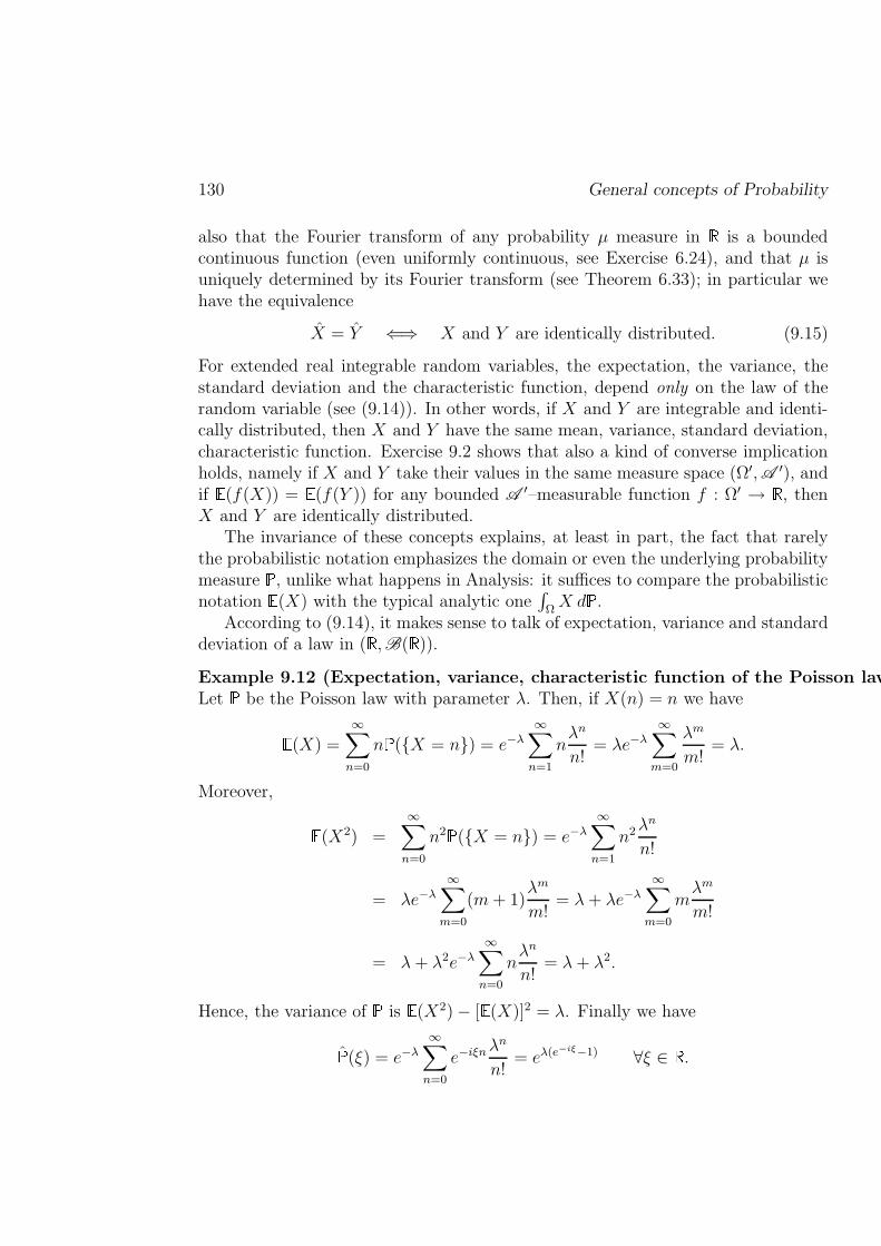
130 General concepts of Probability
also that the Fourier transform of any probability µ measure in
is a boundedcontinuous function (even uniformly continuous, see Exercise 6.24), and that µ isuniquely determined by its Fourier transform (see Theorem 6.33); in particular wehave the equivalence
X = Y ⇐⇒ X and Y are identically distributed. (9.15)
For extended real integrable random variables, the expectation, the variance, thestandard deviation and the characteristic function, depend only on the law of therandom variable (see (9.14)). In other words, if X and Y are integrable and identi-cally distributed, then X and Y have the same mean, variance, standard deviation,characteristic function. Exercise 9.2 shows that also a kind of converse implicationholds, namely if X and Y take their values in the same measure space (Ω′,A ′), andif
(f(X)) =
(f(Y )) for any bounded A ′–measurable function f : Ω′ →
, thenX and Y are identically distributed.
The invariance of these concepts explains, at least in part, the fact that rarelythe probabilistic notation emphasizes the domain or even the underlying probabilitymeasure
, unlike what happens in Analysis: it suffices to compare the probabilistic
notation
(X) with the typical analytic one
∫ΩX d
.
According to (9.14), it makes sense to talk of expectation, variance and standarddeviation of a law in (
,B(
)).
Example 9.12 (Expectation, variance, characteristic function of the Poisson law)Let
be the Poisson law with parameter λ. Then, if X(n) = n we have
(X) =
∞∑
n=0
n(X = n) = e−λ
∞∑
n=1
nλn
n!= λe−λ
∞∑
m=0
λm
m!= λ.
Moreover,(X2) =
∞∑
n=0
n2(X = n) = e−λ
∞∑
n=1
n2λn
n!
= λe−λ
∞∑
m=0
(m+ 1)λm
m!= λ+ λe−λ
∞∑
m=0
mλm
m!
= λ+ λ2e−λ
∞∑
n=0
nλn
n!= λ+ λ2.
Hence, the variance of
is
(X2) − [
(X)]2 = λ. Finally we have
ˆ(ξ) = e−λ
∞∑
n=0
e−iξnλn
n!= eλ(e−iξ−1) ∀ξ ∈
.
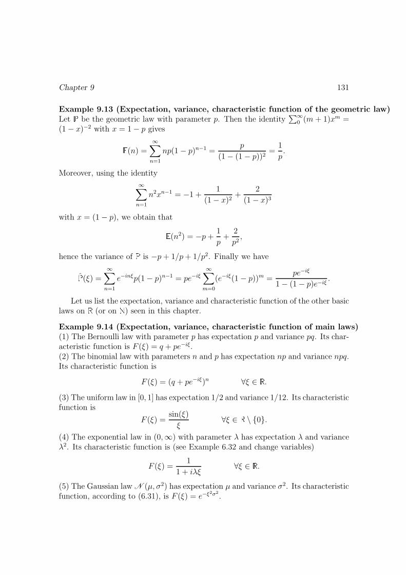
Chapter 9 131
Example 9.13 (Expectation, variance, characteristic function of the geometric law)Let
be the geometric law with parameter p. Then the identity
∑∞0 (m + 1)xm =
(1 − x)−2 with x = 1 − p gives(n) =
∞∑
n=1
np(1 − p)n−1 =p
(1 − (1 − p))2=
1
p.
Moreover, using the identity
∞∑
n=1
n2xn−1 = −1 +1
(1 − x)2+
2
(1 − x)3
with x = (1 − p), we obtain that(n2) = −p +
1
p+
2
p2,
hence the variance of
is −p + 1/p+ 1/p2. Finally we have
ˆ(ξ) =
∞∑
n=1
e−inξp(1 − p)n−1 = pe−iξ
∞∑
m=0
(e−iξ(1 − p))m =pe−iξ
1 − (1 − p)e−iξ.
Let us list the expectation, variance and characteristic function of the other basiclaws on
(or on
) seen in this chapter.
Example 9.14 (Expectation, variance, characteristic function of main laws)(1) The Bernoulli law with parameter p has expectation p and variance pq. Its char-acteristic function is F (ξ) = q + pe−iξ.(2) The binomial law with parameters n and p has expectation np and variance npq.Its characteristic function is
F (ξ) = (q + pe−iξ)n ∀ξ ∈ .
(3) The uniform law in [0, 1] has expectation 1/2 and variance 1/12. Its characteristicfunction is
F (ξ) =sin(ξ)
ξ∀ξ ∈ \ 0.
(4) The exponential law in (0,∞) with parameter λ has expectation λ and varianceλ2. Its characteristic function is (see Example 6.32 and change variables)
F (ξ) =1
1 + iλξ∀ξ ∈
.
(5) The Gaussian law N (µ, σ2) has expectation µ and variance σ2. Its characteristicfunction, according to (6.31), is F (ξ) = e−ξ2σ2
.
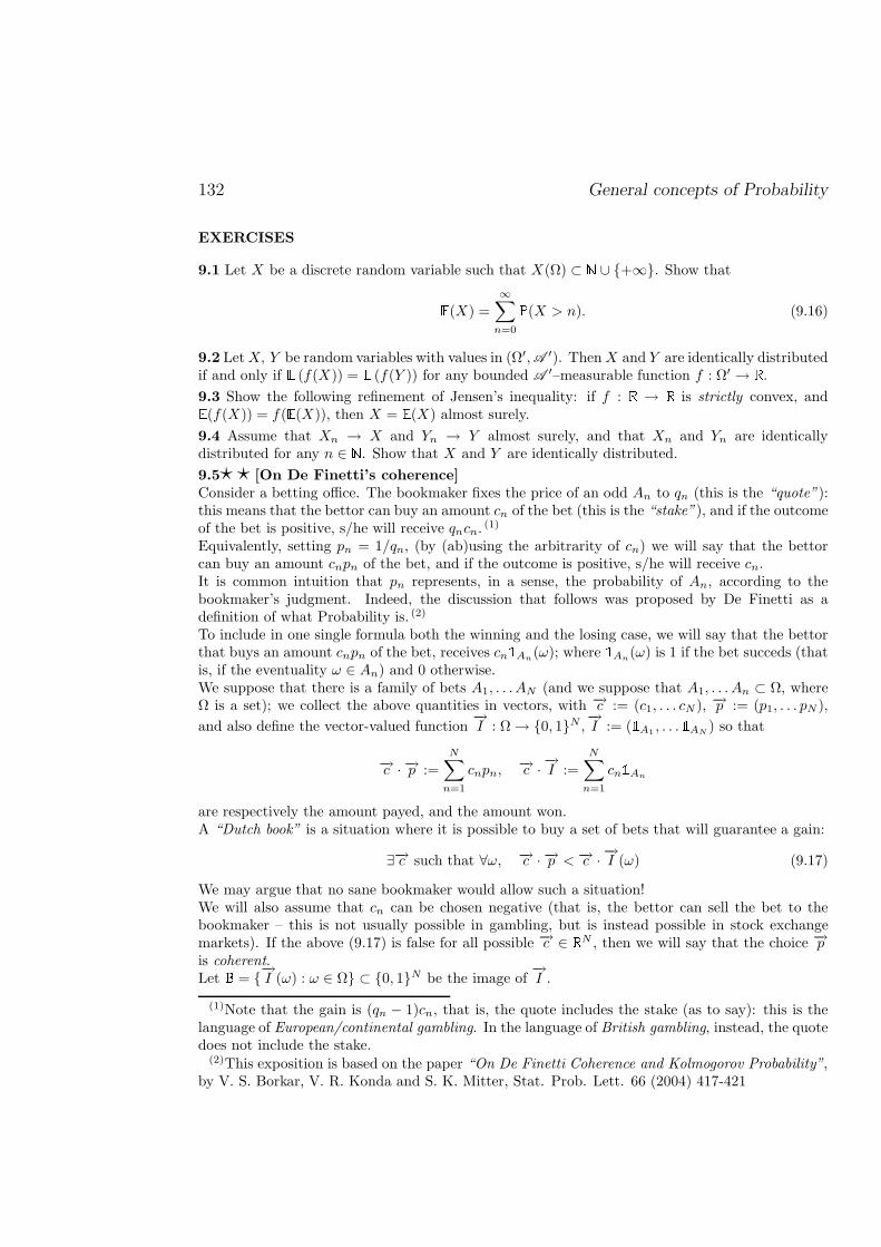
132 General concepts of Probability
EXERCISES
9.1 Let X be a discrete random variable such that X(Ω) ⊂ ∪ +∞. Show that
(X) =
∞∑
n=0
(X > n). (9.16)
9.2 LetX, Y be random variables with values in (Ω′,A ′). ThenX and Y are identically distributedif and only if (f(X)) = (f(Y )) for any bounded A ′–measurable function f : Ω′ → .
9.3 Show the following refinement of Jensen’s inequality: if f : → is strictly convex, and(f(X)) = f((X)), then X = (X) almost surely.
9.4 Assume that Xn → X and Yn → Y almost surely, and that Xn and Yn are identicallydistributed for any n ∈ . Show that X and Y are identically distributed.
9.5? ? [On De Finetti’s coherence]Consider a betting office. The bookmaker fixes the price of an odd An to qn (this is the “quote”):this means that the bettor can buy an amount cn of the bet (this is the “stake”), and if the outcomeof the bet is positive, s/he will receive qncn. (1)
Equivalently, setting pn = 1/qn, (by (ab)using the arbitrarity of cn) we will say that the bettorcan buy an amount cnpn of the bet, and if the outcome is positive, s/he will receive cn.It is common intuition that pn represents, in a sense, the probability of An, according to thebookmaker’s judgment. Indeed, the discussion that follows was proposed by De Finetti as adefinition of what Probability is. (2)
To include in one single formula both the winning and the losing case, we will say that the bettorthat buys an amount cnpn of the bet, receives cnAn
(ω); where An(ω) is 1 if the bet succeds (that
is, if the eventuality ω ∈ An) and 0 otherwise.We suppose that there is a family of bets A1, . . . AN (and we suppose that A1, . . . An ⊂ Ω, whereΩ is a set); we collect the above quantities in vectors, with −→c := (c1, . . . cN ), −→p := (p1, . . . pN ),
and also define the vector-valued function−→I : Ω → 0, 1N ,
−→I := (A1
, . . . AN) so that
−→c · −→p :=
N∑
n=1
cnpn,−→c · −→I :=
N∑
n=1
cnAn
are respectively the amount payed, and the amount won.A “Dutch book” is a situation where it is possible to buy a set of bets that will guarantee a gain:
∃−→c such that ∀ω, −→c · −→p < −→c · −→I (ω) (9.17)
We may argue that no sane bookmaker would allow such a situation!We will also assume that cn can be chosen negative (that is, the bettor can sell the bet to thebookmaker – this is not usually possible in gambling, but is instead possible in stock exchangemarkets). If the above (9.17) is false for all possible −→c ∈ N , then we will say that the choice −→pis coherent.Let = −→I (ω) : ω ∈ Ω ⊂ 0, 1N be the image of
−→I .
(1)Note that the gain is (qn − 1)cn, that is, the quote includes the stake (as to say): this is thelanguage of European/continental gambling. In the language of British gambling, instead, the quotedoes not include the stake.
(2)This exposition is based on the paper “On De Finetti Coherence and Kolmogorov Probability”,by V. S. Borkar, V. R. Konda and S. K. Mitter, Stat. Prob. Lett. 66 (2004) 417-421
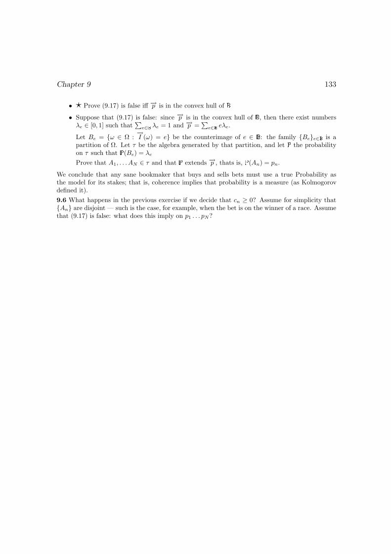
Chapter 9 133
• ? Prove (9.17) is false iff −→p is in the convex hull of
• Suppose that (9.17) is false: since −→p is in the convex hull of , then there exist numbersλe ∈ [0, 1] such that
∑e∈ λe = 1 and −→p =
∑e∈ eλe.
Let Be = ω ∈ Ω :−→I (ω) = e be the counterimage of e ∈ : the family Bee∈ is a
partition of Ω. Let τ be the algebra generated by that partition, and let the probabilityon τ such that (Be) = λe
Prove that A1, . . . AN ∈ τ and that extends −→p , thats is, (An) = pn.
We conclude that any sane bookmaker that buys and sells bets must use a true Probability asthe model for its stakes; that is, coherence implies that probability is a measure (as Kolmogorovdefined it).
9.6 What happens in the previous exercise if we decide that cn ≥ 0? Assume for simplicity thatAn are disjoint — such is the case, for example, when the bet is on the winner of a race. Assumethat (9.17) is false: what does this imply on p1 . . . pN?

134 General concepts of Probability
Chapter 10
Conditional probability andindependence
Let (Ω,A ,) be a probability space. Given two events A and B, with
(B) > 0,
the conditional probability(A∣∣B) of A given B is given by
(A∣∣B) :=
(A ∩ B)(B)
. (10.1)
Using a measure-theoretic notation,(·∣∣B) is the probability measure
B
/(B).
The notion of conditional probability is linked to the interpretation of probabilityas “quantitative evaluation of the possibility that an event occurs”; this evaluationhas to be based on the available informations. This is why the knowledge that theevent B occurred modifies the initial probability distribution
, and leads to the
conditional probability
B
/(B).
For instance, if Ω = 1, 2, 3, 4, 5, 6 is the canonical probability space associatedto the toss of a die, then
(6∣∣2, 4, 6
)=
1
3and
(6∣∣1, 3, 5
)= 0.
Or, if Ω = [0, 1] with the canonical probability structure, then
(x ≤ 1
3∣∣x ≤ 1
2)
=2
3.
Maybe the wrong identification between the concepts of probability and con-ditional probability is underlying all wrong beliefs about delayed numbers in lot-teries and similar games: if one randomly extracts 5 integer numbers between 1and 90 (re-inserting the 5 chosen numbers in the ballot-box after each extraction),
135
136 Conditional probability and independence
the probability that a given number, say 36, is not chosen in 100 extractions is(1 − 5/90)100 ∼ 3 · 10−3, but the conditional probability that it is not chosen in the100-th extraction, knowing that is has not been chosen in the first 99 extractions, is5/90 (this happens because this process has “no memory”, as we will see later on).
If one looks at probability as the limit of frequencies of succesful events, theformula (10.1) can be justified as follows: in a scheme of n trials we have
inn
∼ (A ∩ B) and
bnn
∼ (B),
where in, bn are respectively the number of times the events A ∩B, B occurred. Inorder to compute the conditional probability P (A
∣∣B) we consider, as it must be,only the fraction in/bn, ignoring the n − bn cases in which B did not occur. Then,multiplying and dividing by n we get
(A∣∣B) ∼ in
bn=inn
· nbn
∼(A ∩B)(B)
.
Notice also that if (B1, . . . , Bn) is a partition of Ω made by sets in A , then thefollowing Law of Total Probability holds:
(A) =
n∑
i=1
(Bi)
(A∣∣Bi). (10.2)
This is the identity used, more or less implicitly, in all exercises of discrete probabilityin which the probability of an event is computed by considering separately the casesA ∩ B1, . . . , A ∩Bn.
10.1 Independence of events, σ–algebras, random
variables
Two events A and B are said to be indipendent if(A∣∣B) =
(A), i.e. if
(A∩B) =
(A)
(B). Intuitively, A is independent of B if the probability of the occurrence of
A is not affected by the knowledge that B occurred. For instance, if Ω = H, Tn
is the canonical space associated to n-consecutive tosses of a coin, then
(ωn = T∣∣ωn−1 = H
)=
1
2and
(ωn = T∣∣ωn−1 = T
)=
1
2
because the events are independent. On the other hand, in the case of the toss of adie, the events 2 and 2, 4, 6 are clearly not independent.
More generally we can give the following definition:
Chapter10 137
Definition 10.1 (Independence for families of events) A family Aii∈I ⊂ Ais said to be independent if
(⋂
i∈J
Ai
)=∏
i∈J
(Ai)
for any finite set J ⊆ I.
In order to extend the concept of independence to families of random variableswe need the following definition. Let us be given a family, indexed by i ∈ I, ofrandom variables Xi : Ω → Ei, with (Ei, Ei) measurable spaces. For a fixed indexi ∈ I, the σ–algebra generated by Xi is
Gi :=X−1
i (A) : A ∈ Gi
;
note that this is the smallest σ-algebra in Ω which makes Xi (Gi − Ei)–measurable.Similarly, the σ–algebra generated by Xii∈I is the smallest σ-algebra G in Ω whichmakes all random variables Xi simultaneously (G − Ei)–measurable. G is the σ-algebra generated by the union
⋃i∈I Gi; if Fi is a family of generators of Ai (for
instance halflines, in the case Xi are real Borel variables), then G is the σ-algebragenerated by
X−1i (A) : A ∈ Fi, i ∈ I
.
Definition 10.2 (Independence for σ-algebras and random variables) A fam-ily Gii∈I of σ-algebras contained in A is said to be independent if
(⋂
i∈J
Ai
)=∏
i∈J
(Ai)
for any finite set J ⊆ I and any choice of Ai ∈ Gi, i ∈ J .A family of random variables Xii∈I is said to be independent if, denoting by
Gi the σ–algebra generated by each Xi, the family Gii∈I is independent.
Exercise 10.2 shows that also this concept can be formulated in terms of inde-pendence of pairs of events.
Notice also that a family of σ–algebras (or of random variables) is independentif and only if any finite subfamily is independent. Notice also that the concept ofindependence at the level of random variables does not require that the variables havethe same target: it requires, instead, that they are defined on the same probabilityspace (compare this with the concept of being identically distributed).
This is particularly evident in the following property:
138 Conditional probability and independence
Proposition 10.3 (Stability of independence under composition) Supposethat Xii∈I are independent, and Xi takes values in (Ei, Ei); let φi be measurablefunctions from (Ei, Ei) to (Di,Di); then the composite functions φi Xii∈I areindependent. Indeed, the σ–algebra generated by each φi Xi is a subset of theσ–algebra generated by each Xi.
We give now some important characterizations of the independence property forpairs or random variables taking their values respectively in the measurable spaces(E, E ) and (F,F ).
Proposition 10.4 The following properties are all equivalent to the independenceof X and Y :
(a)(X ∈ A ∩ Y ∈ B) =
(X ∈ A)(Y ∈ B) for A ∈ E ′ and B ∈
F ′, where E ′, F ′ are generators of E and F respectively, stable under finiteintersection;
(b) (f(X)g(Y )) =
(f(X))
(g(Y )) (10.3)
for any pair of functions f : E → , g : F →
, with f E –measurable and gF–measurable, and f, g either both bounded or both nonnegative;
(c) The law of the joint random variable Z = (X, Y ) : (Ω,A ) → (X × Y, E ×F )is the product of the laws of X and Y .
If (E, dE) and (F, dF ) are metric spaces and E , F are the corresponding Borelσ-algebras, we have a fourth equivalent property
(d)
(f(X)g(Y )) =
(f(X))
(g(Y )) for any pair of continuous functions f : E →
, g : F →
, with f, g either both bounded or both nonnegative;
Proof. The independence, in what follows denoted by (i), is equivalent to (a).Indeed, it suffices to notice that for B ∈ F ′ fixed, the collection of sets A ∈ Esatisfying
(X ∈ A ∩ Y ∈ B) =
(X ∈ A)(Y ∈ B) (10.4)
is a Dynkin class and contains E ′. Therefore, by the Dynkin theorem, this collectioncoincides with E . As a consequence, the collection of sets F ∈ F such that (10.4)holds for all E ∈ E contains F ′. Again, Dynkin theorem gives that this collectioncoincides with F .
We are now going to show that (i)⇒(b)⇒(c)⇒(i).(i)⇒(b). The formula is true for characteristic functions f =
A, g =
B (in this
case it reduces to (i)), hence for simple functions. Using Proposition 2.4 we obtain

Chapter10 139
its validity for nonnegative measurable functions. Eventually, splitting in positiveand negative part, it holds for bounded measurable functions.(b)⇒(c). Denoting by λ the law of Z, choosing f =
A and g =
B with A ∈ E and
B ∈ F , we get
λ(A× B) =
λ(
A×B) =
(Z1 ∈ A ∩ Z2 ∈ B)
=
(f(X)g(Y )) =
(f(X))
(g(Y )) = µ(A)ν(B),
with µ, ν respectively equal to the laws of X and Y . Hence λ = µ× ν.(c)⇒(i). Denoting by µ, ν the laws of X and Y respectively, we have
(X ∈ A ∩ Y ∈ B) =
(Z1 ∈ A ∩ Z2 ∈ B) = µ× ν(A×B)
= µ(A)ν(B) =(X ∈ A)(Y ∈ B).
Finally, it is clear that (b)⇒(d) if the σ-algebras in E and F are the Borel σ–algebras, as continuous functions are measurable. We then show that (d)⇒(a) wherewe set E ′ and F ′ to be respectively the open sets in E and F . Let then A ⊂ Eand B ⊂ F be open; by Exercise 2.9 we know that there exist two sequences ofnonnegative continuous functions fn : E → [0, 1] and gn : F → [0, 1] monotonicallyconverging to
A and
B: we then just pass to the limit into
(fn(X)gn(Y )) =
(fn(X))
(gn(Y )) to obtain, by monotone approximation, that
(
A(X)
B(Y )) =(
A(X))
(
B(Y )), that is(X ∈ A ∩ Y ∈ B) =
(X ∈ A)(Y ∈ B).
The above statement can be extended with no difficulty to the case of a familyof random variables Xi : Ω → Ei (indexed by a set I); all conditions are simplygeneralized, but with an interesting twist on condition (a) where we need the extracondition 3.
Proposition 10.5 The following properties are all equivalent to the independenceof the family (Xi)i∈I :
(a)
(⋂
i∈J
Xi ∈ Ai)
=∏
i∈J
(Xi ∈ Ai)
holds for any finite set J ⊆ I and any choice of Ai ∈ E ′i , i ∈ J .
Here, for any fixed i ∈ I, E ′i is a family satisfying
1. E ′i generates Ei
2. E ′i is stable under finite intersection
3. there exist at most countably many Bn ∈ E ′i such that
⋃nBn = Ei. (This
condition is obviously true in the simpler case when Ei ∈ E ′i ).
140 Conditional probability and independence
(b) ∏
i∈J
(fi(Xi)) =
(∏
i∈J
fi(Xi))
(10.5)
for any finite set J ⊆ I, for any choice of real Borel functions fi : Ei →,
either all bounded or all nonnegative;
(c) The law of the joint random variable Z = (Xi)i∈I : (Ω,A ) → (×i∈I Ei,×i∈I Ei)is the product of the laws of Xi.
If Ei are metric spaces and Ei are the corresponding Borel σ-algebras, we have afourth equivalent property
(d) equality (10.5) holds for any finite set J ⊆ I, for any choice of real continuousfunctions fi : Ei →
, either all bounded or all nonnegative.
We omit the proof, that is a straightforward generalization of the previous one.
The above two propositions have many interesting corollaries:
Corollary 10.6 Suppose X1, · · ·Xn : Ω → C are discrete random variables takingvalues in a countable set C; and suppose that for all choices of x1, . . . , xn ∈ C,
(n⋂
i=1
Xi = xi)
=
n∏
i=1
(Xi = xi)
then X1, · · ·Xn are independent. The proof follows from (a), choosing E ′i to be the
family of singletons of C.
The above can also be proved as in Exercise 10.11.
Corollary 10.7 Given Aii∈I ⊂ A , the following are equivalent:
• the family Aii∈I is independent, as defined in 10.1
• the family of characteristic functions Aii∈I is independent, as defined in
10.2
The proof again follows from (a), choosing Ei = P0, 1 and E ′i = 1, 0, 1.
We add another important independence criterion, that will be useful in thefollowing.
Proposition 10.8 (Recursive independence criterion) Let (Xn) be a sequenceof random variables such that, for any n ≥ 1, Xn is independent from (X0, . . . , Xn−1).Then (Xn) is an independent sequence.
Chapter10 141
Proof. Let 0 ≤ i1 < i2 < · · · < ik and Aj = X−1ij
(Bj) be in the σ–algebragenerated by Xij , j = 1, . . . , k. Setting n = ik, the event An is independent fromthe event ∩j<kAij , as the former belongs to the σ–algebra generated by Xn and thelatter to the σ–algebra generated by (X0, . . . , Xn−1). We have then
(k⋂
j=1
Aij
)=
(k−1⋂
j=1
Aij
)· (Aik).
Continuing in this way we get(∩k
1Aij ) =∏k
1
(Aij ).
By combining the above ideas, it is possible to create many other “independencecriterions”; see in Exercises 10.1. . . 10.4; but not all of them work, as seen in Exercise10.5.
10.1.1 Indipendence of real valued variables
Whenever X and Y are real valued and integrable we can obtain from 10.4(b),splitting X and Y in positive and negative part, and using the independence of thepairs (X+, Y +), (X+, Y −), (X−, Y +), (X−, Y −), that XY is integrable and
(XY ) =
(X)
(Y ). (10.6)
In this identity the independence is really crucial: without this assumption we cansay that XY is integrable only if X and Y are square integrable, and typically(XY ) 6=
(X)
(Y )! An analogous splitting in real and immaginary part shows
that (10.6) still holds for integrable complex-valued random variables X, Y .
The identity (10.6) has a remarkable consequence: if X1, . . . , Xn are pairwiseindependent, then they are scorrelated, so that the variance of the sum X1+ · · ·+Xn
is the sum of the variances of the Xi. Indeed, as Xi−ci is still independent of Xj−cjwhen i 6= j and ci, cj ∈
, in the proof of this fact we can assume with no loss ofgenerality that the Xi are centered. Then, we have
σ2(X1 + · · ·+Xn) =
(|X1 + · · ·+Xn|2) =
n∑
i, j=1
(XiXj) (10.7)
=
n∑
i=1
(X2
i ) =
n∑
i=1
σ2(Xi).
This fact shows that the variance of the arithmetic mean of the Xi can be estimatedby C/n, if all variances of Xi are bounded by C. This fact will be the basis of theproof of the strong law of large numbers, in the next chapter.
142 Conditional probability and independence
At the same time it is important to remark that any family of random variablesmay be “independent” whereas only real (or, vector valued) random variables maybe “scorrelated”.
If moreover (X1, . . . , Xn) are real integrable and independent, then (applyingequation (10.5) with fi(x) = |x|) we obtain that their product
∏nj=1Xj is integrable;
by Exercise 10.7, the product X1 · · ·Xn−1 is independent from Xn; using this factwe can repeatedly apply (10.6) to obtain
( n∏
j=1
Xj
)=
n∏
j=1
(Xj) (10.8)
Again, an analogous argument holds for integrable complex-valued random variables.
Example 10.9 Using the independence of∑n−1
i=1 Xi of Xn we can check that therandom variable Sn =
∑ni=1Xi in Example 9.4 has binomial law with parameters n
and p. We can show that
(Sn = i) =
(ni
)piqn−i ∀1 ≤ i ≤ n
by induction on n using the fact that Sn−1 is independent of Xn and (10.2):(Sn = i) = q
(Sn = i∣∣Xn = 0
)+ p
(Sn = i∣∣Xn = 1
)
= q (Sn−1 = i
∣∣Xn = 0)
+ p (Sn−1 = i− 1
∣∣Xn = 1)
=
(n− 1
i
)piqn−1−i · q +
(n− 1
i− 1
)pi−1qn−1−i+1 · p =
(ni
)piqn−1.
We now show a basic rule for computing the characteristic function of the sumof n independent random variables.
Proposition 10.10 If Y1, . . . , Yn are independent random variables, then
n∑
j=1
Yj =n∏
j=1
Yj.
Proof. For any ξ ∈ we have
n∑
j=1
Yj(ξ) =
(e−iξ
nP
j=1Yj
)=
(
n∏
j=1
e−iξYj),
whileYj(ξ) =
(e−iξYj), 1 ≤ j ≤ n.
The conclusion follows by (10.8) with Xj = e−iξYj , noticing that (Xj) are stillindependent.
Chapter10 143
10.2 Independent sequences with prescribed laws
A sequence of random variables (Xi) all taking values in the same space E, E iscalled a discrete stochastic process. Here “discrete” refers to the fact that the indexi varies in
, while in many other important applications also continuous paramaters
are used (typically Xt, with t ∈ ).
One of the most important applications of Proposition 10.4 consists in the pos-sibility of building, given a sequence (
i) of laws in the measurable spaces (Ω′
i,A′i ),
an independent sequence (Xi) of random variables with values in Ω′i and having laws
i. In many cases the law
i = µ does not depend on i; in this case we will say that
the sequence (Xi) is independent and identically distributed.In order to build a probability space and independent mapsXi with this property,
it suffices to take as probability space
(Ω,A ,) :=
(∞∏
i=1
Ω′i,
∞×i=1
Ai,∞×i=1
i
),
and as functions Xi(ω) the canonical projections on the i-th coordinate, i.e. Xi(ω) =ωi. As, by the definition of product measure
(Xi ∈ Ai) =
(ω : ωi ∈ Ai) =
i(Ai) ∀Ai ∈ Ai,
we obtain that the law of Xi is µi. More generally, an analogous argument givesthat the law of (Xi1, . . . , Xin) is µi1 × · · · × µin, because for any choice of Ak ∈ Aik ,1 ≤ k ≤ n, the event
ω ∈ Ω : wij ∈ Aij j = 1, . . . , k
is cylindrical and has-probability
k∏
j=1
ij (Aij ) =
n×j=1
µij(Ai1 × · · · × Ain).
The independence (not only pairwise, but as a whole) of the variables Xi follows byProposition 10.5(c).
We begin with a fundamental example, that can be built as a product of infinitecopies of the Bernoulli law (as in 9.2.(3))
Example 10.11 (Bernoulli process) A discrete Bernoulli process with parame-ter p ∈ [0, 1] is a sequence of independent and identically distributed random vari-ables Xi with Bernoulli law with parameter p.
144 Conditional probability and independence
Given a discrete stochastic process (Xn), one can typically build many newrandom variables starting from Xn, as shown in the following example.
Example 10.12 (k-success time and Pascal laws) We consider a discrete Bernoulliprocess with parameter p. We consider the random variable
T (ω) := inf n ≥ 1 : Xn(ω) = 1 ,
so that T represents the time of the first success. As T > n is the intersection ofthe sets Xi = 0 for i = 1, . . . , n, the independence of (Xn) gives
(T > n) = (1 − p)n.
In particular one has that almost surely T is finite. Moreover, writing T = n =T > n− 1 \ T > n, we get
(T = n) = p(1 − p)n−1 ∀n ≥ 1.
This shows that T has a geometric law with parameter p, so that
(T ) = 1/p. We
have also
(T − n = k∣∣T > n
)=
(T = n + k)(T > n) =
(T = k), (10.9)
therefore the law of T − n, conditioned to T > n, has still geometric law withparameter p (one says that the geometric law has no memory).
Let us build now new random variables as follows: T1 = T ,
T2(ω) := min n > T1(ω) : Xn(ω) = 1
and, recursively, Tk+1(ω) := min n > Tk(ω) : Xn(ω) = 1. The variables Tk repre-sent the time of the k-th success. Let us compute the law of Tk, called Pascal lawof parameter p, k: since for n ≥ k we have
Tk = n = Xn = 1 ∩ X1 + · · ·+Xn−1 = k − 1
we get
(Tk = n) = p ·
(n− 1
k − 1
)pk−1(1 − p)n−1−(k−1)
=
(n− 1
k − 1
)pk(1 − p)n−k n = k, k + 1, . . .
Let eventually U1 = T1 and Un+1 = Tn+1 − Tn be the times of returning tosuccess : then the sequence (Un)n is a sequence of independent geometrical randomvariables. (The proof follows from exercise 10.1).
Chapter10 145
A very particular but interesting case of the previous construction correspondsto the situation when (Ω′
i,A′
i ) = (−1, 1,P(−1, 1)) and the laws
i are all equalto µ = (δ−1 + δ1)/2.
Example 10.13 (Rademacher sequence) Let
(Ω,A ,) :=
([0, 1],B([0, 1]),L 1
)
and let us divide [0, 1] in 2n closed intervals with length 2−n, setting Rn alternativelyequal to −1 and 1 in the interior of these intervals, defining Rn on the extreme pointsof the intervals in such a way that Rn is right continuous (other choices are possible,without changing the law of Rn). The law of Rn is µ because
(Rn = ±1) =
1
2.
We will check that (Rn) is independent in two ways, a direct one and a moretheoretical one. Thanks to the recursive independence criterion 10.8 it suffices tocheck that for any n the σ–algebra generated by Rn+1 is independent of the σ–algebra generated by R1, . . . , Rn. The latter σ–algebra is generated by intervals Iwith length 2−n on which each Rn+1 is equal to −1 in the first half, and equal to 1in the second half (the values in the mid points are irrelevant), hence
(Rn+1 = ±1∣∣I)
=
(Rn+1 = ±1 ∩ I)
(I)
= 2−n−1+n =(Rn+1 = ±1).
This proves that Rn+1 is independent of the σ–algebra generated by R1, . . . , Rn.Another way to show the independence is to notice that Rn = (2Xn − 1) φ,
where
φ : ([0, 1],B([0, 1])) →(
∞∏
i=1
0, 1,∞×i=1
P(0, 1))
is the map associating to any number in [0, 1] its binay expansion (in case of non-uniqueness one can choose the one with finitely many digits equal to 1) and Xn isthe map that to ω ∈ ∏∞
1 0, 1 associates its i-th coordinate. Notice also that φ
maps the uniform measure in [0, 1] in the product measure
=×∞
1 (δ0 + δ1)/2 (seeExercise 8.2). Being the sequence Yn = 2Xn − 1 independent, we have
L 1
(n⋂
j=1
R−1ij
(Aij)
)= L 1
(φ−1(
n⋂
j=1
Y −1ij
(Aij ))
)=
(n⋂
j=1
Y −1ij
(Aij )
)
=
n∏
j=1
(Y −1
ij(Aij )) =
n∏
j=1
L 1(φ−1(Y −1ij
(Aij )))
=n∏
j=1
L 1(R−1ij
(Aij ))
146 Conditional probability and independence
for any choice of 1 ≤ i1 < i2 · · · < in and Aij ⊆ −1, 1.
The Rademacher sequence provides us with a simple example of a family ofrandom variables pairwise independent but not globally independent: it suffices toconsider the triplet of functions (R1, R2, R1R2); where this triplet independent, wewould obtain thanks to Exercise 10.7 that R1R2 is independent from itself, and thisis clearly false (see also Exercise 10.8). On the other hand, it is easy to check thatthe pairs (R1, R1R2) and (R2, R1R2) are independent.
From that example we can easily generate another important example: a processof random variables that are pairwise independent but not all independent; to thisend. let
3 be the law of (R1, R2, R1R2), and use the construction shown at the
beginning of the section once again, to build infinite variables that have law
3 andare independent.
EXERCISES
10.1[Recursive discrete independence criterion] Let (Xn)n be a sequence of discrete randomvariables taking values in a countable set C; suppose that, for any n ≥ 1, for all choices ofx0, . . . , xn+1 ∈ C, letting B =
⋂ni=0Xi = xi,
(Xn+1 = xn+1 | B) = (Xn+1 = xn+1)
whenever (B) > 0. Then (Xn)n∈ is an independent sequence.
10.2 (Independence is assured if we ask that any choice of disjoint subfamilies be independent.) Show thatXii∈I is independent if and only if, chosen J, K ⊂ I disjoint and denoting by AI and AK theσ–algebras generated by Xii∈J and Xii∈K , we have
(A ∩B) = (A)(B) ∀A ∈ AJ , B ∈ AK .
10.3 (Independence is still assured if we only assume that each variable is independent from all the others.)
Show that Xii∈I is independent if and only if, for any chosen j ∈ I, denoting by Aj and A¬j
the σ–algebras generated by Xj and (Xi)i6=j , we have
(A ∩B) = (A)(B) ∀A ∈ Aj, B ∈ A¬j .
10.4 (In the case of events, we can test independence of one event w.r.t. a finite sub family of all the others.)
Suppose that Xi takes values in 0, 1. Show that Xii∈I is independent if and only if, for anychosen j ∈ I and K ⊂ I finite and with j 6∈ K, defining A = Xj = 1, B = Xi = 1, i ∈ K, wehave
(A ∩B) = (A)(B).
(Hint: Xi = Ciwith Ci ∈ A ; so A = Cj and B =
⋂i∈K Ci; by 10.7, show that the event Cii∈I
are independent).
Note that in the Exercise 10.2 we test independence of each Xj against the block (Xi)i∈K where K = i : i 6= j;
whereas in 10.4 we consider more generally all choices j, K ⊂ I where j 6∈ K. The following example shows that
we cannot generalize 10.4 further, that is, supposing that(A ∩ B) =
(A)
(B) holds only when K = i : i 6= j.
Chapter10 147
10.5 Show that there exists an example of 3 variables (X1, X2, X3) taking values in 0, 1, suchthat (X1, X2, X3) are not independent, but, for any chosen j ∈ 1, 2, 3 and defining A = Xj = 1,B = Xi = 1, i 6= j, they satisfy
(A ∩B) = (A)(B).
(Hint: let V be the set of all possible densities p ∈ 8 of the law of (X1, X2, X3) on 0, 13 that satisfy the requisite;
prove that V is a smooth manifold of dimension 4 in a neighbourhood of (1/8, 1/8 . . . , 1/8); whereas the space of
all densities of independent variables is at most 3 dimensional.)
10.6(Ricomposition of independence) Let (Xi)i∈J be a family of random variables. Let J bea partition of J in non empty subsets; for I ∈ J let YI = (Xi)i∈I be the vector random variable;suppose that,
• for any I ∈ J , the family (Xi) with i ∈ I is a family of independent random variables
• the family of variables YI , for I ∈ J , is a family of independent random variables
Prove that (Xi)i∈J is a family of independent random variables.
Find simple examples where (Xi)i∈J is not a family of independent random variables, but one ofthe two properties above holds.
10.7 Assume that X1, . . . , Xn+1 are real-valued independent random variables. Then, for anyBorel function f : n → the random variables
f(X1, . . . , Xn) and Xn+1
are independent. Hint: Let Y = (X1, . . . , Xn), use exercises 10.6 and Prop. 10.3.
10.8 Show that a real Borel random variable X is independent of itself if and only if X is almostsurely equal to a constant.
Note also that a random variable X almost surely equal to a constant, is independent of any otherrandom variable.
10.9 Find an example of a random variable X that is independent of itself but not almost surelyequal to a constant.
(Hint: find a σ-algebra τ on such that x ∈ τ, ∀x ∈ , and find a probability on (, τ) suchthat x = 0 and (A) ∈ 0, 1, ∀A ∈ τ ; let X : (, τ, ) → (, τ) be the identity.)
10.10 Suppose that X,Y are two real independent random variables, and X − Y is a.s. constant:prove that X and Y are a.s. constant.
10.11(Density and independence) Let X1, . . . , Xn be random variables on (Ω,F , ) withvalues in a space (C,C , µ); let νi := X# be the law of Xi; suppose that νi µ; let ρi ∈L1(Ω,F , ) be the density of νi w.r.t. µ (as defined by the Radon–Nikodym Theorem 6.12). LetY = [X1, . . . , Xn] be the block random variables with values in a space (Cn,C n) let ν = Y# andµ = µn. Prove that these two are equivalent
• X1, . . . , Xn are independent
• ν µ, and
ρ(x) = ρ1(x1) · · · ρn(xn) for µ almost all x ∈ Cn
where ρ is the density of ν w.r.t. µ, and x = (x1, . . . xn) ∈ Cn.
148 Conditional probability and independence
The above is often applied to the case of discrete variables (when C is finite or countable): supposethat µ is the counting measure, then any measure on C is absolutely continuous w.r.t. to µ; inthat case, the marginal density satisfies
Xi ∈ A =∑
xi∈A
ρi(x)
for any A ∈ C; and the block satisfies
[X1 . . . , Xn] ∈ B =∑
x∈B
ρ1(x1) · · · ρn(xn) ∀B ⊂ Cn
if and only if X1, . . . , Xn are independent.
10.12? Let µ, ν be probability measures in . Show that the convolution µ∗ν of µ and ν, definedby
µ ∗ ν(A) :=
∫
∫A(x + y) dµ(x) dν(y) A ∈ B()
is a probability measure in . Show that ∗ is a commutative and associative product among theprobability measures in , and find the identity element of this product. Show that
∫f(z)d(µ ∗ ν)(z) =
∫
∫f(x+ y) dµ(x) dν(y)
for any Borel bounded function f : → .
10.13? Using Fubini–Tonelli theorem show that the law of the sum of two real independentvariables X , Y is given by µ ∗ ν, where µ is the law of X and ν is the law of Y .
10.14 Let (Xn)n∈ be a Bernoully process of parameter p ∈ (0, 1); let T (ω) := inf n ≥ 0 : Xn(ω) = 1be the first success (starting from n = 0); let Y := XT+1: compute Y = 1 and Y = 1 | Xn =110.15 Show that the geometric law is the only law with values in such that the “no memory”property (10.9) holds. (See in example 10.12 for more details).
10.16 We recall (from page ??) that, given λ > 0, the exponential law with parameter λ is theprobability law on [0,∞) defined by E (λ) = 1
λ e−t/λL 1.
Let X be a real Borel random variable, positive almost surely. Let µ = X# be the law, supposethat it is supported in [0,∞), and absolutely continuous w.r.t. Lebesgue measure. Show that thethree following facts are equivalent:
• µ = E (λ) for a λ > 0
• (X > a+ b
∣∣X > a)
= (X > b) ∀a, b ≥ 0.
• there is a λ > 0 such that ∀t > 0, defining Qt(·) = (·|X > t)
λ = Qt(X − t) :=
∫(X(ω) − t) dQt(ω)
The second condition above means that exponential law has no memory (it is then the “continuousequivalent” of the geometric law; see the previous exercise).
Chapter 11
Convergence of random variables
In this chapter we will study and compare various concepts of convergence for se-quences of random variables: the almost sure convergence, the Lp convergence, al-ready seen in the measure-theoretic part of this book, the convergence in probabilityand finally the convergence in law.
We are given a probability space (Ω,A ,), a sequence of extended real random
variables (Xn) and a random variable X on (Ω,A ,). Let p ∈ [1,∞). We recall
thatlim
n→∞Xn = X in Lp(Ω,A ,
)
if Xn, X ∈ Lp(Ω,A ,) and
limn→∞
(|X −Xn|p) = 0.
11.1 Convergence in probability
We say that a sequence (Xn) of extended real random variables converges in prob-ability to X if for all δ > 0 we have (with the convention (+∞) − (+∞) = 0,(−∞) − (−∞) = 0)
limn→∞
(|X −Xn| > δ) = 0. (11.1)
Condition (11.1) is equivalent to the following one
∀ε > 0, ∃ nε ∈
such that(|X −Xn| > ε) < ε, ∀ n ≥ nε. (11.2)
Indeed, assume that (11.2) holds and fix δ > 0. Then by (11.2) it follows that forany integer k ≥ 1 there exists nk ∈
such that
n ≥ nk =⇒ (|X −Xn| > 1/k) <
1
k. (11.3)
149
150 Convergence of random variables
Since |X −Xn| > 1/k ⊃ |X −Xn| > δ for k > 1/δ, by (11.3) it follows that
n ≥ maxnk,1
δ =⇒
(|X −Xn| > δ) < 1
k.
Therefore(|X −Xn| > δ) → 0 as n → ∞. The converse implication is obvious,
just taking δ = ε and using the definition of the limit.The characterization (11.2) of convergence in probability suggests the introduc-
tion of the following distance
d(X, Y ) = inf δ > 0 :(|X − Y | > δ) < δ . (11.4)
The distance d is well defined, and obviously d(X, Y ) ≤ 1, because(|X − Y | >
δ) < δ for any δ > 1. Notice also that, by monotonicity
(|X − Y | > δ) < δ ∀δ > d(X, Y ). (11.5)
We will prove that d induces a distance in the class X (Ω) of equivalence classes ofextended real random variables in (Ω,A ,
). Here the equivalence relation is the
one induced by the almost sure coincidence, i.e.
X ∼ Y ⇐⇒ X = Y almost surely.
In the following we shall for simplicity identify (as we did in the first part of thebook) elements of X (Ω) with the corresponding equivalence classes, whenever thestatement does not depend on the choice of a particular representative.
Proposition 11.1 The space (X (Ω), d) is a metric space and the convergence in(X (Ω), d) coincides with the convergence in probability.
Proof. It is not hard to check that the function d defined in (11.4) is a distanceon equivalence classes: the symmetry property and the fact that d(X, Y ) = 0 if andonly if X = Y almost surely are straightforward, while the triangle inequality canbe proved by the following argument: if δ1 > d(X, Y ) and δ2 > d(Y, Z) then (11.5)gives
(|X − Y | > δ1) < δ1 and
(|Y − Z| > δ2) < δ2
and the inclusion |X − Z| > δ1 + δ2 ⊂ |X − Y | > δ1 ∪ |Y − Z| > δ2 gives
(|X − Z| > δ1 + δ2) < δ1 + δ2,
so that d(Y, Z) ≤ δ1 + δ2. Letting δ1 ↓ d(X, Y ), δ2 ↓ d(Y, Z) we obtain the triangleinequality.The definition of d implies that
(|Xn−X| > δ)(|Xn−X| > ε) < ε as soon as
Chapter11 151
d(Xn, X) < ε and ε < δ. Hence, convergence in (X (Ω), d) implies convergence inmeasure. Conversely, if Xn → X in measure and δ > 0, then
(|Xn−X| > δ) < δ
for n large enough, hence d(Xn, X) ≤ δ for n large enough. This proves thatd(Xn, X) → 0.
In the following theorem we collect the relations between almost sure conver-gence, convergence in Lp and convergence in probability.
Theorem 11.2 Let (Xn), X be extended real random variables. Then:
(i) if (Xn) converges to X almost surely, then (Xn) converges to X in probability.Conversely, if (Xn) converges to X in probability, there exists a subsequence(Xn(k)) converging to X almost surely.
(ii) if Xn, X ∈ Lp(Ω,A , µ) for some p ∈ [1,∞), then convergence of (Xn) to Xin Lp(Ω,A , µ) implies convergence in probability. The converse implicationholds only if |Xn|p are
–uniformly integrable.
Proof. (i) If Xn → X almost surely, then|Xn−X|>δ → 0 almost surely for all
δ > 0. Therefore its expectation, i.e. the probability of |Xn −X| > δ, tends to 0.Assume now that Xn → X in probability. For any integer k ≥ 1 we can find aninteger n(k) such that
(|Xn(k) −X| > 1
k) < 2−k,
because(|Xn − X| > 1/k) < 2−k for n large enough. For the same reason, we
can also choose recursively n(k) with the property above and in such a way thatn(k) > n(k − 1). For any δ > 0 we have |Xn(k) −X| > δ ⊂ |Xn(k) −X| > 1/kfor k ≥ 1/δ, hence
∞∑
k=1
(|Xn(k) −X| > δ) <∞ ∀δ > 0.
According to Borel-Cantelli Lemma 1.9, this implies that the lim supk|Xn(k)−X| >δ is
–negligible for any δ > 0. This means that Xn(k) → X almost surely.
(ii) If Xn → X in Lp(Ω,A , µ), then Markov’s inequality (9.4) gives
(|Xn −X| > δ) ≤ 1
δp
(|Xn −X|p)
and therefore Xn → X in probability. Conversely, assume that Xn → X almostsurely, and that |Xn|p are
-uniformly integrable. If, by contradiction, Xn do not
converge to X in Lp(Ω,A ,), we can find ε > 0 and a subsequence n(k) such that
(|Xn(k) −X|p) ≥ ε ∀k ∈ .
152 Convergence of random variables
But, on any subsequence Xn(k(l)) extracted from Xn(k) and converging almost surelyto X, we can apply Vitali’s convergence Theorem 2.16 to obtain that
(|Xn(k(l)) −
X|p) → 0 as l → ∞. This contradicts the previous inequality with k = k(l).
We have already seen in Remark 3.2 and Example 3.11 that the statements inTheorem 11.2 are optimal: there exist sequences converging in measure (even in anyLp with p < ∞) that are not converging almost surely, and there exist sequencesconverging almost surely but not in L1.
11.2 Convergence in law
We say that a sequence of real random variables (Xn) converges in law to a realrandom variable X if the probability measures (Xn)#
in
converge weakly to
X#
. Recall that, according to the very definition of convergence for laws on the
real line given in Definition 6.22, this means
limn→∞
(Xn)#
((−∞, x]) = X#
((−∞, x])
with at most countably many exceptions x, and so
limn→∞
(Xn ≤ x) =
(X ≤ x) (11.6)
with at most countably many exceptions x. Moreover, from Theorem 6.25 we deducethat:
Theorem 11.3 (Xn) is convergent in law to X if and only if
limn→∞
∫
ϕ(x) d(Xn)#
(x) =
∫
ϕ(x)X#
(x) ∀ϕ ∈ Cb(
),
or, equivalently (by the change of variables formula),
limn→∞
(ϕ(Xn)) =
(ϕ(X)) ∀ϕ ∈ Cb(
). (11.7)
Convergence in law is a very weak convergence that does not take at all intoaccount the pointwise behaviour of Xn and X (for instance, if Xn → X in lawand Y has the same law of X, then obviously Xn → Y in law). In particular,choosing identically distributed X and Y , with X 6= Y almost surely, one sees thatconvergence of Xn to X in law can’t imply any form of almost sure convergence ofXn (or in probability). We are going to show that convergence in probability impliesconvergence in law and that the converse implication holds only when the previousconstruction is impossible, i.e. when the law of X is a Dirac mass.
Chapter11 153
Proposition 11.4 If Xn → X in probability then Xn → X in law.
Proof. Let ϕ ∈ Cb(). If Xn → X almost surely, then ϕ(Xn) → ϕ(X) almost surely
and the dominated convergence theorem gives that (11.7) holds. In the general casewhen Xn → X in probability, assume by contradiction that
(ϕ(Xn)) does not
converge to
(ϕ(X)): then, we can find ε > 0 and a subsequence n(k) such that
∣∣(Xn(k)) −
(X)
∣∣ ≥ ε ∀k ∈ .
But, on any subsequence Xn(k(l)) extracted fromXn(k) converging almost surely toX,we already proved that
(Xn(k(l))) converges to
(X). This contradicts the previous
inequality with k = k(l).
Proposition 11.5 Assume that (Xn) converges in law to a constant c. Then (Xn)converges to c in probability.
Proof. Obviously the law of the constant random variable c is δc, whose distributionfunction is
Fc(x) =
1 if x ≤ c0 if x > c.
It is enough to show that(|Xn − X| > δ) → 0 for any δ > 0 such that the
convergence of the distribution functions of the laws ofXn to Fc occurs with x = c+δand x = c− δ. Since for any random variable Y we have
(|Y − c| > δ) =
(Y > δ + c) +
(Y < −δ + c)
≤ 1 − (Y ≤ δ + c) +
(Y ≤ −δ + c)
we obtain
limn→∞
(|Xn − c| > δ) ≤ 1 + lim
n→∞−
(Xn ≤ δ + c) +(Xn ≤ −δ + c)
= 1 − 1 + 0 = 0.
Finally, recalling that weak convergence of probability measures can be character-ized in terms of pointwise convergence of the Fourier transforms (see Theorem 6.35),we get:
Theorem 11.6 Let Xn, X be real random variables. Then Xn → X in law if andonly if Xn(ξ) → X(ξ) for all ξ ∈
.
154 Convergence of random variables
EXERCISES
11.1 Show that Xn → X in probability if, and inly if, (min1, ‖Xn −X‖) → 0 as n→ ∞.
11.2 Show that convergence in probability of real random variables is invariant under compositionwith continuous maps, namely Xn → X in probability implies ϕ(Xn) → ϕ(X) in probabilitywhenever ϕ : → is continuous. Hint: first consider the case when ϕ is uniformly continuous.
11.3? Show that (X (Ω), d) is a complete metric space. Hint: given a Cauchy sequence (Xn), itsuffices to show that a chosen subsequence (Xn(k)) satisfying
∞∑
k=0
d(Xn(k+1), Xn(k)) <∞
converges to some X ∈ X (Ω). To show the convergence of (Xn(k)), use Lemma 1.9 (as in theproof of Theorem 11.2(i)) to show that (Xn(k)(ω)) is a Cauchy sequence in almost surely.
Chapter 12
Sequences of independentvariables
12.1 Sequences of independent events
In this section we study the case of a sequence of characteristic functions, i.e. asequence of events. We will see that, in the case when the events are indepen-dent, a deterministic behaviour arises in the limit. This phenomenon is known asKolmogorov’s dichotomy. The results of this section will be used to study, moregenerally, independent sequences of random variables.
Lemma 12.1 (Borel–Cantelli) Let (An) be a sequence of independent events.Then
∞∑
n=0
(An) <∞ ⇐⇒
(lim supn→∞
An) = 0.
Proof. The proof of the implication ⇒ does not rely on independence, and itwas already mentioned in Chapter 1; let us recall its simple proof:
(
lim supn→∞
An
)= lim
p→∞
(∞⋃
n=p
An
)≤ lim
p→∞
∞∑
n=p
(An) = 0.
Conversely, for any p ∈ we have
(Ω \
∞⋃
n=p
An
)=
(∞⋂
n=p
(Ω \ An)
)=
∞∏
n=p
(1 − (An)) .
Taking limits as p→ ∞ we get
limp→∞
∞∏
n=p
(1 − (An)) = 1.
155
156 Sequences of independent variables
Choosing p0 such that the infinite product∏∞
p0(1−
(An)) is strictly positive, fromthe inequality (1 − x) ≤ exp(−x) we infer
exp
(−
∞∑
n=p0
(An)
)> 0.
Therefore the series∑
n
(An) converges.
From the Borel-Cantelli lemma we obtain the implication
∞∑
n=0
(An) = ∞ =⇒
(lim supn→∞
An) > 0. (12.1)
Actually, using Kolmogorov’s dicothomy, we have the much stronger implication
∞∑
n=0
(An) = ∞ =⇒
(lim supn→∞
An) = 1. (12.2)
In order to justify (12.2) and state the Kolmogorov’s dichotomy we need to statesome preliminary definitions. Given a sequence of σ-algebras An ⊆ A , we denoteby A∞, the terminal σ–algebra of the family: it is defined by ∩nBn, where Bn ⊆ Ais the σ–algebra generated by
∞⋃
i=n
Ai.
For instance, if (Xn) is an independent sequence of random variables and An arethe σ-algebras generated by Xn, then events of the form
lim supn→∞
An, An ∈ An; A :=
ω ∈ Ω :
∞∑
n=0
Xn(ω) converges
(12.3)
are terminal, while events of the form
ω ∈ A :
∞∑
n=0
Xn(ω) > 1
typically are not.Kolmogorov’s dichotomy is the first example of an important phenomenon: the
appearance of a deterministic behaviour from the superposition of many randomevents. Similar phenomena will be investigated in the law of large numbers and inergodic theorems.
Chapter12 157
Theorem 12.2 (Kolmogorov’s dichotomy) Let (An) be an independent sequenceof σ–algebras contained in A and let A∞ be the terminal σ–algebra of the sequence.Then
(A) ∈ 0, 1 ∀A ∈ A∞.
In particular any random A∞–measurable variable is–equivalent to a constant.
Proof. We denote by A ′n the collection of finite intersections of sets in ∪n
0Ai
and with A ′′n the collection of finite intersections of sets in ∪∞
n+1Ai. For A ∈ A ′n and
B ∈ A ′′n we have, thanks to the independence assumption,
(A ∩ B) =
(A)
(B).
Keeping A ∈ A ′n fixed, the class of sets B ∈ A satisfying the identity above is a
Dynkin class containing the class A ′′n stable under finite intersections, hence Theo-
rem 1.14 gives that this class contains the σ–algebra generated by A ′′n , i.e. Bn+1.
This proves that(A ∩ B) =
(A)
(B) ∀A ∈ A ′
n, B ∈ Bn+1.
Keeping now B ∈ A∞ fixed,(A ∩ B) =
(A)
(B) ∀A ∈ A ′′
n ,
because any A ∈ A ′′n belongs to A ′
m for m sufficiently large, and B ∈ Bm+1.Therefore a symmetric argument based on Theorem 1.14 allows to conclude thatthe equality holds for all A ∈ Bn and, in particular, for A ∈ A∞. For A = B ∈ A∞
we get(A) =
2(A),
whence(A) ∈ 0, 1.
Finally, let X be a real and A∞–measurable random variable. The functionf(t) :=
(X ≤ t) takes its values in 0, 1, is nondecreasing and f(−∞) = 0,
f(+∞) = 1. Therefore there exists t ∈ such that f(t) = 1 for t > t and f(t) = 0
for t < t. As a consequence X = t almost surely.
Example 12.3 Let Ω = −1, 1 , endowed with the canonical product σ–algebra
and of the product measure
= ×i(δ−1 + δ1)/2. Let us consider the randomvariables
Xn(ω) :=ωn
n+ 1.
Then, Kolmogorov’s dichotomy tells us that∑
nXn is either convergent almostsurely, or not convergent almost surely, because the event A in (12.3) belongs tothe terminal σ–algebra. With more sophisticated tools one can show that actually(A) = 1.
158 Sequences of independent variables
12.2 The law of large numbers
As we already remarked, the law of large numbers provides a posteriori a justificationof our intuition of probability as an asymptotic frequency. It shows that the means
Un :=X1 + · · · +Xn
n(12.4)
built from a sequence (Xn) of independent and identically distributed random vari-ables converge to the (common) expectation
(Xn). The convergence can of course
occur in several ways (almost sure, in probability, in law, in Lp). Typically one saysthat the law of large numbers is strong if the convergence of the means is an almostsure one.
Theorem 12.4 (Law of large numbers) Let p ∈ [1,∞), let (Xn) be a sequenceof identically distributed random variables in Lp, let Un be given by (12.4) and let µbe the expected value of the Xn. Then
(a) If Xn are pairwise independent, then Un → µ in Lp, and also almost surely ifp ≥ 2.
(b) If (Xn) is independent, then Un → µ almost surely.
Proof. Statement (b) will be proved later on in a more general context, the lawof large numbers for stationary sequences. Here we just prove statement (a).
Replacing if necessary Xn with Xn −(Xn), we can assume with no loss of
generality thatXn are centered. We assume first that p = 2 and show the almost sureconvergence of Un to 0. Setting σ2 = σ2(X1), because of the pairwise independenceof the Xi, we have
(U2
n) =1
n2
n∑
i, j=1
(XiXj) =
1
n2
n∑
i=1
2(Xi) =
σ2
n.
Setting n(k) = k2, we have
(
∞∑
k=1
U2k2) =
∞∑
k=1
(U2
k2) =∞∑
k=1
σ2
k2<∞
hence∑
k U2k2 <∞ almost surely. This proves that Uk2 → 0 almost surely.
It remains to show that (Un) tends to 0 almost surely. We denote by k(n) theinteger such that k2(n) ≤ n < (k(n) + 1)2 and notice that k2(n)/n → 1 as n → ∞.
Chapter12 159
Using the pairwise independence assumption again we get
∞∑
n=1
(∣∣∣∣Un − k2(n)
nUk2(n)
∣∣∣∣2)
=∞∑
n=1
1
n2
∣∣∣∣∣∣
n∑
i=k2(n)+1
Xi
∣∣∣∣∣∣
2
=
∞∑
n=1
(n− k2(n))σ2
n2≤ σ2
∞∑
n=1
2k(n) + 1
n2<∞
because k(n) ≤ √n. We conclude that Un − k2(n)
nUk2(n) tends to 0 almost surely.
Since Uk2(n) → 0 almost surely the convergence of Un is proved.It remains to show that, in the case when Xi ∈ Lp, Un → 0 in Lp. Fix ε > 0,
let k be such that∫|X1|>k
|X1|p d< (ε/4)p and write Xn = X ′
n + X ′′n , where
X ′n = k ∧Xn ∨ −k. Notice that (X ′
n) are still pairwise independent and identicallydistributed, and that |X ′
n| ≤ k. Therefore, we can apply to X ′n the strong law of
large numbers to obtain that the arithmetic means U ′n of X ′
n converge to
(X ′
1) inLp. As a consequence, there exists n0 ∈
such that ‖U ′n −
(X ′
1)‖p ≤ ε/2 pern ≥ n0.
By our choice of k, we have ‖X ′′n‖p < ε/4. For n ≥ n0, denoting by U ′′
n thearithmetic means of X ′′
n and using the fact that
(X ′
1) +
(X ′′
1 ) =
(X1) = 0 we
have
‖Un‖p ≤ ‖U ′n −
(X ′
1)‖p + ‖U ′′n −
(X ′′
1 )‖p ≤ε
2+ 2 sup
n‖X ′′
n‖p <ε
2+
2ε
4= ε.
This proves that Un → 0 in Lp.
In the particular case of independent sequences Xn =
An, all having Bernoulli
law with parameter µ =(An), the law of large numbers becomes
µ = limn→∞
Un = limn→∞
card (i ∈ [1, n] : Xi = 1)n
almost surely.
This result is consistent with the interpretation of probability as the limit of theratio between the number of succesful events and the total number of events.
Example 12.5 (Probabilistic analysis of a Bernoulli game) Let Ω = a, bendowed with the product σ–algebra and the product measure
=×i(pδa + qδb),
with p+ q = 1. If a > 0 > b and K > 0, the quantity
Kn(ω) := K + Sn(ω) = K +
n∑
i=1
ωi−1
160 Sequences of independent variables
represents the capital after n games of a player, having probability p of winning thesum a and probability q of losing the sum −b; of course K stands for the initialcapital. Let us define the random variables
S− := lim infn→∞
Sn, S+ := lim supn→∞
Sn.
If ap 6= −bq (unfair game) we have either S+ = S− = +∞ almost surely, if ap > −bq,or S+ = S− = −∞ almost surely if ap < −bq; this statement follows directly fromthe strong law of large numbers, as Sn/n converges almost surely to ap+ bq.
On the other hand, if ap = −bq (fair game) then S± = ±∞ almost surely. Inorder to prove this statement we set σ2 = σ2(pδa + qδb) and we use this property (aconsequence of the central limit theorem, that we will see later on)
limn→∞
(Sn ≤ σ√nt)
=1√2π
∫ t
−∞
e−s2/2 ds ∀t ∈ (12.5)
to infer
(S+ = +∞) ≥
(lim sup
n→∞Sn > σ
√n)
≥ lim supn→∞
(Sn > σ√n)
=1√2π
∫ +∞
1
e−s2/2 ds > 0.
Being S+ = +∞ an event of the terminal σ–algebra we must conclude, thanksto Kolmogorov’s dicothomy, that S+ = +∞ almost surely. The argument for S− isanalogous.
Coming back to Kn, we obtain that, even in the case of a fair game, almostsurely there exists n such that Kn < 0, whatever K is. Moreover, even assumingthat the bank provides an unbounded credit to the player (the more realistic casewith a bounded credit will be considered later on), the quantity Kn has almostsurely strong oscillations as n→ ∞.
Remark 12.6 (Rate of convergence in the law of large numbers) The law oflarge numbers gives us informations on the asymptotic behaviour of the arithmeticmeans Un of independent and identically distributed variables Xi, ensuring the al-most sure and L1 convergence to µ =
(Xi). On the other hand, from the practical
point of view, we would like to know how large n should be to reach a sufficientlygood degree of approximation: in other words, we wish to have a rate of convergence.The (mean) rate of convergence can be guessed recalling that σ2(Un) = σ2/n, withσ2 = σ2(Xi). Markov’s inequality then gives
(|Un − µ| > t) ≤ σ2
nt2∀t > 0. (12.6)
Chapter12 161
Choosing α ∈ (0, 1] and defining t in such a way that σ2/(nt2) = α we obtain thatwith probability 1 − α the values of Un belong to the interval
Iα :=
[µ− σ√
nα, µ+
σ√nα
].
Symmetrically, we can say that with probability 1−α the (unknown) value µ belongsto the (known) interval [Un −σ/
√nα, Un +σ/
√nα]. More precise informations, not
only on the size of Un −µ, but also on their asymptotic distribution, will come fromthe central limit theorem. The number 1 − α represents the confidence level andmeasures, as we have seen, the probability of a correct estimation of µ with Un.As it is natural, we must look for larger and larger integers n if we wish to have aconfidence level close to 1.
EXERCISES
12.1 Show that the law of large numbers holds also in the following form: assume that Xn arepairwise independent, σ2(Xn) ≤ C < ∞ with C independent of n, and (Xn) → µ ∈ . ThenUn → µ almost surely, and if µ ∈ we have Un → µ in L2.
162 Sequences of independent variables
12.3 Some applications of Probability theory
12.3.1 Density of Bernstein polynomials
We give a “probabilistic” proof, due to Bernstein, of the density of polynomials inC([0, 1]). Given f ∈ C([0, 1]), we will prove that the polynomials (called indeedBernstein polynomials)
Pn,f(x) :=
n∑
i=0
(ni
)xi(1 − x)n−if
(i
n
)x ∈ [0, 1]
uniformly converge to f as n→ ∞.Let us preliminarly remark that the characteristic function
A of an event A with
expectation p =(A) has variance σ2 = p− p2 ≤ 1. Let
1, . . . ,
n be independent
characteristic functions of events with probability p and let us consider the randomvariable
S :=
1 + · · ·+
n
n.
Then
(S) = p and, by the independence assumption, we have (see (10.7))
σ2(S) =σ2(
1) + · · · + σ2(
n)
n2≤ 1
n.
Still by the independence assumption, we have seen that the law of nS is a binomiallaw with parameters n and p, therefore the law µ of S is
µ =
n∑
i=0
(ni
)pi(1 − p)n−iδ i
n.
Let now f : [0, 1] → be a continuous function and let C = sup |f |. For any
x ∈ [0, 1], set p = x and consider S = Sx as above. We have
(f(Sx)) =
∫
f dµ =
n∑
i=0
(ni
)xi(1 − x)n−if
(i
n
)= Pn,f(x).
Given ε > 0, let δ > 0 be given by the absolute continuity of f (i.e. |f(a)−f(b)| < εwhenever |a− b| < δ) and let n ≥ 1 be an integer such that 2C ≤ nεδ2; then we canestimate f(x) − Pn,f(x) as follows
|f(x) − Pn,f(x)| = |(f(x) − f(Sx))| ≤
(|f(x) − f(Sx)|)
≤ ε+ 2C(|x− Sx| ≥ δ),
Chapter12 163
where we have written the domain of integration as the disjoint union of |x−Sx| <δ and |x − Sx| ≥ δ. Finally, using the Markov inequality and the estimate onthe variance of Sx we get
|f(x) − Pn,f(x)| ≤ ε+2C
δ2σ2(Sx) ≤ ε+
2C
δ2n≤ 2ε.
Notice that the underlying measure space (Ω,A ,) played no explicit role in
the proof (this quite typical of many, but not all, probabilistic arguments). Itsuffices to know that, given x ∈ [0, 1] and an integer n, there exist n independentevents with probability x. The simplest choice corresponds to the measure spacein Example 9.2(2) with p = x: in this case the characteristic functions are simplyω 7→ ωi, i = 1, . . . , n.
12.3.2 The Monte Carlo method
Let f be a square integrable function in I = [0, 1], with respect to L 1. We illustrate
here a “probabilistic” method for the computation of the integral∫ 1
0f(x) dx. Let
(Xn) be an independent sequence of random variables, all having as law the uniformlaw in I. Then, since f(Xi) are independent and identically distributed, the law oflarge numbers gives
limn→∞
1
n
n∑
i=1
f(Xi) =
(f(X1)) =
∫ 1
0
f(x) dx
almost surely and in L1. Hence, if we are able to generate this sequence (or, better,a good approximation of this sequence) on a computer with a random numbergenerator, then we can expect that the means above provide a good approximationof∫ 1
0f(x) dx. By Markov inequality we have a probabilistic estimate of the error:
(∣∣∣∣∣
∫ 1
0
f(x) dx− 1
n
n∑
i=1
f(Xi)
∣∣∣∣∣ > t
)≤ σ2(f(X))
nt2≤∫ 1
0f 2 dx
nt2.
The Monte Carlo method can be extended with minor difficulties to the computationof d–dimensional integrals on cubes C = [0, 1]d, and is particularly useful when d islarge. In this case we have
∫
C
f(x) dx = limn→∞
1
n
n∑
i=1
f(Xi)
where (Xn) is an independent and identically distributed sequence of random vari-ables with values in C, all having a uniform law (i.e.
CL d).
164 Sequences of independent variables
12.3.3 Empirical distribution
Assume that we need to compute empirically the law µ of a random phenomenon.In many real situations one has at disposal an independent sequence of randomvariables (Xi) (the outcome of a sequence of experiments), all identically distributedwith law µ. A canonical procedure to estimate the distribution function F of µ isto define the empirical distribution function
Fn(x, ω) :=1
n
n∑
i=1
Xi(ω)≤x ∀x ∈
.
Notice that, for x fixed, Fn(x, ω) is itself a random variable. For ω fixed, instead,Fn(x, ω) is the repartition function of a law made by the sum of finitely many Diracmasses (concentrated at Xi(ω), 1 ≤ i ≤ n), so its graph has the typical form of anhistogram.
The law of large numbers, applied to the independent and identically distributedsequence (
Xn≤x), implies
limn→∞
Fn(x, ω) =
(X1≤x) = F (x) almost surely and in L1
for every x ∈ . Therefore the empirical distribution function approximates the
distribution function of µ. Taking into account the identities
(Fn(x, ·)) = F (x), σ2(Fn(x, ·)) =
σ2(x)√n,
where σ2(x) = F (x)(1 − F (x)) is the variance ofXn≤x, and using (12.6) we can
give a more precise estimate, but necessarily of a probabilistic type, of the errormade at the n-th step:
(|Fn(x, ·) − F (x)| > t) ≤ σ2(x)
nt2≤ 1
4nt2∀t > 0, ∀x ∈
.
12.4 The central limit theorem
Let us consider a sequence (Xn) of independent, identically distributed and square-integrable random variables Xi. Denoting by Un the arithmetic means of Xn, weknow that the expected value of Un is µ, with µ =
(Xi), and the standard deviation
of Un is equal to σ/√n, where σ = σ(Xi). Therefore, in order to know not only the
mean size of the deviations of Un from µ, of order√
1/n, but also their (asymptotic)distribution, it is natural to rescale Un − µ by the factor
√n/σ. The central limit
Chapter12 165
theorem shows that, surprisingly, whatever the law of Xn is, these rescaled variablesasymptotically display a Gaussian distribution N (0, 1).
Before the statement and the proof of the central limit theorem we state a simpleCalculus lemma.
Lemma 12.7 Let ϕ : →
be such that ϕ(0) = 1, ϕ′(0) = 0 and ϕ′′(0) = M .Then
limt→0
ϕ(t)1/t2 = eM/2.
Proof. Taking logarithms and making a second-order Taylor expansion we get
limt→0
ln(ϕ(t))
t2= lim
t→0
ln (1 +Mt2/2 + o(t2))
t2=M
2,
because log(1 + z) = z + o(z) as z → 0.
Theorem 12.8 (Central limit theorem) Let (Xn) be an independent sequenceof identically distributed and square-integrable random variables. Setting µ =
(Xi),
σ2 = σ2(Xi), let the arithmetic means Un of Xn and their normalization Yn be definedby
Un :=1
n
n∑
i=1
Xi, Yn :=Un − µ
σ/√n.
Then the laws of Yn weakly converge to the normal law N (0, 1).
Proof. Let µn be the laws of Yn and let ϕn(ξ) = Yn be the Fourier transformsof µn. By Levy Theorem 6.35, it suffices to show that ϕn(ξ) pointwise converge toϕ∞(ξ) = e−ξ2/2, the Fourier transform of the normal law N(0, 1) (Exercise 6.23).
Let us denote by ν the law of Xi − µ and by ϕ(ξ) the Fourier transform of ν.We have then ϕ(0) = 1 and (by (6.34) and the change of variable rule for the imagemeasure)
ϕ′(0) = −i∫
tdν(t) = −i
(Xi − µ) = 0,
ϕ′′(0) = (−i)2
∫
t2 dν(t) = −
((Xi − µ)2) = −σ2.
Using Proposition 10.10 we get
ϕn(ξ) =
n∑
i=1
(Xi − µ)
(ξ√nσ
)=
[ϕ
(ξ√nσ
)]n
.
166 Sequences of independent variables
By Lemma 12.7 with M = −σ2 we get
limn→∞
ϕn(ξ) = limn→∞
[ϕ
(ξ√nσ
)]n
= limt→0
ϕ(t)ξ2/(t2σ2) = e−ξ2/2.
Let Fn(t) =(Yn ≤ t) be the repartition function of the law of Yn and let
G(t) be the repartition function of N (0, 1). Then, the central limit theorem tellsus that Fn(t) → G(t) for all t ∈
, with at most countably many exceptions. Butusing the fact that G is continuous (because N (0, 1) has no atom) we can actuallyprove that Fn → G uniformly in
. This follows by the next lemma.
Lemma 12.9 Let µn, µ be laws in, let Fn, F be the corresponding repartition
functions and assume that µn → µ weakly. If F is a continuous function, then
limn→∞
supt∈
|Fn(t) − F (t)| = 0. (12.7)
Proof. Given ε > 0, let t−, t+ ∈ be such that F (t−) < ε and F (t+) > 1 − ε.
Since F is continuous in [t− − 1, t+ + 1] there exists δ > 0 such that
|F (s) − F (t)| < ε for any s, t ∈ [t− − 1, t+ + 1] such that |s− t| < δ.
Let t1, . . . , tp real numbers where the repartition functions are converging, such that0 < ti+1 − ti ≤ δ, t− − 1 ≤ t1 ≤ t− and t+ + 1 ≥ tp ≥ t+. There exists an integer n0
such that |Fn(ti) − F (ti)| < ε for i = 1, . . . , p and n ≥ n0.For n ≥ n0 and t ∈
we have
Fn(t)− F (t) ≥ Fn(tp)− 1 ≥ F (tp)− ε− 1 ≥ −2ε, Fn(t)− F (t) ≤ 1− F (tp) ≤ ε
if t ≥ tp. Analogously, |Fn(t)−F (t)| < ε if t ≤ t1. For t ∈ [t1, tp], choosing i in sucha way that t ∈ [ti, ti+1] we get
Fn(t) − F (t) ≥ Fn(ti) − F (ti+1) ≥ −ε− ε,
Fn(t) − F (t) ≤ Fn(ti+1) − F (ti) ≤ ε+ ε.
Using the central limit theorem and Lemma 12.9 we can now show (12.5): indeed,we have (recall that µ = 0 in this case)
limn→∞
(Sn ≤ σ√nt)
= limn→∞
(Yn ≤ t) =
1√2π
∫ t
−∞
e−s2/2 ds
for any t ∈ .
The Berry–Esseen quantifies the speed of convergence of the repartition functionsin the central limit theorem, under a slightly stronger integrability assumption onXi.
Chapter12 167
Theorem 12.10 (Berry–Esseen) Let (Xn) be an independent sequence of iden-tically distributed random variables with
(|Xn|3) < ∞. Defining Yn as in Theo-
rem 12.8 we have
supt∈
|Fn(t) − F (t)| ≤
(|Xi|3)σ3√n
∀n ≥ 1,
where Fn(t) is the repartition function of the law of Yn and F (t) is the repartitionfunction of the normal law N (0, 1).
EXERCISES
12.1 Using the Berry–Esseen Theorem, improve (12.5), showing that (|Sn| > M) ≤ C/√n as
n→ ∞, with C depending only on M and the law of Xi.
168 Sequences of independent variables
Chapter 13
Stationary sequences and elementsof ergodic theory
Let T : Ω → Ω be a map, and let us define the iterates T (n)n∈ of T by
T (0) = Id, T (n+1) = T T (n) = T (n) T.
Given any ω ∈ Ω, we call T (n)(ω) orbit generated by T starting from ω, andthe collection of all such orbits discrete dynamical system in Ω induced by T . Here“discrete” refers to the fact that we may think of n as a discrete time parameter(dynamical systems with a continuous time typically involve ordinary differentialequations).
The aim of ergodic theory is to study, mostly with probabilistic tools, the be-haviour of the orbits in situations when either an explicit computation of them isnot possible, or it provides very little information.
Some typical examples of dynamical systems are the arithmetic progressionsω + nα, with α ∈
fixed, or geometric progressions mnω, with m ∈ , respectively
induced by the maps T (ω) = ω + α and T (ω) = mω. The induced dynamicalsystems are somehow trivial in
, but much less trivial if we think these arithmetic
operations modulo 2π, thus considering the dynamics on the circle S1 =/(2π)
(in this case we have to require m to be an integer, in order to have a well definedarithmetic progression on the circle).
13.1 Stationary sequences and law of large num-
bers
In this section we consider some possible extensions of the law of large numbers,in which the independence condition is replaced by a much weaker one, namely
169
170 Stationary sequences and elements of ergodic theory
stationarity.
Definition 13.1 (Stationary sequences) Let (Xn) be a sequence of real-valuedrandom variables. We say that (Xn) is stationary if, when seen as maps with valuesin
endowed with the product σ–algebra, the maps (Xn) and (Xn+1) are identicallydistributed.
As the σ–algebra of is generated by cylindrical sets we can rewrite the sta-
tionarity condition as follows:
(n⋂
i=0
Xi ∈ Ai)
=
(n⋂
i=0
Xi+1 ∈ Ai), (13.1)
where the condition above has to be fulfilled for any choice of A0, . . . , An in theσ–algebra of Borel sets of
. This formula yields immediately that Xn and Xn+1 are
identically distributed for any n ∈ . By transitivity we obtain that all variables
Xn are identically distributed, for any stationary sequence (Xn). Moreover, stillby transitivity one obtains that the sequences (Xn) and (Xn+k) (still thought as–valued random maps) are identically distributed for any k ∈
.It is easy to check that an independent sequence (Xn) is stationary if and only if
all variables Xn are identically distributed: we already proved that one implicationholds without any independence assumption, and the other one (now under theindependence assumption) simply follows by the fact that the laws of (Xn) and(Xn+1) are respectively given by
∞×i=0
µi,∞×i=0
µi+1,
where µi are the laws of Xi. Therefore the laws of the two sequences coincide if andonly if µi = µi+1 for all integers i ≥ 0.
On the other hand, we will see that the ergodic theory provides many naturalexamples of stationary sequences that are not independent.
Lemma 13.2 (Maximal lemma for stationary sequences) Let (Xn) be a sta-tionary sequence, and let Yn = X0 + · · · + Xn. Setting Λ = ∪nYn > 0, we have∫ΛX0 d
≥ 0.
Proof. We denote by Mn the random variable max0≤k≤n
(X0 + · · · + Xk)+ and by
Nn the shifted random variable
max0≤k≤n
(X1 + · · ·+Xk+1)+.
Chapter13 171
Thanks to the stationarity assumption the variables Mn and Nn are nonnegative andidentically distributed, so that they have the same expectation. Notice also that Λis the monotone limit of the family of sets Λn = Mn > 0, therefore it suffices toshow that
∫ΛnX0 d
≥ 0 for any n ≥ 0. Let us prove that
X0 +Nn ≥ max0≤k≤n
Yk = Mn on Λn. (13.2)
Indeed, if Mn(ω) > 0 then we can find k ∈ [0, n] such that Yk(ω) = Mn(ω), andestimate
Yk(ω) = X0(ω) + · · ·+Xk(ω) ≤ X0(ω) + (X1(ω) + · · ·+Xk(ω))+ ≤ X0(ω) +Nn(ω).
From (13.2) we get
∫
Λn
X0 d ≥
∫
Λn
Mn d −
∫
Λn
Nn d ≥
(Mn) −
(Nn) = 0
because Mn is zero outside of Λn and Nn ≥ 0.
The law of large numbers still holds for independent sequences, in this form.
Theorem 13.3 (Law of large numbers for stationary sequences) Let p ∈ [1,∞)and let (Xn) be a stationary sequence of random variables in Lp. Then the arithmeticmeans
Un :=X0 + · · ·+Xn−1
n
converge almost surely and in Lp.
Proof. Being Xi identically distributed, we have
(|Un|) ≤
(|X0|); as a conse-
quence, Fatou’s lemma gives(lim inf
n→∞|Un|) ≤ lim inf
n→∞
(|Un|) <∞,
and therefore lim infn |Un| is finite almost surely. It is easily seen that the set ofpoints where (Un) is not pointwise convergent is the countable union of the events
Sab :=
lim infn→∞
Un < a, lim supn→∞
Un > b
a < b, a, b ∈ .
We need only to show that any of this events has null probability. Let a, b ∈ witha < b, set S = Sab and define
X ′n := (Xn − b)
S , U ′
n :=X ′
0 +X ′1 + · · · +X ′
n−1
n.
172 Stationary sequences and elements of ergodic theory
Using Exercise 9.2 we can check that (X ′n) is still stationary: indeed, given a bounded
function f : →
, measurable with respect to the product σ–algebra, setting
f ((xn)) =
f ((xn + b)) if lim infn→∞
1n
n∑i=1
xi < a− b and lim supn→∞
1n
n∑i=1
xi > 0
f((0)) otherwise
(here (0) is the null sequence) we have that f : →
is bounded, measurable,and (
f(X ′n+1)
)=
(f(Xn+1)
)=
(f(Xn)
)=
(f(X ′
n)) .
By the arbitrariness of f the variables (X ′n) and (X ′
n+1) are identically distributed.
Setting Λ′ = ∪nU ′n > 0, we have Λ′ ⊂ S because X ′
n vanish on the complementof S, but also S ⊂ Λ′, because at any point in S we have U ′
n = Un−b > 0 for infinitelymany n. Therefore S = Λ′ and the maximal lemma gives
∫
S
X0 d − b
(S) =
∫
S
X ′0 d
≥ 0.
By an analogous argument, based on the random variables X ′′n = (a − Xn)
S, we
obtain that a(S) −
∫SX0 d
≥ 0. Hence (a− b)(S) ≥ 0 and we obtain
(S) = 0.
This proves the almost sure convergence of the Un, and it remains to show theirconvergence in Lp, when Xi ∈ Lp. Here we argue as in the proof of Theorem 12.4:fix ε > 0, let k be such that
∫|X0|>k
|X0|p d< (ε/4)p and write Xn = X ′
n + X ′′n,
where X ′n = k ∧ Xn ∨ −k. Notice that (X ′
n) is still stationary, and that |X ′n| ≤ k.
Therefore, we can apply to U ′n the dominated convergence theorem to obtain that
the arithmetic means U ′n of X ′
n converge in Lp. As a consequence, there exists n0 ∈
such that ‖U ′n − U ′
m‖p ≤ ε/2 per n ≥ m ≥ n0. On the other hand, denoting by U ′′n
the arithmetic means of X ′′n, we have (using the convexity of the p-th power)
(|Un − U ′
n|p) =
(|U ′′
n |p) ≤1
n
n−1∑
i=0
(|X ′′
i |p) <εp
4p.
Therefore, the triangle inequality gives
‖Un − Um‖p ≤ ‖Un − U ′n‖p + ‖U ′
n − U ′m‖p + ‖U ′
m − Um‖p <ε
4+ε
2+ε
4= ε,
for m ≥ n ≥ n0. As ε is arbitrary, this proves that (Un) is a Cauchy sequence, andconvergence follows by the completeness of Lp spaces.
Chapter13 173
13.2 Measure-preserving transformations and er-
godic theorems
A measure-preserving transformation is a (A ,A )–measurable map T : Ω → Ω suchthat T#
=
, i.e. such that
(T−1(A)) =
(A) for all A ∈ A .
Measure-preserving transformations T provide in a natural way stationary se-quences as follows: given any (initial) real-valued random variable X = X0, onedefines Xn := X T (n), where T (n) is the n-th iterate of T . The stationarity of (Xn)is a simple consequence of (13.1), because
(n⋂
i=0
Xi ∈ Ai)
=
(n⋂
i=0
T−1(Xi ∈ Ai))
=
(n⋂
i=0
Xi+1 ∈ Ai).
The converse is true as well: if the σ–algebra generated by the process (Xn) coincideswith A , and the process (Xn) is stationary, then T is measure-preserving.
For this class of stationary sequences, the law of large numbers is better knownas ergodic theorem. Here we consider only a particular case of the ergodic theorem,corresponding to the case of ergodic measure-preserving maps.
Before stating a precise result, we need some definitions. A random variable Xis said to be T -invariant if X T = X almost surely; analogously, an event A is saidto be T -invariant if
A is T -invariant, namely if
ω ∈ A ⇐⇒ ω ∈ T−1(A) almost surely.
It is immediate to check that the class of T -invariant sets is a complete σ–algebra (seeExercise 13.2), and that the σ–algebra generated by a T -invariant random variableis made by T -invariant sets.
Definition 13.4 (Ergodic maps) A (A ,A )–measurable map T : Ω → Ω is saidto be ergodic if T is measure-preserving and if any T -invariant event A has eitherprobability 0 or probability 1.
Trajectories associated to ergodic maps have the following remarkable property:no matter how
(A) small is, if
(A) > 0 then the orbits starting from ω almost
surely hit A infinitely many times, see Exercise 13.4 for the simple proof of this fact.So, in some sense, ergodic dynamics mix the elements of Ω as much as possible.
A more precise, but less elementary, result is provided by the ergodic theo-rem, that provides a probabilistic description of the behaviour of the discrete orbitsT (n)(ω)n∈ of an ergodic map T . According to this result, we know not only that
174 Stationary sequences and elements of ergodic theory
almost surely any set A with(A) > 0 is visited infinitely many times, but also that
the asymptotic frequency of visits is(A). Precisely we have
(A) = lim
n→∞
1
ncard
(i ∈ [0, n− 1] : T (i)(ω) ∈ A
)almost surely (13.3)
for any event A ⊂ Ω. In this general picture fits the behaviour of the sequencenαmod(2π), that is not only dense in [0, 2π], but also asymptotically uniformlydistributed in [0, 2π], provided α/(2π) /∈ .
Theorem 13.5 (Ergodic theorem) Let (Ω,A ,) be a probability space and let
T : Ω → Ω be an ergodic map. Then, for any random variable X ∈ Lp, p ∈ [1,∞),the arithmetic means
X +X T + . . .+X T (n−1)
n(13.4)
converge almost surely and in Lp to
(X).
Proof. Setting Xn = X T (n) and denoting by Un their arithmetic means,we already checked that (Xn) is stationary, hence Theorem 13.3 tells us that Un
converge almost surely and in Lp.Denoting by L the limit of Un, we have
(L) =
(Un) =
(X), taking into
account the fact that Xn are identically distributed and Un → L in Lp. Notice alsothat L is T -invariant: it suffices to pass to the limit as n→ ∞ in the relation
n
n+ 1Un T = Un+1 −
X
n+ 1
to obtain that L T = L almost surely. We have then a random variable L which ismeasurable with respect to a σ–algebra (the one of T -invariant sets) whose elementshave, according to the ergodicity of T , either probability 0 or probability 1 (theseσ–algebras are called degenerate). Then, the same argument seen in the proofof Theorem 12.2 for the terminal σ–algebra of an independent sequence of eventsshows that there exists a real number c such that L = c almost surely. Since(X) =
(L) = c we conclude that Un →
(X) almost surely.
By applying the ergodic theorem to the random variable X =
A, whose expec-tation is
(A), we obtain (13.3). Another suggestive interpretation of the ergodic
theorem is the following one: thinking of n as a discrete time parameter and of ω asa spatial parameter (this is indeed the case in many applications), the sums (13.4)can be considered as temporal means of (n, ω) 7→ Xn(ω), while
(X) =
(Xn) is
obviously a spatial mean, which is time-independent. Therefore the ergodic theoremtells us that, asymptotically, the temporal means converge to the spatial mean.
It is sometimes useful to deduce the ergodicity of a map T : X → X from theergodicity of another one S : Y → Y through a sort of change of variables, inducedby a map g : Y → X. To this aim, we introduce the following definition.
Chapter13 175
Definition 13.6 (Conjugate maps) We say that T : X → X is conjugate toS : Y → Y by g : Y → X if T (g(y)) = g(S(y)) for all y ∈ Y . Any map g with theseproperties is called conjugating map.
The identity T g = g S leads to the commutativity of the diagrams
YS−→ Y
↓ g ↓ g
XT−→ X
YS(n)
−→ Y
↓ g ↓ g
XT (n)
−→ X
and basically tells us that the behaviour of the iterates of T in X can be read,modulo the change of variables induced by g, through the behaviour of the iteratesof S in Y . Notice however that we are not requiring g to be 1-1 (although in manyexamples this is the case), so the conjugate relation is not symmetric.
Theorem 13.7 (Invariance of ergodicity) Let (X,A ), (Y,B) be measurable spaces.If T : X → X is conjugate to S : Y → Y via a (B,A )–measurable map g : Y → X,and S is ergodic with respect to
′, then T is ergodic with respect to
:= g#
′.
Proof. The commutativity of the diagram at the level of the maps implies commu-tativity of the diagram also at the level of the measures:
′ S#−→ ′
↓ g# ↓ g#
T#−→
.
Therefore T#() = T#(g#
′)) = g#(S#
′)) = g#
′ =. This proves that T is
–measure preserving.
Let now A ∈ A be a T–invariant set, which means that T−1(A)∆A is containedin a
–negligible set; then g−1(A) is a S–invariant set because
S−1(g−1(A)) ∆ g−1(A) = g−1(T−1(A)) ∆ g−1(A) = g−1(T−1(A) ∆A
)
and g−1 maps–negligible sets into
′–negligible sets. Hence(A) =
′ (g−1(A)) ∈0, 1.
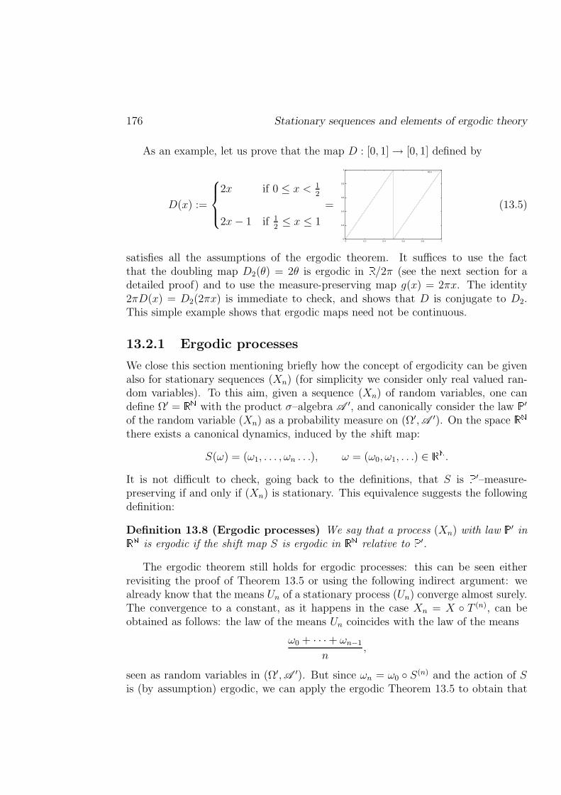
176 Stationary sequences and elements of ergodic theory
As an example, let us prove that the map D : [0, 1] → [0, 1] defined by
D(x) :=
2x if 0 ≤ x < 12
2x− 1 if 12≤ x ≤ 1
=
0
0.2
0.4
0.6
0.8
1
0 0.2 0.4 0.6 0.8 1
D(x)
(13.5)
satisfies all the assumptions of the ergodic theorem. It suffices to use the factthat the doubling map D2(θ) = 2θ is ergodic in
/2π (see the next section for a
detailed proof) and to use the measure-preserving map g(x) = 2πx. The identity2πD(x) = D2(2πx) is immediate to check, and shows that D is conjugate to D2.This simple example shows that ergodic maps need not be continuous.
13.2.1 Ergodic processes
We close this section mentioning briefly how the concept of ergodicity can be givenalso for stationary sequences (Xn) (for simplicity we consider only real valued ran-dom variables). To this aim, given a sequence (Xn) of random variables, one candefine Ω′ =
with the product σ–algebra A ′, and canonically consider the law′
of the random variable (Xn) as a probability measure on (Ω′,A ′). On the space
there exists a canonical dynamics, induced by the shift map:
S(ω) = (ω1, . . . , ωn . . .), ω = (ω0, ω1, . . .) ∈ .
It is not difficult to check, going back to the definitions, that S is′–measure-
preserving if and only if (Xn) is stationary. This equivalence suggests the followingdefinition:
Definition 13.8 (Ergodic processes) We say that a process (Xn) with law′ in
is ergodic if the shift map S is ergodic in relative to
′.
The ergodic theorem still holds for ergodic processes: this can be seen eitherrevisiting the proof of Theorem 13.5 or using the following indirect argument: wealready know that the means Un of a stationary process (Un) converge almost surely.The convergence to a constant, as it happens in the case Xn = X T (n), can beobtained as follows: the law of the means Un coincides with the law of the means
ω0 + · · ·+ ωn−1
n,
seen as random variables in (Ω′,A ′). But since ωn = ω0 S(n) and the action of Sis (by assumption) ergodic, we can apply the ergodic Theorem 13.5 to obtain that
Chapter13 177
U ′n, and therefore Un, converge in law to a constant. Since almost sure convergence
implies convergence in law we obtain that Un converge to a constant almost surely.
Some dynamical systems, when read in suitable coordinates, can be read asdynamical systems induced by a shift map. Here is a typical example: let us considermap D2 in (13.5) and the map g : 0, 1 → [0, 1] defined by
g((an)) :=∞∑
n=0
an2−n−1
(notice that g is not injective, because dyadic numbers k/2m have two binary ex-pansions). Then, D is conjugate to the shift map S in 0, 1 via g: indeed, it isnot difficult to check that x = g((an)) =
∑i ai2
−i−1 implies D(x) =∑
i ai+12−i−1,
which means precisely that g(S((an))) = D(g((an))).
13.3 Examples
In this section we present some fundamental examples of ergodic dynamical systems.
13.3.1 Arithmetic progressions on the circle
Let Ω = S1 ∼ /2π with the Borel σ–algebra and the law induced by arclength,
divided by 2π. For α ∈ S1 the map T (θ) = θ + α is easily shown to be measure-preserving and T (n)(θ) = θ + nα.
Let us prove now that if α/π /∈ then T is ergodic; we give an elementary proof,based on the fact that the group
nα + 2πm : n, m ∈ is dense in
, and another one, based on Fourier series. The first argument goes as
follows: setting u =
A, and thinking of u as a 2π-periodic function, invariance andperiodicity we get
u(θ + nα + 2πm) = u(θ) for L 1-a.e. θ,
for any n, m ∈ . Multiplying both sides by a 2π-periodic function φ we get
0 =
∫ 2π
0
u(θ + nα + 2πm) − u(θ)
nα + 2πmφ(θ) dθ =
∫ 2π
0
u(θ)φ(θ − nα− 2πm) − φ(θ)
nα + 2πmdθ
for any n, m ∈ . If φ′ exists and is bounded in (0, 2π), choosing sequences (nk)and (mk) such that nkα + 2πmk ↓ 0 we can pass to the limit as k → ∞ to obtain
∫ 2π
0
u(θ)φ′(θ) dθ = 0 ∀φ ∈ C1c (0, 2π).
178 Stationary sequences and elements of ergodic theory
Lemma 13.9 below tells us that either(A) = 0 or
(A) = 1.
The second proof goes as follows: let
u(θ) =∑
k∈
ukeikθ
be the Fourier series of u, and take the left composition with T (that preserves, bythe measure preserving property of T , the L2 convergence of the series) to obtain
u(θ) = u T (θ) =∑
k∈
ukeikαeikθ.
The uniqueness of the Fourier expansion gives that eikα = 1 for any k such thatuk 6= 0. If u is not identically equal to 0, there exists such a k, and therefore1 = eikα. As α/(2π) /∈ , this can happen only if k = 0, i.e.
A is equivalent to the
constant 1.Therefore the ergodic theorem gives
limn→∞
1
n
n−1∑
i=0
X(θ + iα) =1
2π
∫ 2π
0
X(θ) dθ
almost surely (with respect to the initial point θ) for any random variable X ∈ L1.In the previous formula we can choose in particular any bounded continuous
function X on the circle, to obtain that∑n−1
0 δθ+iα/n weakly converge to
asn→ ∞ for almost any θ. In this particular case, as the sequences θ+ iα and θ+ iαdiffer by an additive constant and the limit measure is translation invariant, thevalidity of this property for some θ implies its validity for all others.
When instead α/2π = p/q is a rational number then T is measure preserving,but not ergodic: it suffices to take a small sector S with (normalized) length lessthan 1/q and define
A :=
q−1⋃
i=0
T (i)(S),
to obtain a T -invariant set with measure q(S) ∈ (0, 1).
Notice also that, taking X(θ) = θ, we have a stationary but not independentsequence, not even pairwise independent: indeed the difference Xn−Xm is constant,therefore Xn is not independent of Xm, as seen in Exercise 10.10.
Finally, let us state and prove Lemma 13.9, that we used to show that arithmeticprogressions on the circle are ergodic.
Lemma 13.9 (De La Vallee Poussin) Let I = (a, b) be a bounded interval and
let u ∈ L1(a, b) be such that∫ b
auφ′ dt = 0 for any φ ∈ C1([a, b]) with φ(a) = φ(b).
Then there exists a constant c such that u = c L 1–almost everywhere in (a, b).
Chapter13 179
Proof. We give an elementary proof of the lemma. By a change of variableswe can assume with no loss of generality that I = (0, 1). Note that u is almosteverywhere equal to a constant in (0, 1) if and only if
∫ 1
0
uψ dt = (
∫ 1
0
u dt)(
∫ 1
0
ψ dt) (13.6)
for any continuous function ψ : [0, 1] → : indeed the above identity can be written
as ∫ 1
0
(u− (
∫ 1
0
u dt))ψ dt = 0,
and the density of continuous functions in L2(0, 1) shows that u =∫ 1
0u dtL 1-almost
everywhere in (0, 1).
Given ψ ∈ C([0, 1]), let c =∫ 1
0ψ dt, and define φ(t) :=
∫ t
0(ψ − c) ds; then
φ(0) = φ(1) = 0, so that the assumption on u gives
0 =
∫ 1
0
uφ′ dt =
∫ 1
0
u(ψ − c) dt =
∫ 1
0
uψ dt− (
∫ 1
0
u dt)(
∫ 1
0
ψ dt),
that is precisely (13.6).
13.3.2 Geometric progressions on the circle
Let m ≥ 1 be an integer. The map Dm : S1 → S1 defined by θ 7→ mθ satisfies all theassumptions of the ergodic theorem. This example shows that ergodic maps neednot be injective.
First, Dm is measure-preserving: for instance in the case m = 2 (the general caseis analogous) we see that
D−12 (A) =
1
2A ∪
(π +
1
2A
)∀A ∈ B(S1). (13.7)
Now, let us prove the ergodicity of Dm. If S ⊂ S1 is Dm-invariant, we easily seethat
∫
S1
S(θ)e−inmθ d
(θ) =
∫
S1
S(mθ)e−inmθ d
(θ) =
∫
S1
S(θ)e−inθ d
(θ)
(in the first equality we used the invariance of S, and in the second one the measure-preserving property of Dm). Repeating k times this argument we get
∫
S1
S(θ)e−inmkθ d
(θ) =
∫
S1
S(θ)e−inθ d
(θ) ∀k ∈
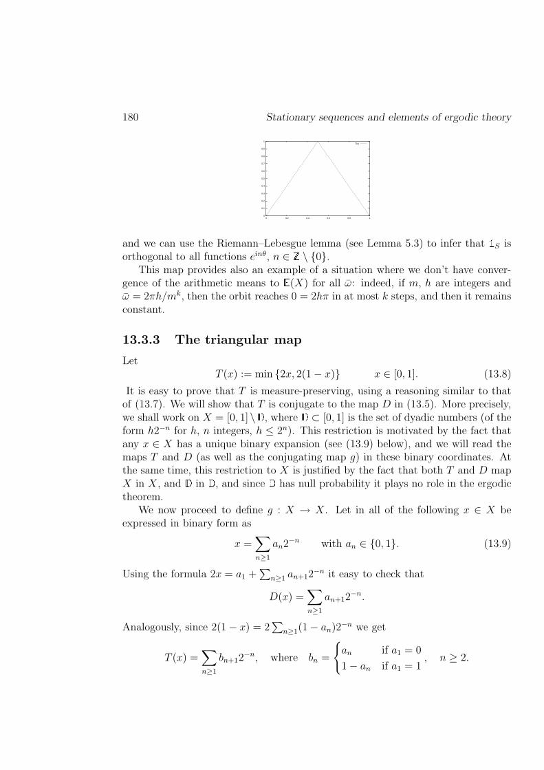
180 Stationary sequences and elements of ergodic theory
0
0.1
0.2
0.3
0.4
0.5
0.6
0.7
0.8
0.9
1
0 0.2 0.4 0.6 0.8 1
T(x)
and we can use the Riemann–Lebesgue lemma (see Lemma 5.3) to infer that
S isorthogonal to all functions einθ, n ∈ \ 0.
This map provides also an example of a situation where we don’t have conver-gence of the arithmetic means to
(X) for all ω: indeed, if m, h are integers and
ω = 2πh/mk, then the orbit reaches 0 = 2hπ in at most k steps, and then it remainsconstant.
13.3.3 The triangular map
LetT (x) := min 2x, 2(1 − x) x ∈ [0, 1]. (13.8)
It is easy to prove that T is measure-preserving, using a reasoning similar to thatof (13.7). We will show that T is conjugate to the map D in (13.5). More precisely,we shall work on X = [0, 1]\ , where
⊂ [0, 1] is the set of dyadic numbers (of theform h2−n for h, n integers, h ≤ 2n). This restriction is motivated by the fact thatany x ∈ X has a unique binary expansion (see (13.9) below), and we will read themaps T and D (as well as the conjugating map g) in these binary coordinates. Atthe same time, this restriction to X is justified by the fact that both T and D mapX in X, and
in
, and since
has null probability it plays no role in the ergodic
theorem.We now proceed to define g : X → X. Let in all of the following x ∈ X be
expressed in binary form as
x =∑
n≥1
an2−n with an ∈ 0, 1. (13.9)
Using the formula 2x = a1 +∑
n≥1 an+12−n it easy to check that
D(x) =∑
n≥1
an+12−n.
Analogously, since 2(1 − x) = 2∑
n≥1(1 − an)2−n we get
T (x) =∑
n≥1
bn+12−n, where bn =
an if a1 = 0
1 − an if a1 = 1, n ≥ 2.
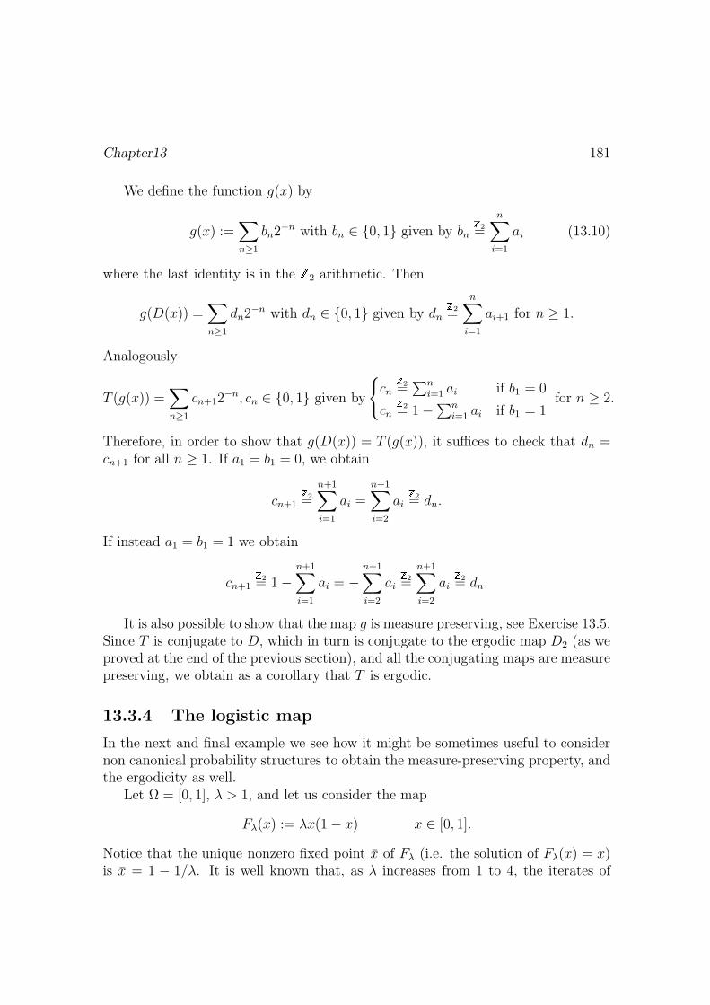
Chapter13 181
We define the function g(x) by
g(x) :=∑
n≥1
bn2−n with bn ∈ 0, 1 given by bn2=
n∑
i=1
ai (13.10)
where the last identity is in the 2 arithmetic. Then
g(D(x)) =∑
n≥1
dn2−n with dn ∈ 0, 1 given by dn
2=
n∑
i=1
ai+1 for n ≥ 1.
Analogously
T (g(x)) =∑
n≥1
cn+12−n, cn ∈ 0, 1 given by
cn
2=∑n
i=1 ai if b1 = 0
cn2= 1 −∑n
i=1 ai if b1 = 1for n ≥ 2.
Therefore, in order to show that g(D(x)) = T (g(x)), it suffices to check that dn =cn+1 for all n ≥ 1. If a1 = b1 = 0, we obtain
cn+12=
n+1∑
i=1
ai =n+1∑
i=2
ai2= dn.
If instead a1 = b1 = 1 we obtain
cn+12= 1 −
n+1∑
i=1
ai = −n+1∑
i=2
ai2=
n+1∑
i=2
ai2= dn.
It is also possible to show that the map g is measure preserving, see Exercise 13.5.Since T is conjugate to D, which in turn is conjugate to the ergodic map D2 (as weproved at the end of the previous section), and all the conjugating maps are measurepreserving, we obtain as a corollary that T is ergodic.
13.3.4 The logistic map
In the next and final example we see how it might be sometimes useful to considernon canonical probability structures to obtain the measure-preserving property, andthe ergodicity as well.
Let Ω = [0, 1], λ > 1, and let us consider the map
Fλ(x) := λx(1 − x) x ∈ [0, 1].
Notice that the unique nonzero fixed point x of Fλ (i.e. the solution of Fλ(x) = x)is x = 1 − 1/λ. It is well known that, as λ increases from 1 to 4, the iterates of
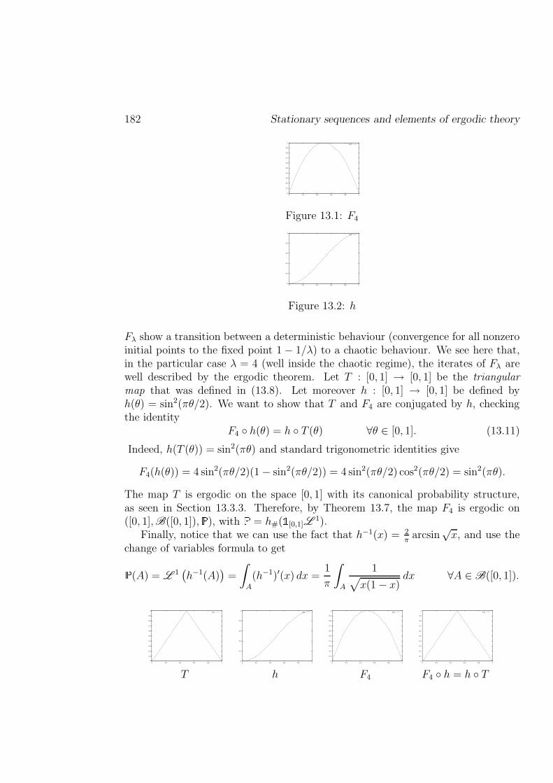
182 Stationary sequences and elements of ergodic theory
0
0.1
0.2
0.3
0.4
0.5
0.6
0.7
0.8
0.9
1
0 0.2 0.4 0.6 0.8 1
F(x)
Figure 13.1: F4
0
0.2
0.4
0.6
0.8
1
0 0.2 0.4 0.6 0.8 1
h(x)
Figure 13.2: h
Fλ show a transition between a deterministic behaviour (convergence for all nonzeroinitial points to the fixed point 1 − 1/λ) to a chaotic behaviour. We see here that,in the particular case λ = 4 (well inside the chaotic regime), the iterates of Fλ arewell described by the ergodic theorem. Let T : [0, 1] → [0, 1] be the triangularmap that was defined in (13.8). Let moreover h : [0, 1] → [0, 1] be defined byh(θ) = sin2(πθ/2). We want to show that T and F4 are conjugated by h, checkingthe identity
F4 h(θ) = h T (θ) ∀θ ∈ [0, 1]. (13.11)
Indeed, h(T (θ)) = sin2(πθ) and standard trigonometric identities give
F4(h(θ)) = 4 sin2(πθ/2)(1 − sin2(πθ/2)) = 4 sin2(πθ/2) cos2(πθ/2) = sin2(πθ).
The map T is ergodic on the space [0, 1] with its canonical probability structure,as seen in Section 13.3.3. Therefore, by Theorem 13.7, the map F4 is ergodic on([0, 1],B([0, 1]),
), with
= h#(
[0,1]L
1).Finally, notice that we can use the fact that h−1(x) = 2
πarcsin
√x, and use the
change of variables formula to get
(A) = L 1
(h−1(A)
)=
∫
A
(h−1)′(x) dx =1
π
∫
A
1√x(1 − x)
dx ∀A ∈ B([0, 1]).
0
0.1
0.2
0.3
0.4
0.5
0.6
0.7
0.8
0.9
1
0 0.2 0.4 0.6 0.8 1
T(x)
0
0.2
0.4
0.6
0.8
1
0 0.2 0.4 0.6 0.8 1
h(x)
0
0.1
0.2
0.3
0.4
0.5
0.6
0.7
0.8
0.9
1
0 0.2 0.4 0.6 0.8 1
F(x)
0
0.1
0.2
0.3
0.4
0.5
0.6
0.7
0.8
0.9
1
0 0.2 0.4 0.6 0.8 1
T(x)
T h F4 F4 h = h T
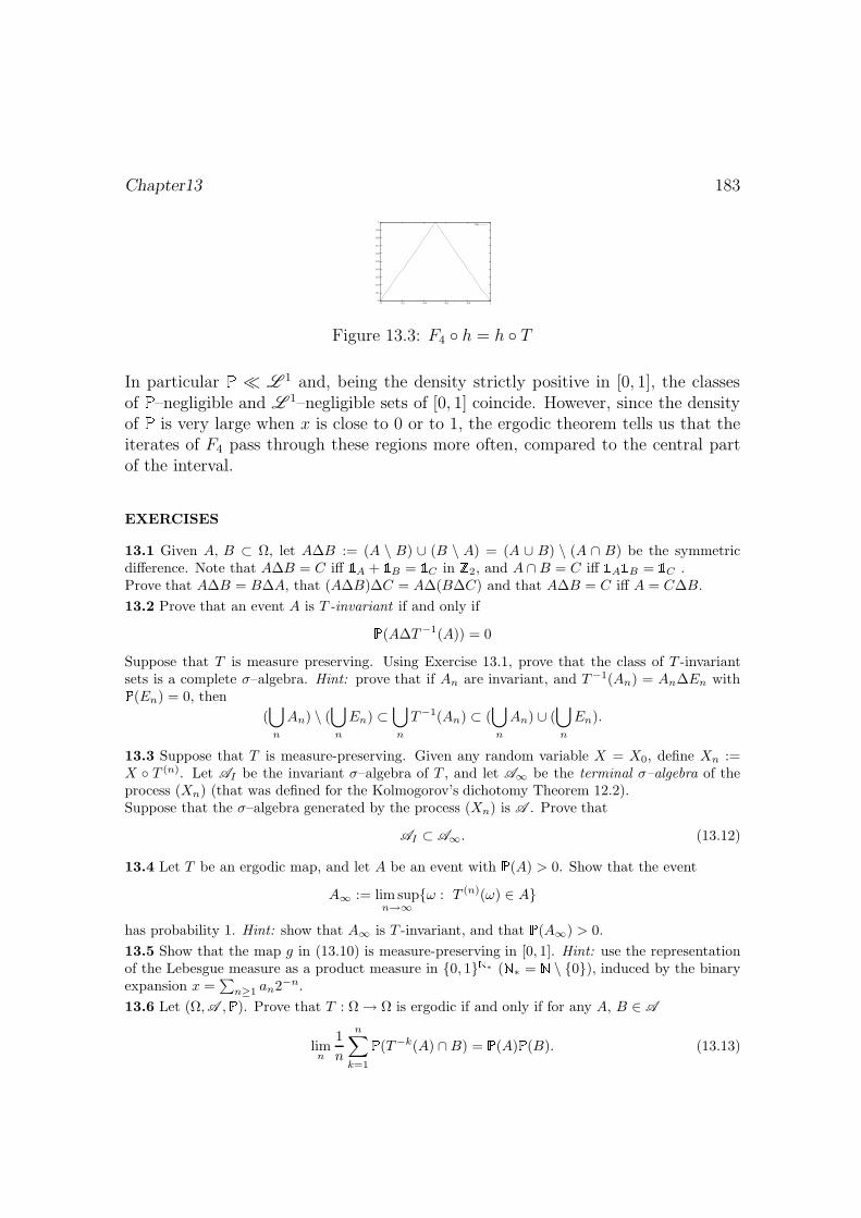
Chapter13 183
0
0.1
0.2
0.3
0.4
0.5
0.6
0.7
0.8
0.9
1
0 0.2 0.4 0.6 0.8 1
T(x)
Figure 13.3: F4 h = h T
In particular L 1 and, being the density strictly positive in [0, 1], the classes
of–negligible and L 1–negligible sets of [0, 1] coincide. However, since the density
of
is very large when x is close to 0 or to 1, the ergodic theorem tells us that theiterates of F4 pass through these regions more often, compared to the central partof the interval.
EXERCISES
13.1 Given A, B ⊂ Ω, let A∆B := (A \ B) ∪ (B \ A) = (A ∪ B) \ (A ∩ B) be the symmetricdifference. Note that A∆B = C iff A + B = C in
2, and A ∩B = C iff AB = C .
Prove that A∆B = B∆A, that (A∆B)∆C = A∆(B∆C) and that A∆B = C iff A = C∆B.
13.2 Prove that an event A is T -invariant if and only if
(A∆T−1(A)) = 0
Suppose that T is measure preserving. Using Exercise 13.1, prove that the class of T -invariantsets is a complete σ–algebra. Hint: prove that if An are invariant, and T−1(An) = An∆En with(En) = 0, then
(⋃
n
An) \ (⋃
n
En) ⊂⋃
n
T−1(An) ⊂ (⋃
n
An) ∪ (⋃
n
En).
13.3 Suppose that T is measure-preserving. Given any random variable X = X0, define Xn :=X T (n). Let AI be the invariant σ–algebra of T , and let A∞ be the terminal σ–algebra of theprocess (Xn) (that was defined for the Kolmogorov’s dichotomy Theorem 12.2).Suppose that the σ–algebra generated by the process (Xn) is A . Prove that
AI ⊂ A∞. (13.12)
13.4 Let T be an ergodic map, and let A be an event with (A) > 0. Show that the event
A∞ := lim supn→∞
ω : T (n)(ω) ∈ A
has probability 1. Hint: show that A∞ is T -invariant, and that (A∞) > 0.
13.5 Show that the map g in (13.10) is measure-preserving in [0, 1]. Hint: use the representationof the Lebesgue measure as a product measure in 0, 1∗ (∗ = \ 0), induced by the binaryexpansion x =
∑n≥1 an2−n.
13.6 Let (Ω,A , ). Prove that T : Ω → Ω is ergodic if and only if for any A, B ∈ A
limn
1
n
n∑
k=1
(T−k(A) ∩B) = (A)(B). (13.13)
184 Stationary sequences and elements of ergodic theory
Hint: Let f = A, so rewrite the above as
(T−k(A) ∩B) =
∫
B
f(T k(ω)) (dω)
Let then Xk(ω) = f(T k(ω)) by the ergodic Theorem 13.5,
limn
1
n
n−1∑
k=0
Xn = (X0)
in L1, and this means that
limn
∫
B
1
n
n−1∑
k=0
Xk(ω) (dω) =1
n
n−1∑
k=0
∫
B
Xk(ω) (dω) = (B)(X0).
Conversely, suppose that (13.13) holds; let A be T -invariant; then (T−k(A) ∩B) = (A ∩B), so(13.13) becomes (A ∩ B) = (A)(B) for all B ∈ A . In particular (A) = 2(A), that implies(A) ∈ 0, 1.13.7 Let (Ω,A , ) be a probability space and let T : Ω → Ω be a measure-preserving map. LetL2 = L2(Ω,A , ). Define U : L2 → L2 by U(X) = X T ; prove that it is linear and unitary (thatis, 〈U(X), U(Y )〉 = 〈X,Y 〉 for all X, Y ∈ L2).
13.8[Von Neumann Ergodic Theorem] Let (Ω,A , ) be a probability space and let T : Ω → Ωbe a measure preserving map. Let L2 = L2(Ω,A , ).Let AI be the invariant σ–algebra of T , so that H = L2(Ω,AI , ) is the set of square-integrable T –invariant functions. Prove that H is closed in L2 and let π : L2 → H be the orthogonal projection.Prove that, for any random variable X ∈ L2, the arithmetic means
1
n(X +X T + . . .+X T (n−1))
converge in L2 to π(X). Hint: Decompose L2 = H ⊕ K, with K the orthogonal of H, anddecompose X = X ′ + X ′′ with X ′ = π(X) ∈ H and X ′′ ∈ K. Define U : L2 → L2
by U(X) = X T ; recall the previous exercise; note that U(H) = H and prove thatU(K) ⊥ H, that means that U(K) ⊂ K. Let Zn be the linear operator
Zn(X) :=1
n(X +X T + . . .+X T (n−1)) =
1
n(X + U(X) + . . . + Un−1(X))
then U (n)(X ′) = Zn(X ′) = X ′; while Zn(X ′′) ∈ K. By Theorem 13.3, limn Zn(X) = Yin L2, and limn Zn(X ′′) = Y ′′ ∈ K; note that Y = X ′ + Y ′′. Arguing as in the Ergodictheorem 13.5, prove that Y ∈ H: then Y ′′ = 0, so limn Zn(X) = X ′ = π(X).
Chapter 14
Brownian motion
The Brownian motion is a fundamental object of Probability theory and in particularof the theory of diffusion processes. As in Analysis, where the real line
plays a
similar basic role, it can be introduced either through an axiomatic characterization,or through an explicit construction. We will follow both approaches, presenting theconstruction based on a series of Gaussian vectors. Keeping the analogy with thereal line
, many other constructions are indeed possible, see for instance [11] for
another classical one.
14.1 Discrete random walks
In this section we study a natural discrete version of the Brownian motion, therandom walk in
d on a discrete lattice hd with mesh size h > 0, with a time stepτ > 0.
To this aim, we fix a probability space (Ω,A ,) on which we can define an
independent sequence (ξk)k≥1ofd-valued random variables with
(ξk = ei) =
(ξk = −ei) =
1
2d, i = 1, . . . , d,
where e1, . . . , ed is the canonical basis ofd. Notice that
(ξk,i) = 0 and
(ξ2
k,i) = 1/d(here ξk,i is the i-th component of ξk). Then, we define random variables Sn : Ω →d ⊂ d as follows:
S0 := 0, Sn :=n∑
k=1
ξk, n ≥ 1.
We may immagine that Sn describes the position of a random walk on d after ntime steps. Denoting by Sn,i the i-th component of Sn, it is easily checked that
(Sn,i) = 0,
(Sk,iξk+1,i) = 0,
(S2
n,i) =n
d, i = 1, . . . , d. (14.1)
185
186 Brownian motion
Now, putting in the scale parameter h and the time parameter τ > 0, we can define
Xh,τ (t) := hSn when t = nτ , n ∈ .
When t/τ is not an integer we do a piecewise linear interpolation and set (here, wedenote by [x] the integer part of x ≥ 0, and by x = x− [x] the non-integer part)
Xh,τ(t) := h(1 −t
τ
)S[t/τ ] + h
t
τ
S[t/τ ]+1 = hS[t/τ ] + h
t
τ
ξ[t/τ ]+1, t ≥ 0.
It is natural to investigate the asymptotic behaviour, in the sense of probabilitytheory, of Xh,τ as h + τ → 0: this corresponds in some sense to the macroscopicbehaviour of the typical random walk. Notice first that (14.1) gives
(Xh,τ
i (t)) = 0and (
|Xh,τ(t)|2)
= h2
[t
τ
]+ h2
t
τ
2
i = 1, . . . , d. (14.2)
Therefore, in order to avoid triviality of the limit, it is natural to require that h andτ tend to 0 in such a way that h2 ∼ τ . Therefore, up to a change of scale, in thefollowing we shall assume that τ = h2.
To guess the properties that any limit X(t) of Xh,h2(t) should have, let us fix
two discrete times s = mh2, t = nh2, with m < n, and let us notice that
Xh,h2
(t) −Xh,h2
(s) = hn∑
k=m+1
ξk.
Notice that each component of the right hand side is a centered random variable withvariance σ2 = h2(n−m)/d. The same argument, based on the Levy theorem, usedfor the proof of the central limit theorem shows that this sum, when rescaled by thevariance, asymptotically displays a Gaussian distribution N (0, 1); as a consequence,
Xh,h2
i (t)−Xh,h2
i (s) converges in law to N (0, σ2) = N (0, (t−s)/d) for all i = 1, . . . , d.Let us fix now finitely many discrete times tj = mjh
2, with m1 < · · · < mn, andnotice that
Xh,h2
(t1), Xh,h2
(t2) −Xh,h2
(t1), . . . , Xh,h2
(tn) −Xh,h2
(tn−1)
are independent. Indeed, these differences are given by
h
m1∑
k=1
ξk, h
m2∑
k=m1+1
ξk, . . . , h
mn∑
k=mn−1+1
ξk,
and the independence of the sequence (ξk) can be applied.Therefore, it is natural to conjecture that any “limit” X(t) (in a sense to be
specified) of Xh,h2(t) as h→ 0 should satisfy:
Chapter 14 187
(i) X(0) = 0 almost surely;
(ii) the law of Xi(t) − Xi(s) is N (0, (t − s)/d) whenever 0 ≤ s < t and i ∈1, . . . , d;
(iii) For any choice of times 0 = t0 ≤ t1 ≤ · · · ≤ tn, the variables
X(tj) −X(tj−1) : j ∈ 1, . . . , n
are independent.
Property (iii) is the stronger one, and it is usually recalled by saying that the stochas-tic process X(t) has independent increments.
Indeed, it is possible to show that this guess is correct: namely, a limit stochasticprocess X(t) exists, in the sense that for any choice of times 0 = t0 < t1 < · · · < tnthe
nd-valued random variablesXh,h2
i (tj) −Xh,h2
i (tj−1) : i ∈ 1, . . . , d, j ∈ 1, . . . , n
converge in law, as h→ 0, to
Xi(tj) −Xi(tj−1) : i ∈ 1, . . . , d, j ∈ 1, . . . , n
.
Furthermore, X satisfies (i), (ii) and (iii). Actually (ii) holds in a stronger form,because also the components Xi(t)−Xi(s) are independent (see also Exercise 14.1).In addition, the continuity and even some mild regularity property of the randomtrajectories is preserved in the limit.
However, in this more elementary textbook we will just prove, in the next sec-tions, the existence of a stochastic process fulfilling (i), (ii) and (iii) above, and provesome of its regularity properties. Furthermore, we will prove that the law of X isunique, the so-called Wiener measure in C([0,∞);
d).
14.2 Some properties of Gaussian random vari-
ables
In this section we extend from the real to thed-valued case the theory of Gaussian
random variables. Recall that in the real case the Gaussian law N (0, σ2), withσ > 0, has (2πσ2)−1/2 exp(−x2/2σ2) as density with respect to L 1. It is alsouseful to extend “by continuity” the notation N (0, σ2) to the case σ = 0, settingN (0, 0) = δ0.
188 Brownian motion
For laws ind, we start by defining N (0, Id), where Id is the identity d × d
matrix, as the absolutely continuous measure ind with density
1
(2π)d/2exp
(−|x|2
2
)
with respect to L d. Since |x|2 = |x1|2 + · · · + |xd|2, N (0, Id) is nothing but theproduct of d copies of N (0, 1).
Let now Q be a symmetric and positive definite matrix; we define N (0, Q) asthe absolutely continuous measure in
d with density
1√(2π)ddetQ
exp
(−〈Q−1x, x〉
2
).
More generally, the definition above can be given for any nonnegative and symmetricbilinear form Q in a d-dimensional Hilbert space H : given an orthonormal systemε1, . . . , εd, we consider the symmetrix matrix Q representing Q with respect tothis system (i.e. Qij = 〈Qεi, εj〉 and the Gaussian measure N (0, Q) in
d; then,N (0, Q) is defined as the law of the map x 7→∑
i xiεi. It is not hard to show (usingthe invariance of determinant and Lebesgue measure under rotations in
d) thatthis definition is independent of the choice of coordinates.
In the case when Q is symmetric and nonnegative definite we still need to defineN (0, Q): to do this, we canonically split
d = H ⊕ KerQ,
where Q is positive definite on H , and denote by Q : H × H → the positive
bilinear form induced by Q, by restriction. Then, we define
N (0, Q) := N (0, Q) × δ0, (14.3)
where the first factor N (0, Q) is the Gaussian in H induced by Q and the secondfactor is the Dirac mass at the origin of Ker Q. Gaussian measures N (0, Q) arecalled non-degenerate if Q is positive definite, and degenerate otherwise.
Definition 14.1 (Gaussian vector) Let X be ad-valued random variable. We
say that X is a Gaussian vector if its law is N (0, Q) for some symmetric andnonnegative definite matrix Q.
Let σ21, . . . , σ
2d be the eigenvalues of Q and let ε1, . . . , εd be the correspond-
ing orthonormal basis of eigenvectors; if we denote by xi = 〈x, εi〉 the coordinates
Chapter 14 189
induced by this basis, and assume that σi > 0, we can write the density of N (0, Q)as a product, namely
N (0, Q) =
d∏
i=1
1√2πσ2
i
exp
(−|xi|2
2σ2i
)L d. (14.4)
As a consequence, in this system of coordinates x1, . . . , xd are independent, andxi has law N (0, σ2
i ). In the case when some of the σi vanish we still have a productstructure with Dirac masses on some factors, see (14.3).
This fact suggests a simple and useful criterion for the verification of the inde-pendence of the components of a Gaussian vector.
Theorem 14.2 (Independence criterion of Gaussian vectors) Let
X = (X1, . . . , Xd)
be a Gaussian vector with law N (0, Q). Then
〈Qh, k〉 =
(〈X, h〉〈X, k〉) =
d∑
i, j=1
hikj
(XiXj) ∀h, k ∈ d. (14.5)
In particular Q is a diagonal matrix, and therefore (X1, . . . , Xd) are independent, ifand only if
(XiXj) = 0 for i 6= j.
Proof. Since the law of X is N (0, Q), we have to show that
〈Qh, k〉 =
∫
d
〈x, h〉〈x, k〉 dN (0, Q) ∀h, k ∈ d. (14.6)
Next, we check (14.6) in the basis ε1, . . . , εd where Q is diagonal. We denote, asabove, by xi the coordinates of x in this basis and by σ2
i the eigenvalues of Q anduse (14.4) to obtain
∫
d
〈x, h〉 〈x, h〉 dN (0, Q)(x) =d∑
i, j=1
〈h, εi〉 〈k, εj〉∫
d
xi xj dN (0, Q)(x)
=d∑
i=1
〈h, εi〉 〈k, εi〉∫
d
(xi)2 dN (0, Q)(x)
+∑
i6=j
〈h, εi〉 〈k, εj〉(∫
d
xi dN (0, Q)(x)
) (∫
d
xi dN (0, Q)(x)
)
=
d∑
i=1
〈h, εi〉 〈k, εi〉 σ2i = 〈Qh, k〉.
190 Brownian motion
The matrix Q is also called covariance matrix of the Gaussian vector X, thename being justified by (14.5). In particular 〈Qh, h〉 coincides with
(|〈X, h〉|2),
and tells us how much X is “spread” in the direction h.Next, we consider sums of Gaussian vectors.
Proposition 14.3 (Sum of independent Gaussian vectors) Let X, X ′ be in-dependent d-dimensional Gaussian vectors, respectively with laws N (0, Q) and N (0, Q′).Then X + Y is still a Gaussian vector, with law N (0, Q+Q′).
Proof. By the independence of X and X ′, (X,X ′) is a 2d-dimensional Gaussianvector with law N (0, Q), where
〈Q(x, y), (x, y)〉 = 〈Qx, x〉 + 〈Q′y, y〉.
By Exercise 14.2 (X + X ′, X − X ′) is still a 2d-dimensional Gaussian vector, andX + X ′ is a d-dimensional Gaussian vector. Denoting by R the covariance matrixof X +X ′, from (14.5) and the independence of 〈X, h〉 and 〈X ′, k〉 we get
〈Rh, k〉 =
(〈X +X ′, h〉〈X +X ′, k〉)
=
(〈X, h〉〈X, k〉) +
(〈X ′, h〉〈X ′, k〉)
= 〈Qh, k〉 + 〈Q′h, k〉
for all h, k ∈ d. Therefore R = Q+Q′.
Theorem 14.4 (Series of independent Gaussian vectors) Let
(Xn) = ((Xn,1, . . . , Xn,d))
be an independent sequence of d-dimensional Gaussian vectors, with law N (0, Qn).Then, if the series
∑nQn is convergent, the series
∑nXn is convergent almost
surely and in L2, and the sum S is still a Gaussian vector, with law N (0,∑
nQn).
Proof. Taking into account the independence of Xn and (14.3), we have
(|
m∑
i=n
Xi,j|2) =
m∑
i=n
(|Xi,j|2) =
m∑
i=n
〈Qiej , ej〉, (14.7)
for m ≥ n ≥ 0, j = 1, . . . , d. Therefore, for any j, the partial sums∑n
0 Xi,j areCauchy in L2(Ω,A ,
) and therefore converge in L2(Ω,A ,
).
The almost sure convergence of the series∑
nXn follows by the same argumentused in the proof of part (a) of the law of large numbers, see Theorem 12.4 (one first
Chapter 14 191
shows that the partial sums∑n2
0 Xi is converging almost surely, and then that thefull sequence converges).
Finally, let us check that S is Gaussian. We already know from Proposition 14.3that
∑n0 Xi are Gaussian, and their law is N (0,
∑n0 Qi), so that
(f(
n∑
i=0
Xi)) =
∫
d
f(x) dN (0,
n∑
i=0
Qi) ∀f ∈ Cb(d).
Passing to the limit as n→ ∞, the dominated convergence theorem for the left-handside and Exercise 14.3 for the right-hand side give
(f(S)) =
∫
d
f(x) dN (0,
∞∑
i=0
Qi) ∀f ∈ Cb(d).
Therefore the law of S is N (0,∑∞
0 Qi).
14.3 d-dimensional Brownian motion
Motivated by the discrete random walk, we give the following definition of randomwalk in a space-time continuous setting.
Recall first that a family B(t)t≥0 ofd-valued random variables is a continuous
stochastic process if
t 7→ B(t)(ω) is continuous in [0,∞)
almost surely. It is also useful to consider a continuous stochastic process as a mapω 7→ B(·)(ω), i.e. as a random map with values (almost surely) in the space ofcontinuous maps in
d.
Definition 14.5 (d-dimensional Brownian motion) A d-dimensional Brownianmotion B = B(t)t≥0 is a continuous
d-valued stochastic process such that
(i) B(0) = 0 almost surely;
(ii) if 0 ≤ s < t, B(t) −B(s) is a Gaussian vector with law N (0, (t− s)Id);
(iii) if 0 = t0 ≤ t1 < · · · < tn, the nd-valued random variables
B(tj) − B(tj−1) 1 ≤ j ≤ n
are independent.
192 Brownian motion
Notice that condition (ii) is stronger than the corresponding one stated in Sec-tion 14.1, as we require also the independence of the components of B(t) − B(s).
We build a Brownian motion first in the scalar case d = 1, and then in thevectorial case. We consider an underlying probability space (Ω,A ,
) on which
an independent sequence (αk) of random variables with law N (0, 1) exists; theseprobability spaces certainly exist, see Section 10.2.
Let H = L2(0,∞) (we denote by 〈·, ·〉 the scalar product in H and by ‖ · ‖ thenorm in H) and let ekk≥1 be a complete orthonormal system in H . We recall thatfor any f ∈ H the Fourier series
f =
∞∑
k=1
fkek, with fk := 〈f, ek〉 =
∫ ∞
0
f(ξ)ek(ξ) dξ,
is convergent on H . Moreover, the Parseval equality holds
∫ ∞
0
f(ξ)g(ξ) dξ =∞∑
k=1
fkgk, f, g ∈ H. (14.8)
We define B(t) : Ω → by
B(t)(ω) =
∞∑
k=1
αk(ω)
∫ t
0
ek(ξ) dξ =
∞∑
k=1
αk(ω)〈[0,t], ek〉. (14.9)
For any t ≥ 0, B(t) is a series of independent centered Gaussian random variables.The corresponding series of the variances is given by, taking into account the Parsevalidentity (14.8),
∞∑
k=1
(∫ t
0
ek(ξ)dξ
)2
=∞∑
k=1
〈[0,t], ek〉2 =
∫ ∞
0
[0,t](s) ds = t. (14.10)
Therefore the series (14.9) is convergent almost surely and in L2(Ω,A ,), and
defines a Gaussian random variable with variance t, by Theorem 14.4.
Theorem 14.6 The stochastic process B defined in (14.9) is a Brownian motion.
Proof. As (i) is obvious, we can check (ii). For t > s ≥ 0 we have, arguing as wedid for B(t), that B(t) − B(s) is Gaussian with law N (0, t− s). In a similar way,using Theorem 14.4 one can see that, given 0 < t1 < · · · < tn, the random variablewith values in
n, (B(t1), . . . , B(tn)) is Gaussian. Indeed, all vectors
αk
(〈[0,t1], ek〉, 〈
[0,t2], ek〉, . . . , 〈
[0,tn], ek〉
)
Chapter 14 193
are degenerate Gaussian, with law N (0, Qk), where 〈Qkx, x〉 = |〈vk, x〉|2, and
vk :=(〈[0,t1], ek〉, 〈
[0,t2], ek〉, . . . , 〈
[0,tn], ek〉
)
Since, by the Parseval identity,∑
k |vk|2 <∞ we know that∑
k Qk is convergent.Let us check (iii). Let 0 = t0 < t1 < · · · < tn. To prove that the random
variables B(t1), B(t2)−B(t1), . . . , B(tn)−B(tn−1) are independent it is enough toshow, by Theorem 14.2, that their covariance operator (namely the expectation ofproducts of different components) is diagonal. In fact, if i 6= j we have, using againthe independence of αk and the Parseval identity, that
([B(ti) − B(ti−1)][B(tj) −B(tj−1)]) =
( ∞∑
k,l=1
αkαl〈
[ti−1,ti], ek〉〈
[tj−1,tj ], el〉)
=
( ∞∑
k=1
α2k〈
[ti−1,ti], ek〉〈
[tj−1,tj ], ek〉)
=
∫ ∞
0
[ti−1,ti](ξ)
[tj−1,tj ](ξ) dξ = 0.
So, (iii) is proved. It remains to prove the continuity of B(t). For this we shall usethe so-called factorization method. It is based on the following elementary identity
∫ t
s
(t− σ)α−1(σ − s)−α dσ = K(α) <∞, s < t, (14.11)
where α ∈ (0, 1) andK depends only on α. To check (14.11) it is enough to transformthe integral in (14.11), setting σ = r(t− s) + s. We find
K(α) =
∫ 1
0
(1 − r)α−1r−α dr <∞.
Identity (14.11) can be written as
[0,t](s) =
1
K(α)
∫ t
0
(t− σ)α−1[0,σ](s)(σ − s)−αdσ, s, t ≥ 0.
We can also write equivalently
[0,t](s) =
1
K(α)
∫ t
0
(t− σ)α−1gσ(s) dσ, (14.12)
194 Brownian motion
where gσ(s) =
[0,σ](s)(σ−s)−α. From now on we take α < 1/2, so that gσ ∈ H and
‖gσ‖2 =σ1−2α
1 − 2α. (14.13)
In view of (14.12) we can write
B(t) =1
K(α)
∫ t
0
(t− σ)α−1Y (σ) dσ, (14.14)
where Yσ are the random variables defined by
Y (σ) =
∞∑
k=1
αk〈gσ, ek〉. (14.15)
By (14.13) and Theorem 14.4 again we infer that Yσ is a centered Gaussian variablewith law N (0, σ1−2α/(1 − 2α)).
Now it is enough to prove that, at least for some m > 1/(2α), Y ∈ L2m(0, T )almost surely for any T > 0; this implies that B is continuous by the elementaryLemma 14.7 below.
Fix any m > 0 and T > 0. To prove that
∫ T
0
|Y (σ)|2m dσ <∞
almost surely, it is enough to show that its expectation is finite; Fubini’s theoremgives [∫ T
0
|Y (σ)|2m dσ
]=
∫ T
0
[|Y (σ)|2m
]dσ =
∫ T
0
∫
|x|2m dN (0,
σ1−2α
1 − 2α)(x) dσ
=
∫ T
0
σm(1−2α)
(1 − 2α)m
∫
|x|2m dN (0, 1)(x) dσ <∞.
This completes the construction of a 1-dimensional Brownian motion. In thegeneral case one can repeat the construction above, where now αk = (αk,1, . . . , αk,d)are
d-valued, their components αk,i have law N (0, 1), and the family
F := αk,i : k ≥ 1, 1 ≤ i ≤ d
is independent. Or, given a 1-dimensional Brownian motion B on (Ω,A ,), we can
proceed as follows: we consider d copies (Ωi,Ai,
i) of (Ω,A ,) and their product
×d
1 Ωi, endowed with the product σ–algebra and the product measure. Then, fort ≥ 0 we set
B(t)(ω) = (B(t)(ω1), . . . , B(t)(ωd)) .
Chapter 14 195
It is immediate to check thatB is continuous and that condition (ii) of Definition 14.5is fulfilled. Condition (iii) can also be easily verified, taking into account that (ωi)are independent, and that independence is stable under composition.
Lemma 14.7 Let m > 1, α ∈ ( 12m, 1), T > 0 and f ∈ L2m(0, T ). Set
F (t) :=
∫ t
0
(t− σ)α−1f(σ) dσ t ∈ [0, T ].
Then F ∈ C([0, T ]).
Proof. Let us set for ε ∈ (0, 1)
Fε(t) :=
∫ t(1−ε)
0
(t− σ)α−1f(σ) dσ, t ∈ [0, T ].
Then Fε is obviously continuous on [0, T ]. Now, notice that 2mα− 1 > 0, therefore2m(α− 1)/(2m− 1) > −1; we can apply Holder’s inequality to get
|F (t) − Fε(t)| ≤(∫ t
t(1−ε)
(t− σ)(α− 1) 2m
2m−1 dσ
)2m−12m
‖f‖L2m(0,T )
=
(2m− 1
2mα− 1
) 2m−12m
(εt)2mα−1
2m ‖f‖L2m(0,T ).
Thus limε Fε(t) = F (t) uniformly on [0, T ] as ε→ 0, and F is continuous as required.
Let us consider the set E = C([0,∞);d) of all
d-valued continuous functionson [0,+∞). It is a complete linear metric space with the distance
d(f, g) :=
∞∑
k=1
2−ksupt∈[0,k] |f(t) − g(t)|
1 + supt∈[0,k] |f(t) − g(t)| , f, g ∈ E,
that induces the uniform convergence on bounded subsets of [0,∞).Since the Brownian motion B = (B(t)) is almost surely continuous, we may
modify it (without affecting its probabilistic properties) in a–negligible set in such
a way that B(·)(ω) is continuous in [0,∞) for all ω ∈ Ω. Therefore, as we alreadysaid, B can be considered as a random variable in Ω with values on C([0,∞);
d),just considering the map ω 7→ B(·)(ω): indeed, it is not hard to show that this mapis (A ,B(E))–measurable (see Exercise 14.8). As a consequence we can consider thelaw of this random variable.
196 Brownian motion
Definition 14.8 (Wiener measure) The Wiener measure in C([0,∞);d) is
the image of
under the map ω 7→ B(·)(ω), where B is any d-dimensional Brownianmotion. It is a probability measure in C([0,∞);
d) concentrated on maps equal to0 at t = 0.
While d-dimensional Brownian motions are not unique, as the stochastic processB(t) can be built on many and quite different probability spaces, it turns out that is unique, and it does not depend on B (so, the definition above is well posed).To see how this measure can be characterized, let us denote by γ the typical elementof C([0,∞);
d) and let us consider the so-called evaluation maps
et : C([0,∞);d) → d, where et(γ) := γ(t), t ≥ 0.
Then the following result holds.
Theorem 14.9 The Wiener measure is the unique probability measure in thespace C([0,∞);
d) such that the stochastic process (et) defined on C([0,∞);d) is
a d-dimensional Brownian motion.
Proof. Existence follows by the representation of as I#, where I : Ω →
C([0,+∞);d) is defined by I(ω) = B(·)(ω), as in Definition 14.8. As et I = B(t),
the random variables et on the space C([0,+∞);d) coincide with the random vari-
ables B(t) on Ω, therefore the stochastic process (et) is a d-dimensional Brownianmotion.
In order to prove uniqueness we consider the class of bounded continuous cylin-drical functions in E = C([0,∞);
d), namely the bounded continuous functionsf on C([0,∞);
d) that depend only on finitely many evaluation maps (precisely:there exist t1, . . . , tn such that γ(ti) = γ(ti), 1 ≤ i ≤ n, implies f(γ) = f(γ)). Wewill prove that:
(a) the σ–algebra generated by cylindrical functions coincides with the Borel σ–algebra;
(b) if and ′ are Brownian motions, then∫
Ef d =
∫Ef d ′ for any continuous
and bounded cylindrical function f .
These two facts obviously imply that = ′.
In order to show (a) we prove that any f ∈ Cb(E) is the pointwise limit ofcontinuous and bounded cylindrical functions. To this aim, it suffices to build con-tinuous “finite dimensional projections” πn : E → E, with the property that πn(γ)depends only on finitely many evaluation maps et(γ), and πn(γ) → γ as n→ ∞ forall γ ∈ E. Then, one defines fn = f πn and obtains that fn → f pointwise (by the
Chapter 14 197
continuity of f) and fn are cylindrical. The maps πn can be defined as piecewiselinear interpolations as follows:
πn(γ)(t) :=
γ(n) if t ≥ n
(1 + k − nt)γ( kn) + (nt− k)γ(k+1
n) if t ∈ [ k
n, k+1
n), 0 ≤ k ≤ n2.
It is easy to check that πn(γ) depends only on the values of γ at the points k/n,0 ≤ k ≤ n2. Moreover, as any γ ∈ E is uniformly continuous in [0, T ] for all T > 0,it is immediate to show that πn(γ) → γ locally uniformly in [0,∞) (and then in thedistance of E) as n→ ∞.
In order to show (b), we have to check that
∫
E
f(et1 , . . . , etn) d =
∫
E
f(et1 , . . . , etn) d ′
for any integer n ≥ 1, t1 < · · · < tn and any bounded continuous function f :(d)n →
. Now, setting
g(z1, . . . , zn) := f(z1, z1 + z2, z1 + z2 + z3, . . . ,
n∑
k=1
zk)
we have
f(x1, . . . , xn) = g(x1, x2 − x1, . . . , xn − xn−1),
hence it suffices to show that
∫
E
g(et1 , et2 − et1 , . . . , etn − etn−1) d =
∫
E
g(et1 , . . . , etn − etn−1) d ′.
But these integrals are uniquely determined by conditions (ii) and (iii): they areequal to
∫
(d)n
g dN (0, t1Id) × N (0, (t2 − t1)Id) × · · · × N (0, (tn − tn−1)Id).
The d-dimensional Brownian motion induced by the evaluation maps et is some-how canonical, due to the natural choice of the underlying probability space, and itis called standard Brownian motion.
198 Brownian motion
14.4 Total variation of the Brownian motion
We are given a d-dimensional Brownian motion B in a probability space (Ω,A ,).
We are going to prove that, for any T > 0, B(·)(ω) has not bounded variation in[0, T ] for
–almost all ω ∈ Ω.
The variation VTf of a function f : [0, T ] → d is defined by
VT (f) := supσ∈Σ
n∑
k=1
|f(tk) − f(tk−1)|,
where Σ is the set of all decompositions
σ = 0 = t0 < t1 < · · · < tn = T
of the interval [0, T ].The set Σ is endowed with the usual partial ordering
σ1 ≤ σ2 if |σ1| ≤ |σ2|,
where, for any σ ∈ Σ, we have
|σ| := maxk=1,...,n
(tk − tk−1).
If VT (f) < ∞ we say that f has bounded variation in [0, T ]. In the case whenf is injective, thinking of f as the parameterization of a curve Γ = f(t)t∈[0,T ],VT (f) corresponds to the supremum of the lengths of the polygonals inscribed in Γ,and indeed coincides with the length of Γ if f is sufficiently regular, say of class C1.So, we are going to show that the typical trajectory of the Brownian motion has aninfinite length on any time interval [0, T ].
Remark 14.10 Assume that f ∈ C([0, T ];d) and define the quadratic variation
V 2T (f) of f by
V 2T (f) := lim sup
|σ|→0
n∑
k=1
|f(tk) − f(tk−1)|2.
Then V 2T (f) > 0 implies VT (f) = ∞. In fact, assume by contradiction that VT (f) is
finite. Then we haven∑
k=1
|f(tk) − f(tk−1)|2 ≤ supk=1,2,...,n
|f(tk) − f(tk−1)| VT (f).
Since, by the continuity of f ,
supk=1,2,...,n
|f(tk) − f(tk−1)| → 0 as |σ| → 0,
Chapter 14 199
we have
lim|σ|→0
n∑
k=1
|f(tk) − f(tk−1)|2 = 0,
a contradiction.
Let us compute the quadratic variation of B.
Proposition 14.11 For any T > 0 we have
lim|σ|→0
n∑
k=1
|B(tk) − B(tk−1)|2 = T in L2(Ω,A ,). (14.16)
In particular, almost surely B(t) has not bounded variation in [0, T ].
Proof. Let σ = 0 = t0 < t1 < ... < tn = T ∈ Σ and set
Jσ =
n∑
k=1
|B(tk) − B(tk−1)|2.
Then we have (|Jσ − T |2) =
(J2
σ) − 2T
(Jσ) + T 2. (14.17)
But (Jσ) =
n∑
k=1
(|B(tk) −B(tk−1)|2) =
n∑
k=1
(tk − tk−1) = T, (14.18)
since B(tk) − B(tk−1) is a Gaussian random variable with law N (0, tk − tk−1).Moreover
(|Jσ|2) =
∣∣∣∣∣
n∑
k=1
|B(tk) − B(tk−1)|2∣∣∣∣∣
2 =
( n∑
k=1
|B(tk) − B(tk−1)|4)
+2∑
h<k
(|B(th) − B(th−1)|2|B(tk) −B(tk−1)|2
).
But, using the identity (2π)−1/2∫x4e−x2/2 dx = 3 (that can be proved by integrating
by parts the product x3 ddxe−x2/2, using the fact that the variance of the N (0, 1) is
1) we have( n∑
k=1
|B(tk) − B(tk−1)|4)
=
n∑
k=1
1√2π(tk − tk−1)2
∫
ξ4e
− ξ2
2(tk−tk−1)dξ
= 3
n∑
k=1
(tk − tk−1)2,
(14.19)
200 Brownian motion
and, since B(th) −B(th−1) and B(tk) −B(tk−1) are independent,
∑
h<k
(|B(th) − B(th−1)|2|B(tk) −B(tk−1)|2
)=∑
h<k
(th − th−1)(tk − tk−1). (14.20)
Therefore(|Jσ|2) = 3
n∑
k=1
(tk − tk−1)2 + 2
∑
h<k
(th − th−1)(tk − tk−1)
= 2
n∑
k=1
(tk − tk−1)2 +
(n∑
k=1
(tk − tk−1)
)2
= 2n∑
k=1
(tk − tk−1)2 + T 2.
(14.21)
Substituting (14.18) and (14.21) on (14.17), yields
(|Jσ − T |2) = 2
n∑
k=1
(tk − tk−1)2 ≤ 2|σ|T → 0 as σ → 0.
Now, let us prove the last statement. Since lim|σ|→0 Jσ = T in L2(Ω,A ,), there
exist a sequence (σn) ⊂ Σ(0, T ) and a set A ∈ A such that |σn| → 0,(A) = 1
and Jσn(ω) → T for all ω ∈ A. Consequently V 2
T (B(·)ω) > 0 for all ω ∈ A andRemark 14.10 gives that VT (B(·)(ω)) = ∞ for all ω ∈ A.
EXERCISES
14.1 Compute (Sn,iSn,j) and use the result to show that (Xh,h2
i (t)Xh,h2
j (t)) is infinitesimal ash→ 0 when i 6= j.
14.2 Let X be a d-dimensional Gaussian vector. Show that
(a) T (X) is a Gaussian vector for all orthogonal maps T : d → d;
(b) (X1, . . . , Xm) is a m-dimensional Gaussian vector for all m ∈ 1, . . . , d.
14.3 Let Qi be symmetric nonnegative definite d× d matrices, converging to Q (entry by entry).Show that Q is symmetric and nonnegative definite, and that
limi→∞
∫
d
f(x) dN (0, Qi) =
∫
d
f(x) dN (0, Q) ∀f ∈ Cb(d).
Hint: Consider separately the case when Q is positive definite (in this case one can use the explicitexpressions of the density of N (0, Q) with respect to Lebesgue measure, the dominated convergencetheorem), and the case when Q is identically 0. Finally the general case can be achieved with (14.3).
Chapter 14 201
14.4? ? Let B be a d-dimensional Brownian motion and T > 0. Prove that B(·)(ω) is Holdercontinuous in [0, T ] with any exponent β < 1/2 for –almost all ω ∈ Ω. Hint: choose α ∈ (β, 1/2)and m such that α− 1/(2m) = β. Then prove that Lemma 14.7 can be improved by saying thatF ∈ C0,α−1/(2m)([0, T ]).
14.5 Let B be a d-dimensional Brownian motion and T > 0. Prove that B(·)(ω) is not Holdercontinuous in [0, T ] with exponent β > 1/2 for –almost all ω ∈ Ω. Hint: use the fact that almostsurely the quadratic variation of B(t) is strictly positive.
14.6 Let B(t) be a d-dimensional Brownian motion and λ > 0. Show that Bλ(t) = 1√λB(λt) is
still a d-dimensional Brownian motion.
14.7 Let B(t) be a d-dimensional Brownian motion. Show that
C(t) :=
1√tB(t2) if t > 0;
0 if t = 0C(t) :=
tB(1
t ) if t > 0;
0 if t = 0
are still d-dimensional Brownian motions.
14.8 Let B(t) be a d-dimensional Brownian motion, and assume that B(·)(ω) is continuous for allω ∈ Ω. Show that the map ω 7→ B(·)(ω) is measurable, with respect to the σ–algebra A and theBorel σ–algebra of C([0,∞); d).

202 Brownian motion
Bibliography
[1] L.Carleson: On the convergence and growth of Fourier series. Acta Math.,116 (1966), 135–157.
[2] Il caos – le leggi del disordine, a cura di Giulio Casati, Le Scienze Editore, Milano,1991.
[3] R.L.Devaney: An introduction to chaotic dynamical systems, Addison–Wesley,New York, 1987.
[4] H.Federer: Geometric Measure Theory. Springer, 1969.
[5] G.B.Folland: A course in abstract harmonic analysis. Studies in AdvancedMathematics, CRC Press, 1995.
[6] E.Giusti: Analisi II. Bollati Boringhieri, 1989.
[7] J.Jacod & P.Protter: Probability essentials. Springer, 2000.
[8] G.Letta: Probabilita elementare. Zanichelli, 1993.
[9] N.Pintacuda: Probabilita. Decibel, 1994.
[10] W.Rudin: Real and complex analysis. Mc Graw–Hill, 1987.
[11] D.W. Stroock, S.R.S. Varadhan (1997): Multidimensional diffusion pro-cesses. Springer Verlag, second ed.
[12] S.Wagon: The Banach-Tarski paradox. Cambridge University Press, 1985.
[13] K.Yosida: Functional Analysis. Springer, 1980.