Contributions to the Theory of Unequal Probability Sampling

Anders Lundquist

Doctoral Dissertation Department of Mathematics and Mathematical Statistics Umeå University SE-90187 Umeå Sweden

Copyright © Anders Lundquist ISBN:978-91-7264-760-2 Printed by: Print & Media Umeå 2009

Contents

List of papers iv

Abstract v

Preface vii

1 Introduction 1

2 Random sampling and inference 22.1 Definitions and notation . . . . . . . . . . . . . . . . . . . . . . . . . 22.2 Inference in survey sampling . . . . . . . . . . . . . . . . . . . . . . . 32.3 Further considerations regarding inference . . . . . . . . . . . . . . . 5

3 Some πps designs and related results 63.1 The CP design . . . . . . . . . . . . . . . . . . . . . . . . . . . . . . 73.2 The Sampford design . . . . . . . . . . . . . . . . . . . . . . . . . . . 83.3 The Pareto design . . . . . . . . . . . . . . . . . . . . . . . . . . . . . 83.4 Choosing pk:s for the CP and Pareto designs . . . . . . . . . . . . . . 8

3.4.1 Analytic results - the CP design . . . . . . . . . . . . . . . . . 93.4.2 Analytic results - the Pareto design . . . . . . . . . . . . . . . 103.4.3 A little about iterative procedures . . . . . . . . . . . . . . . . 11

3.5 Sampling with desired second-order inclusion probabilities . . . . . . 123.6 On measuring probabilistic distances . . . . . . . . . . . . . . . . . . 123.7 On balanced sampling with maximum entropy . . . . . . . . . . . . . 13

4 Summary of the papers 154.1 Paper I. Pareto sampling versus Sampford and conditional Poisson

sampling . . . . . . . . . . . . . . . . . . . . . . . . . . . . . . . . . . 154.2 Paper II. On sampling with desired inclusion probabilities of first and

second order . . . . . . . . . . . . . . . . . . . . . . . . . . . . . . . . 164.3 Paper III. On the distance between some πps sampling designs . . . . 164.4 Paper IV. Balanced unequal probability sampling with maximum en-

tropy . . . . . . . . . . . . . . . . . . . . . . . . . . . . . . . . . . . . 174.5 Paper V. A note on choosing sampling probabilities for conditional

Poisson sampling . . . . . . . . . . . . . . . . . . . . . . . . . . . . . 17

5 Conclusion and some open problems 17

References 19

Papers I–V

iii

List of papers

The thesis is based on the following papers:

I. Bondesson, L., Traat, I. & Lundqvist, A. (2006). Pareto sampling versus Samp-ford and Conditional Poisson sampling. Scand. J. Statist. 33, 699-720.

II. Lundqvist, A. & Bondesson, L. (2005). On sampling with desired inclusionprobabilities of first and second order. Research Report in Mathematical Statis-tics No. 3, 2005, Department of Mathematics and Mathematical Statistics,Umea University.

III. Lundqvist, A. (2007). On the distance between some πps sampling designs.Acta Appl. Math. 97, 79-97.

IV. Lundqvist, A. (2009). Balanced unequal probability sampling with maximumentropy. Manuscript.

V. Lundqvist, A. (2009). A note on choosing sampling probabilities for conditionalPoisson sampling. Manuscript.

Paper I is reprinted with the kind permission from the Board of the foundation of theScandinavian Journal of Statistics. Paper III is reprinted with the kind permissionfrom Springer Netherlands.

iv

Abstract

This thesis consists of five papers related to the theory of unequal probability sam-pling from a finite population. Generally, it is assumed that we wish to make model-assisted inference, i.e. the inclusion probability for each unit in the population isprescribed before the sample is selected. The sample is then selected using somerandom mechanism, the sampling design.

Mostly, the thesis is focused on three particular unequal probability samplingdesigns, the conditional Poisson (CP-) design, the Sampford design, and the Paretodesign. They have different advantages and drawbacks: The CP design is a maxi-mum entropy design but it is difficult to determine sampling parameters which yieldprescribed inclusion probabilities, the Sampford design yields prescribed inclusionprobabilities but may be hard to sample from, and the Pareto design makes sampleselection very easy but it is very difficult to determine sampling parameters whichyield prescribed inclusion probabilities. These three designs are compared probabilis-tically, and found to be close to each other under certain conditions. In particular theSampford and Pareto designs are probabilistically close to each other. Some effortis devoted to analytically adjusting the CP and Pareto designs so that they yieldinclusion probabilities close to the prescribed ones. The result of the adjustmentsare in general very good. Some iterative procedures are suggested to improve theresults even further.

Further, balanced unequal probability sampling is considered. In this kind ofsampling, samples are given a positive probability of selection only if they satisfysome balancing conditions. The balancing conditions are given by information fromauxiliary variables. Most of the attention is devoted to a slightly less general butpractically important case. Also in this case the inclusion probabilities are prescribedin advance, making the choice of sampling parameters important. A complicationwhich arises in the context of choosing sampling parameters is that certain prob-ability distributions need to be calculated, and exact calculation turns out to bepractically impossible, except for very small cases. It is proposed that Markov ChainMonte Carlo (MCMC) methods are used for obtaining approximations to the relevantprobability distributions, and also for sample selection. In general, MCMC methodsfor sample selection does not occur very frequently in the sampling literature today,making it a fairly novel idea.

Keywords: balanced sampling, conditional Poisson sampling, inclusion probabilities,maximum entropy, Markov chain Monte Carlo, Pareto sampling, Sampford sampling,unequal probability sampling.

2000 Mathematics Subject Classification: 62D05, 62E15, 65C05.

v

Preface

Although there is only one name on the cover of a PhD thesis, this one included, alarge number of people are included in the process of completing it. I would like tomention some of those people. Since they are selected using the truly random sam-pling procedure known as “Anders’ memory” there is the risk of forgetting someone,but here it goes.

Firstly, I would like to thank my supervisor Lennart Bondesson, the man with aseemingly never-ending and steadily flowing stream of ideas which also, perhapseven more impressing, converge almost surely to a solution. It has been a privilegeto share your vast knowledge about mathematical statistics, academic writing, andold famous statisticians.

Continuing on the subject of people with a large statistical knowledge, another personwho springs to mind is my co-supervisor, Goran Arnoldsson from the Department ofStatistics. I have seen that you can learn a lot by just keeping quiet and eating yourlunch, about statistics as well as boats.

Thanks to Peter Anton and Lennart Nilsson at the Department of Mathematics andMathematical Statistics for having the courage to employ an engineer who did notreally know what he wanted to become when he grew up.

Special thanks to my sampling colleague Anton Grafstrom for reading, commentingand thus improving the introduction of the thesis. Others who have supported me indifferent ways are Berith Melander, Ingrid Svensson, and Ingrid Westerberg-Eriksson.

Thank you to all the great colleagues at the Department of Mathematics and Math-ematical Statistics and Department of Statistics for making both places a pleasureto work at in general and to have coffee breaks at in particular.

Thanks to all of my friends, with a special mention for Erik Lampa and Jon Hallanderfor helping me to achieve the only perfect score during my student years. As theTV-commercial in those days put it: “13 ratt ar respekt!”

And finally, saving the best for last: My family. Thanks to my parents and my sister,Bengt, Eva and Kristina, for always loving and having faith in me, even though youunderstood everything, nothing, and something about what I was doing. Thankyou to my wife and best friend, Helena, and our lively and lovely daughters Emmaand Sara, for love, support, and for generally making my non-work life such a greatpleasure!

Umea, April 2009Anders Lundquist

vii

1 Introduction

Suppose that we want to investigate one or more characteristics of a finite population.A population consists of a number of units, which may be for instance citizens ofSweden, manufacturing companies in Europe, the trees of a forest stand, and so on.Examples of interesting characteristics are, e.g., the proportion of people in favour ofchanging the currency from SEK to EUR, average expenditure on raw materials andtotal timber volume. When investigating such characteristics, we define variables ofwhich we measure the numeric value. The variables we are interested in are calledinteresting variables or study variables.

In some situations it is possible to obtain information on the interesting variablesfrom all units in the population, in which case we have performed a total countor census. In practice, it is usually not possible to perform a census due to timeand/or economic reasons. In that case we perform a sample survey, i.e. we select asample of units from a sampling frame, the list of units in the population which areavailable for selection. For the units selected in the sample, we measure the valueof the interesting variables, and generalize the result to the whole population, thatis, from the sample we estimate the characteristics of the population as a whole. Ifa sample survey is performed, there is some uncertainty in the result for the wholepopulation, we have a sampling error.

If we perform random sampling, the size of the sampling error can be estimatedfrom the sample. Random sampling also reduces the risk of systematic errors in theestimation procedure. When random sampling is performed, the random mechanismused for selecting the sample is called the sampling design.

Of course, there are many other errors, called nonsampling errors, which can oc-cur even if a total count is carried out. Examples of such errors are nonresponse,measurement errors, frame errors, etc. When performing a survey all these possibleerrors should be taken into account.

This thesis deals exclusively with problems connected to random sampling and thesampling error. It contains five papers, mostly devoted to comparing and improvingthree different sampling designs, namely the conditional Poisson, the Sampford, andthe Pareto designs. Some theoretical background is given in the following sections.In section 2, we give some general background on inference and introduce somenotation. In section 3, we present some more theoretical considerations and resultswhich are specific for this thesis. In section 4, the included papers are summarized.Finally, in section 5 we give some conclusions and mention some open problems.

1

2 Random sampling and inference

We will first introduce some basic notations and definitions, and then move on toinference aspects. That is, how to draw conclusions about a population based on theinformation in a sample.

2.1 Definitions and notation

A unique number, or some other kind of label, is assigned to each unit in the popu-lation, thus making identification possible. Let U = 1, 2, ..., N denote the popula-tion of size N . From the population we wish to select a random sample containingn units. The sampling can be performed with replacement (WR) or without re-placement (WOR). If the sampling is WR, the same unit in the population may beselected several times in the sample. When sampling WOR an already selected unitcannot be selected again, thus guaranteeing that all selected units are distinct. Inthis case, the sample s is a subset of the population.

Now, we want to randomly select WOR a sample s of size n from a population Uwhich has size N . Such a random selection is described by some probability scheme,called the sampling design. Mathematically, the sampling design is defined as aprobability distribution on the set of all possible samples, and p(s) is the probabilityof obtaining a specific sample s. A sampling design can be implemented in differentways.

If the sampling is performed WOR, which this thesis is focused on, we can describethe sample by

I = (I1, I2, ..., IN) ,

where Ik is a so-called inclusion indicator for unit k. It is a Bernoulli random variablesuch that

Ik =

1 if unit k is selected in the sample.

0 otherwise.

These Ik satisfy∑N

1 Ik = n. There are two important events to consider, namelythe event that unit k is included in the sample, and the event the units j and k areboth included in the sample. We use the following notation:

πk = E(Ik) = Pr(Ik = 1), πjk = E(IjIk) = Pr(Ij = 1, Ik = 1).

These are the first and second-order inclusion probabilities, respectively. Hence

Cov(Ij, Ik) = πjk − πjπk, V ar(Ik) = πk(1− πk).

We can also see that the πk:s satisfy∑N

1 πk = n, by noting that∑N

1 Ik = n, andtaking the expectation on both sides.

The first and second-order inclusion probabilities are the most important characteris-tics of a sampling design. A WOR sampling design where the inclusion probabilities

2

are not all equal is called a πps sampling design, or simply a πps design (see, e.g.,Sarndal et al. 1992, pp. 90-97). In many cases sampling designs are chosen with theprimary goal of obtaining specified first order inclusion probabilities in particular,but second-order inclusion probabilities may be considered as well. This is due tothe fact that the estimators we want to use are functions of the inclusion indicators.The moments of the estimators depend on the inclusion probabilities up to the orderof the moment of interest. Most often we only need the first and second moment ofan estimator, since then we know its mean and variance. It follows that the first andsecond-order inclusion probabilities are the most important ones to know.

2.2 Inference in survey sampling

Assume for simplicity that we have only one study variable (i.e. we are only inter-ested in one characteristic of the population), and denote it by y. Each unit in thepopulation has a numerical value of y. These values are denoted by y1, ..., yN. Theyk:s can be seen as fixed but unknown values or as realizations of some random vari-ables. It is often the case that we also have access to information on one or severalauxiliary variables, usually denoted by x, but denoted by z in the introduction aswell as in some of the papers of the current thesis. Auxiliary variables are variableswhich are not our primary interest, but it is reasonable to assume that they areconnected to our study variable in some way. If there is such a connection, we canuse it for improving the estimators. For instance, if the study variable is the meanamount spent by household on consumer electronics, the income of the household is areasonable auxiliary variable, since there should be some connection between incomeand spending. When selecting auxiliary variables, there are two basic requirements:They should be related to y, and they should be easy to obtain information on.A common way of selecting and obtaining information on auxiliary variables is byusing registers. Registers are useful because it is better if we know the values of theauxiliary variables for all units in the population, not just for the sampled ones.

The topic of inference from surveys started attracting attention in the 1930’s, andis still an active research topic. Usually the aim of the inference is to estimate thepopulation total or the population mean. The total is usually denoted by Y . Themean is commonly denoted by Y , or sometimes by µ. The definitions are

Y =N∑

k=1

yk, Y =Y

N.

From here on, all sums∑

stated without restrictions are summations over the entirepopulation, i.e. from 1 to N .

Over the years, there have been two major inference approaches which have beensomewhat unified in more recent years.

First there is the design-based approach. Here, all randomness originates from thesampling design, while the values of the y-variable are considered to be fixed but

3

unknown. The uncertainty associated with our observed estimates is only due tothe fact that we do not study the entire population. Even though the values ofthe study variable are fixed we will observe different estimates for different samples.The most widely used estimator for design-based inference is the Horvitz-Thompson(HT-) estimator (or π-estimator) for the population total:

YHT =∑ yk

πk

Ik.

Sometimes, 1/πk is denoted by dk and called the design weight. This terminologyoriginates from the fact that each sampled unit can be considered to represent dk

units in the population, the observations are ”inflated” to match the magnitude ofthe population. Since E(Ik) = πk, the HT-estimator is unbiased with respect to thesampling design. The variance of the HT-estimator is, given in Sen-Yates-Grundyform,

V ar(YHT ) = −1

2

∑ ∑(πjk − πjπk)

(yj

πj

− yk

πk

)2

.

The HT-estimator works best if the πk:s are approximately proportional to the yk:s.One advantage of the design-based approach to survey sampling inference is that wecan derive estimators with desirable properties while making almost no assumptionsat all about the population.

For those willing to make more assumptions about the population, there is the model-based approach. Here we consider the actual population values as realizations of therandom variables y1, ..., yN . We then need a suitable model, often called a superpop-ulation model. The specification of the model is in principle up to the researcherand only limited to what assumptions he or she considers appropriate to make. Ingeneral, a model-based estimator of a population total can be written as

Y =∑k∈s

yk +∑k/∈s

yk,

where the values of the non-sampled units are predicted using the model. Theestimation then relies on finding good predictions of the y-values for the unsampledunits, given the model. The actual sampling design is not that important. If themodel is correctly specified, the model-based approach may yield better results thanthe design-based approach. If the model is incorrectly specified, all conclusions aremore or less invalid, depending on the degree of misspecification. In recent yearsthere has been a lot interest focused on small-area estimation, where we do not haveso much data and thus we need to develop appropriate models to be able to makeany inference. Attention has also been directed towards using models for dealingwith nonsampling errors such as nonresponse (see, e.g., Sarndal & Lundstrom 2005).

In practice, ”the middle way” appears to be most common in survey sampling infer-ence. The design- and model-based approaches have been combined in the model-assisted inference approach (Sarndal et al. 1992). Roughly speaking, we use the

4

design-based estimators and try to improve them by introducing simple models. Forexample, if there is an auxiliary variable z, which we think is correlated to the studyvariable y, we may choose a sampling design which yields desired inclusion probabil-ities πd

k, k = 1, .., N, where

πdk = n

zk∑zi

.

We then use the HT-estimator

YHT =∑ yk

πdk

Ik.

The idea here is that πk = πdk ∝ zk ∝ yk. The last proportionality does not usually

hold exactly, but the variance of the HT-estimator usually decreases even if it onlyholds approximately. Does it hold exactly, the variance of the HT-estimator becomeszero. Also, it must be possible to select a sampling design which yields

E(Ik) = πdk,

since otherwise the HT-estimator will be biased.

Of course, other ideas about how to choose the πdk:s have been proposed. One

example is connected to generalized regression estimation (GREG, see, e.g., Sarndalet al. 1989, 1992 sections 6.4-6.7, and Holmberg 2003). Here we have a model for y,

yk = xTk β + εk,

where we further assume

E(εk) = 0, V ar(εk) = σ2k, and Cov(εj, εk) = 0.

The πdk:s are then chosen such that πd

k ∝ σk, and regression estimation is applied.

In summary, model-assisted inference is probably the most widely-used approachtoday. However, it relies on the possibility of obtaining fairly large samples, so thatlarge-sample theory and approximations may be utilized. In situations where onlysmall samples are available, such as small-area estimation, the use of appropriatemodels is essential.

2.3 Further considerations regarding inference

Assume that we want to apply model-assisted inference, using the HT-estimator.The desired πd

k:s are derived from using some kind of model. The first problem weencounter is to find a sampling design which yields inclusion probabilities πd

k.

However, if the model is not correctly specified there will be some problems. One wayof ”protecting” ourselves against misspecification of the model is to use a samplingdesign which has a high entropy, where the entropy is given by

E = −∑

s

p(s) · log p(s).

5

Having high entropy corresponds to spreading the probability mass as much as possi-ble over the allowed samples, while making sure that we obtain the correct inclusionprobabilities. The allowed samples are usually all possible samples having fixed size,n. Sometimes, for instance in real time sampling (Meister 2004, Bondesson & Thor-burn 2008) we may allow the sample size to be random, but that is not consideredhere.

In recent years, the methods of calibration and balancing have been suggested forimproving either the HT-estimate (calibration) or the sample selection procedure(balancing). They both rely on the possibility of utilizing information provided bym auxiliary variables, z = z(1), ..., z(m). We assume that the population total foreach z(j), j = 1, ...,m is known. The totals are denoted Z(j), j = 1, ...,m.

Calibration (see, e.g., Deville & Sarndal 1992) is a method which adjusts the designweights dk = 1/πk when a sample already has been selected. In calibration the designweights are changed from dk to wk. The wk:s are chosen to be as close as possible tothe dk:s, in some metric, under the restrictions∑

k∈s

wkz(j)k = Z(j), j = 1, ...,m,

for all auxiliary variables Z(j). The idea is that if the study variable and the auxiliaryvariables are correlated, weights which yield perfect estimates of the known totalsfor the auxiliary variables will also bring the estimate of the population total for thestudy variable closer to the true value.

The idea behind balancing (Tille 2006) is similar to the one behind calibration.Instead of changing the design weights after a sample has been selected, we changethe probability of selection, p(s), for the samples that are available for selection. Itis possible that some selection probabilities are set to zero. The balancing conditionsare based on the auxiliary variables, z(1), ..., z(m), and they are∑

k∈s

dkz(j)k = Z(j), j = 1, ...,m,

for all samples s such that p(s) > 0, where Z(j) is a known total. Only samplessatisfying the balancing conditions are given a positive probability of selection.

3 Some πps designs and related results

This thesis is devoted to studying various properties of πps sampling designs. Toillustrate, in figure 1 we have a small population consisting of five units, i.e. N = 5.The units have different sizes (circle areas), and we wish to select n = 2 unitswith probability proportional to size. For instance in forestry, trees are sampledin this way, where the diameter at breast height is used to measure the basal area

6

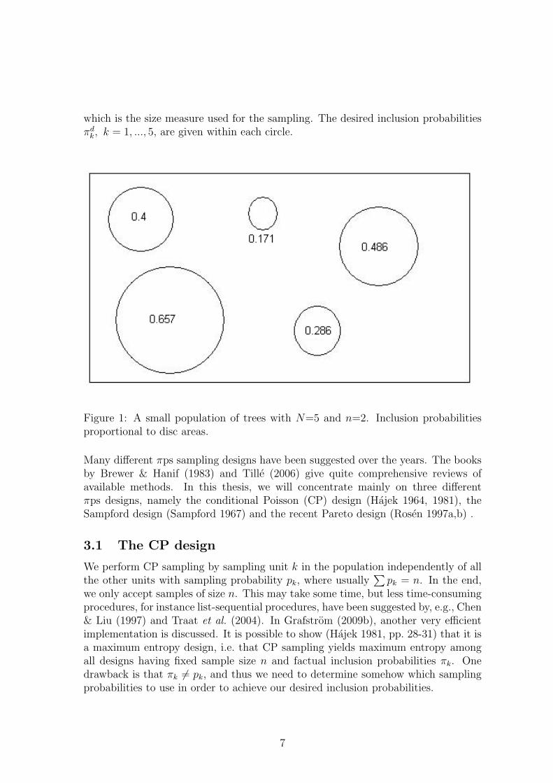
which is the size measure used for the sampling. The desired inclusion probabilitiesπd

k, k = 1, ..., 5, are given within each circle.

Figure 1: A small population of trees with N=5 and n=2. Inclusion probabilitiesproportional to disc areas.

Many different πps sampling designs have been suggested over the years. The booksby Brewer & Hanif (1983) and Tille (2006) give quite comprehensive reviews ofavailable methods. In this thesis, we will concentrate mainly on three differentπps designs, namely the conditional Poisson (CP) design (Hajek 1964, 1981), theSampford design (Sampford 1967) and the recent Pareto design (Rosen 1997a,b) .

3.1 The CP design

We perform CP sampling by sampling unit k in the population independently of allthe other units with sampling probability pk, where usually

∑pk = n. In the end,

we only accept samples of size n. This may take some time, but less time-consumingprocedures, for instance list-sequential procedures, have been suggested by, e.g., Chen& Liu (1997) and Traat et al. (2004). In Grafstrom (2009b), another very efficientimplementation is discussed. It is possible to show (Hajek 1981, pp. 28-31) that it isa maximum entropy design, i.e. that CP sampling yields maximum entropy amongall designs having fixed sample size n and factual inclusion probabilities πk. Onedrawback is that πk 6= pk, and thus we need to determine somehow which samplingprobabilities to use in order to achieve our desired inclusion probabilities.

7

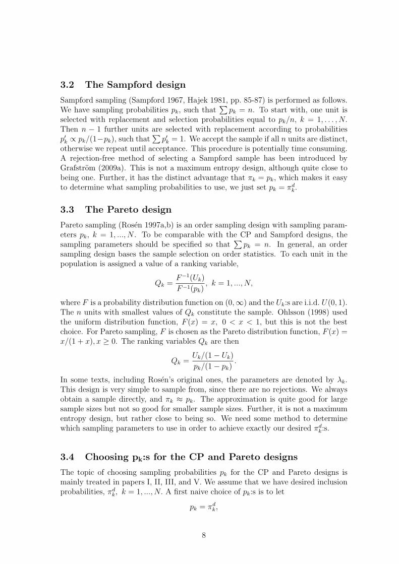
3.2 The Sampford design

Sampford sampling (Sampford 1967, Hajek 1981, pp. 85-87) is performed as follows.We have sampling probabilities pk, such that

∑pk = n. To start with, one unit is

selected with replacement and selection probabilities equal to pk/n, k = 1, . . . , N.Then n − 1 further units are selected with replacement according to probabilitiesp′k ∝ pk/(1−pk), such that

∑p′k = 1. We accept the sample if all n units are distinct,

otherwise we repeat until acceptance. This procedure is potentially time consuming.A rejection-free method of selecting a Sampford sample has been introduced byGrafstrom (2009a). This is not a maximum entropy design, although quite close tobeing one. Further, it has the distinct advantage that πk = pk, which makes it easyto determine what sampling probabilities to use, we just set pk = πd

k.

3.3 The Pareto design

Pareto sampling (Rosen 1997a,b) is an order sampling design with sampling param-eters pk, k = 1, ..., N . To be comparable with the CP and Sampford designs, thesampling parameters should be specified so that

∑pk = n. In general, an order

sampling design bases the sample selection on order statistics. To each unit in thepopulation is assigned a value of a ranking variable,

Qk =F−1(Uk)

F−1(pk), k = 1, ..., N,

where F is a probability distribution function on (0,∞) and the Uk:s are i.i.d. U(0, 1).The n units with smallest values of Qk constitute the sample. Ohlsson (1998) usedthe uniform distribution function, F (x) = x, 0 < x < 1, but this is not the bestchoice. For Pareto sampling, F is chosen as the Pareto distribution function, F (x) =x/(1 + x), x ≥ 0. The ranking variables Qk are then

Qk =Uk/(1− Uk)

pk/(1− pk).

In some texts, including Rosen’s original ones, the parameters are denoted by λk.This design is very simple to sample from, since there are no rejections. We alwaysobtain a sample directly, and πk ≈ pk. The approximation is quite good for largesample sizes but not so good for smaller sample sizes. Further, it is not a maximumentropy design, but rather close to being so. We need some method to determinewhich sampling parameters to use in order to achieve exactly our desired πd

k:s.

3.4 Choosing pk:s for the CP and Pareto designs

The topic of choosing sampling probabilities pk for the CP and Pareto designs ismainly treated in papers I, II, III, and V. We assume that we have desired inclusionprobabilities, πd

k, k = 1, ..., N. A first naive choice of pk:s is to let

pk = πdk,

8

which unfortunately yields, for both designs, that

πk 6= πdk

and we introduce some bias in the HT-estimator. There are now two options: wecan use an analytical approach or a computer-intensive iterative approach, or acombination. The main contributions in this thesis are in the analytical field. Wehave the πd

k:s to work with, and it is reasonable to assume that there exist functions,f and g for CP and Pareto respectively, such that if we choose

pk = f(πdk, d) and pk = g(πd

k, d),

whered =

∑πd

k(1− πdk),

we will obtain almost correct inclusion probabilities, i.e. πk ≈ πdk, where the approx-

imation is very close. We need some idea about how to choose f and g. Further, itis in fact easier to work with the ”sampling odds”

rk = pk/(1− pk)

than with the pk:s themselves. In the first three papers we consider an asymptoticcase, namely the case where d is large. In paper I it is shown that in this asymptoticcase, the CP, Pareto and Sampford designs are equal from a probabilistic point ofview. We use this similarity in papers I, II, and III. In paper III, we also derivemeasures of the probabilistic distances between these designs, based on asymptoticconsiderations, and make some illustrations for a few cases. It is shown that thePareto design with adjusted pk:s is very close to the Sampford design. In paper V,we consider the CP design for the asymptotic case where d is close to zero. This is arather extreme case corresponding to, for a population ordered by decreasing desiredinclusion probabilities,

πdk ≈

1 k = 1, ..., n

0 k = n + 1, ..., N.

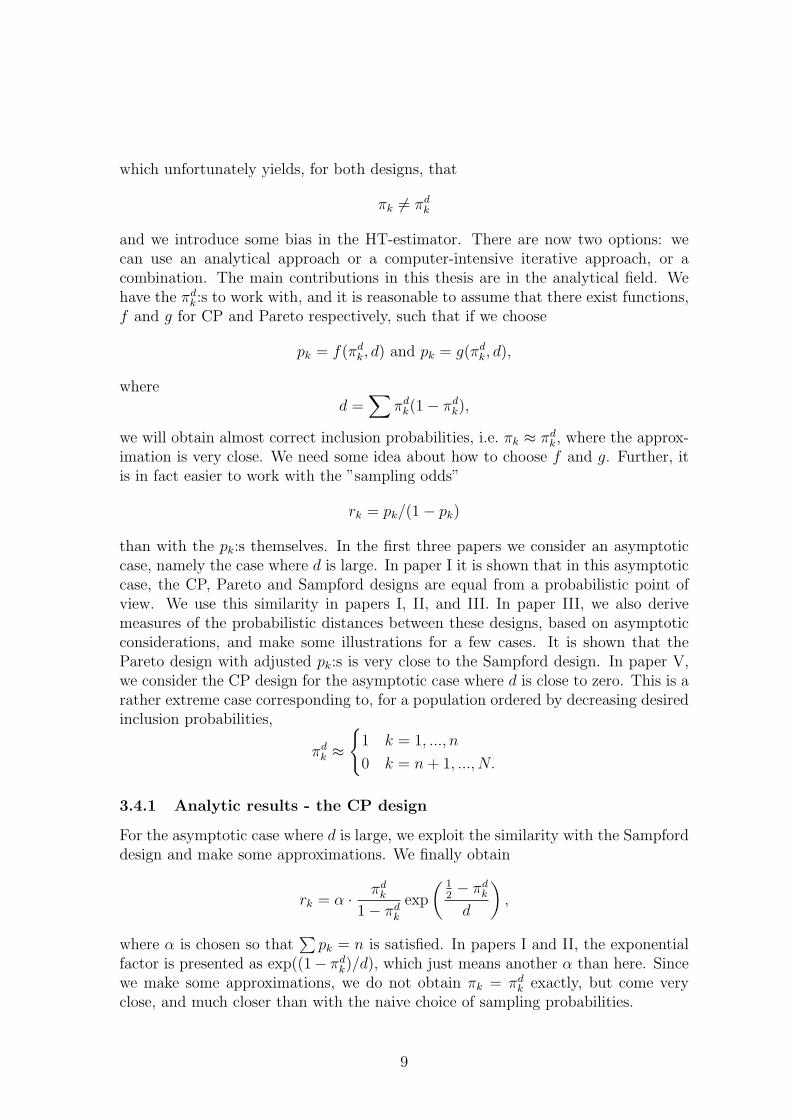
3.4.1 Analytic results - the CP design

For the asymptotic case where d is large, we exploit the similarity with the Sampforddesign and make some approximations. We finally obtain

rk = α · πdk

1− πdk

exp

( 12− πd

k

d

),

where α is chosen so that∑

pk = n is satisfied. In papers I and II, the exponentialfactor is presented as exp((1− πd

k)/d), which just means another α than here. Sincewe make some approximations, we do not obtain πk = πd

k exactly, but come veryclose, and much closer than with the naive choice of sampling probabilities.

9

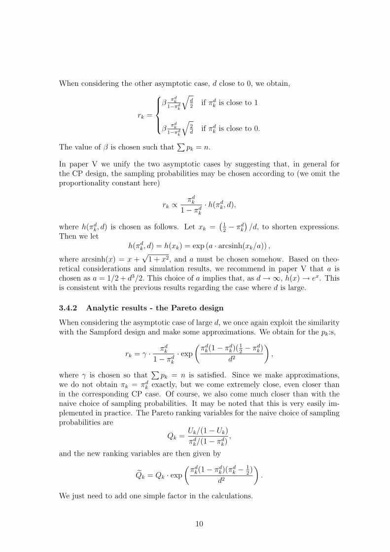
When considering the other asymptotic case, d close to 0, we obtain,

rk =

β

πdk

1−πdk

√d2

if πdk is close to 1

βπd

k

1−πdk

√2d

if πdk is close to 0.

The value of β is chosen such that∑

pk = n.

In paper V we unify the two asymptotic cases by suggesting that, in general forthe CP design, the sampling probabilities may be chosen according to (we omit theproportionality constant here)

rk ∝πd

k

1− πdk

· h(πdk, d),

where h(πdk, d) is chosen as follows. Let xk =

(12− πd

k

)/d, to shorten expressions.

Then we leth(πd

k, d) = h(xk) = exp (a · arcsinh(xk/a)) ,

where arcsinh(x) = x +√

1 + x2, and a must be chosen somehow. Based on theo-retical considerations and simulation results, we recommend in paper V that a ischosen as a = 1/2 + d3/2. This choice of a implies that, as d →∞, h(x) → ex. Thisis consistent with the previous results regarding the case where d is large.

3.4.2 Analytic results - the Pareto design

When considering the asymptotic case of large d, we once again exploit the similaritywith the Sampford design and make some approximations. We obtain for the pk:s,

rk = γ · πdk

1− πdk

· exp

(πd

k(1− πdk)(

12− πd

k)

d2

),

where γ is chosen so that∑

pk = n is satisfied. Since we make approximations,we do not obtain πk = πd

k exactly, but we come extremely close, even closer thanin the corresponding CP case. Of course, we also come much closer than with thenaive choice of sampling probabilities. It may be noted that this is very easily im-plemented in practice. The Pareto ranking variables for the naive choice of samplingprobabilities are

Qk =Uk/(1− Uk)

πdk/(1− πd

k),

and the new ranking variables are then given by

Qk = Qk · exp

(πd

k(1− πdk)(π

dk − 1

2)

d2

).

We just need to add one simple factor in the calculations.

10

For the asymptotic case where d is close to zero, we have no analytical results forthe Pareto design. It is suggested in paper V that the earlier function h may be usedad hoc for the Pareto design, replacing the xk:s with

yk = xk ·(

πdk(1− πd

k)

d

),

with xk as before. Some initial numerical experiments suggest that the πk:s are closerto the πd

k:s compared to the naive choice of sampling probabilities. The improvementis most obvious when d is very small, about 0.4 or smaller. For d-values larger than1 the refined adjustment is of no importance.

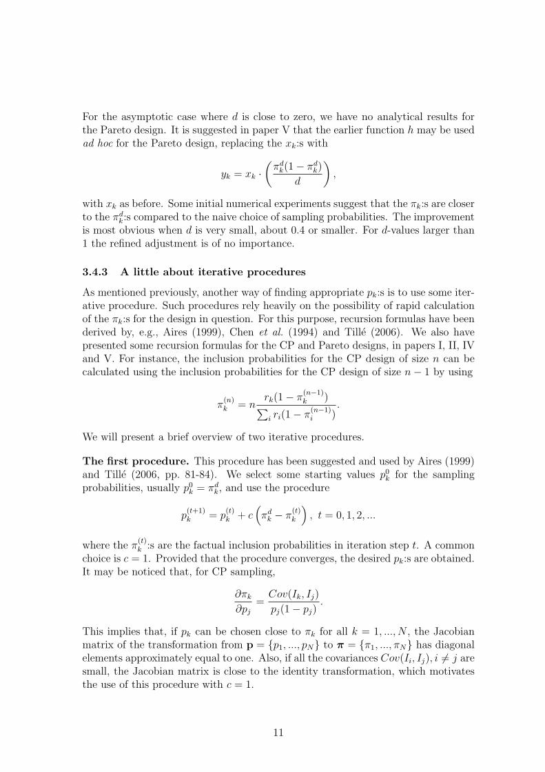
3.4.3 A little about iterative procedures

As mentioned previously, another way of finding appropriate pk:s is to use some iter-ative procedure. Such procedures rely heavily on the possibility of rapid calculationof the πk:s for the design in question. For this purpose, recursion formulas have beenderived by, e.g., Aires (1999), Chen et al. (1994) and Tille (2006). We also havepresented some recursion formulas for the CP and Pareto designs, in papers I, II, IVand V. For instance, the inclusion probabilities for the CP design of size n can becalculated using the inclusion probabilities for the CP design of size n− 1 by using

π(n)k = n

rk(1− π(n−1)k )∑

i ri(1− π(n−1)i )

.

We will present a brief overview of two iterative procedures.

The first procedure. This procedure has been suggested and used by Aires (1999)and Tille (2006, pp. 81-84). We select some starting values p0

k for the samplingprobabilities, usually p0

k = πdk, and use the procedure

p(t+1)k = p

(t)k + c

(πd

k − π(t)k

), t = 0, 1, 2, ...

where the π(t)k :s are the factual inclusion probabilities in iteration step t. A common

choice is c = 1. Provided that the procedure converges, the desired pk:s are obtained.It may be noticed that, for CP sampling,

∂πk

∂pj

=Cov(Ik, Ij)

pj(1− pj).

This implies that, if pk can be chosen close to πk for all k = 1, ..., N , the Jacobianmatrix of the transformation from p = p1, ..., pN to π = π1, ..., πN has diagonalelements approximately equal to one. Also, if all the covariances Cov(Ii, Ij), i 6= j aresmall, the Jacobian matrix is close to the identity transformation, which motivatesthe use of this procedure with c = 1.

11

The second procedure. Another possible choice is iterative proportional fitting.Here we let

p(t+1)k

1− p(t+1)k

=πd

k/(1− πdk)

π(t)k /(1− π

(t)k )

· p(t)k

1− p(t)k

, t = 0, 1, 2, ... ,

which illustrates how the name was chosen. For this procedure Chen et al. (1994)prove convergence for fixed size CP sampling. However, the procedure may be appliedfor Pareto sampling as well.

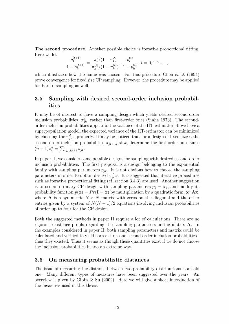
3.5 Sampling with desired second-order inclusion probabil-ities

It may be of interest to have a sampling design which yields desired second-orderinclusion probabilities, πd

jk, rather than first-order ones (Sinha 1973). The second-order inclusion probabilities appear in the variance of the HT-estimator. If we have asuperpopulation model, the expected variance of the HT-estimator can be minimizedby choosing the πd

jk:s properly. It may be noticed that for a design of fixed size n the

second-order inclusion probabilities πdjk, j 6= k, determine the first-order ones since

(n− 1)πdk =

∑j, j 6=k πd

jk.

In paper II, we consider some possible designs for sampling with desired second-orderinclusion probabilities. The first proposal is a design belonging to the exponentialfamily with sampling parameters pjk. It is not obvious how to choose the samplingparameters in order to obtain desired πd

jk:s. It is suggested that iterative proceduressuch as iterative proportional fitting (cf. section 3.4.3) are used. Another suggestionis to use an ordinary CP design with sampling parameters pk = πd

k, and modify itsprobability function p(x) = Pr(I = x) by multiplication by a quadratic form, xTAx,where A is a symmetric N × N matrix with zeros on the diagonal and the otherentries given by a system of N(N − 1)/2 equations involving inclusion probabilitiesof order up to four for the CP design.

Both the suggested methods in paper II require a lot of calculations. There are norigorous existence proofs regarding the sampling parameters or the matrix A. Inthe examples considered in paper II, both sampling parameters and matrix could becalculated and verified to yield correct first and second-order inclusion probabilities -thus they existed. Thus it seems as though these quantities exist if we do not choosethe inclusion probabilities in too an extreme way.

3.6 On measuring probabilistic distances

The issue of measuring the distance between two probability distributions is an oldone. Many different types of measures have been suggested over the years. Anoverview is given by Gibbs & Su (2002). Here we will give a short introduction ofthe measures used in this thesis.

12

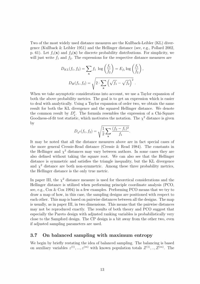
Two of the most widely used distance measures are the Kullback-Leibler (KL) diver-gence (Kullback & Leibler 1951) and the Hellinger distance (see, e.g., Pollard 2002,p. 61). Let f1(x) and f2(x) be discrete probability distributions. For simplicity, wewill just write f1 and f2. The expressions for the respective distance measures are

DKL(f1, f2) =∑x

f1 log

(f1

f2

)= Ef1 log

(f1

f2

),

DH(f1, f2) =

√2 ·

∑x

(√f1 −

√f2

)2

.

When we take asymptotic considerations into account, we use a Taylor expansion ofboth the above probability metrics. The goal is to get an expression which is easierto deal with analytically. Using a Taylor expansion of order two, we obtain the sameresult for both the KL divergence and the squared Hellinger distance. We denotethe common result by D2

χ. The formula resembles the expression of a Chi-SquareGoodness-of-fit test statistic, which motivates the notation. The χ2 distance is givenby

Dχ2(f1, f2) =

√1

2

∑x

(f2 − f1)2

f1

.

It may be noted that all the distance measures above are in fact special cases ofthe more general Cressie-Read distance (Cressie & Read 1984). The constants inthe Hellinger and χ2 distances may vary between authors. In some cases they arealso defined without taking the square root. We can also see that the Hellingerdistance is symmetric and satisfies the triangle inequality, but the KL divergenceand χ2 distance are both non-symmetric. Among these three probability metrics,the Hellinger distance is the only true metric.

In paper III, the χ2 distance measure is used for theoretical considerations and theHellinger distance is utilized when performing principle coordinate analysis (PCO,see, e.g., Cox & Cox 1994) in a few examples. Performing PCO means that we try todraw a map of how, in this case, the sampling designs are positioned with respect toeach other. This map is based on pairwise distances between all the designs. The mapis usually, as in paper III, in two dimensions. This means that the pairwise distancesmay not be reproduced exactly. The results of both theory and PCO suggest thatespecially the Pareto design with adjusted ranking variables is probabilistically veryclose to the Sampford design. The CP design is a bit away from the other two, evenif adjusted sampling parameters are used.

3.7 On balanced sampling with maximum entropy

We begin by briefly restating the idea of balanced sampling. The balancing is basedon auxiliary variables z(1), ..., z(m) with known population totals Z(1), .., Z(m). The

13

balancing conditions are ∑k∈s

dkz(j)k = Z(j), j = 1, ...,m,

for all samples s such that p(s) > 0. Only samples satisfying the balancing conditionsare given a positive probability of being selected.

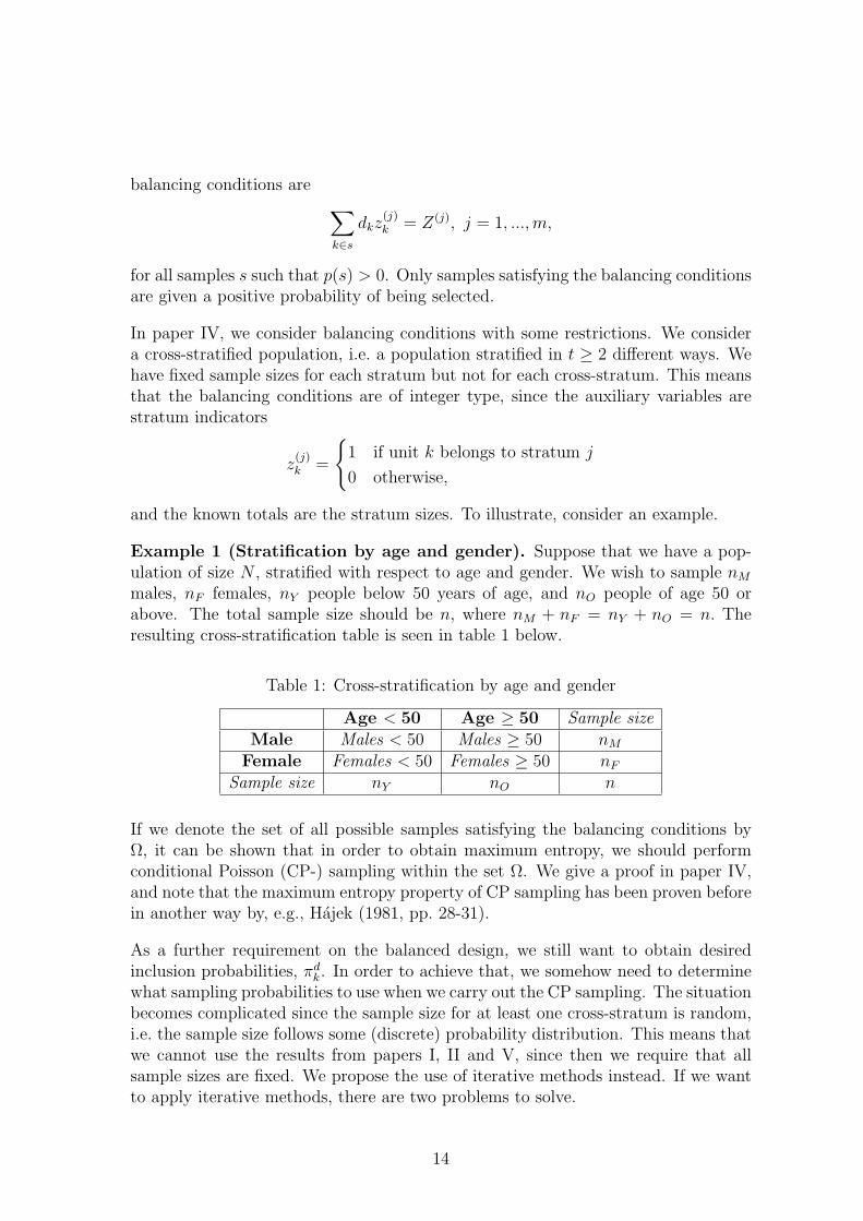
In paper IV, we consider balancing conditions with some restrictions. We considera cross-stratified population, i.e. a population stratified in t ≥ 2 different ways. Wehave fixed sample sizes for each stratum but not for each cross-stratum. This meansthat the balancing conditions are of integer type, since the auxiliary variables arestratum indicators

z(j)k =

1 if unit k belongs to stratum j

0 otherwise,

and the known totals are the stratum sizes. To illustrate, consider an example.

Example 1 (Stratification by age and gender). Suppose that we have a pop-ulation of size N , stratified with respect to age and gender. We wish to sample nM

males, nF females, nY people below 50 years of age, and nO people of age 50 orabove. The total sample size should be n, where nM + nF = nY + nO = n. Theresulting cross-stratification table is seen in table 1 below.

Table 1: Cross-stratification by age and gender

Age < 50 Age ≥ 50 Sample sizeMale Males < 50 Males ≥ 50 nM

Female Females < 50 Females ≥ 50 nF

Sample size nY nO n

If we denote the set of all possible samples satisfying the balancing conditions byΩ, it can be shown that in order to obtain maximum entropy, we should performconditional Poisson (CP-) sampling within the set Ω. We give a proof in paper IV,and note that the maximum entropy property of CP sampling has been proven beforein another way by, e.g., Hajek (1981, pp. 28-31).

As a further requirement on the balanced design, we still want to obtain desiredinclusion probabilities, πd

k. In order to achieve that, we somehow need to determinewhat sampling probabilities to use when we carry out the CP sampling. The situationbecomes complicated since the sample size for at least one cross-stratum is random,i.e. the sample size follows some (discrete) probability distribution. This means thatwe cannot use the results from papers I, II and V, since then we require that allsample sizes are fixed. We propose the use of iterative methods instead. If we wantto apply iterative methods, there are two problems to solve.

14

1. We need to calculate the probability distribution for the sample sizes.

2. For all possible sample sizes in each cross-stratum, we must calculate the ac-tual inclusion probabilities given the sample size in the cross-stratum and thesampling probabilities.

The first problem turns out to be computationally challenging. The required prob-ability functions may be written down explicitly, but in practice the number ofcombinations for which calculations need to be done grows rapidly. For very smallexamples, however, we can calculate the probability function exactly by using theexpression for it. For more realistic situations, we propose the use of Markov ChainMonte Carlo (MCMC) techniques, or Gaussian approximations, as a way of obtain-ing approximations to the distribution in question. The MCMC procedures are verygeneral and may be used in almost any possible setting. Further, we advocate thepossibility of using MCMC methods for sample selection as well. Currently MCMCmethods are not widely used in sampling theory. Now, once the first problem statedabove has been solved, we can solve the second one by combining the solution to thefirst problem with our previously known recursion formulas for CP sampling. Wecan thus use some iterative procedure to determine the sampling probabilities.

There is then the question if there always exists a sampling design that yields desiredinclusion probabilities πd

k satisfying∑

k∈S πdk = nS, where S denotes a stratum and

nS the stratum sample size, for each stratum. We give, in paper IV, such a proof forthe case of no more than three balancing conditions. For the case of four balancingconditions, we present a counterexample to show that in general there is no guaranteethat an appropriate sampling design exists.

4 Summary of the papers

Note that in the summaries of the papers, the notation has been adapted to becoherent with the rest of the introduction. The notation in the actual papers maydiffer somewhat from notation used here in the summaries.

4.1 Paper I. Pareto sampling versus Sampford and condi-tional Poisson sampling

In this paper we first compare the Pareto and Sampford sampling designs. We usetheir respective probability functions and Laplace approximations, and show thatfrom a probabilistic viewpoint these two designs are very close to each other. Infact, they can be shown to be asymptotically identical. The rejective method ofSampford sampling may be time consuming. We show that a Sampford sample maybe generated by passing a Pareto sample through an acceptance−rejection filter. Itis still a rejective method, but the number of rejections are reduced substantially.Most often, there are no rejections at all. This technique can be modified to give

15

us an efficient method to generate conditional Poisson (CP) samples as well. Wealso show how to calculate inclusion probabilities of any order for the Pareto designgiven the inclusion probabilities for the CP design. Finally, we derive a new explicitapproximation of the second-order inclusion probabilities. The new approximation isvalid for several designs, and we show how to apply it to get single sum type varianceestimates of the Horvitz-Thompson estimator.

4.2 Paper II. On sampling with desired inclusion probabili-ties of first and second order

We present a new simple approximation for obtaining sampling probabilities pk forconditional Poisson sampling to yield given inclusion probabilities πd

k. This approx-imation is based on the fact that the Sampford design yields the desired inclusionprobabilities. We present a few alternative routines to calculate exact pk-values, andcarry out some numerical comparisons. Further we derive two methods for achievingdesired second-order inclusion probabilities πd

jk. This might be interesting if we wantto control (and minimize) the variance of the Horvitz-Thompson estimator. Thefirst method is to use an exponential family probability function. We determine theparameters of this probability function by using an iterative proportional fitting al-gorithm. The second method we use is to modify the conditional Poisson probabilityfunction with a quadratic factor. We perform a small numerical study on these twomethods as well.

4.3 Paper III. On the distance between some πps samplingdesigns

Here, we derive an approximation for obtaining sampling parameters pk for Paretosampling in order to obtain given inclusion probabilities πd

k. We continue by inves-tigating the distances between some probability distributions arising from differentπps sampling designs. The designs in question are Poisson, Conditional Poisson(CP), Sampford, Pareto, Adjusted CP (cf. Paper II), and Adjusted Pareto sampling,as derived in this paper. We begin by using the Kullback-Leibler divergence and theHellinger distance. Then we use a Taylor expansion of order two on both distancemeasures. The common result is a simpler distance measure to work with theoreti-cally. This measure of χ2-type is evaluated first theoretically and then numerically inexamples with small populations. We further illustrate the numerical examples by amultidimensional scaling technique called principal coordinate analysis (PCO). Fromboth the theoretical analysis and the illustrated examples we see that Adjusted CP,Sampford, and adjusted Pareto are rather close to each other. In particular, Samp-ford and adjusted Pareto are very close. Pareto is located slightly further away fromthese, while CP and especially Poisson are quite far from all the others.

16

4.4 Paper IV. Balanced unequal probability sampling withmaximum entropy

We investigate how to perform balanced unequal probability sampling with maximumentropy. We focus on some particular balancing conditions, namely the conditions ofhaving specified marginal sums of the sample sizes in a cross-stratification table, butunspecified sample sizes in each cross-stratum of the table. When only the marginalsums are fixed, the sample sizes for one or more cross-stratums in the table arerandom. In principle, it is possible to express the probability distribution for thosesample sizes explicitly. However, the computations quickly become difficult, exceptfor very small cases. It is crucial to determine the probability distribution somehow,otherwise we are not able to calculate the inclusion probabilities for the design. Wepropose the use of Markov Chain Monte Carlo (MCMC) methods for obtaining goodapproximations to the probability distributions in question. It is proposed that theMCMC methods are used for sample selection as well. As another alternative, weconsider large-sample Gaussian approximations. As usual when conditional Poissonsampling is used, the inclusion probabilities do not equal the sampling ones. Regard-less of which method one uses for distributional calculation, iterative procedures maybe used for obtaining sampling probabilities yielding inclusion probabilities very closeor equal to the specified ones. We suggest a few different such iterative methods.

4.5 Paper V. A note on choosing sampling probabilities forconditional Poisson sampling

In this paper, the starting point is conditional Poisson sampling, and the fact thatthe sampling probabilities and the factual inclusion probabilities are not identical,even if

∑pk = n. This is a problem. We present a new method for choosing

the sampling probabilities, which may be used under more general conditions thanpreviously suggested methods (cf. paper II). The new method uses only the desired,predetermined, inclusion probabilities πd

k and the number d =∑

πdk(1 − πd

k). Wethen compare the performance of this new method to other reasonable choices ofsampling probabilities. Finally we note that this new method could also be used asan ad hoc method for determining the parameters for Pareto sampling.

5 Conclusion and some open problems

This thesis is very much about the CP, Sampford and Pareto sampling designs. Theyhave been thoroughly compared both theoretically and with examples (Papers I, IIand III), and we have derived adjustments for the CP and Pareto designs in orderto obtain desired inclusion probabilities (Papers I,II and V for CP, paper III forPareto). In particular, the adjustment for Pareto sampling is quite simple to use.The adjusted Pareto design has been found to be probabilistically very close to theSampford design. We have considered the CP design in connection with balanced

17

maximum entropy sampling (Paper IV). It might seem strange, but there is stillmuch more to be done. A few things will be mentioned below.

The area of balanced πps sampling has been introduced in the literature fairly re-cently, and there are plenty of things to do. For instance, the results about maximumentropy balanced sampling given in paper IV should be possible to generalize andextend quite a bit, both regarding existence of and how to determine the samplingprobabilities. The gaussian approximations could perhaps be replaced with someapproximate discrete probability distribution, since we are trying to approximate adiscrete distribution. The problem of finding a convenient and practical way of per-forming maximum entropy balanced sampling needs more attention. Possibly somegeneralization of Pareto sampling could be applied.

Regarding sampling with desired second-order inclusion probabilities a lot remainsto be done. There are theoretical problems, such as determining if a set of givenπd

jk:s really are second-order inclusion probabilities corresponding to some samplingdesign. There is also the problem of finding a practical way of performing the actualsampling. It is possible to use MCMC methods for sampling.

The analytical expressions for the sampling probabilities/parameters pk in CP andPareto sampling could possibly be improved, which will of course also be of benefitwhen applying iterative procedures, since we will have access to excellent startingvalues for the iterations. For the case where d is small an explicit expression for thepk:s, if such an expression even exists, has not yet been derived.

Finally, an issue which is not really a research problem. Considering the methods ofadjusting CP and Pareto sampling, they are not well known to the general samplingpublic. In particular the modification of Pareto sampling for large d is very simpleto use in practice, and for most populations found in practice, d is large enough tomake sure that the modification yields inclusion probabilities closer to the desiredones. Pareto sampling is one of the methods suggested by Statistics Sweden (2008)for performing πps sampling.

18

References

Aires, N. (1999). Algorithms to find exact inclusion probabilities for conditionalPoisson sampling and Pareto πps sampling designs. Methodol. Comput. Appl.Probab. 4, 457-469.

Bondesson, L. & Thorburn, D. (2008). A list sequential sampling method suitablefor real-time sampling. Scand. J. Statist. 35, 466-483.

Brewer, K.R.W. & Hanif, M. (1983). Sampling with unequal probabilities. LectureNotes in Statistics, No. 15. Springer-Verlag, New York.

Chen, S-X, Dempster, A.P. & Liu, J.S. (1994). Weighted finite population samplingto maximize entropy. Biometrika 81, 457-469.

Chen, S-X. & Liu, J.S. (1997). Statistical applications of the Poisson-binomial andconditional Bernoulli distributions. Statistica Sinica 7, 875-892.

Cox, T.F. & Cox, M.A.A. (1994). Multidimensional scaling. Chapman & Hall,London.

Cressie, N.A.C. & Read, T.R.C. (1984). Multinomial Goodness-of-fit tests. J. R.Statist. Soc. B. 46, 440-464.

Deville, J-C. & Sarndal, C-E. (1992). Calibration estimators in survey sampling. J.Amer. Statist. Assoc. 87, 376-382.

Gibbs, A.L. & Su, F.E. (2002). On choosing and bounding probability metrics.Internat. Statist. Rev. 70, 419-435.

Grafstrom, A. (2009a). Non-rejective implementations of the Sampford samplingdesign. J. Statist. Plann. Inference 139, 2111-2114.

Grafstrom, A. (2009b). Repeated Poisson sampling. Statist. Probab. Lett. 79, 760-764.

Hajek, J. (1964). Theory of rejective sampling. Ann. Math. Statist. 35, 1491-1523.

Hajek, J. (1981). Sampling from a finite population. Marcel Dekker, New York.

Holmberg, A. (2003). Essays on model assisted survey planning. PhD Thesis. De-partment of Information Sciences, Uppsala University.

Kullback, S. & Leibler, R.A. (1951). On information and sufficency. Ann. Math.Statist. 22, 79-86.

Meister, K. (2004). On methods for real time sampling and distributions in sampling.PhD Thesis. Department of Mathematical Statistics, Umea University.

Ohlsson, E. (1998) Sequential Poisson sampling. J. Off. Statist. 14, 149-162.

Pollard, David E. (2002). A user’s guide to measure theoretic probability. CambridgeUniversity Press, Cambridge, UK.

Rosen, B. (1997a). Asymptotic theory for order sampling. J. Statist. Plann. Infer-ence 62, 135-158.

19

Rosen, B. (1997b). On sampling with probability proportional to size. J. Statist.Plann. Inference 62, 159-191.

Sampford, M.R. (1967). On sampling without replacement with unequal probabili-ties of selection. Biometrika 54, 499-513.

Sinha, B.K. (1973). On sampling schemes to realize pre-assigned sets of inclusionprobabilities of the first two orders. Calcutta Statist. Assoc. Bull. 22, 89-110.

Statistics Sweden (2008) Urval - fran teori till praktik (Sampling, from theory topractice). Handbook 2008:1. Statistics Sweden, Stockholm.

Sarndal, C-E. & Lundstrom, S. (2005). Estimation in surveys with nonresponse.Wiley, Chichester.

Sarndal, C-E., Swensson, B. & Wretman, J. (1989). The weighted residual tech-nique for estimating the variance of the general regression estimator of the finitepopulation total. Biometrika. 76, 527-537.

Sarndal, C-E., Swensson, B. & Wretman, J. (1992). Model assisted survey sampling.Springer-Verlag, New York.

Tille, Y. (2006). Sampling algorithms. Springer science + Business media, Inc., NewYork.

Traat, I., Bondesson, L. & Meister, K. (2004). Sampling design and sample selectionthrough distribution theory. J. Statist. Plann. Inference 123, 395-413.

20