4. Basic probability theory
50
1 Lect04.ppt S-38.145 - Introduction to Teletraffic Theory – Spring 2005 4. Basic probability theory
Transcript of 4. Basic probability theory
1Lect04.ppt S-38.145 - Introduction to Teletraffic Theory – Spring 2005
4. Basic probability theory
2
4. Basic probability theory
Contents
• Basic concepts
• Discrete random variables
• Discrete distributions (nbr distributions)
• Continuous random variables
• Continuous distributions (time distributions)
• Other random variables
3
4. Basic probability theory
Sample space, sample points, events
• Sample space Ω is the set of all possible sample points ω ∈ Ω
– Example 0. Tossing a coin: Ω = H,T
– Example 1. Casting a die: Ω = 1,2,3,4,5,6
– Example 2. Number of customers in a queue: Ω = 0,1,2,...
– Example 3. Call holding time (e.g. in minutes): Ω = x ∈ ℜ | x > 0
• Events A,B,C,... ⊂ Ω are measurable subsets of the sample space Ω
– Example 1. “Even numbers of a die”: A = 2,4,6
– Example 2. “No customers in a queue”: A = 0
– Example 3. “Call holding time greater than 3.0 (min)”: A = x ∈ ℜ | x > 3.0
• Denote by the set of all events A ∈
– Sure event: The sample space Ω ∈ itself
– Impossible event: The empty set ∅ ∈
4
4. Basic probability theory
Combination of events
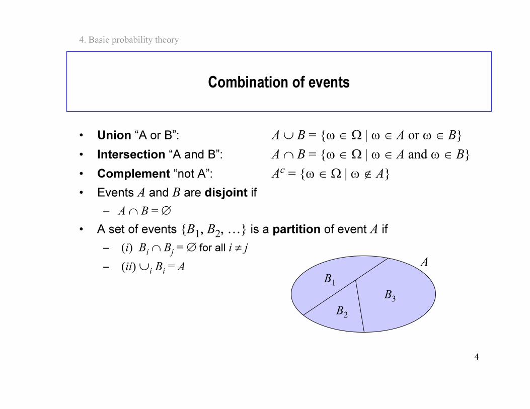
• Union “A or B”: A ∪ B = ω ∈ Ω | ω ∈ A or ω ∈ B
• Intersection “A and B”: A ∩ B = ω ∈ Ω | ω ∈ A and ω ∈ B
• Complement “not A”: Ac = ω ∈ Ω | ω ∉ A
• Events A and B are disjoint if
– A ∩ B = ∅
• A set of events B1, B
2, … is a partition of event A if
– (i) Bi ∩ Bj = ∅ for all i ≠ j
– (ii) ∪i Bi = AB1
B2
B3
A
5
4. Basic probability theory
Probability
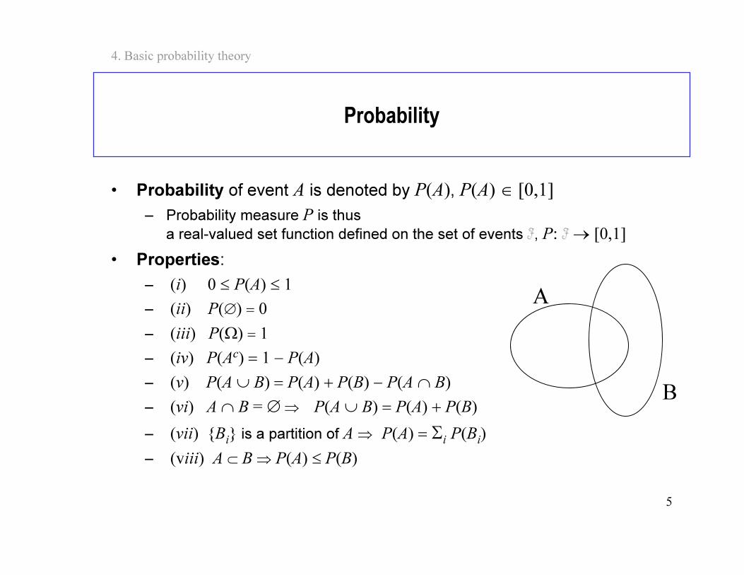
• Probability of event A is denoted by P(A), P(A) ∈ [0,1]
– Probability measure P is thus
a real-valued set function defined on the set of events , P: → [0,1]
• Properties:
– (i) 0 ≤ P(A) ≤ 1
– (ii) P(∅) = 0
– (iii) P(Ω) = 1
– (iv) P(Ac) = 1 − P(A)
– (v) P(A ∪ B) = P(A) + P(B) − P(A ∩ B)
– (vi) A ∩ B = ∅⇒ P(A ∪ B) = P(A) + P(B)
– (vii) Bi is a partition of A ⇒ P(A) = Σi P(Bi)
– (viii) A ⊂ B ⇒ P(A) ≤ P(B)
A
B
6
4. Basic probability theory
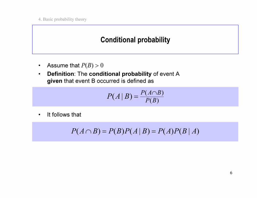
Conditional probability
• Assume that P(B) > 0
• Definition: The conditional probability of event A
given that event B occurred is defined as
• It follows that
)(
)()|(
BP
BAPBAP
∩
=
)|()()|()()( ABPAPBAPBPBAP ==∩
7
4. Basic probability theory
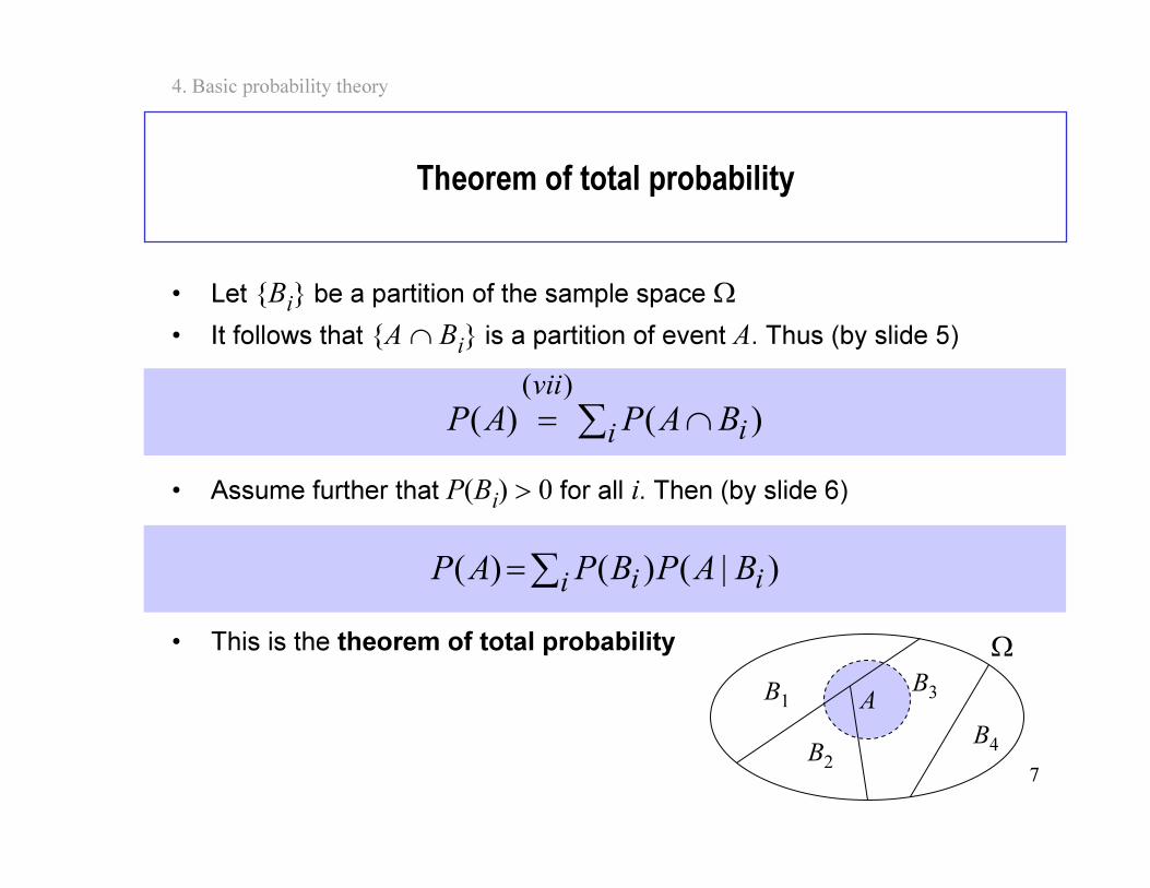
Theorem of total probability
• Let Bi be a partition of the sample space Ω
• It follows that A ∩ Bi is a partition of event A. Thus (by slide 5)
• Assume further that P(Bi) > 0 for all i. Then (by slide 6)
• This is the theorem of total probability
B1
B2
B3
B4
A
∑ ∩=i i
vii
BAPAP )()()(
Ω
∑= i ii BAPBPAP )|()()(
8
4. Basic probability theory
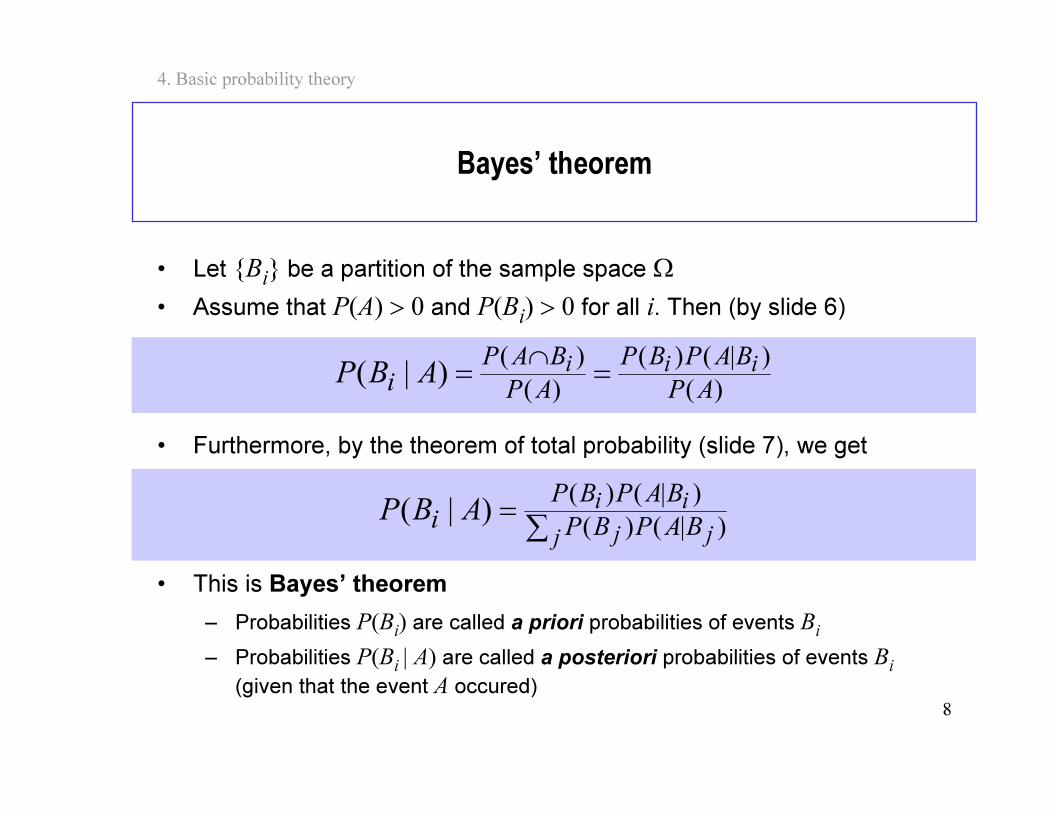
Bayes’ theorem
• Let Bi be a partition of the sample space Ω
• Assume that P(A) > 0 and P(Bi) > 0 for all i. Then (by slide 6)
• Furthermore, by the theorem of total probability (slide 7), we get
• This is Bayes’ theorem
– Probabilities P(Bi) are called a priori probabilities of events B
i
– Probabilities P(Bi | A) are called a posteriori probabilities of events B
i
(given that the event A occured)
)(
)|()(
)(
)()|(
AP
BAPBP
AP
BAP
iiii
ABP ==
∩
∑=
j jj
ii
BAPBP
BAPBP
i ABP)|()(
)|()()|(
9
4. Basic probability theory
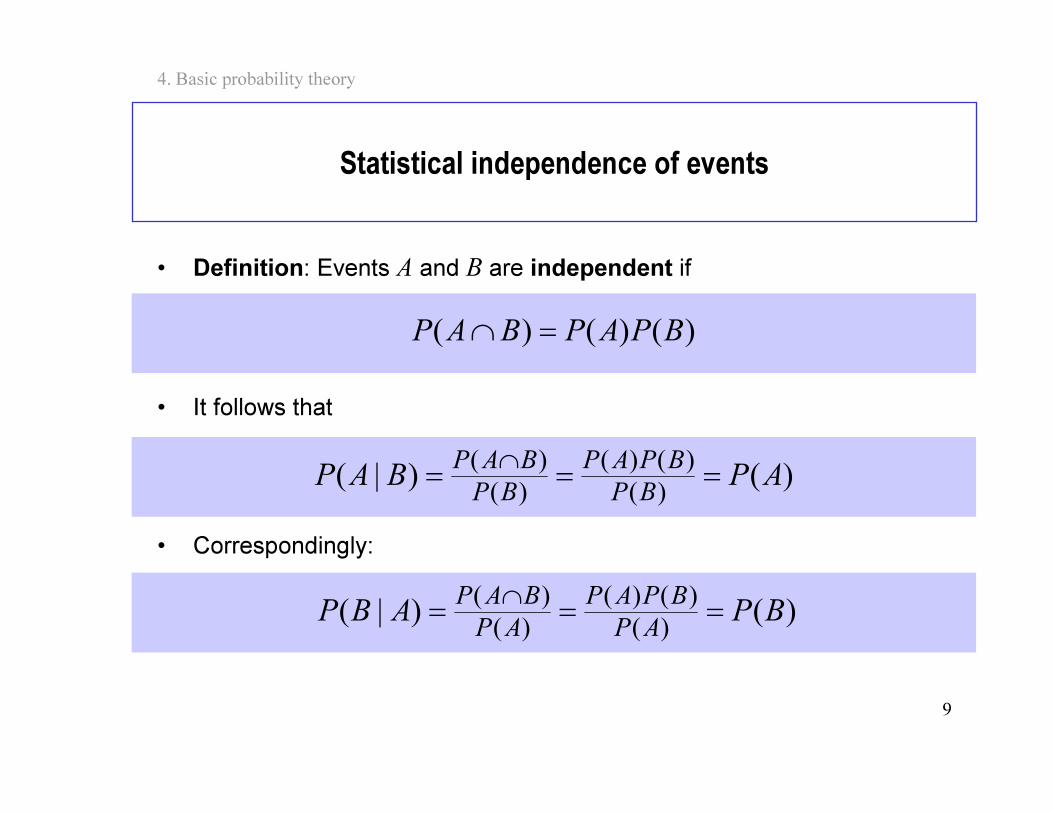
Statistical independence of events
• Definition: Events A and B are independent if
• It follows that
• Correspondingly:
)()()( BPAPBAP =∩
)()|()(
)()(
)(
)(APBAP
BP
BPAP
BP
BAP===
∩
)()|()(
)()(
)(
)(BPABP
AP
BPAP
AP
BAP===
∩
10
4. Basic probability theory
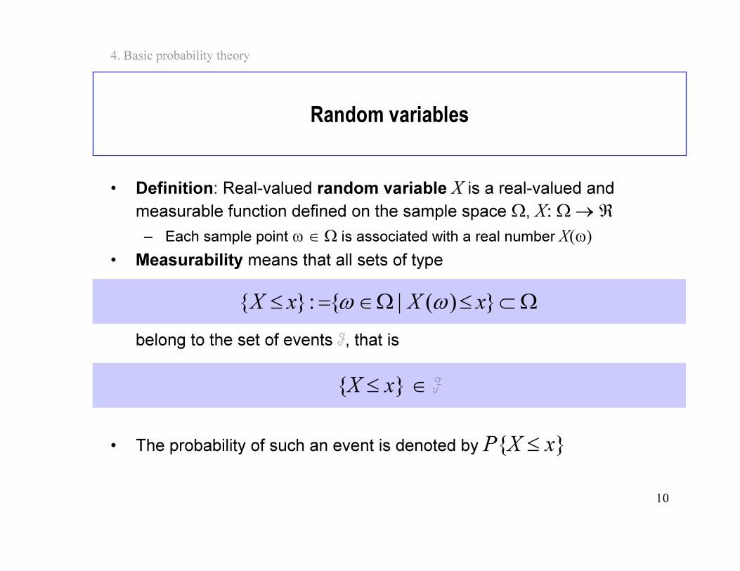
• Definition: Real-valued random variable X is a real-valued and
measurable function defined on the sample space Ω, X: Ω→ ℜ
– Each sample point ω ∈ Ω is associated with a real number X(ω)
• Measurability means that all sets of type
belong to the set of events , that is
X ≤ x ∈
• The probability of such an event is denoted by PX ≤ x
Random variables
Ω⊂≤Ω∈=≤ )(|: xXxX ωω
11
4. Basic probability theory
Example
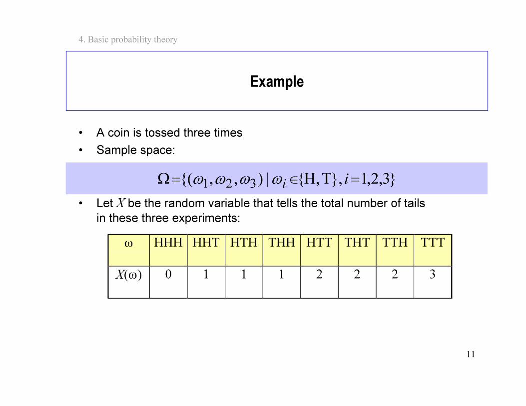
• A coin is tossed three times
• Sample space:
• Let X be the random variable that tells the total number of tails in these three experiments:
3,2,1,T,H|),,( 321 =∈=Ω iiωωωω
ω HHH HHT HTH THH HTT THT TTH TTT
X(ω) 0 1 1 1 2 2 2 3
12
4. Basic probability theory
Indicators of events
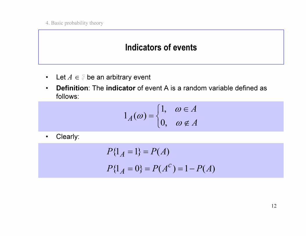
• Let A ∈ be an arbitrary event
• Definition: The indicator of event A is a random variable defined as
follows:
• Clearly:
∉
∈=
A
A
Aω
ω
ω
,0
,1)(1
)(1)(01
)(11
APAPP
APP
cA
A
−===
==
13
4. Basic probability theory
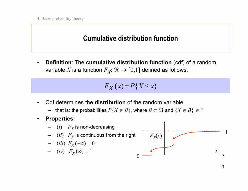
• Definition: The cumulative distribution function (cdf) of a random
variable X is a function FX: ℜ→ [0,1] defined as follows:
• Cdf determines the distribution of the random variable,
– that is: the probabilities PX ∈ B, where B ⊂ ℜ and X ∈ B ∈
• Properties:
– (i) FXis non-decreasing
– (ii) FXis continuous from the right
– (iii) FX (−∞) = 0
– (iv) FX (∞) = 1
Cumulative distribution function
)( xXPxFX ≤=
FX(x)
x
0
1
14
4. Basic probability theory
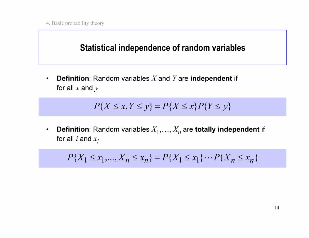
Statistical independence of random variables
• Definition: Random variables X and Y are independent if
for all x and y
• Definition: Random variables X1,…, X
nare totally independent if
for all i and xi
, yYPxXPyYxXP ≤≤=≤≤
,..., 1111 nnnnxXPxXPxXxXP ≤≤=≤≤ L
15
4. Basic probability theory
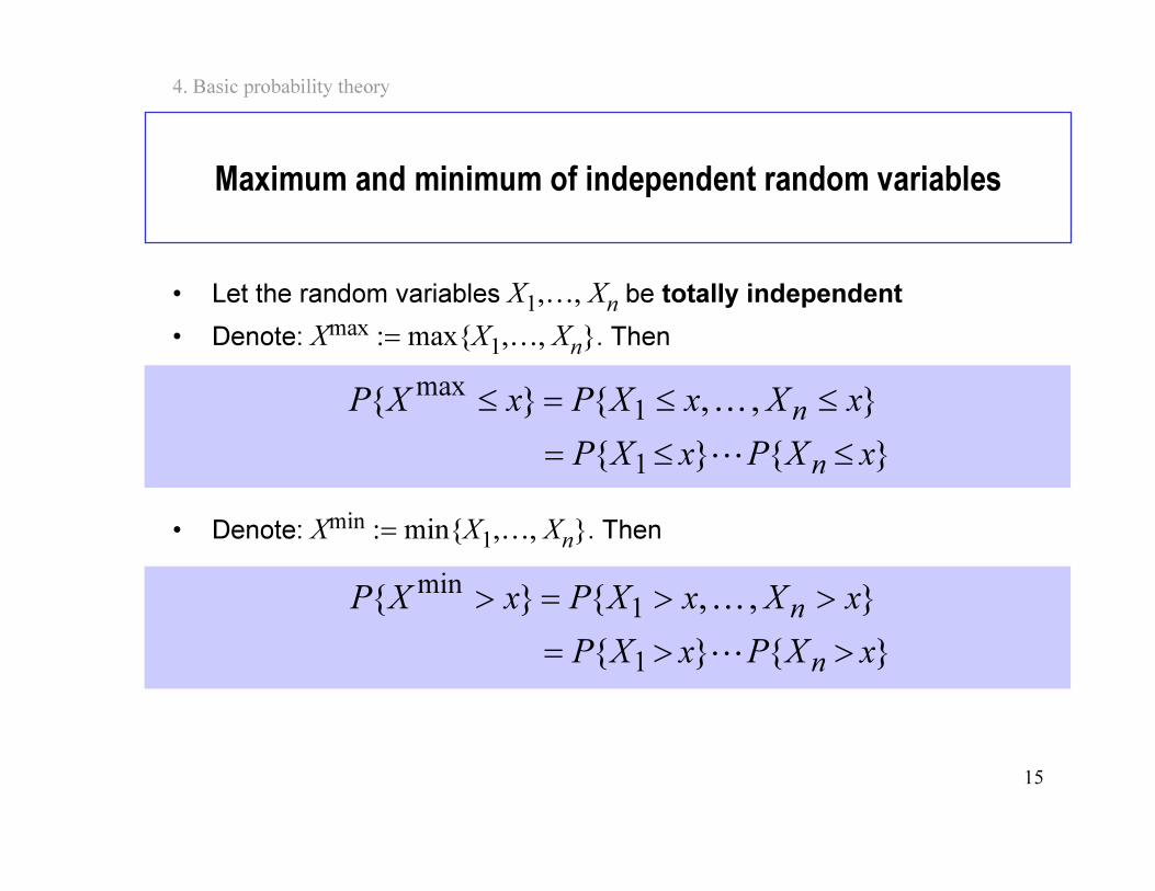
Maximum and minimum of independent random variables
• Let the random variables X1,…, X
nbe totally independent
• Denote: Xmax := maxX1,…, X
n. Then
• Denote: Xmin := minX1,…, X
n. Then
, , 1max
xXxXPxXPn≤≤=≤ K
1 xXPxXPn≤≤= L
, , 1min
xXxXPxXPn>>=> K
1 xXPxXPn>>= L
16
4. Basic probability theory
Contents
• Basic concepts
• Discrete random variables
• Discrete distributions (nbr distributions)
• Continuous random variables
• Continuous distributions (time distributions)
• Other random variables
17
4. Basic probability theory
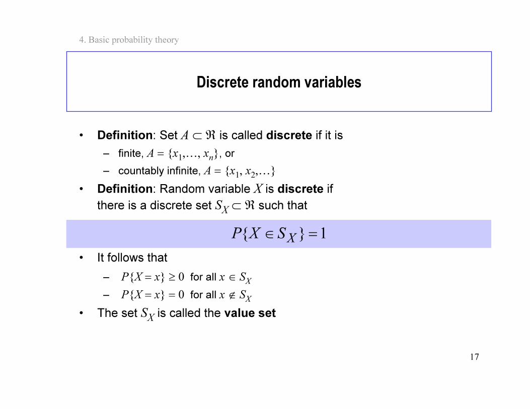
Discrete random variables
• Definition: Set A ⊂ ℜ is called discrete if it is
– finite, A = x1,…, x
n, or
– countably infinite, A = x1, x
2,…
• Definition: Random variable X is discrete if
there is a discrete set SX ⊂ ℜ such that
• It follows that
– PX = x ≥ 0 for all x ∈ SX
– PX = x = 0 for all x ∉ SX
• The set SX is called the value set
1 =∈ XSXP
18
4. Basic probability theory
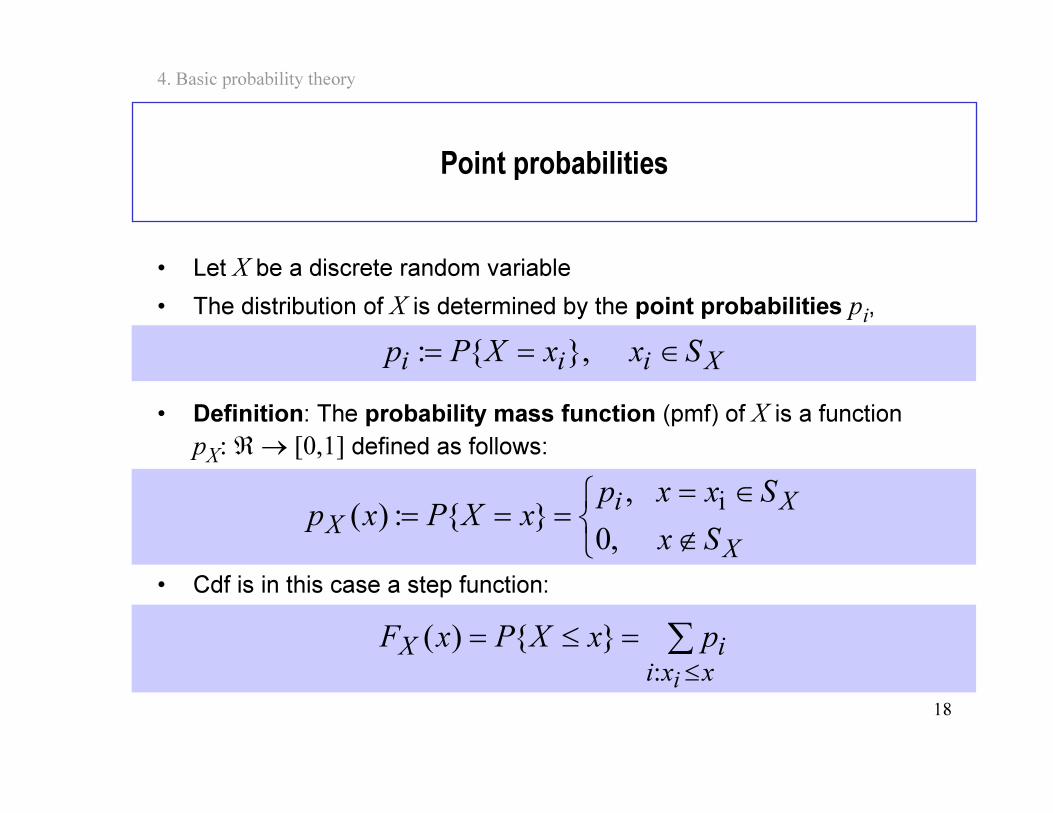
Point probabilities
• Let X be a discrete random variable
• The distribution of X is determined by the point probabilities pi,
• Definition: The probability mass function (pmf) of X is a function
pX: ℜ → [0,1] defined as follows:
• Cdf is in this case a step function:
Xiii SxxXPp ∈== ,:
∉
∈====
,0
,:)(
i
X
Xi
XSx
SxxpxXPxp
∑≤
=≤=
xxi
iX
i
pxXPxF:
)(
19
4. Basic probability theory
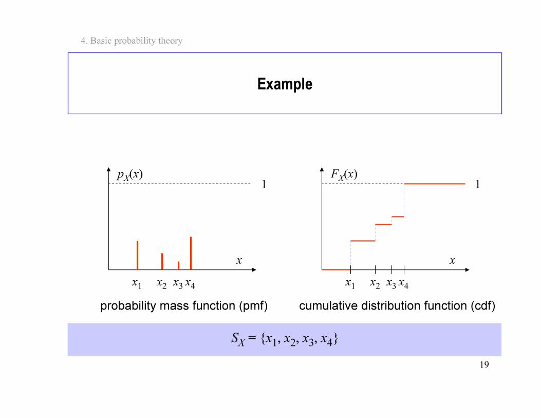
Example
x
pX(x)
probability mass function (pmf)
x
FX(x)
cumulative distribution function (cdf)
x1
x2x3x4
x1
x2x3x4
1 1
SX = x1, x2, x3, x4
20
4. Basic probability theory
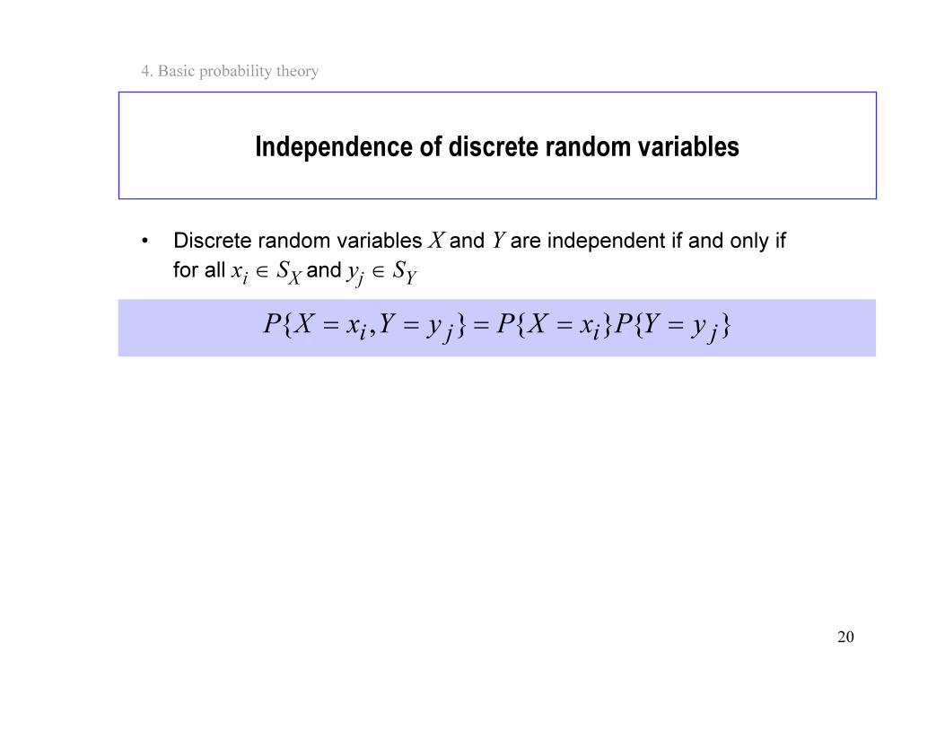
Independence of discrete random variables
• Discrete random variables X and Y are independent if and only if
for all xi ∈ SX and yj ∈ SY
, jiji yYPxXPyYxXP =====
21
4. Basic probability theory
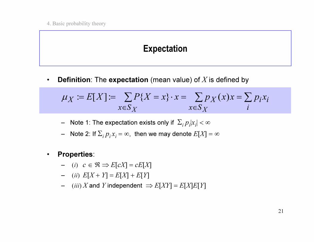
Expectation
• Definition: The expectation (mean value) of X is defined by
– Note 1: The expectation exists only if Σipi|xi| < ∞
– Note 2: If Σipi xi= ∞, then we may denote E[X] = ∞
• Properties:
– (i) c ∈ ℜ ⇒ E[cX] = cE[X]
– (ii) E[X + Y] = E[X] + E[Y]
– (iii) X and Y independent ⇒ E[XY] = E[X]E[Y]
∑∑∑ ==⋅===
∈∈ i
ii
Sx
X
Sx
X xpxxpxxXPXE
XX
)(:][:µ
22
4. Basic probability theory
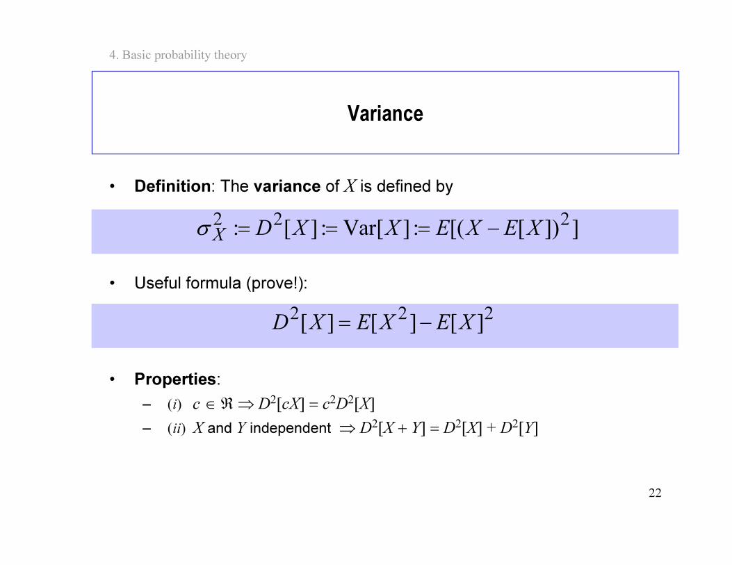
Variance
• Definition: The variance of X is defined by
• Useful formula (prove!):
• Properties:
– (i) c ∈ ℜ ⇒ D2[cX] = c2D2[X]
– (ii) X and Y independent ⇒ D2[X + Y] = D2[X] + D2[Y]
]])[[(:]Var[:][: 222XEXEXXDX −===σ
222][][][ XEXEXD −=
23
4. Basic probability theory
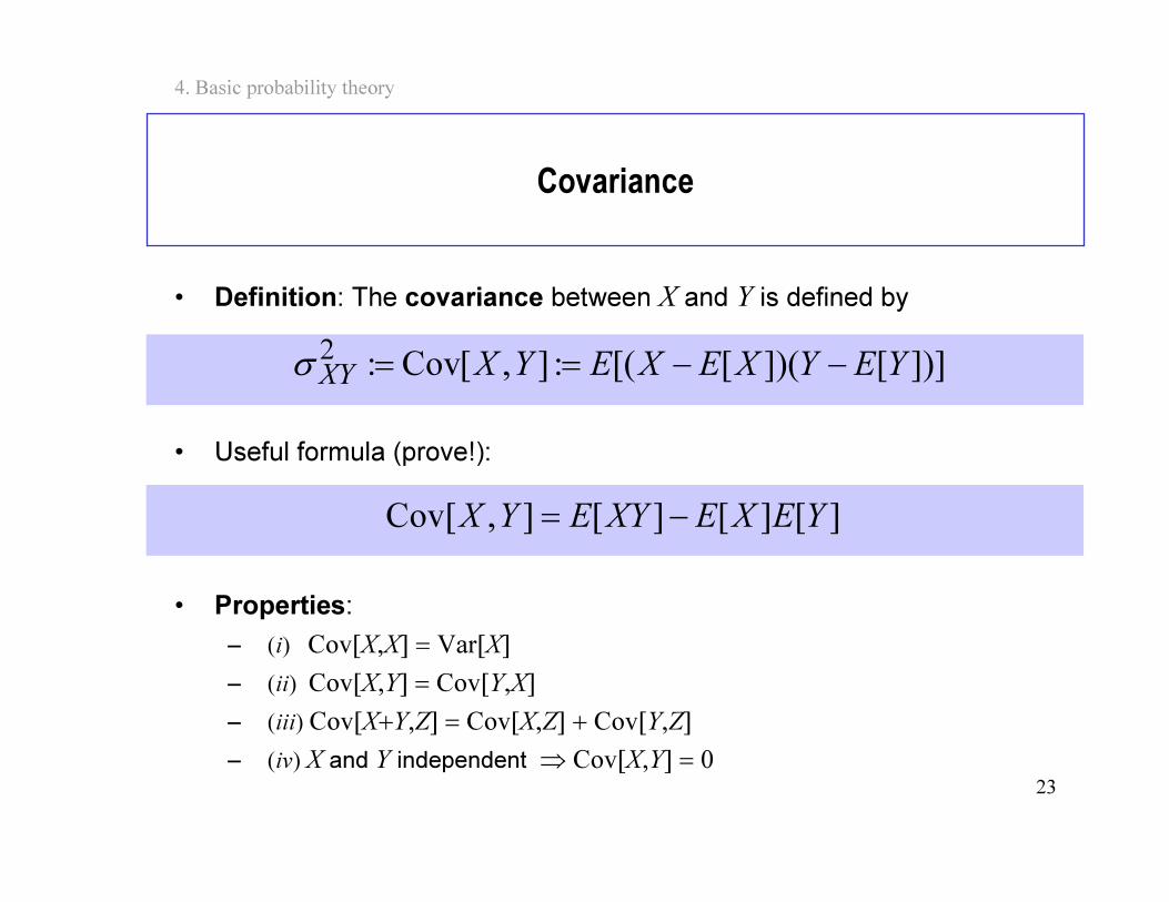
Covariance
• Definition: The covariance between X and Y is defined by
• Useful formula (prove!):
• Properties:
– (i) Cov[X,X] = Var[X]
– (ii) Cov[X,Y] = Cov[Y,X]
– (iii) Cov[X+Y,Z] = Cov[X,Z] + Cov[Y,Z]
– (iv) X and Y independent ⇒ Cov[X,Y] = 0
])][])([[(:],[Cov: 2YEYXEXEYXXY −−==σ
][][][],Cov[ YEXEXYEYX −=
24
4. Basic probability theory
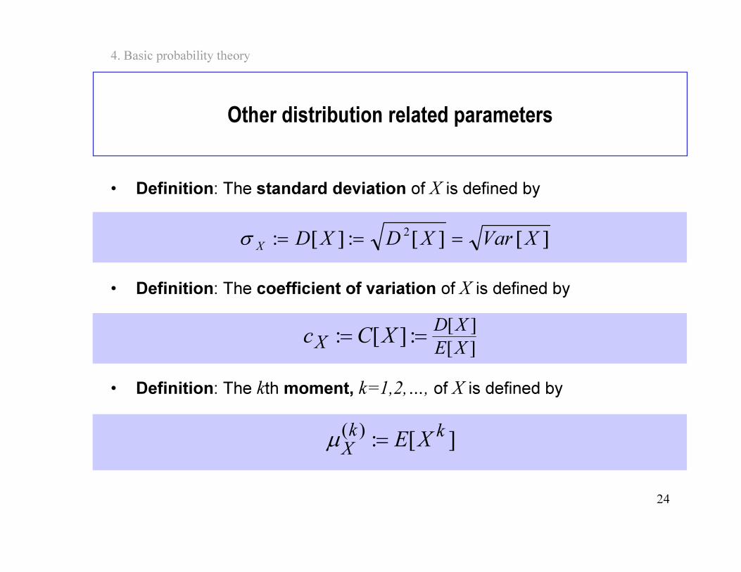
Other distribution related parameters
• Definition: The standard deviation of X is defined by
• Definition: The coefficient of variation of X is defined by
• Definition: The kth moment, k=1,2,…, of X is defined by
][][:][: 2
XVarXDXDX
===σ
][
][:][:
XE
XD
X XCc ==
][:)( kk
XXE=µ
25
4. Basic probability theory
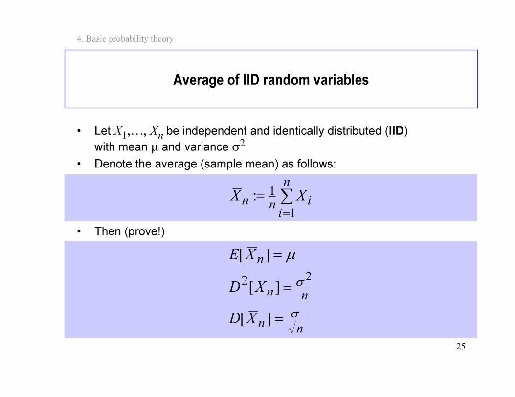
Average of IID random variables
• Let X1,…, Xn be independent and identically distributed (IID)
with mean µ and variance σ2
• Denote the average (sample mean) as follows:
• Then (prove!)
∑=
=
n
i
inn XX
1
1:
nn
nn
n
XD
XD
XE
σ
σ
µ
=
=
=
][
][
][
22
26
4. Basic probability theory
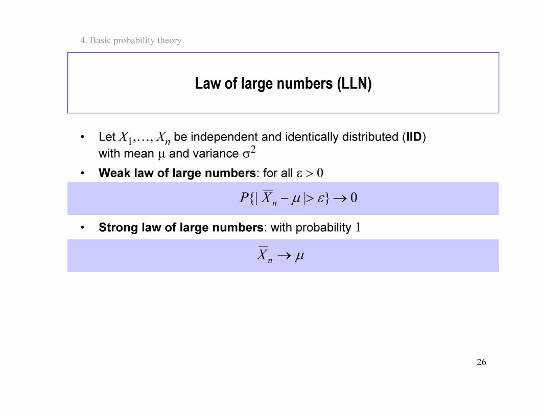
Law of large numbers (LLN)
• Let X1,…, Xn be independent and identically distributed (IID)
with mean µ and variance σ2
• Weak law of large numbers: for all ε > 0
• Strong law of large numbers: with probability 1
0|| →>− εµn
XP
µ→n
X
27
4. Basic probability theory
Contents
• Basic concepts
• Discrete random variables
• Discrete distributions (nbr distributions)
• Continuous random variables
• Continuous distributions (time distributions)
• Other random variables
28
4. Basic probability theory
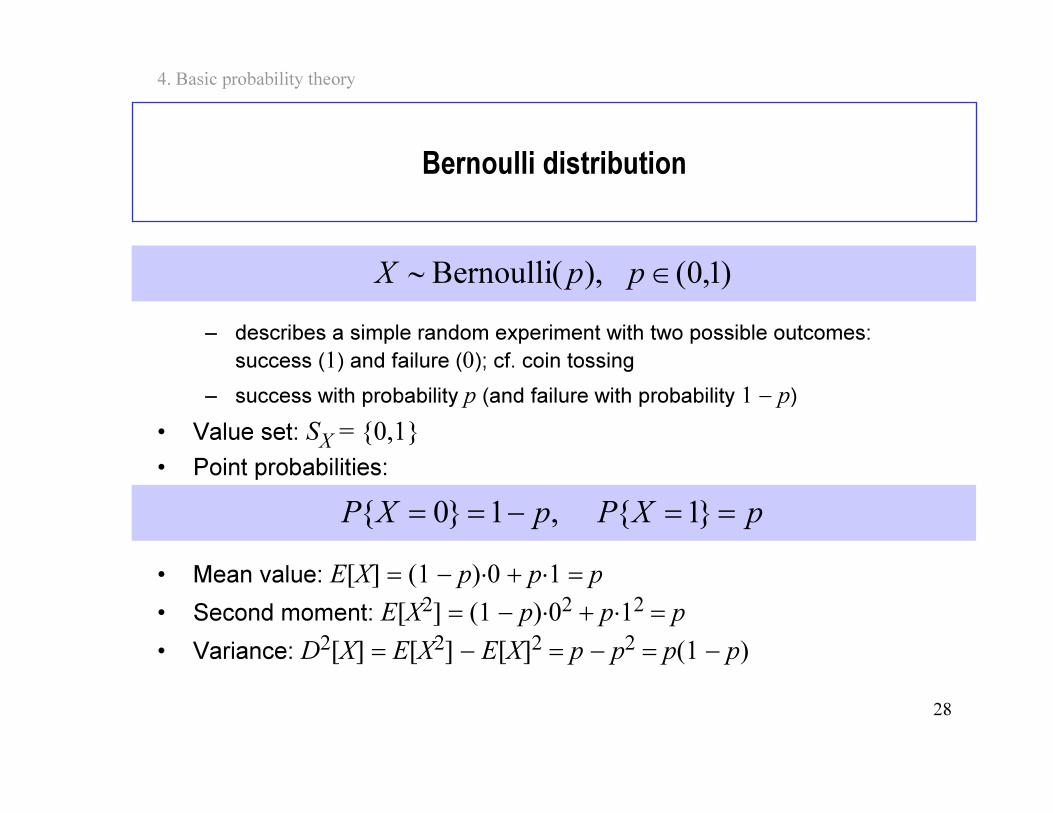
Bernoulli distribution
– describes a simple random experiment with two possible outcomes:
success (1) and failure (0); cf. coin tossing
– success with probability p (and failure with probability 1 − p)
• Value set: SX = 0,1
• Point probabilities:
• Mean value: E[X] = (1 − p)⋅0 + p⋅1 = p
• Second moment: E[X2] = (1 − p)⋅02 + p⋅12 = p
• Variance: D2[X] = E[X2] − E[X]2 = p − p2 = p(1 − p)
)1,0( ),(Bernoulli ∈∼ ppX
pXPpXP ==−== 1 ,10
29
4. Basic probability theory
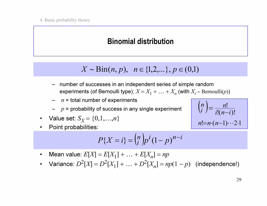
Binomial distribution
– number of successes in an independent series of simple random
experiments (of Bernoulli type); X = X1+… + X
n(with X
i∼ Bernoulli(p))
– n = total number of experiments
– p = probability of success in any single experiment
• Value set: SX = 0,1,…,n
• Point probabilities:
• Mean value: E[X] = E[X1] +… + E[Xn] = np
• Variance: D2[X] = D2[X1] +… + D2[Xn] = np(1 − p) (independence!)
)1,0(,...,2,1 ),,(Bin ∈∈∼ pnpnX
( ) inin
i ppiXP−
−== )1(
( )12)1(!
)!(!!
⋅−⋅=
−
=
Lnnn
ini
nn
i
30
4. Basic probability theory
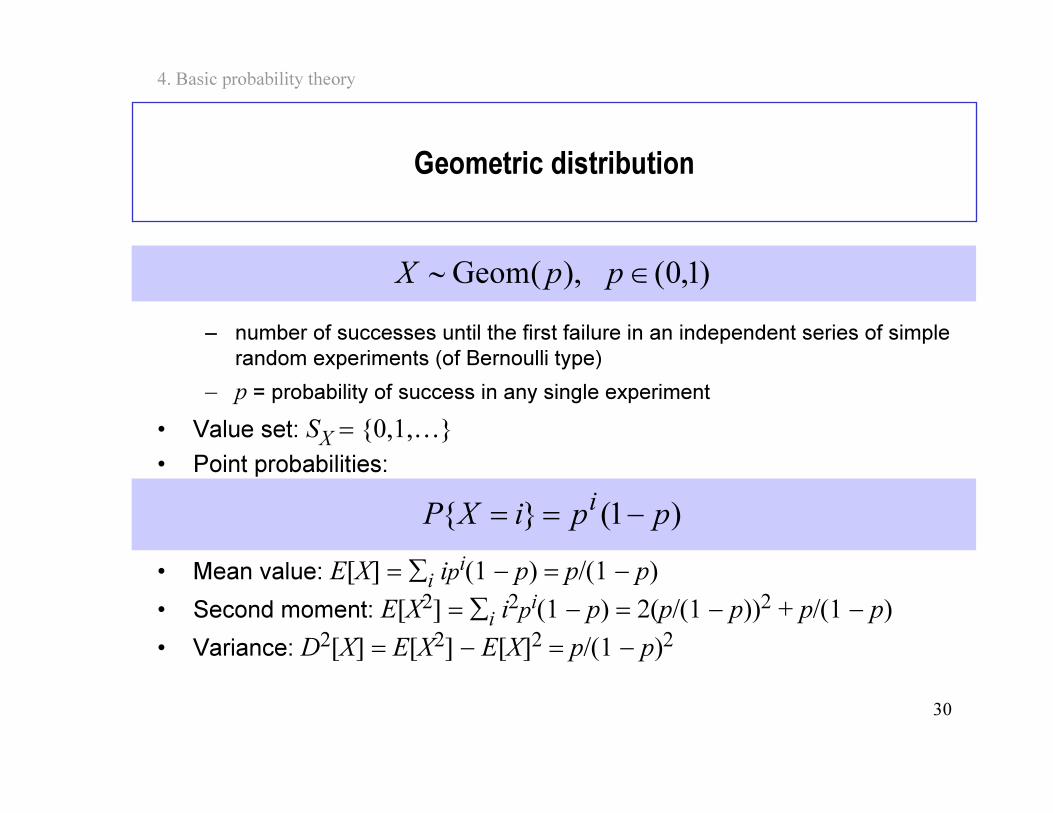
Geometric distribution
– number of successes until the first failure in an independent series of simple
random experiments (of Bernoulli type)
– p = probability of success in any single experiment
• Value set: SX = 0,1,…
• Point probabilities:
• Mean value: E[X] = ∑i ipi(1 − p) = p/(1 − p)
• Second moment: E[X2] = ∑i i2pi(1 − p) = 2(p/(1 − p))2 + p/(1 − p)
• Variance: D2[X] = E[X2] − E[X]2 = p/(1 − p)2
)1,0( ),(Geom ∈∼ ppX
)1( ppiXPi
−==
31
4. Basic probability theory
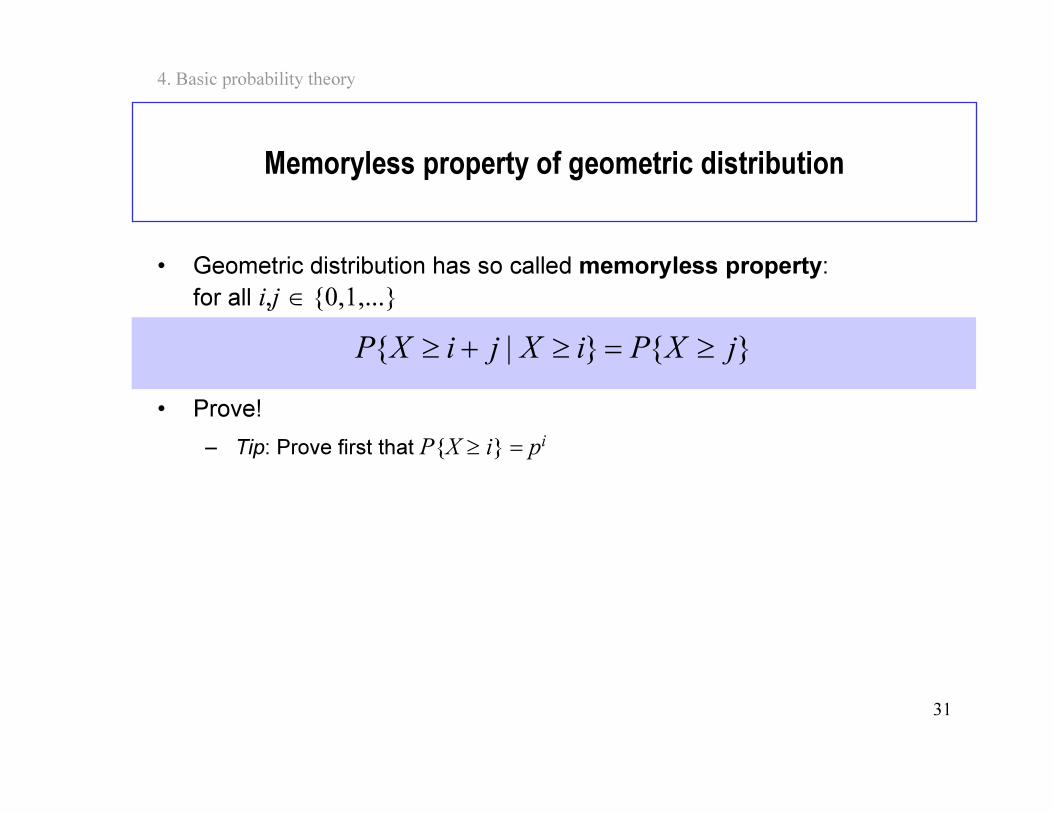
Memoryless property of geometric distribution
• Geometric distribution has so called memoryless property:
for all i,j ∈ 0,1,...
• Prove!
– Tip: Prove first that PX ≥ i = pi
| jXPiXjiXP ≥=≥+≥

32
4. Basic probability theory
Minimum of geometric random variables
• Let X1 ∼ Geom(p1) and X2 ∼ Geom(p2) be independent. Then
and
• Prove!
– Tip: See slide 15
)(Geom,min: 2121min
ppXXX ∼=
2,1 ,21 1
1min∈==
−
−
iXXPpp
pi
i
33
4. Basic probability theory
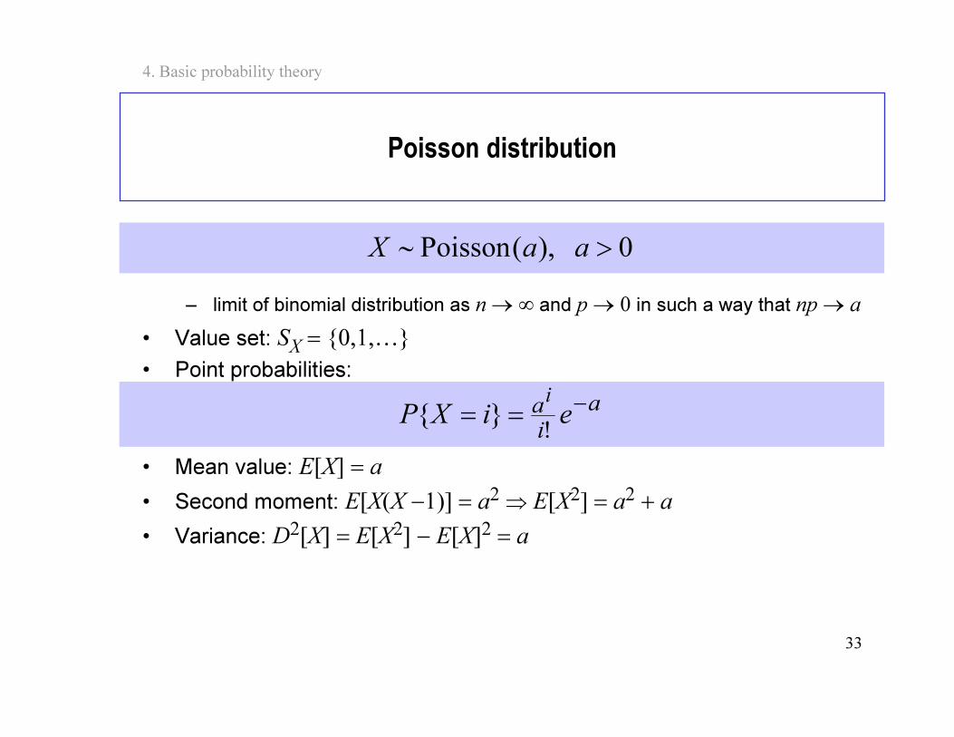
Poisson distribution
– limit of binomial distribution as n→ ∞ and p → 0 in such a way that np → a
• Value set: SX= 0,1,…
• Point probabilities:
• Mean value: E[X] = a
• Second moment: E[X(X −1)] = a2 ⇒ E[X2] = a2 + a
• Variance: D2[X] = E[X2] − E[X]2 = a
0 ),(Poisson >∼ aaX
a
i
aeiXP
i−
==
!
34
4. Basic probability theory
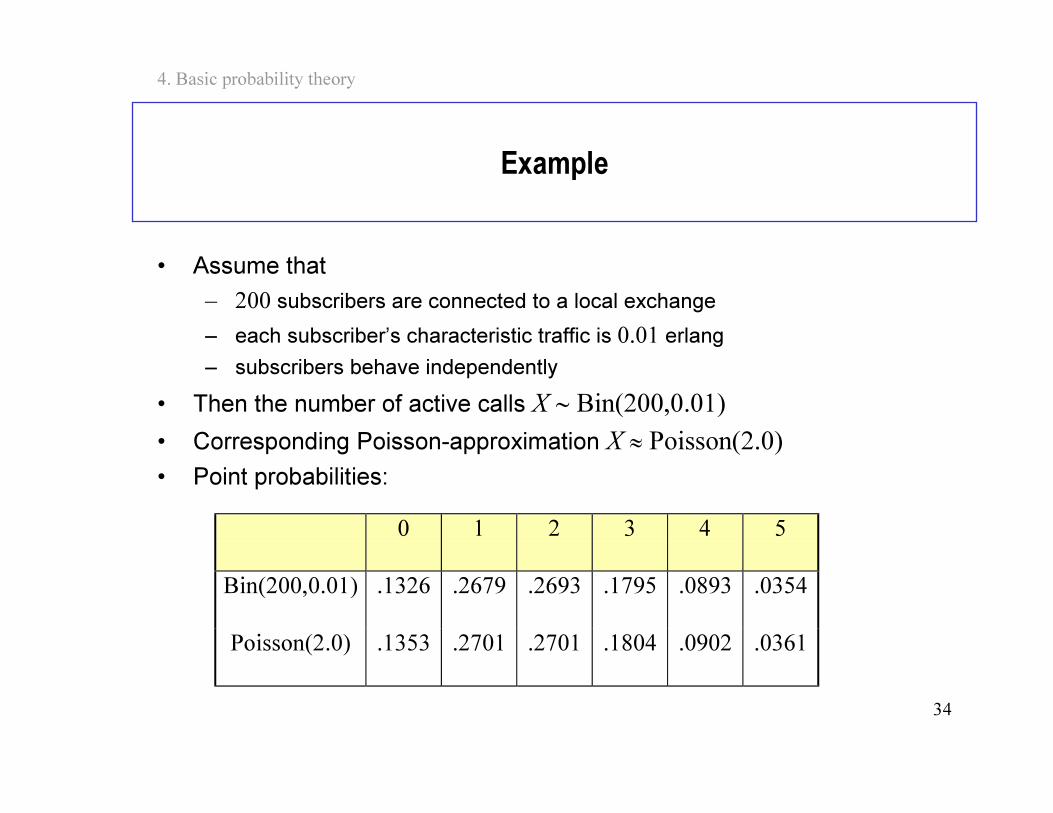
Example
• Assume that
– 200 subscribers are connected to a local exchange
– each subscriber’s characteristic traffic is 0.01 erlang
– subscribers behave independently
• Then the number of active calls X ∼ Bin(200,0.01)
• Corresponding Poisson-approximation X ≈ Poisson(2.0)
• Point probabilities:
0 1 2 3 4 5
Bin(200,0.01) .1326 .2679 .2693 .1795 .0893 .0354
Poisson(2.0) .1353 .2701 .2701 .1804 .0902 .0361
35
4. Basic probability theory
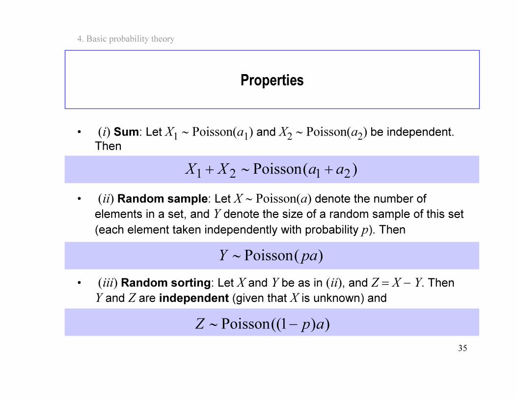
Properties
• (i) Sum: Let X1 ∼ Poisson(a1) and X2 ∼ Poisson(a2) be independent. Then
• (ii) Random sample: Let X ∼ Poisson(a) denote the number of
elements in a set, and Y denote the size of a random sample of this set
(each element taken independently with probability p). Then
• (iii) Random sorting: Let X and Y be as in (ii), and Z = X − Y. Then
Y and Z are independent (given that X is unknown) and
)(Poisson 2121 aaXX +∼+
)(Poisson paY ∼
))1((Poisson apZ −∼
36
4. Basic probability theory
Contents
• Basic concepts
• Discrete random variables
• Discrete distributions (nbr distributions)
• Continuous random variables
• Continuous distributions (time distributions)
• Other random variables
37
4. Basic probability theory
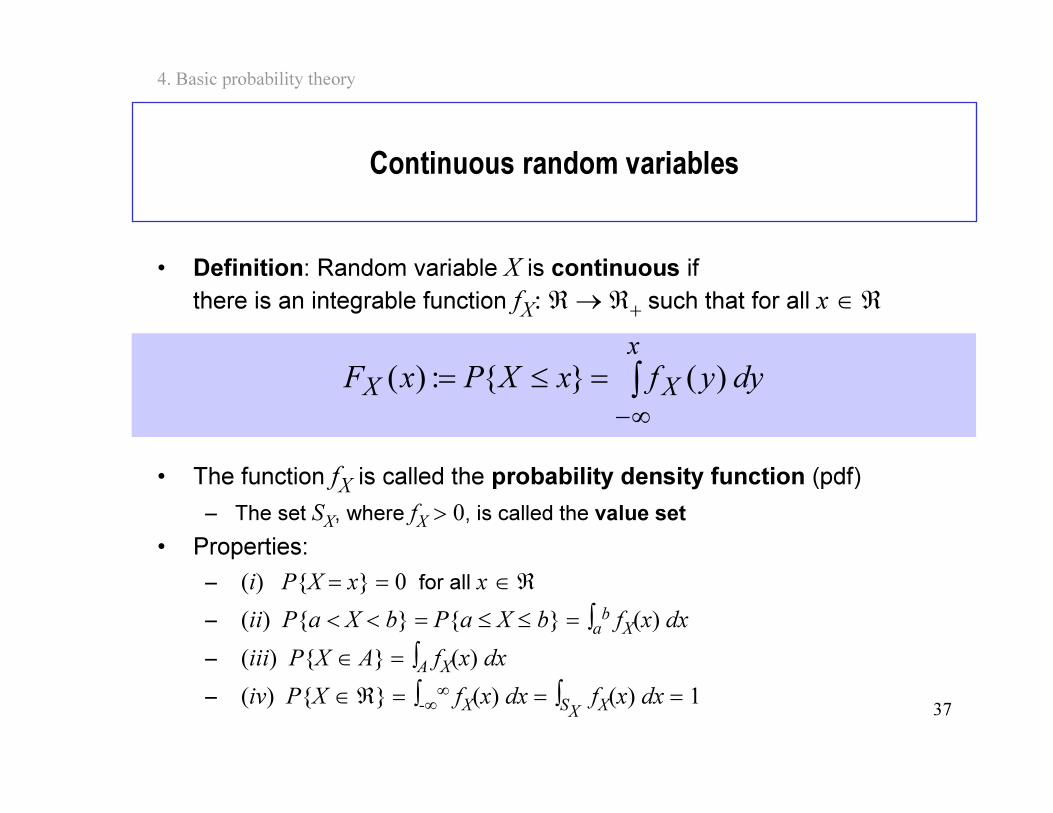
Continuous random variables
• Definition: Random variable X is continuous if
there is an integrable function fX: ℜ→ ℜ
+such that for all x ∈ ℜ
• The function fXis called the probability density function (pdf)
– The set SX, where f
X> 0, is called the value set
• Properties:
– (i) PX = x = 0 for all x ∈ ℜ
– (ii) Pa < X < b = Pa ≤ X ≤ b = ∫ab f
X(x) dx
– (iii) PX ∈ A = ∫AfX(x) dx
– (iv) PX ∈ ℜ = ∫-∞
∞ fX(x) dx = ∫
SXfX(x) dx = 1
∫∞−
=≤=
x
XX dyyfxXPxF )(:)(
38
4. Basic probability theory
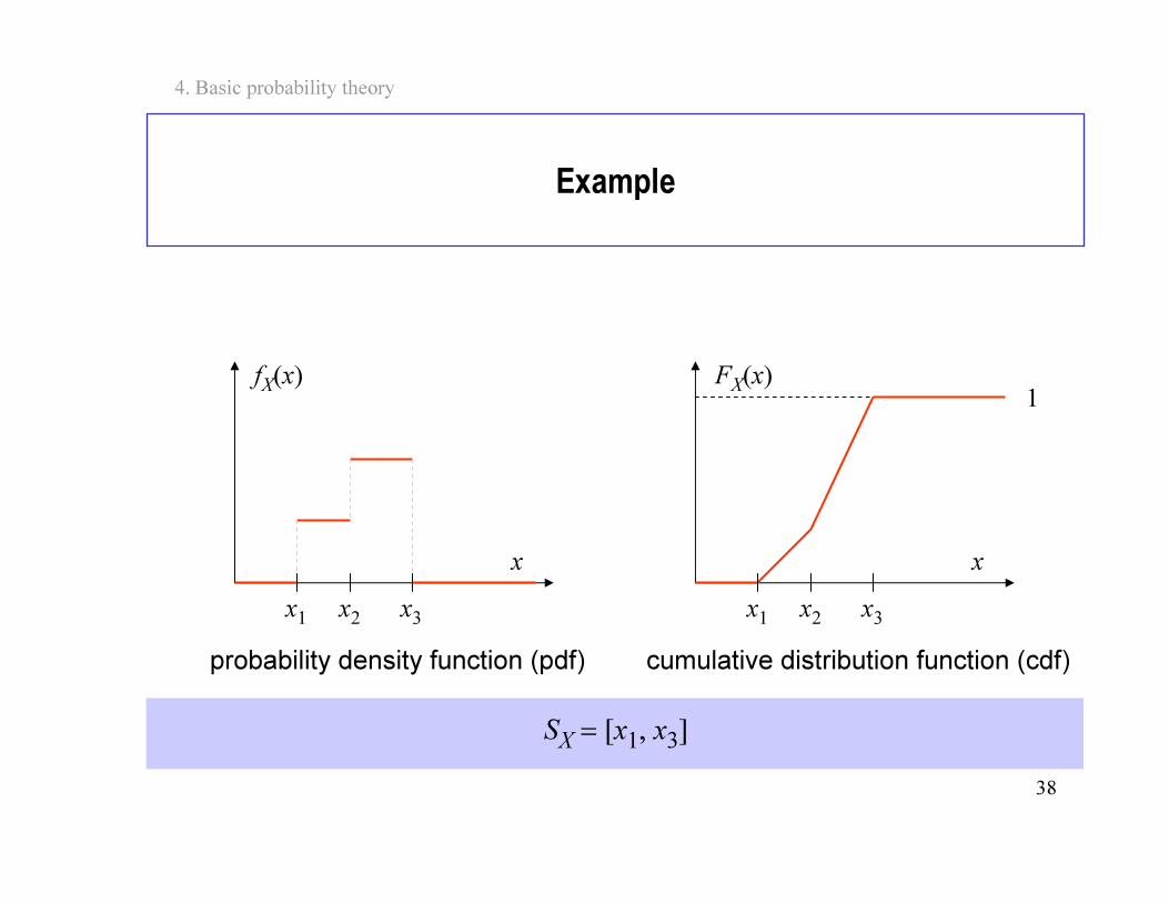
Example
x
fX(x)
probability density function (pdf)
x
FX(x)
cumulative distribution function (cdf)
x1
x2
x3
x1
x2
x3
1
SX= [x1, x3]
39
4. Basic probability theory
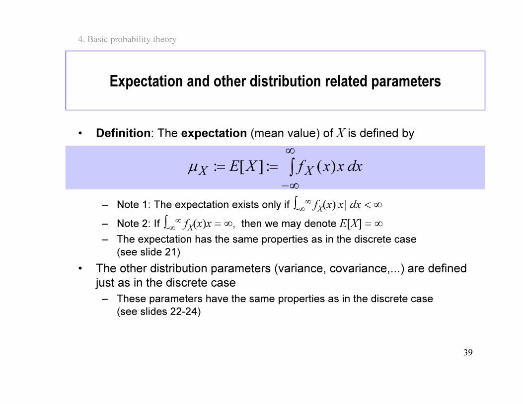
Expectation and other distribution related parameters
• Definition: The expectation (mean value) of X is defined by
– Note 1: The expectation exists only if ∫-∞
∞ fX(x)|x| dx < ∞
– Note 2: If ∫-∞
∞ fX(x)x = ∞, then we may denote E[X] = ∞
– The expectation has the same properties as in the discrete case
(see slide 21)
• The other distribution parameters (variance, covariance,...) are defined
just as in the discrete case
– These parameters have the same properties as in the discrete case
(see slides 22-24)
∫∞
∞−
== dxxxfXE XX )(:][:µ
40
4. Basic probability theory
Contents
• Basic concepts
• Discrete random variables
• Discrete distributions (nbr distributions)
• Continuous random variables
• Continuous distributions (time distributions)
• Other random variables
41
4. Basic probability theory
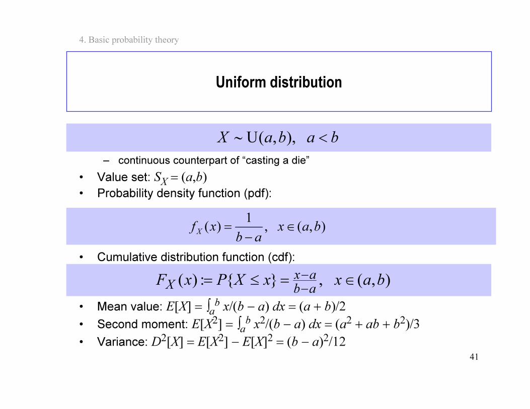
Uniform distribution
– continuous counterpart of “casting a die”
• Value set: SX= (a,b)
• Probability density function (pdf):
• Cumulative distribution function (cdf):
• Mean value: E[X] = ∫ab x/(b − a) dx = (a + b)/2
• Second moment: E[X2] = ∫ab x2/(b − a) dx = (a2 + ab + b2)/3
• Variance: D2[X] = E[X2] − E[X]2 = (b − a)2/12
babaX <∼ ),,(U
),( ,1
)( baxab
xfX
∈
−
=
),( ,:)( baxxXPxFab
axX ∈=≤=
−
−
42
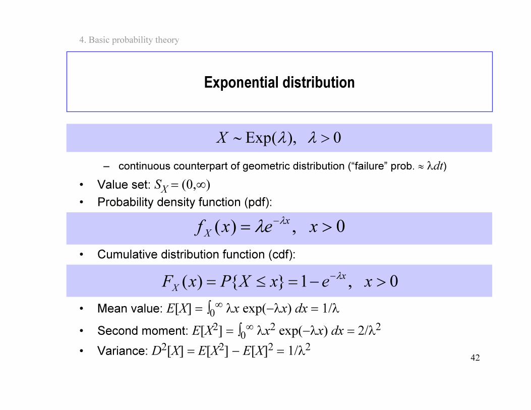
4. Basic probability theory
Exponential distribution
– continuous counterpart of geometric distribution (“failure” prob. ≈ λdt)
• Value set: SX= (0,∞)
• Probability density function (pdf):
• Cumulative distribution function (cdf):
• Mean value: E[X] = ∫0∞ λx exp(−λx) dx = 1/λ
• Second moment: E[X2] = ∫0∞ λx2 exp(−λx) dx = 2/λ2
• Variance: D2[X] = E[X2] − E[X]2 = 1/λ2
0 ),(Exp >∼ λλX
0 ,)( >=− xexf x
X
λλ
0 ,1)( >−=≤=−
xexXPxFx
X
λ
43
4. Basic probability theory
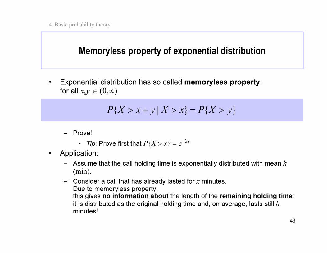
Memoryless property of exponential distribution
• Exponential distribution has so called memoryless property:
for all x,y ∈ (0,∞)
– Prove!
• Tip: Prove first that PX > x = e−λx
• Application:
– Assume that the call holding time is exponentially distributed with mean h (min).
– Consider a call that has already lasted for x minutes. Due to memoryless property, this gives no information about the length of the remaining holding time:
it is distributed as the original holding time and, on average, lasts still h minutes!
| yXPxXyxXP >=>+>
44
4. Basic probability theory
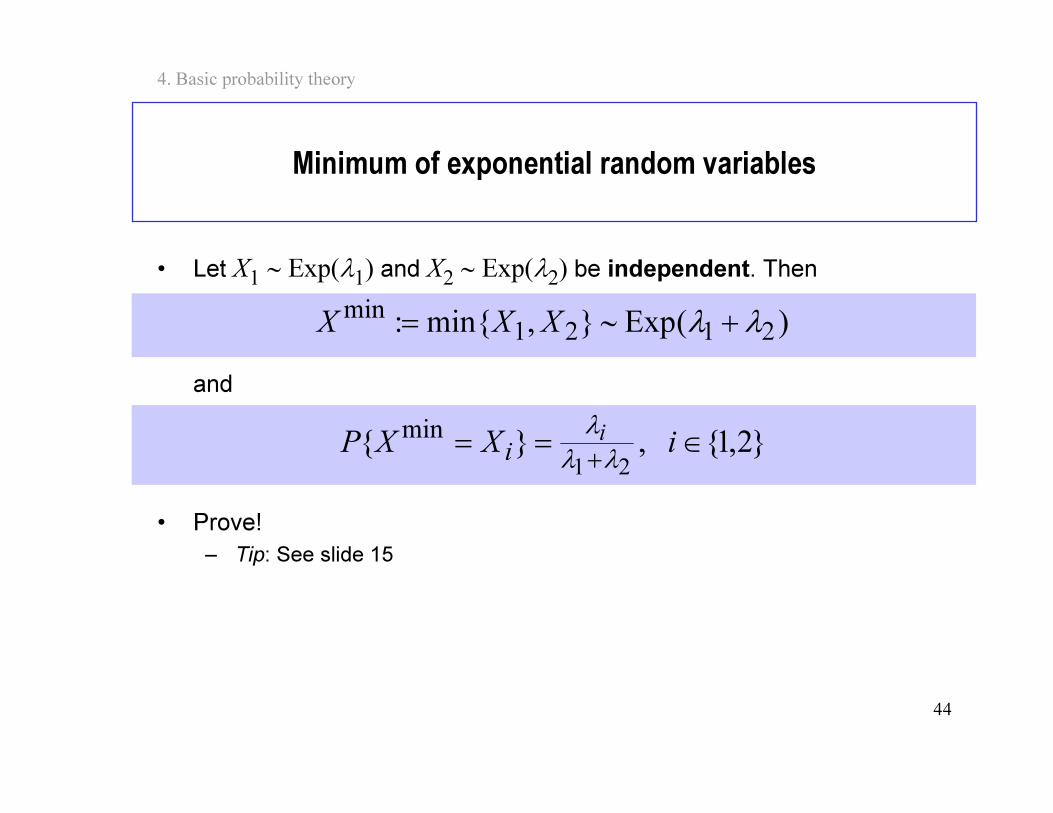
Minimum of exponential random variables
• Let X1∼ Exp(λ
1) and X
2∼ Exp(λ
2) be independent. Then
and
• Prove!
– Tip: See slide 15
)(Exp,min: 2121min
λλ +∼= XXX
2,1 ,21
min∈==
+iXXP
i
i λλ
λ
45
4. Basic probability theory
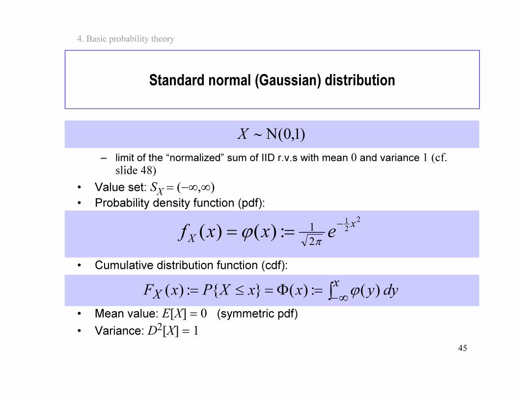
Standard normal (Gaussian) distribution
– limit of the “normalized” sum of IID r.v.s with mean 0 and variance 1 (cf. slide 48)
• Value set: SX= (−∞,∞)
• Probability density function (pdf):
• Cumulative distribution function (cdf):
• Mean value: E[X] = 0 (symmetric pdf)
• Variance: D2[X] = 1
)1,0(N∼X
2
2
1
2
1:)()(x
Xexxf−
==π
ϕ
∫∞−
=Φ=≤=x
X dyyxxXPxF )(:)(:)( ϕ
46
4. Basic probability theory
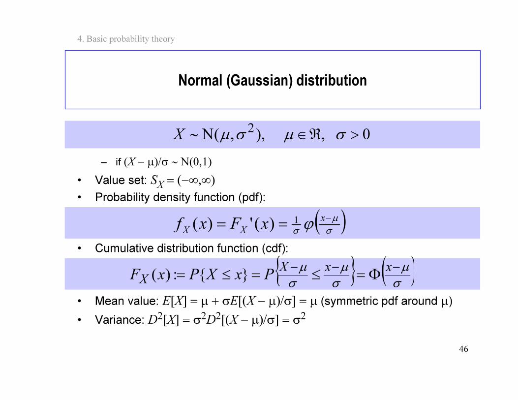
Normal (Gaussian) distribution
– if (X − µ)/σ ∼ N(0,1)
• Value set: SX= (−∞,∞)
• Probability density function (pdf):
• Cumulative distribution function (cdf):
• Mean value: E[X] = µ + σE[(X − µ)/σ] = µ (symmetric pdf around µ)
• Variance: D2[X] = σ2D2[(X − µ)/σ] = σ2
0 , ),,(N 2>ℜ∈∼ σµσµX
( )σ
µ
σϕ
−
==
x
XXxFxf 1)(')(
( )σ
µ
σ
µ
σ
µ −−−
Φ=≤=≤=xxX
X PxXPxF :)(
47
4. Basic probability theory
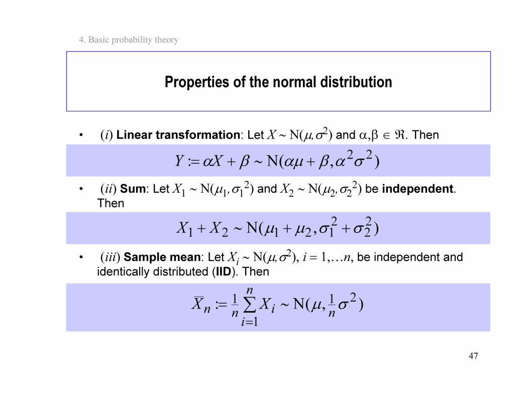
Properties of the normal distribution
• (i) Linear transformation: Let X ∼ N(µ,σ2) and α,β ∈ ℜ. Then
• (ii) Sum: Let X1∼ N(µ
1,σ
12) and X
2∼ N(µ
2,σ
22) be independent.
Then
• (iii) Sample mean: Let Xi∼ N(µ,σ2), i = 1,…n, be independent and
identically distributed (IID). Then
),(N: 22σαβαµβα +∼+= XY
),(N 22
212121 σσµµ ++∼+ XX
),(N: 21
1
1σµ
n
n
i
inn XX ∼= ∑=
48
4. Basic probability theory
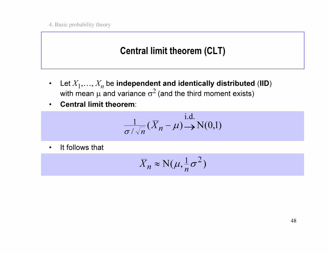
Central limit theorem (CLT)
• Let X1,…, X
nbe independent and identically distributed (IID)
with mean µ and variance σ2 (and the third moment exists)• Central limit theorem:
• It follows that
)1,0(N)(i.d.
/
1→− µ
σn
n
X
),(N 21σµ
nn
X ≈
49
4. Basic probability theory
Contents
• Basic concepts
• Discrete random variables
• Discrete distributions (nbr distributions)
• Continuous random variables
• Continuous distributions (time distributions)
• Other random variables
50
4. Basic probability theory
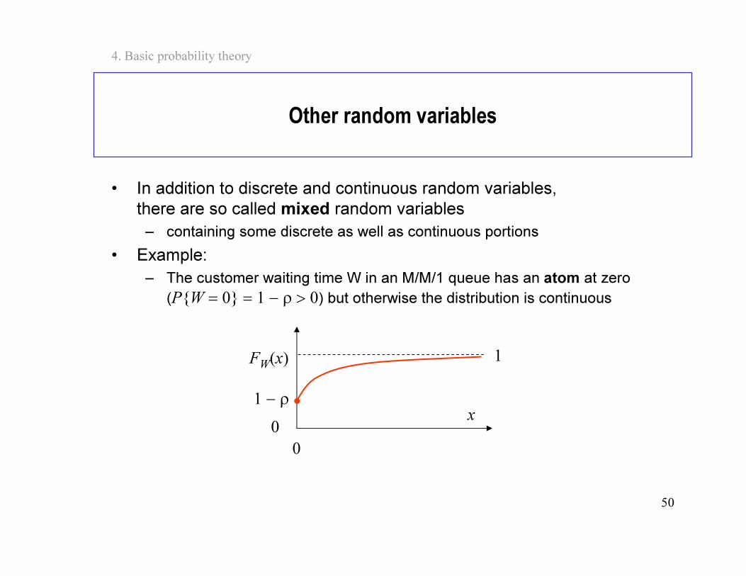
Other random variables
• In addition to discrete and continuous random variables,
there are so called mixed random variables
– containing some discrete as well as continuous portions
• Example:
– The customer waiting time W in an M/M/1 queue has an atom at zero
(PW = 0 = 1 − ρ > 0) but otherwise the distribution is continuous
FW(x)
x0
1
0
1 − ρ