AMS 212B Perturbation Methods - University of California...
12
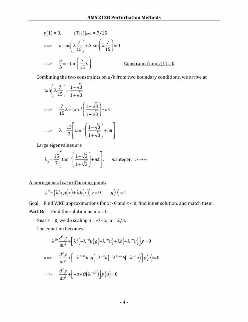
- 1 - AMS 212B Perturbation Methods Lecture 14 Copyright by Hongyun Wang, UCSC Example: Eigenvalue problem with a turning point inside the interval ′′ y + λ 2 x 1 − x 2 ⎛ ⎝ ⎜ ⎞ ⎠ ⎟ 2 y = 0 y −1 ( ) = 0, y 1 () = 0 ⎧ ⎨ ⎪ ⎪ ⎩ ⎪ ⎪ The ODE for y(x) has the form y’’(x)+λ 2 f(x) y(x) = 0 with f(x)= x(1-x/2) 2 . The WKB expansion for x > 0 and x < 0: φ 0 x ( ) =±i fs () ds 0 x ∫ =±i s 1 − s 2 ⎛ ⎝ ⎜ ⎞ ⎠ ⎟ ds 0 x ∫ =±i 2 3 x 3 2 − 1 5 x 5 2 ⎛ ⎝ ⎜ ⎞ ⎠ ⎟ = ±iT 1+ , x > 0 ±T 1− , x < 0 ⎧ ⎨ ⎪ ⎩ ⎪ where T 1+ = 2 3 x 3 2 − 1 5 x 5 2 ⎛ ⎝ ⎜ ⎞ ⎠ ⎟ , x > 0 T 1− = 2 3 x 3 2 + 1 5 x 5 2 ⎛ ⎝ ⎜ ⎞ ⎠ ⎟ , x < 0 φ 1 x ( ) = − 1 4 log f x ( ) = − 1 4 log x 1 − x 2 ⎛ ⎝ ⎜ ⎞ ⎠ ⎟ 2 A general solution at large λ is yx ( ) = 1 x 1 − x /2 ( ) 2 1/4 a ⋅ cos λT 1+ ( ) + b ⋅ sin λT 1+ ( ) ⎡ ⎣ ⎤ ⎦ , x > 0 1 x 1 − x /2 ( ) 2 1/4 c ⋅ exp λT 1− ( ) + d ⋅ exp −λT 1− ( ) ⎡ ⎣ ⎤ ⎦ , x < 0 ⎧ ⎨ ⎪ ⎪ ⎪ ⎪ ⎩ ⎪ ⎪ ⎪ ⎪ Suppose y(t) is the eigenfunction of a large eigenvalue λ. y(-1) = 0 (T1–)|x=–1 = 13/15
Transcript of AMS 212B Perturbation Methods - University of California...
- 1 -
AMS212BPerturbationMethodsLecture14
CopyrightbyHongyunWang,UCSC
Example:
Eigenvalueproblemwithaturningpointinsidetheinterval
′′y +λ2x 1− x2⎛⎝⎜
⎞⎠⎟
2
y =0
y −1( ) =0 , y 1( ) =0
⎧
⎨⎪⎪
⎩⎪⎪
TheODEfory(x)hastheformy’’(x)+λ2f(x)y(x)=0withf(x)=x(1-x/2)2.
TheWKBexpansionforx>0andx<0:
φ0 x( ) = ±i f s( )ds
0
x
∫ = ±i s 1− s2⎛⎝⎜
⎞⎠⎟ds
0
x
∫ = ±i 23 x32 − 15 x
52
⎛
⎝⎜⎞
⎠⎟=
±iT1+ , x >0±T1− , x <0
⎧⎨⎪
⎩⎪
where
T1+ =23 x
32 − 15 x
52
⎛
⎝⎜⎞
⎠⎟, x >0
T1− =23 x
32 + 15 x
52
⎛
⎝⎜⎞
⎠⎟, x <0
φ1 x( ) = −14 log f x( ) = −14 log x 1− x2
⎛⎝⎜
⎞⎠⎟
2
Ageneralsolutionatlargeλis
y x( ) =
1
x 1− x /2( )21/4 a⋅cos λT1+( )+b ⋅sin λT1+( )⎡⎣ ⎤⎦ , x >0
1
x 1− x /2( )21/4 c ⋅exp λT1−( )+d ⋅exp −λT1−( )⎡⎣ ⎤⎦ , x <0
⎧
⎨
⎪⎪⎪⎪
⎩
⎪⎪⎪⎪
Supposey(t)istheeigenfunctionofalargeeigenvalueλ.
y(-1)=0 (T1–)|x=–1=13/15
AMS212BPerturbationMethods
- 2 -
==>c ⋅exp λ1315
⎛⎝⎜
⎞⎠⎟+d ⋅exp −λ1315
⎛⎝⎜
⎞⎠⎟=0
==>cd= −exp −λ2615
⎛⎝⎜
⎞⎠⎟≈0
Usingtheconnectionformulas,wehave
a= 122d + c( )
b= 122d − c( )
⎧
⎨⎪⎪
⎩⎪⎪
==>ab= 2+ c /d2− c /d ≈1 Constraintfromy(-1)=0
Ontheotherhand,usingtheboundaryconditionatx=1,weobtain
y(1)=0, (T1+)|x=1=7/15
==>a⋅cos λ 715
⎛⎝⎜
⎞⎠⎟+b ⋅sin λ 715
⎛⎝⎜
⎞⎠⎟=0
==>ab= − tan λ 715
⎛⎝⎜
⎞⎠⎟ Constraintfromy(1)=0
Combiningthetwoconstraintsona/bfromtwoboundaryconditions,wearriveat
tan λ 715
⎛⎝⎜
⎞⎠⎟= −1 ==> λ(7/15)=(n–1/4)π
==> λ=(15/7)(n–1/4)π
Largeeigenvaluesare
λn ≈
157 n− 14⎛⎝⎜
⎞⎠⎟π , n=integer,nlarge.
Nextweconsiderthecasewhereoneboundaryconditionfallsontheturningpoint.
Example (Skipthisexampleinlecture):
Eigenvalueproblemwithaturningpointataboundary
AMS212BPerturbationMethods
- 3 -
′′y +λ2x 1− x2⎛⎝⎜
⎞⎠⎟
2
y =0
y 0( ) =0 , y 1( ) =0
⎧
⎨⎪⎪
⎩⎪⎪
TheWKBexpansionforx>0:
y WKB( ) x( ) = 1
x 1− x /2( )21/4 a⋅cos λT1+( )+b ⋅sin λT1+( )⎡⎣ ⎤⎦ , x >0
whereT1+ =
23 x
32 − 15 x
52
⎛
⎝⎜⎞
⎠⎟
Theinnersolutionnearx=0:
yinn( ) x( ) =αAi −λ
23x( )+βBi −λ2
3x( ) Atx=0,wehave
y(0)=0 ==> αAi(0)+βBi(0)=0PropertyofAiryfunctions:
Ai 0( ) = Bi 0( )
3= 132/3Γ 2/3( ) ≠0
(Wewillderivethispropertywhenwediscussasymptoticexpansionsofintegrals).UsingthispropertyofAiryfunction,wehave
αβ= −
Bi 0( )Ai 0( )= − 3
Recalltherelationbetween(α,β)and(a,b)
a= 1π λ1/6
α+β
2⎛⎝⎜
⎞⎠⎟
b= 1π λ1/6
α−β
2⎛⎝⎜
⎞⎠⎟
⎧
⎨
⎪⎪
⎩
⎪⎪
==>ab= α+βα−β
= α /β+1α /β−1 =
− 3+1− 3−1
Constraintfromy(0)=0
Ontheotherhand,usingtheboundaryconditionatx=1,weobtain
AMS212BPerturbationMethods
- 4 -
y(1)=0, (T1+)|x=1=7/15
==>a⋅cos λ 715
⎛⎝⎜
⎞⎠⎟+b ⋅sin λ 715
⎛⎝⎜
⎞⎠⎟=0
==>ab= − tan 7
15λ⎛⎝⎜
⎞⎠⎟ Constraintfromy(1)=0
Combiningthetwoconstraintsona/bfromtwoboundaryconditions,wearriveat
tan λ 715
⎛⎝⎜
⎞⎠⎟= 1− 31+ 3
==>
715λ = tan
−1 1− 31+ 3
⎛
⎝⎜
⎞
⎠⎟ +nπ
==>λ = 157 tan−1 1− 3
1+ 3⎛
⎝⎜
⎞
⎠⎟ +nπ
⎡
⎣⎢⎢
⎤
⎦⎥⎥
Largeeigenvaluesare
λn ≈
157 tan−1 1− 3
1+ 3⎛
⎝⎜
⎞
⎠⎟ +nπ
⎡
⎣⎢⎢
⎤
⎦⎥⎥, n:integer, n→∞
Amoregeneralcaseofturningpoint:
′′y + λ2x g x( )+λh x( )( ) y =0 , g 0( ) =1 Goal: FindWKBapproximationsforx>0andx<0,findinnersolution,andmatchthem.
PartB: Findthesolutionnearx=0
Nearx=0,wedoscalingu=–λαx, α=2/3.
Theequationbecomes
λ2α d
2 ydu2
+ λ2 −λ−αu( )g −λ−αu( )+λh −λ−αu( )⎡⎣
⎤⎦ y =0
==>d2 ydu2
+ −λ2−3αu⋅ g −λ−αu( )+λ1−2αh −λ−αu( )⎡⎣
⎤⎦ y u( ) =0
==>d2 ydu2
+ −u+O λ−1/3( )⎡⎣
⎤⎦ y u( ) =0
AMS212BPerturbationMethods
- 5 -
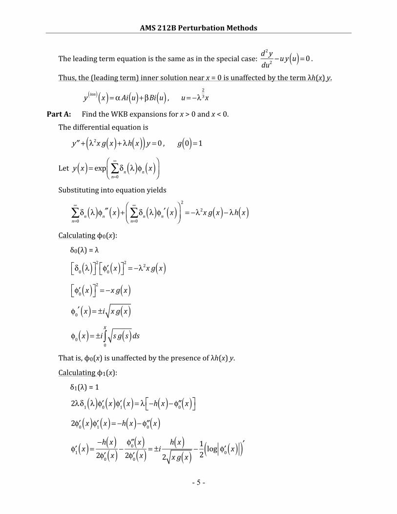
Theleadingtermequationisthesameasinthespecialcase:d2 ydu2
−u y u( ) =0 .Thus,the(leadingterm)innersolutionnearx=0isunaffectedbythetermλh(x)y.
yinn( ) x( ) =αAi u( )+βBi u( ) , u= −λ
23x
PartA: FindtheWKBexpansionsforx>0andx<0.
Thedifferentialequationis
′′y + λ2x g x( )+λh x( )( ) y =0 , g 0( ) =1
Lety x( ) = exp δn λ( )φn x( )
n=0
∞
∑⎛⎝⎜
⎞
⎠⎟
Substitutingintoequationyields
δn λ( )φn′′ x( )
n=0
∞
∑ + δn λ( )φn′ x( )n=0
∞
∑⎛⎝⎜
⎞
⎠⎟
2
= −λ2x g x( )−λh x( )
Calculatingϕ0(x):
δ0(λ)=λ
δ0 λ( )⎡⎣ ⎤⎦2
′φ0 x( )⎡⎣ ⎤⎦2= −λ2x g x( )
′φ0 x( )⎡⎣ ⎤⎦2= −x g x( )
φ0′ x( ) = ±i x g x( )
φ0 x( ) = ±i s g s( )ds
0
x
∫
Thatis,ϕ0(x)isunaffectedbythepresenceofλh(x)y.
Calculatingϕ1(x):
δ1(λ)=1
2λδ1 λ( ) ′φ0 x( ) ′φ1 x( ) = λ −h x( )− ′′φ0 x( )⎡⎣ ⎤⎦
2 ′φ0 x( ) ′φ1 x( ) = −h x( )− ′′φ0 x( )
′φ1 x( ) = −h x( )
2 ′φ0 x( ) −′′φ0 x( )
2 ′φ0 x( ) = ±ih x( )
2 x g x( )− 12 log ′φ0 x( )( )′
AMS212BPerturbationMethods
- 6 -
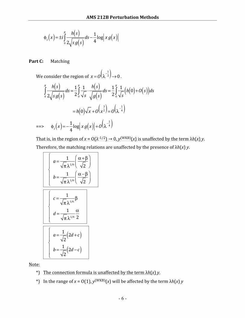
φ1 x( ) = ±i
h s( )2 s g s( )
ds0
x
∫ − 14 log x g x( )
PartC: Matching
Weconsidertheregionofx =O λ−12( )→0 .
h s( )2 s g s( )
ds0
x
∫ = 121s⋅h s( )g s( )
ds0
x
∫ = 121sh 0( )+O s( )( )ds
0
x
∫
= h 0( ) x +O x32( ) =O λ
−14( ) ==>
φ1 x( ) = −14 log x g x( ) +O λ
−14( ) Thatis,intheregionofx=O(λ-1/2)→0,y(WKB)(x)isunaffectedbythetermλh(x)y.
Therefore,thematchingrelationsareunaffectedbythepresenceofλh(x)y.
a= 1π λ1/6
α+β
2⎛⎝⎜
⎞⎠⎟
b= 1π λ1/6
α−β
2⎛⎝⎜
⎞⎠⎟
⎧
⎨
⎪⎪
⎩
⎪⎪
c = 1π λ1/6
β
d = 1π λ1/6
α2
⎧
⎨
⎪⎪
⎩
⎪⎪
a= 122d + c( )
b= 122d − c( )
⎧
⎨
⎪⎪
⎩
⎪⎪
Note: *) Theconnectionformulaisunaffectedbythetermλh(x)y.
*) Intherangeofx=O(1),y(WKB)(x)willbeaffectedbythetermλh(x)y
AMS212BPerturbationMethods
- 7 -
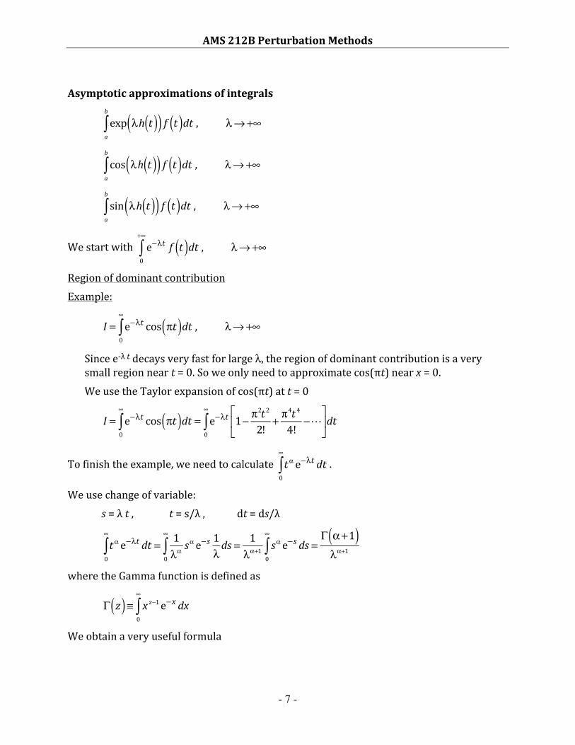
Asymptoticapproximationsofintegrals
exp λh t( )( ) f t( )dt
a
b
∫ , λ→ +∞
cos λh t( )( ) f t( )dt
a
b
∫ , λ→ +∞
sin λh t( )( ) f t( )dt
a
b
∫ , λ→ +∞
Westartwithe−λt f t( )dt
0
+∞
∫ , λ→ +∞
RegionofdominantcontributionExample:
I = e−λt cos πt( )dt
0
∞
∫ , λ→ +∞
Sincee-λtdecaysveryfastforlargeλ,theregionofdominantcontributionisaverysmallregionneart=0.Soweonlyneedtoapproximatecos(πt)nearx=0.WeusetheTaylorexpansionofcos(πt)att=0
I = e−λt cos πt( )dt
0
∞
∫ = e−λt 1− π2t2
2! + π4t 4
4! −!⎡
⎣⎢
⎤
⎦⎥dt
0
∞
∫
Tofinishtheexample,weneedtocalculatetα e−λt dt
0
∞
∫ .
Weusechangeofvariable: s=λt, t=s/λ, dt=ds/λ
tα e−λt dt
0
∞
∫ = 1λα s
α e−s 1λds
0
∞
∫ = 1λα+1 sα e−s ds
0
∞
∫ =Γ α+1( )λα+1
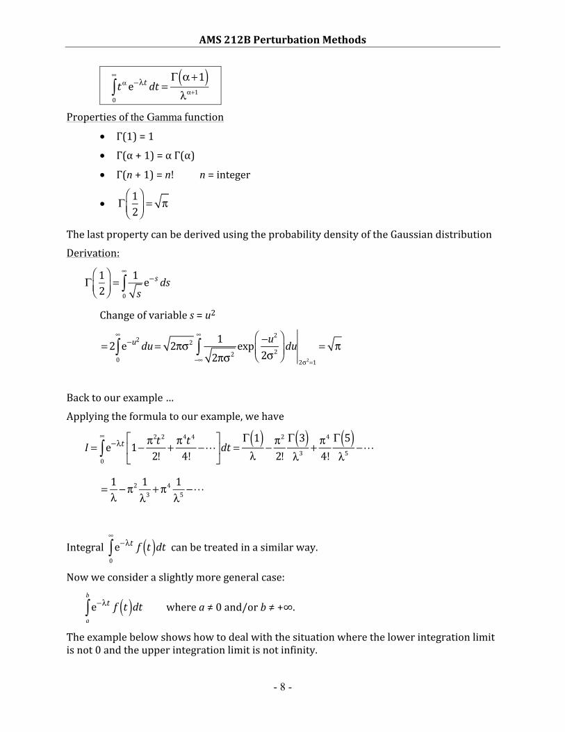
wheretheGammafunctionisdefinedas
Γ z( )≡ x z−1 e−x dx
0
∞
∫
Weobtainaveryusefulformula
AMS212BPerturbationMethods
- 8 -
tα e−λt dt
0
∞
∫ =Γ α+1( )λα+1
Propertiesofthe Gammafunction
• Γ(1)=1
• Γ(α+1)=αΓ(α)
• Γ(n+1)=n! n=integer
• Γ 12
⎛⎝⎜
⎞⎠⎟= π
ThelastpropertycanbederivedusingtheprobabilitydensityoftheGaussiandistribution
Derivation:
Γ 12
⎛⎝⎜
⎞⎠⎟= 1
se−s ds
0
∞
∫
Changeofvariables=u2
=2 e−u2du
0
∞
∫ = 2πσ2 12πσ2
exp −u2
2σ2⎛
⎝⎜⎞
⎠⎟du
−∞
∞
∫2σ2=1
= π
Backtoourexample…
Applyingtheformulatoourexample,wehave
I = e−λt 1− π2t2
2! + π4t 4
4! −!⎡
⎣⎢
⎤
⎦⎥dt
0
∞
∫ =Γ 1( )λ
− π2
2!Γ 3( )λ3
+ π4
4!Γ 5( )λ5
−!
= 1λ−π2 1
λ3+π4 1
λ5−!
Integrale−λt f t( )dt
0
∞
∫ canbetreatedinasimilarway.
Nowweconsideraslightlymoregeneralcase:
e−λt f t( )dt
a
b
∫ wherea≠0and/orb≠+∞.
Theexamplebelowshowshowtodealwiththesituationwherethelowerintegrationlimitisnot0andtheupperintegrationlimitisnotinfinity.
AMS212BPerturbationMethods
- 9 -
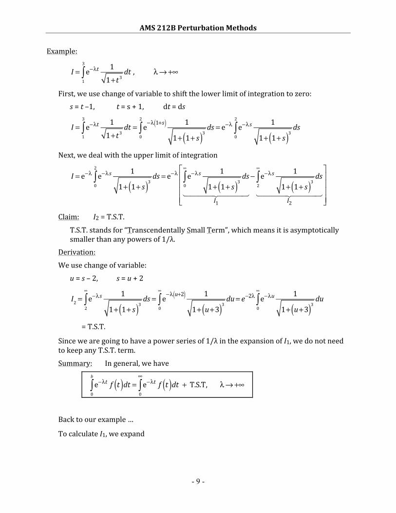
Example:
I = e−λt 1
1+t3dt
1
3
∫ , λ→ +∞
First,weusechangeofvariabletoshiftthelowerlimitofintegrationtozero: s=t–1, t=s+1, dt=ds
I = e−λt 1
1+t3dt
1
3
∫ = e−λ 1+s( ) 11+ 1+ s( )3
ds0
2
∫ = e−λ e−λs 11+ 1+ s( )3
ds0
2
∫
Next,wedealwiththeupperlimitofintegration
I = e−λ e−λs 11+ 1+ s( )3
ds0
2
∫ = e−λ e−λs 11+ 1+ s( )3
ds0
∞
∫
I1! "### $###
− e−λs 11+ 1+ s( )3
ds2
∞
∫
I2! "### $###
⎡
⎣
⎢⎢⎢⎢
⎤
⎦
⎥⎥⎥⎥
Claim: I2=T.S.T.
T.S.T.standsfor“TranscendentallySmallTerm”,whichmeansitisasymptoticallysmallerthananypowersof1/λ.
Derivation:
Weusechangeofvariable:
u=s–2, s=u+2
I2 = e−λs 1
1+ 1+ s( )3ds
2
∞
∫ = e−λ u+2( ) 11+ u+3( )3
du0
∞
∫ = e−2λ e−λu 11+ u+3( )3
du0
∞
∫
=T.S.T.
Sincewearegoingtohaveapowerseriesof1/λintheexpansionofI1,wedonotneedtokeepanyT.S.T.term.
Summary: Ingeneral,wehave
e−λt f t( )dt
0
b
∫ = e−λt f t( )dt0
∞
∫ + T.S.T, λ→ +∞
Backtoourexample…
TocalculateI1,weexpand
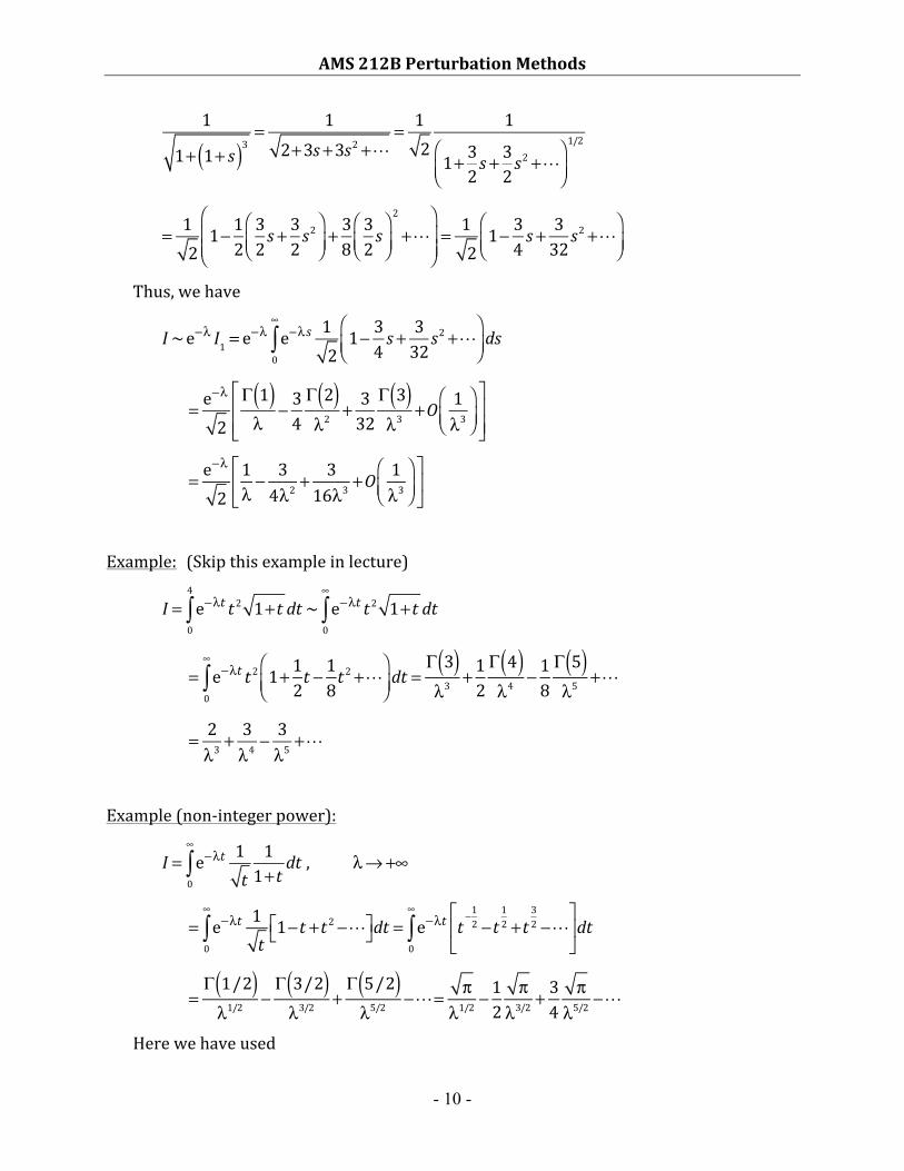
AMS212BPerturbationMethods
- 10 -
11+ 1+ s( )3
= 12+3s +3s2 +!
= 12
1
1+ 32 s +32 s
2 +!⎛⎝⎜
⎞⎠⎟
1/2
= 1
21− 12
32 s +
32 s
2⎛⎝⎜
⎞⎠⎟+ 38
32 s
⎛⎝⎜
⎞⎠⎟
2
+!⎛
⎝⎜⎜
⎞
⎠⎟⎟= 1
21− 34 s +
332 s
2 +!⎛⎝⎜
⎞⎠⎟
Thus,wehave
I~e−λ I1 = e−λ e−λs 1
21− 34 s +
332 s
2 +!⎛⎝⎜
⎞⎠⎟ds
0
∞
∫
= e
−λ
2Γ 1( )λ
− 34Γ 2( )λ2
+ 332
Γ 3( )λ3
+O 1λ3
⎛⎝⎜
⎞⎠⎟
⎡
⎣⎢⎢
⎤
⎦⎥⎥
= e
−λ
21λ− 34λ2 +
316λ3 +O
1λ3
⎛⎝⎜
⎞⎠⎟
⎡
⎣⎢
⎤
⎦⎥
Example: (Skipthisexampleinlecture)
I = e−λt t2 1+t dt
0
4
∫ ~ e−λt t2 1+t dt0
∞
∫
= e−λt t2 1+ 12t −
18t
2 +!⎛⎝⎜
⎞⎠⎟dt
0
∞
∫ =Γ 3( )λ3
+ 12Γ 4( )λ4
− 18Γ 5( )λ5
+!
= 2λ3
+ 3λ4
− 3λ5
+!
Example(non-integerpower):
I = e−λt 1
t11+t dt0
∞
∫ , λ→ +∞
= e−λt 1
t1−t +t2 −!⎡⎣ ⎤⎦dt
0
∞
∫ = e−λt t −12 −t
12 +t
32 −!
⎡
⎣⎢
⎤
⎦⎥dt
0
∞
∫
=Γ 1/2( )λ1/2
−Γ 3/2( )λ3/2
+Γ 5/2( )λ5/2
−!= πλ1/2
− 12π
λ3/2+ 34
πλ5/2
−!
Herewehaveused
AMS212BPerturbationMethods
- 11 -
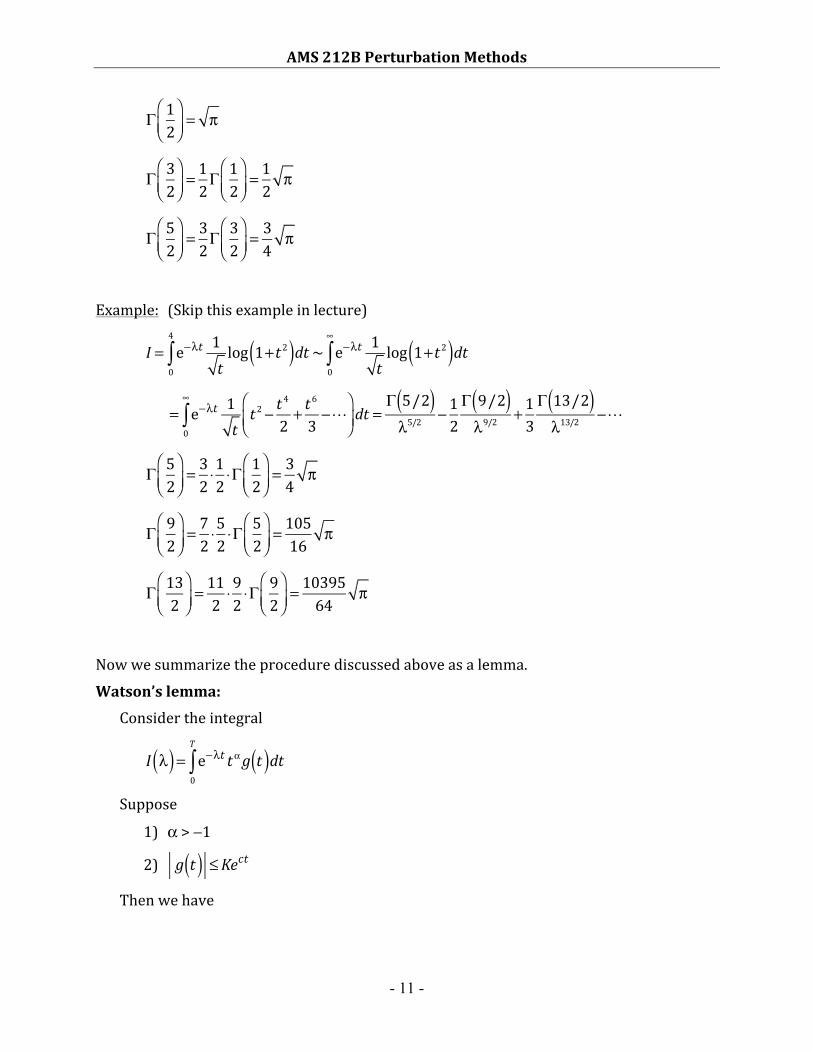
Γ 12
⎛⎝⎜
⎞⎠⎟= π
Γ 32
⎛⎝⎜
⎞⎠⎟= 12Γ
12
⎛⎝⎜
⎞⎠⎟= 12 π
Γ 52
⎛⎝⎜
⎞⎠⎟= 32Γ
32
⎛⎝⎜
⎞⎠⎟= 34 π
Example: (Skipthisexampleinlecture)
I = e−λt 1
tlog 1+t2( )dt
0
4
∫ ~ e−λt 1tlog 1+t2( )dt
0
∞
∫
= e−λt 1
tt2 − t
4
2 + t6
3 −!⎛
⎝⎜⎞
⎠⎟dt
0
∞
∫ =Γ 5/2( )λ5/2
− 12Γ 9/2( )λ9/2
+ 13Γ 13/2( )λ13/2
−!
Γ 52
⎛⎝⎜
⎞⎠⎟= 32 ⋅
12 ⋅Γ
12
⎛⎝⎜
⎞⎠⎟= 34 π
Γ 92
⎛⎝⎜
⎞⎠⎟= 72 ⋅
52 ⋅Γ
52
⎛⎝⎜
⎞⎠⎟= 10516 π
Γ 13
2⎛⎝⎜
⎞⎠⎟= 112 ⋅92 ⋅Γ
92
⎛⎝⎜
⎞⎠⎟= 1039564 π
Nowwesummarizetheprocedurediscussedaboveasalemma.
Watson’slemma:Considertheintegral
I λ( ) = e−λt tαg t( )dt
0
T
∫
Suppose
1) α>−1
2)g t( ) ≤Kect
Thenwehave
AMS212BPerturbationMethods
- 12 -
I λ( )~ g n( ) 0( )
n!Γ α+n+1( )
λα+n+1n=0
N
∑
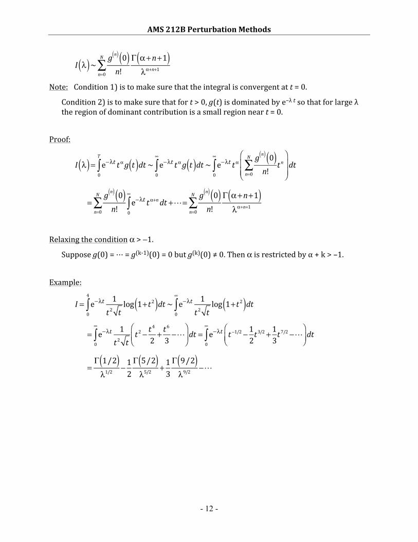
Note: Condition1)istomakesurethattheintegralisconvergentatt=0.
Condition2)istomakesurethatfort>0,g(t)isdominatedbye–λtsothatforlargeλtheregionofdominantcontributionisasmallregionneart=0.
Proof:
I λ( ) = e−λt tαg t( )dt
0
T
∫ ~ e−λt tαg t( )dt0
∞
∫ ~ e−λt tαg n( ) 0( )n! t n
n=0
N
∑⎛
⎝⎜⎜
⎞
⎠⎟⎟dt
0
∞
∫
=
g n( ) 0( )n! e−λt tα+n dt
0
∞
∫n=0
N
∑ +!=g n( ) 0( )n!
Γ α+n+1( )λα+n+1
n=0
N
∑
Relaxingtheconditionα>−1.
Supposeg(0)=⋯=g(k-1)(0)=0butg(k)(0)≠0.Thenαisrestrictedbyα+k>–1.
Example:
I = e−λt 1
t2 tlog 1+t2( )dt
0
4
∫ ~ e−λt 1t2 t
log 1+t2( )dt0
∞
∫
= e−λt 1
t2 tt2 − t
4
2 + t6
3 −!⎛
⎝⎜⎞
⎠⎟dt
0
∞
∫ = e−λt t −1/2 − 12t3/2 + 13t
7/2 −!⎛⎝⎜
⎞⎠⎟dt
0
∞
∫
=Γ 1/2( )λ1/2
− 12Γ 5/2( )λ5/2
+ 13Γ 9/2( )λ9/2
−!