Aggregation of α-synuclein monomers and engineered ... · CHAPTER 1: INTRODUCTION AND ... (3D)...
141
Aggregation of α-synuclein monomers and engineered oligomers in solution by Xi Li A thesis submitted in partial fulfillment of the requirements for the degree of Master of Science Department of Chemistry University of Alberta © Xi Li, 2015
Transcript of Aggregation of α-synuclein monomers and engineered ... · CHAPTER 1: INTRODUCTION AND ... (3D)...
Aggregation of α-synuclein monomers and
engineered oligomers in solution
by
Xi Li
A thesis submitted in partial fulfillment of the requirements for the degree of
Master of Science
Department of Chemistry
University of Alberta
© Xi Li, 2015
ii
Abstract
α-Synuclein is a protein that has been found as fibrillar aggregates in Lewy bodies
in the brain of Parkinson’s disease patients. Though the cause of the Parkinson’s
disease is unknown, previous research suggest that there is a close association
between the disease and the toxicity of the intermediary α-synuclein oligomers in
human neurons. Therefore, it is important to investigate the aggregation behaviour
of intermediary oligomers. To do this we investigate aggregation of protein
constructs that are monomers (Snca1), or engineered dimers (Snca2), tetramers
(Snca4), and octamers (Snca8) of α-synuclein with a C terminal cysteine. Single-
molecule fluorescence methods were used to study the molecular interactions
between pairs of these oligomers under “physiological” aggregation conditions
(10 mM PBS at pH = 7.4 at 37 °C). To be specific, we applied dual-color
fluorescence cross correlation spectroscopy (dual-color FCCS) to study the self-
aggregation (aggregation of one kind of α-synuclein) and the cross-aggregation
(aggregation between the monomeric and oligomeric α-synuclein) of α-synuclein.
The engineered α-synuclein monomers, dimers, tetramers and octamers were
labelled with either Oregon Green 488 maleimide (green dye) or Cy5-tetrazine
(red dye). A green dye labelled protein was incubated with a red dye labelled
protein at micromolar concentrations with continuous shaking at 250 rpm and
diluted aliquots of the aggregation mixture was measured by dual-color FCCS at
nanomolar concentrations after different incubation times. The experimental
results indicate that the engineered α-synuclein octamers aggregate faster and to a
greater extent than monomers and dimers, with the tetramers being intermediate.

iii
The engineered oligomers preferred to incorporate themselves rather than the
monomer into aggregates. Therefore, these oligomer constructs do not appear to
seed the aggregation of monomers.

iv
Acknowledgements
I would first like to express my gratitude to my supervisor, Prof. Nils Petersen for
his continuous encouragement, wise guidance and inspiration. Without his support,
I would have never finished my degree. Throughout the two and half years in the
lab, I have learned invaluable lessons from Dr. Petersen on how to be professional,
positive, curious and passionate about research and life in general. I would also
like to thank the project leader, Prof. Michael Woodside, for giving me the
opportunity to work on this project in his lab and for continuously providing
beneficial feedback. Then, I would like to thank Prof. Charles Lucy and Prof.
Julianne Gibbs-Davis for offering me great insights for my career and into my
research.
There are many exceptional colleagues that have to be thanked for helping me
through this stage of my life, they are Meijing Wang, Lindsay Shearer, Chunhua
Dong, Nick Smisdom, Daniel Foster, Derek Dee, Craig Garen, Supratik Sen
Mojumdar, Marion Becker, Armin Hoffmann, Allison Solanki, Angela Brigley ....
I really appreciate that I had a chance to work with these professional, caring and
very interesting researchers to produce some high-quality results.
In the end, my deepest thanks and love are given to my grandparents, my parents,
my cousins, and my partner, Lei, who have been of great support and motivation
for me throughout these years. Without them, I would never make it this far in my
studies. I am so thankful and blessed to have them in my life.
v
TABLE OF CONTENTS
ABSTRACT .......................................................................................................... II
ACKNOWLEDGEMENTS ............................................................................... IV
LIST OF FIGURES ......................................................................................... VIII
LIST OF TABLES ........................................................................................... XIII
LIST OF SYMBOLS, NOMENCLATURE OR ABBREVIATIONS ........... XV
CHAPTER 1: INTRODUCTION AND LITERATURE REVIEW ................. 1
1.1 OVERVIEW OF NEURODEGENERATIVE DISEASES ............................................. 1
1.2 STUDIES OF THE AGGREGATION-PRONE PROTEINS .......................................... 4
1.2.1 Protein sequence alignment and comparison ......................................... 4
1.2.2 Protein hydrodynamic size measurement .............................................. 5
1.2.3 Protein three-dimensional (3D) structure estimation ............................. 5
1.2.4 Monitoring protein aggregation in vitro and in vivo ............................. 7
1.3 α-SYNUCLEIN ................................................................................................. 8
1.3.1 Research about α-synucleins (1997-2008) ............................................. 8
1.3.2 Recent research into α-synuclein (2009-2014) .................................... 12
1.4 MY RESEARCH OBJECTIVES .......................................................................... 15
CHAPTER 2: METHODOLOGY AND THEORY ......................................... 17
2.1 TECHNIQUES USED IN PROTEIN AGGREGATION STUDIES ............................... 17
2.1.1 Sodium dodecyl sulfate-polyacrylamide gel electrophoresis (SDS-
PAGE ............................................................................................................ 17
2.1.2 Size-exclusion chromatography ........................................................... 18
2.1.3 Dynamic light scattering (DLS) ........................................................... 20
2.2 FLUORESCENCE SPECTROSCOPY ................................................................... 22
2.2.1 Structure of a fluorescence microscope ............................................... 22
2.2.2 Fluorescence correlation spectroscopy (FCS) ..................................... 24
vi
The principle of FCS ................................................................................. 25
Physical meaning of the important parameters in FCS ............................. 27
Two-component FCS fitting equation ...................................................... 29
Other fitting factors needed to be considered ........................................... 30
2.2.3 Dual-color fluorescence cross-correlation spectroscopy (FCCS) ........ 32
The principle of dual-color FCCS ............................................................. 32
Other general factors need to be considered ............................................. 35
CHAPTER 3: MATERIALS AND METHODS .............................................. 38
3.1 LABELLING ................................................................................................... 38
3.2 PURIFICATION AND LABELLING EFFICIENCY ................................................. 44
3.2.1 Fast protein liquid chromatography (FPLC) ........................................ 44
3.2.1 Centrions, centrifuge, and UV/Vis spectroscopy ................................. 45
3.2.3 HPLC-ESI-oaTOF ............................................................................... 47
3.3 QUANTUM YIELDS OF LABELLED α-SYNUCLEINS .......................................... 49
3.4 DLS ............................................................................................................. 50
3.5 FCS AND DUAL-COLOR FCCS ...................................................................... 51
3.5.1 Calibration measurements .................................................................... 51
3.5.2 Hydrodynamic diameters of α-synucleins by FCS .............................. 67
3.5.3 Aggregation tests by FCS .................................................................... 67
3.5.4 Aggregation tests by dual-color FCCS. ............................................... 69
CHAPTER 4: RESULTS AND DISCUSSIONS .............................................. 74
4.1 PURIFICATION AND LABELLING EFFICIENCY ................................................. 74
4.1.1 Distinguishing non-specific binding from covalent labelling .............. 74
4.1.2 High labelling efficiency demonstrated by centrifugal purification .... 80
4.1.3 HPLC-MS confirms covalent labelling at high efficiency .................. 84
vii
4.1.4 HPLC-MS confirms coupling of TPM with α-synuclein ..................... 85
4.2 QUANTUM YIELDS OF OREGON GREEN 488 IS AFFECTED BY CONJUGATION TO
α-SYNUCLEINS.................................................................................................... 88
4.3 DETERMINATION OF HYDRODYNAMIC SIZE OF LABELLED Α-SYNUCLEINS .... 91
4.3.1 Hydrodynamic diameters of α-synucleins by DLS .............................. 91
4.3.2 Hydrodynamic diameters of α-synucleins by FCS .............................. 94
4.3.3 Hydrodynamic diameters of α-synucleins are independent of the
protein concentration. ................................................................................... 96
4.3.4 Overall Discussion ............................................................................... 97
4.4 AGGREGATION OF LABELLED α-SYNUCLEINS ............................................... 99
4.4.1 Aggregation tests by FCS .................................................................... 99
4.4.2 Aggregation tests by dual-color FCCS. ............................................. 101
CHAPTER 5: CONCLUSION ......................................................................... 113
5.1 RESEARCH SUMMARY AND CONTRIBUTIONS ............................................... 113
5.2 FUTURE WORKS .......................................................................................... 114
BIBLIOGRAPHY ............................................................................................. 115
viii
List of Figures
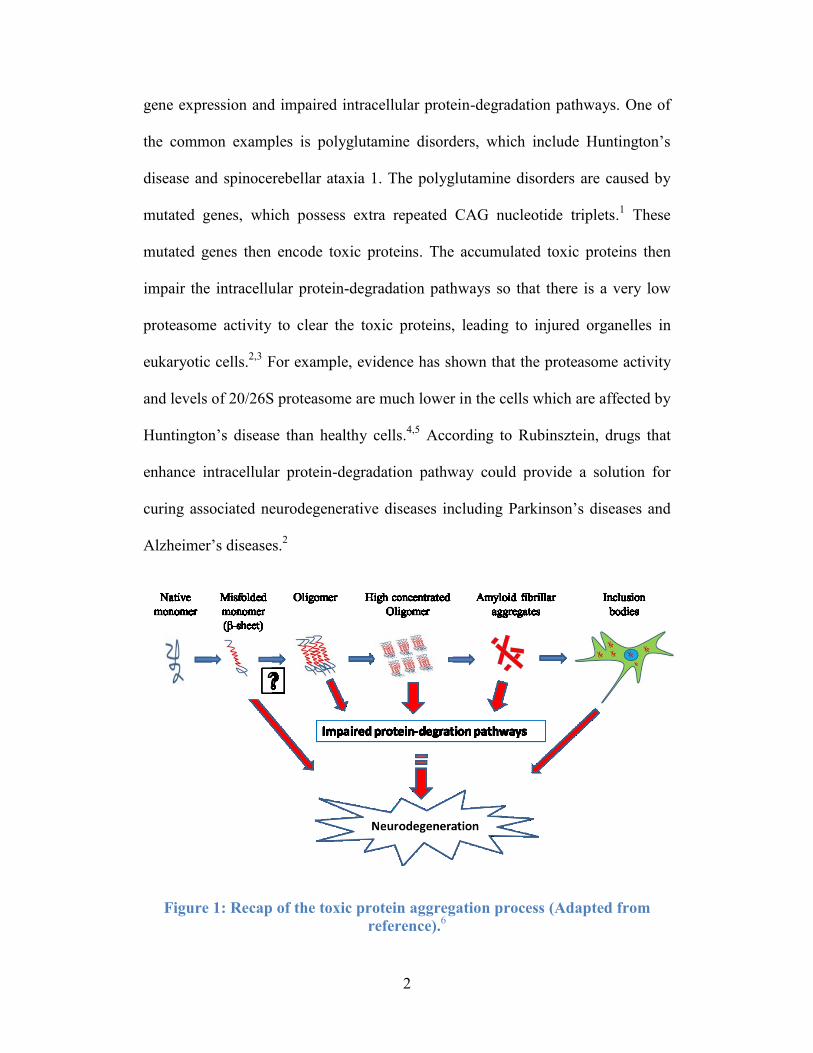
Figure 1: Recap of the toxic protein aggregation process (Adapted from
reference).6 .............................................................................................................. 2
Figure 2: Primary structure of α-synuclein labelled with seven KTKEGV motifs
and three mutation sites associated with familial Parkinson’s diseases (Adapted
from reference).68
.................................................................................................... 9
Figure 3: Formation of oligomers or fibrils with different morphology (Adapted
from reference).80
.................................................................................................. 11
Figure 4: Principle of SEC (Adapted from reference).97
...................................... 19
Figure 5: Principle of DLS. ................................................................................... 20
Figure 6: A simplified diagram of confocal microscope with two detectors. ....... 24
Figure 7: Principle of FCS (Adapted from reference).107
..................................... 26
Figure 8: (a) Autocorrelation function of two component translational
fluctuations; (b) Autocorrelation function for one component translational
fluctuation with triplet and rotational diffusion. ................................................... 31
Figure 9: Principle of dual-color FCCS. ............................................................... 33
Figure 10: Three common protein-dye labelling reactions. .................................. 41
Figure 11: Autocorrelation function and corresponding fitting curves (dashed
lines) of Cy5 excited by 488 nm (green) and 633 nm (red), respectively............. 52
ix
Figure 12: Autocorrelation functions and cross-correlation function of Rhodamine
6G. Red line is the fitting curve of data obtained by the red detector, Green line is
from the green detector, Black line is data calculated based on the cross
correlation function. .............................................................................................. 55
Figure 13: Count rate is a function of laser powers at different concentrations of
Alexa Fluor® 488 C5-maleimide. Black is at 1312 nM, Red is at 656 nM, Green
is at 328 nM, Purple is at 164 nM and Blue is at 82 nM. ..................................... 56
Figure 14: Observed number of fluorescent particles in a confocal volume, N, as a
function of the concentrations of Alexa Fluor 488. .............................................. 61
Figure 15: Viscosity of 10% ethanol as a function of temperature. ...................... 65
Figure 16: Scheme of the aggregation tests by using FCS. .................................. 68
Figure 17: Scheme of the aggregation tests using dual-color FCCS. ................... 69
Figure 18: Comparison of FPLC elution profiles for Alexa Fluor® 488 C5-
Maleimide and Snca1. (a) Alexa Fluor® 488 at pH 7.40, (b) Snca1 at pH 7.40, (c)
Non-reacted the dye and Snca 1 at pH 7.40, (d) Non-reacted dye and Snca 1 at pH
4.68 and (e) Snca1_alexa Fluor® 488 C5-Maleimide . ........................................ 75
Figure 19: Comparison of FPLC elution profiles for CFTM
488A Dye and α-
synuclein. (a) CFTM
488A Dye, and (b) Snca1 mixed with CFTM
488A Dye
without labelling reaction. .................................................................................... 76
Figure 20: Comparison of FPLC elution profiles for Oregon Green® 488
Carboxylic Acid Succinimidyl Ester, 6-isomer dye and α-synuclein. (a) Oregon
x
Green® 488 Carboxylic Acid Dye, (b) The mixture of Snca8 and the dye, and (c)
Snca8_ ORNH488. ............................................................................................... 77
Figure 21: Comparison of FPLC elution profiles for Oregon Green® 488
Maleimide and α-synuclein. (a) Snca4_ORM488 using sulfhydryl maleimide
labelling Method One. (b) Snca4_ORM488 using sulfhydryl maleimide labelling
Method Two. ......................................................................................................... 79
Figure 22: (a) Spectra of TCO-PEG3-Maleimides (TPM) (yellow), the first filtrate
volume (black) and the second filtrate volume (blue) from centrifugation of the
Snca4 labelled with large amounts of TPM. (b) Spectra of Snca4_TPM (green),
spectra of Cy5 tetrazine (red) and spectra of Snca4_TPM_Cy5 (purple). ............ 81
Figure 23: Spectra of Oregon Green 488 maleimide (green), Snca4 before
labelling (yellow) and 5 µL of Snca4_ORM488 diluted by 20 times (purple). .... 83
Figure 24: MS spectra for labelled and unlabelled monomeric α-synuclein. ....... 85
Figure 25: MS spectrum for Snca1_Cys_TPM. .................................................... 87
Figure 26: MS spectrum for Snca2_Cys_TPM. .................................................... 87
Figure 27: Fluoresence as a function of emission wavelengths for Cy5 tetrazine
(Blue) and the mixture of Snca1_Cys and Cy5 tetrazine (Red). Dashed line
indicated the starting point (656 nm) of all integrated emission........................... 88
Figure 28: Fluoresence as a function of emission wavelength for Oregon Green
488 maleimide (Blue) and the mixture of Snca1_Cys and the dye (Red)............. 89
xi
Figure 29: Intensity particle size distributions of Snca1, 2, 4 and 8_Cys_TCM. . 93
Figure 30: Weighted-volume particle size distributions of Snca1, 2, 4 and
8_Cys_TPM. ......................................................................................................... 93
Figure 31: Fitted correlograms of Snca1, 2, 4, and 8_Cys_TPM. ........................ 94
Figure 32: (a) Distribution of the diffusion time of Snca1_Cys_Dye with
Snca1_Cys at different incubation times. (b) Distribution of the diffusion time of
Snca4_Cys_Dye with Snca4_Cys at different incubation times. ........................ 100
Figure 33: Distribution of the diffusion time of Snca4_Cys_Dye incubated with
Snca1_Cys at different times. ............................................................................. 101
Figure 34: (a) Autocorrelation functions and cross-correlation function of a
mixture of Snca8_ORM488 and Snca8_Cy5 at t = 0 hour. (b) Autocorrelation
functions and cross-correlation function of a mixture of Snca8_ORM488 and
Snca8_Cy5 at t = 6 hours. Red dashed line is the fitting curve of data obtained by
the red detector, Green dashed line is from the green detector and Black dashed is
data calculated based on the cross correlation. ................................................... 103
Figure 35: (a) 𝐧𝐫𝐠𝐧𝐫 as a function of incubation time; (b) 𝐧𝐫𝐠𝐧𝐠as a function of
incubation time for FCCS 11 (red), FCCS 22 (black), FCCS 44 (blue) and FCCS
88 (purple). .......................................................................................................... 104
Figure 36: (a) 𝒏𝒓𝒈𝒏𝒓 as a function of incubation time for FCCS 12, 14 and 18;
(b) 𝒏𝒓𝒈𝒏𝒈 as a function of incubation time for for FCCS 12, 14 and 18; (c)
𝒏𝒓𝒈𝒏𝒓 as a function of incubation time for FCCS 21, 41 and 81; (d) 𝒏𝒓𝒈𝒏𝒈 as a
xii
function of incubation time for FCCS 21, 41 and 81. Black for sample contained
dimeric α-synuclein, blue for tetramers and purple for octamers. ...................... 107
Figure 37: (a) and (b) are 𝐧𝐫𝐠𝐧𝐫 as a function of incubation time for FCCS 88
with and without continuous shaking, respectively. (c) and (d) are 𝐧𝐫𝐠𝐧𝐠 as a
function of incubation time for FCCS 88 with and without continuous shaking,
respectively. ........................................................................................................ 112
xiii
List of Tables
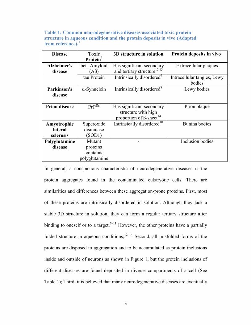
Table 1: Common neurodegenerative diseases associated toxic protein structure in
aqueous condition and the protein deposits in vivo. ............................................... 3
Table 2: The producer and name for each dye used in the research. .................... 39
Table 3: Selection of the Amicon® Ultra filters for Snca1, 2, 4 and 8. ................ 46
Table 4: The buffer gradient for α-synucleins. ..................................................... 48
Table 5: Molar absorptivities of Snca1, 2, 4 and 8. .............................................. 50
Table 6: G(0), N and τD of Rodamine 6G measured by FCCS. ........................... 54
Table 7: Count Rates of Oregon Green® 488 maleimide and Cy5 Tetrazine in
FCCS. .................................................................................................................... 57
Table 8: Fitting results of Oregon Green 488 maleimide in PBS at pH=7.40 in
FCS. ...................................................................................................................... 58
Table 9: Fitting results of Cy5 tetrazine in 10% of Ethanol in FCS. .................... 59
Table 10: Fitting results of Alexa Fluor® 488 C5-maleimide at different
concentration in PBS at pH=7.40 at 298.15 K in FCS. ......................................... 60
Table 11: t-Tests for comparing two independent values. .................................... 63
Table 12: Viscosity of 10% ethanol (by weight) at different temperature115
. ...... 64
Table 13: Viscosity of water, 10 mM PBS and 10% of Ethanol at 298.15 K. ...... 65
Table 14: Calculated diffusion coefficients (D) and diffusion times ( τD) of
different dyes in water, 10 mM PBS and 10% Ethanol at 298.15 K .................... 66
Table 15: Codes and repeated times of all dual-color FCCS experiments. .......... 70
Table 16: Expected mass and experimental result of Sncax_Cys_TPM. ............. 86
Table 17: Summary of relative quantum yields for Cy5 tetrazine alone, in mixture
with proteins and conjugated to proteins. ............................................................. 89
Table 18: Summary of relative quantum yields for Oregon Green 488 C5
maleimide alone, in mixture with proteins and conjugated to proteins. ............... 90
Table 19: Weighted-volume particle size distributions for α-synucleins. ............ 94
Table 20: Fitting results of labelled Snca1, 2, 4 and 8 in PBS at pH = 7.40 and
comparison of the hydrodynamic diameters obtained from FCS and DLS. ......... 95
xiv
Table 21: Fitting results of labelled Snca4 with different concentration of
unlabelled Snca4 in PBS at pH=7.40. ................................................................... 97
Table 22: Comparison of the estimated hydrodynamic diameters of Snca1, 2, 4,
and 8 with DLS and FCS results. .......................................................................... 98
Table 23: Summary of fitting amplitude of FCCS self-aggregation tests. ......... 105
Table 24: Summary of fitting amplitude of FCCS cross-aggregation tests. ....... 108
Table 25: Another format of summary the fitting amplitudes of all FCCS tests. 109
Table 26: Detailed information of fitting k values for all FCCS tests. ............... 111
xv
List of Symbols, Nomenclature or Abbreviations
Alexa 488 Alexa Fluor® 488 C5-maleimide
ATR-FTIR Attenuated total reflectance-Fourier transform infrared
Cy5 Cy5 Tetrazine
Cys Cysteine
DLS Dynamic light scattering
DMSO Dimethylsulfoxide
EM Electron microscopy
ESI Electrospray ionization
FCCS Fluorescence cross-correlation spectroscopy
FCS Fluorescence correlation spectroscopy
FPLC Fast protein liquid chromatography
FRET Forster resonance energy transfer
HFT Main dichroic beam splitter
HPLC-MS High performance liquid chromatography-mass spectrometry
ICS Image correlation spectroscopy
MS Mass spectrometry
NFT Secondary dichroic beam splitter
NMR Nuclear magnetic resonance
ORM488 Oregon Green® 488 maleimide
PBS Phosphate-buffered saline (137 mM NaCl, 2.7 mM KCl, 10 mM Na2HPO4
and 1.8 mM KH2PO4 )
SDS Sodium dodecyl sulfate
SH group Thiol group
smFS Single-molecule force spectroscopy
SDS-
PAGE Sodium dodecyl sulfate-polyacrylamide gel electrophoresis
TCEP-HCl Tris-(2-carboxyethyl) phosphine hydrochloride
TCO Trans-Cyclooctene group
TEM Transmission electron microscopy
ThT Thioflavin-T
TPM Trans-Cyclooctene-PEG3-Maleimide
A(… nm ) Absorbance at a specific wavelength
G(0) Amplitude of a correlation function of fluorescence fluctuation
Gg(0) Amplitude of a correlation function of green fluorescence fluctuation
Gr(0) Amplitude of a correlation function of red fluorescence fluctuation
Grg(0) Amplitude of a cross correlation function
Gg(τ) Autocorrelation function of green fluorescence fluctuation
Gr(τ) Autocorrelation function of red fluorescence fluctuation
⟨… ⟩ Average
NA Avogadro constant
k Boltzmann constant
c Concentration
CF Correction factor
G(τ) Correlation function
Grg(τ) Cross-correlation function
τD Diffusion time
xvi
τD1 Diffusion time of component 1
τD2 Diffusion time of component 2
τDrg Diffusion time of protein aggregates emitted green and red fluorescence
Veff Effective confocal volume
Veff_green Effective confocal volume of a green detector
Veff_red Effective confocal volume of a red detector
E Emission
wxy Equatorial radii of a confocal volume
wxy_green Equatorial radii of a confocal volume of a green detector
wxy_red Equatorial radii of a confocal volume of a red detector
ε(...) Molar absorptivity
δ Fluctuations around the mean
t1/2 Half time
R Hydrodynamic radius
Rrg Hydrodynamic radius of the aggregate emitted both green and red
fluorescence
F(t) Intensity of fluorescence intensity
I(t) Intensity of Rayleigh scattering
td Lag time
μ Mean
N Number of amino acids
N Observed number of fluorescent particles in a confocal volume
Ng Observed number of fluorescent particles in a green confocal
Nr Observed number of fluorescent particles in a red confocal volume
Nrg Observed number of fluorescent particles in a cross confocal volume
ng Observed number of fluorescent particles per unit green volume
nr Observed number of fluorescent particles per unit red volume
nrg Nrg divided by Veff_Cross
Veff_Cross Overlapped effective confocal volume of the green and red detector
wz Polar radii of the confocal volume
wz_green Polar radii of the confocal volume of a green detector
wz_red Polar radii of the confocal volume of a red detector
sm Standard error of the mean
T Temperature
D Translational diffusion coefficient
Drg Translational diffusion coefficient of aggregates emitted green and red light
σ2 Variance
η Viscosity
1
Chapter 1: Introduction and Literature Review
1.1 Overview of neurodegenerative diseases
A variety of diseases that primarily damage neurons in the brain and spinal cord
are termed neurodegenerative diseases. The dramatic impact of these diseases
arises because the neurons in an adult’s brain and spinal cord are terminally
differentiated and they cannot be repaired or replaced once they are injured. As
the general population ages, neurodegenerative diseases such as dementias, with
most cases occurring at ages 65 and over, have become one of the leading burdens
that threaten the health of modern society. According to Statistics Canada’s
Canadian Community Health Survey, there are more than 3 million Canadians
suffering from the neurodegenerative diseases in 2010-2011. Of these, there were
112,245 cases of Alzheimer’s disease, 93,535 cases of Multiple sclerosis, 54,897
cases of Parkinson’s disease, 4,067 cases of Amyotrophic lateral sclerosis and
2,911 cases of Huntington’s disease. Since the pathogenesis of these diseases
remains unclear, very few of them are curable.
Simple cellular behaviours, such as cell proliferation, cell differentiation and cell
apoptosis, are regulated in different levels in vivo, such as: (i) extracellular
signals; (ii) membrane protein interactions; (iii) intracellular mechanisms; (iv)
nuclear import and; (v) gene expression. In case one or more of the above aspects
malfunctions, a cell’s viability can be impaired, which consequently leads to
diseases. For many neurodegenerative diseases, they are initiated by irregular
2
gene expression and impaired intracellular protein-degradation pathways. One of
the common examples is polyglutamine disorders, which include Huntington’s
disease and spinocerebellar ataxia 1. The polyglutamine disorders are caused by
mutated genes, which possess extra repeated CAG nucleotide triplets.1 These
mutated genes then encode toxic proteins. The accumulated toxic proteins then
impair the intracellular protein-degradation pathways so that there is a very low
proteasome activity to clear the toxic proteins, leading to injured organelles in
eukaryotic cells.2,3
For example, evidence has shown that the proteasome activity
and levels of 20/26S proteasome are much lower in the cells which are affected by
Huntington’s disease than healthy cells.4,5
According to Rubinsztein, drugs that
enhance intracellular protein-degradation pathway could provide a solution for
curing associated neurodegenerative diseases including Parkinson’s diseases and
Alzheimer’s diseases.2
Figure 1: Recap of the toxic protein aggregation process (Adapted from
reference).6
3
Table 1: Common neurodegenerative diseases associated toxic protein
structure in aqueous condition and the protein deposits in vivo (Adapted
from reference).3
Disease Toxic
Protein3
3D structure in solution Protein deposits in vivo3
Alzheimer's
disease
beta Amyloid
(Aβ)
Has significant secondary
and tertiary structure12,13
Extracellular plaques
tau Protein Intrinsically disordered9 Intracellular tangles, Lewy
bodies
Parkinson's
disease
α-Synuclein Intrinsically disordered8 Lewy bodies
Prion disease PrPSc Has significant secondary
structure with high
proportion of β-sheet14
Prion plaque
Amyotrophic
lateral
sclerosis
Superoxide
dismutase
(SOD1)
Intrinsically disordered10
Bunina bodies
Polyglutamine
disease
Mutant
proteins
contains
polyglutamine
- Inclusion bodies
In general, a conspicuous characteristic of neurodegenerative diseases is the
protein aggregates found in the contaminated eukaryotic cells. There are
similarities and differences between these aggregation-prone proteins. First, most
of these proteins are intrinsically disordered in solution. Although they lack a
stable 3D structure in solution, they can form a regular tertiary structure after
binding to oneself or to a target.7–11
However, the other proteins have a partially
folded structure in aqueous conditions;12–14
Second, all misfolded forms of the
proteins are disposed to aggregation and to be accumulated as protein inclusions
inside and outside of neurons as shown in Figure 1, but the protein inclusions of
different diseases are found deposited in diverse compartments of a cell (See
Table 1); Third, it is believed that many neurodegenerative diseases are eventually
4
triggered by the aggregation products as shown in Figure 1, but it is not clear, at
the micron-level, which toxic agent(s) actually cause the neurodegenerative
diseases. Gadad et al. suggested that the toxic agents causing Parkinson’s diseases
are oligomers.15,16
On the other hand, some researchers believe that oligomer itself
is not sufficient to cause human disease.1,17
1.2 Studies of aggregation-prone proteins
Protein misfolding and aggregation are the upstream events of the
neurodegenerative cascade; therefore, it is vital to understand the molecular
mechanisms of both processes in order to develop rational and effective
treatments of the neurodegenerative diseases. To address these challenges,
previous efforts studied the aggregation-prone proteins from the following
aspects: (i) protein sequence alignment and comparison; (ii) protein
hydrodynamic size measurement; (iii) protein three-dimensional (3D) structure
estimation; and (iv) monitoring protein aggregation in vitro and in vivo.
1.2.1 Protein sequence alignment and comparison
Matching the amino-acid sequences of the toxic proteins with those of normal
proteins provides invaluable information to predict the subcellular locations, the
interacting regions and even the three-dimensional structure of the toxic protein.18
Take α-synuclein protein and β-synuclein protein for example. They almost have
the same amino acid sequence except that α-synuclein has 11 more amino acids
than the latter. However, α-synclein is identified as the chief “culprit” for
Parkinson’s diseases, while β-synuclein shows no direct relation to the diseases.19
By sequence alignments, it is found that the extra 11 amino acids locate in a
5
region of α-synuclein from residues 61 to 95, named NAC 35. Most interestingly,
NAC 35 demonstrated extreme hydrophobicity and rapid self-aggregation both in
vitro and in vivo.20
1.2.2 Protein hydrodynamic size measurement
Empirical relations between the number of amino acids in a protein (ℕ) and the
measured hydrodynamic radius (𝑅ℎ) of the protein have been found for both
native folded protein and highly denatured protein (𝑅ℎ = 4.75ℕ0.29Å for native
folded protein and 𝑅ℎ = 2.21ℕ0.57Å for unfolded protein).21
Therefore, the
hydrodynamic radius measurement of proteins with known residue numbers can
be used as a method to predict whether proteins are folded or unfolded under
variable conditions. The widely used techniques to determine the hydrodynamic
radius of a protein are dynamic light scattering (DLS),22
size-exclusion
filtration,23
sedimentation and gel filtration,24
Electron Microscopy (EM),24
Fluorescence Correlation Spectroscopy (FCS)23
and Pulse Field Gradient Nuclear
Magnetic Resonance (NMR).21
For instance, the hydrodynamic radius of Aβ (40
amino acids) is 9 ± 1 Å based on FCS, DLS and size-exclusion filtration
measurements.23
By comparing the experimental results with those calculated
from the empirical equations, it also suggests that Aβ is more likely to be a
natively folded protein.
1.2.3 Protein three-dimensional (3D) structure estimation
Transmission electron microscopy (TEM) is used to study the morphology of
aggregates,3 while circular dichroism spectroscopy and Fourier transfer infrared
spectroscopy are commonly used to estimate protein secondary structure.25–27
X-
6
ray crystallography28
and NMR29
are accepted techniques to determine protein
tertiary and quaternary structures in crystal and in solution, respectively. The 3D
structure of a protein, which includes secondary, tertiary and quaternary
structures, defines its function. For example, the α-helix and the β-sheet are the
most common secondary structures of a protein. While the α-helix plays a
significant role in DNA binding,30
membrane crossing31
and resistance towards
axial tensile deformation,32
the β-sheet is usually adopted by many
immunoregulatory proteins, including Interleukin-8 (IL-8)33,34
and Glycosylation-
inhibiting factor (GIF).35
Recent research further indicates that oligomers rich in β-sheets are accumulated
in protein aggregates corresponding to many neurodegenerative diseases.36
Another well-known example is the sickle hemoglobin which aggregates once the
protein side chains have changed their hydrophobicity and thus, the 3D structures
of the protein37
on the whole. A further example is the Aβ residues regions of 15-
23 and 31-35, which based on recent studies are transmembrane helices in
membrane-mimicking environments.38,39
These helix sequences are very similar
to those of the prion protein helices, which involve a conformational change from
an α-helix to a β-sheet when the prion protein becomes pathogenic.39–41
Last but
not least, it is found that micelle- or membrane-bound α-synucleins have α-helical
domains,42–44
but α-synuclein is known to be intrinsically disordered in solution at
neutral pH.8,45
7
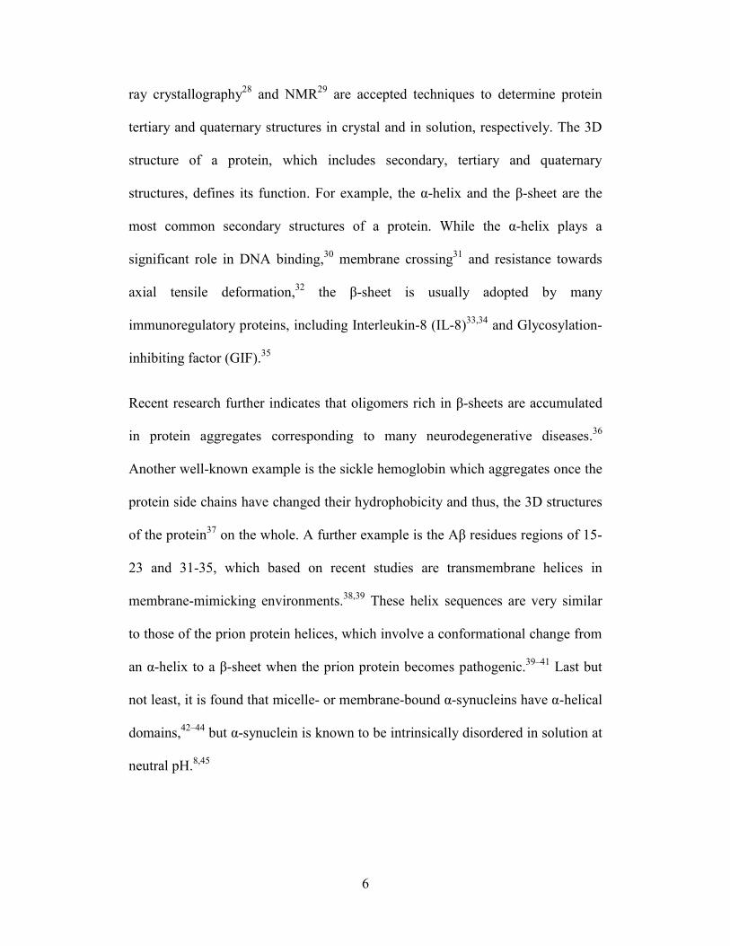
1.2.4 Monitoring protein aggregation in vitro and in vivo
Research monitoring protein aggregation in vitro and in vivo can reveal optimized
environments for protein aggregation/disaggregation and the molecular
mechanisms of protein misfolding and aggregation processes. A variety of
techniques have been utilized in this area: FCS,46
image correlation spectroscopy
(ICS),47
and molecular probes such as thioflavin-T (ThT) and 8-anilino-1-
naphthalene-sulfonate, which can non-specifically bind to fibrillar aggregates.48
For instance, by using ThT assays, scientists reveal that the aggregation of Aβ,
PrPSc and α-synuclein in vitro and in vivo evolve according to the nucleation-
dependent polymerization models,49–51
which indicates that both the initial
monomer concentration and the nucleus size determine the lag time (𝑡𝑑) and half
time ( 𝑡1/2) of the aggregation process.52
Subsequently, FCS experiments
demonstrate that Aβ multimerization is a concentration-dependent53
reaction and
0.2% sodium dodecyl sulfate (SDS) can be used to prevent prion protein from
aggregating.54
In 1998, Pitschke et al. proposed using FCS to detect Aβ
aggregates in the cerebrospinal fluid of Alzheimer’s patients, which became a
pillar for future medical applications.55
Other than the techniques mentioned
above, numerous approaches are also utilized in aggregation-prone protein
studies, such as mass spectrometry (MS), FRET and single-molecule force
spectroscopy (smFS).
8
1.3 α-Synuclein
1.3.1 Research about α-synucleins (1997-2008)
α-Synuclein was first discovered in 1988, quickly followed by the identification
of specific mutations of α-synclein as the chief “culprits” for Parkinson’s diseases
in 1997.56
Thenceforth, our understanding of α-synuclein greatly improved over
the ten years that followed. Most information can be summarized below into four
aspects: (i) the native function of α-synuclein in cells; (ii) the primary structure of
α-synuclein; (iii) the factors that can induce or inhibit α-synuclein aggregation;
and (iv) the identification of the toxic species in the aggregation process.
The native α-synucleins are abundantly found in the terminal of neurons in the
brain and the spinal cord, and their original functions are thought to be one of
support of the plasticity of synaptic membranes,57
to mediate the synaptic function
of neurons, such as vesicular releasing and recycling,58,59
to participate in the
regulation of neuronal apoptosis, including protecting neurons from neuronal
apoptotic stimuli,60
and to act as a molecular chaperone.61
However, the α-
synucleins arising from gene mutation are found to cause neuron death, thus
leading to Parkinson’s disease. For example, scientists have found that 85% of
patients whose neurons expressed α-synuclein A53T mutants (the alanine located
at residue 53 of native α-synuclein are substituted by threonine) gained symptoms
of Parkinson’s disease.62
The other two human α-synuclein gene mutations related
to familial Parkinson’s diseases are A30P and E46K.63
The primary structure of a wild-type α-synuclein is well known; its monomer has
140 residues, which consists of a positive charged N-terminus, a negative charged
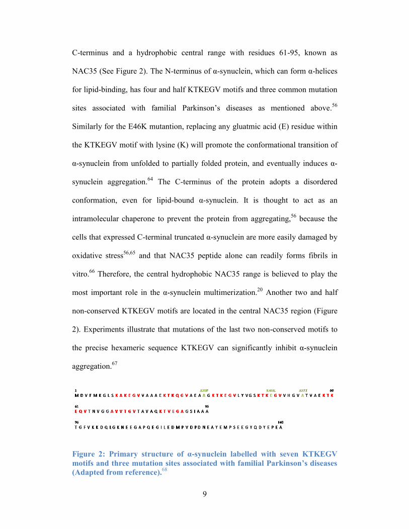
9
C-terminus and a hydrophobic central range with residues 61-95, known as
NAC35 (See Figure 2). The N-terminus of α-synuclein, which can form α-helices
for lipid-binding, has four and half KTKEGV motifs and three common mutation
sites associated with familial Parkinson’s diseases as mentioned above.56
Similarly for the E46K mutantion, replacing any gluatmic acid (E) residue within
the KTKEGV motif with lysine (K) will promote the conformational transition of
α-synuclein from unfolded to partially folded protein, and eventually induces α-
synuclein aggregation.64
The C-terminus of the protein adopts a disordered
conformation, even for lipid-bound α-synuclein. It is thought to act as an
intramolecular chaperone to prevent the protein from aggregating,56
because the
cells that expressed C-terminal truncated α-synuclein are more easily damaged by
oxidative stress56,65
and that NAC35 peptide alone can readily forms fibrils in
vitro.66
Therefore, the central hydrophobic NAC35 range is believed to play the
most important role in the α-synuclein multimerization.20
Another two and half
non-conserved KTKEGV motifs are located in the central NAC35 region (Figure
2). Experiments illustrate that mutations of the last two non-conserved motifs to
the precise hexameric sequence KTKEGV can significantly inhibit α-synuclein
aggregation.67
Figure 2: Primary structure of α-synuclein labelled with seven KTKEGV
motifs and three mutation sites associated with familial Parkinson’s diseases
(Adapted from reference).68
10
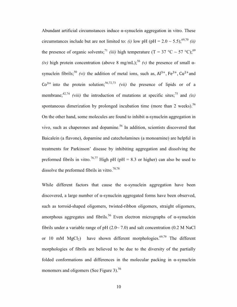
Abundant artificial circumstances induce α-synuclein aggregation in vitro. These
circumstances include but are not limited to: (i) low pH (pH = 2.0 ~ 5.5);69,70
(ii)
the presence of organic solvents;71
(iii) high temperature (T = 37 °C ~ 57 °C);69
(iv) high protein concentration (above 8 mg/mL);56
(v) the presence of small α-
synuclein fibrils;50
(vi) the addition of metal ions, such as, Al3+, Fe3+, Cu2+and
Co3+ into the protein solution;56,72,73
(vii) the presence of lipids or of a
membrane;42,74
(viii) the introduction of mutations at specific sites;75
and (ix)
spontaneous dimerization by prolonged incubation time (more than 2 weeks).56
On the other hand, some molecules are found to inhibit α-synuclein aggregation in
vivo, such as chaperones and dopamine.56
In addition, scientists discovered that
Baicalein (a flavone), dopamine and catecholamines (a monoamine) are helpful in
treatments for Parkinson’ disease by inhibiting aggregation and dissolving the
preformed fibrils in vitro.76,77
High pH (pH = 8.3 or higher) can also be used to
dissolve the preformed fibrils in vitro.70,78
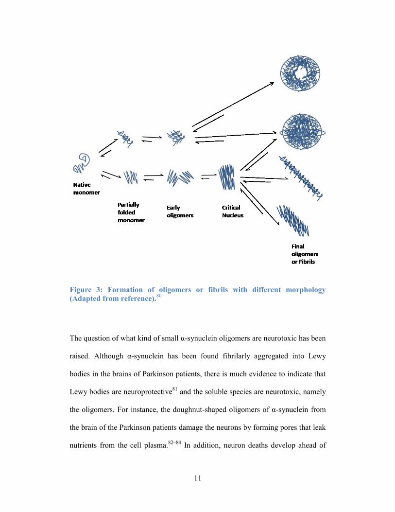
While different factors that cause the α-synuclein aggregation have been
discovered, a large number of α-synuclein aggregated forms have been observed,
such as torroid-shaped oligomers, twisted-ribbon oligomers, straight oligomers,
amorphous aggregates and fibrils.56
Even electron micrographs of α-synuclein
fibrils under a variable range of pH (2.0~ 7.0) and salt concentration (0.2 M NaCl
or 10 mM MgCl2) have shown different morphologies.69,79
The different
morphologies of fibrils are believed to be due to the diversity of the partially
folded conformations and differences in the molecular packing in α-synuclein
monomers and oligomers (See Figure 3).56
11
Figure 3: Formation of oligomers or fibrils with different morphology
(Adapted from reference).80
The question of what kind of small α-synuclein oligomers are neurotoxic has been
raised. Although α-synuclein has been found fibrilarly aggregated into Lewy
bodies in the brains of Parkinson patients, there is much evidence to indicate that
Lewy bodies are neuroprotective81
and the soluble species are neurotoxic, namely
the oligomers. For instance, the doughnut-shaped oligomers of α-synuclein from
the brain of the Parkinson patients damage the neurons by forming pores that leak
nutrients from the cell plasma.82–84
In addition, neuron deaths develop ahead of
12
the formation of detectable fibrils in vitro, which further demonstrate that soluble
media may be more neurotoxic.85
1.3.2 Recent research into α-synuclein (2009-2014)
Based on the above findings, the emphasis of α-synuclein-related research from
2009 to 2014 has shifted to the molecular basis of α-synuclein oligomerzation. To
be more specific, studies on the process of the α-synuclein misfolding and
oligomerization from the molecular perspective can be categorized as the
followings: (i) to identify the important conformational transitions and to
determine the transition rate under “physiological” conditions (10 mM PBS at
neutral pH) and; (ii) to perceive the effects of aggregation-induced factors on the
intermediate molecular structures and the transition rates throughout the
misfolding and oligomerization process; and (iii) to elucidate the misfolding and
oligomerzation pathways at the molecular level. Single-molecule assays including
FCS, ICS, FRET and smFS have become invaluable techniques to study the
aggregation-prone single protein molecules.
Firstly, several α-synuclein conformational transitions, of which the majority
occurred in the N-terminal and NAC35 region, have been seen under
“physiological” conditions. In 2012, Cremades et al. discovered there was a
conformational change between newly formed oligomers and oligomers that were
proteinase-K-resistant under “physiological” conditions by using smFRET, and its
transition rate was ~5 × 10⁻⁶s−1 (5 × 10⁻⁶ moles of oligomers A convert to
oligomers B per second).78
In the same year, Raussens et al. used attenuated total
reflectance – Fourier-transform infrared (ATR – FTIR) spectroscopy to detect the
13
secondary structures in both α-synuclein oligomers and fibrils formed by
spontaneous aggregation over prolonged incubation times. Structures rich in
antiparallel β-sheet were found in the α-synuclein oligomers, while parallel β-
sheets ranging from residues 38-95 were detected in its final fibrilisation.68
In
2014, by using smFS, Neupane et al. discovered ~ 5 metastable transition states
for the α-synuclein monomer, ~ 15 for the dimer and ~20-25 for the tetramer.
Those metastable structures lasted for ~10−1±0.5s before the protein unfolded
again, which further demonstrated that α-synuclein is intrinsically disordered.86
Secondly, numerous experiments have explored the effects of aggregation-
inducing factors on the intermediate molecular structures. For example, two
antiparallel α-helices of α-synuclein can be assembled to “grab” the micelle of a
fatty acid found in neurons of the brain.44,87
In 2010, Trexler et al. discovered that
the α-synuclein monomer was globular, because, while the distances between its
residue 130 and residues 9, 33, 54, 72, 92 were almost the same at the neutral pH,
all the distances were shortened when the pH is lowered to 3.0, with the exception
of the distance between residues 9 and 130. By using smFRET, the C-terminal of
α-synuclein was shown to fold toward its NAC35 region at pH = 3.0. Trexler et al.
explained that low pH greatly changed the charge distributions of the C-terminus
and destroyed its original interactions, which may be helpful to shield the NAC35
region from aggregation. Therefore, the closer proximity of each hydrophobic
NAC35 region driven by C-terminus folding leads to faster α-synuclein
oligomerization at pH = 3.88
Many other researchers agreed with the idea that
aggregation-induced factors can destroy α-synucleins’ original features including
14
long-range interactions, electrostatic interactions, low hydrophobicity and high
net charge, all of which help to shield the protein from aggregation.43,81,89
Uversky
gives a further explanation: the normal α-synuclein is a natively unfolded protein,
so it can possess unstable secondary and tertiary structures as needs dictate for its
dynamic functions. However, the aggregation-inducing factors trap the natively
unfolded α-synuclein into a specific secondary structure, this causes the native
function of unfolded α-synuclein to be lost.56
Furthermore, partially folded α-
synuclein proteins with specific secondary structures have the potential to act as a
tightly packed nucleus that largely reduces the lag time of the aggregation
phenomenon.90
Consistent with this hypothesis, more partially folded α-
synucleins were found to populate under the environments mentioned above
which are able to induce neurotoxic fibrillation, such as low pH69
, high
temperature,69
the presence of metal ions,73
the presence of SDS44
and so forth.
Lastly, nucleation-dependent polymerization is thought to be a good model to
describe α-synuclein misfolding and the oligomerzation process at the molecular
level. The nucleation-polymerization model indicates that the initial step of the α-
synuclein aggregation process, being the addition of monomers, is
thermodynamically unfavourable and the final step of forming fibrils is based on a
critical nucleus which is thermodynamically favourable.91
Therefore, the critical
nucleus is transient but its formation becomes the rate-limiting step of the whole
polymerization process. These critical nuclei are believed to be highly associated
with the cytotoxic oligomers. More and more research has then shifted towards
the study of the structure, cytoxicity of α-synuclein oligomers and their ability to
15
act as a critical nucleus. Recent studies identified several oligomeric structures
and recognized their cellular toxicity. For example, donut-shaped oligomers were
discovered when α-synuclein monomer concentration were above a specific
concentration (8 mg/mL), where they then are potential cytotoxic by
permeabilization of the membrane.92
Annular and spherical oligomers of Ca2+-
binding α-synuclein were discovered to increase the aggregation rate of the
protein.93
Smaller spherical oligomers of Fe3+ -binding α-synuclein in the
presence of ethanol are SDS-resistant but they can form ion-permeable pores in a
lipid bilayer.94
Although the majority of α-synuclein oligomers are cytotoxic and
able to accelerate fibril formation, nontoxic oligomers have also been discovered,
some of which are even able to inhibit fibril formations! For instance, the globular
α-synucleins oligomers stabilized by the flavonoid baicalein are able to greatly
slow down the fibrillation and found to show mild effect on the membrane
surface.90
Moreover, α-synucleins oligomers oxidized by methionine completely
inhibit the fibrillation of non-oxidized α-synuclein at neutral pH.95
1.4 My research objectives
Knowledge of the structure and the cell cytotoxicity of small α-synuclein
oligomers, together with the molecular mechanisms of their formation and the
molecular mechanism of how they shorten the aggregation lag time are still
sparse. As the critical nucleus is transient and difficult to separate from cell in
vitro, an engineered α-synuclein dimer, tetramer and octamer were made in the
lab by tandem linking a repeated monomer with three-amino-acid peptide linker
(GSG).86
To understand whether these engineered α-synuclein oligomers can act
16
as or convert to a critical nucleus in vitro, I aimed to monitor the aggregation
processes of all engineered α-synuclein oligomers constructs in solution. To
achieve this goal, the following research objectives were completed: (i) to
characterize the sizes of α-synuclein monomers and the engineered oligomers by
measuring their hydrodynamic diameters under phosphate-buffered saline (PBS)
at pH = 7.4; (ii) to study the effects of the engineered α-synuclein oligomers on
the monomer fibrillations (acceleration or inhibition); and (iii) to compare and
contrast the kinetics between the self-aggregation (aggregations of the same
construct of α-synuclein) and the cross-aggregation (aggregation of the
monomeric and oligomeric α-synucleins). In general, there are two ways to
experimentally observe proteins aggregation. One is to monitor the increase of the
hydrodynamic sizes of the targeted proteins over time. The other is to detect the
fractions of the proteins that are used to form aggregates as a function of
incubation time. The latter one will be applied in my research.
17
Chapter 2: Methodology and Theory
2.1 Techniques used in protein aggregation studies
The techniques that have been used to monitor protein aggregation in solution
include but are not limited to: (i) SDS-PAGE and Western blot analysis with
chemiluminescence detection; (ii) Size-exclusion chromatography; (iii) Dynamic
light scattering; (iv) ThT assay; (v) In-line Raman spectroscopy; and (vi)
Fluorescence spectroscopy. In this Chapter, the fundamental of some common
techniques will be reviewed, and their pros and cons in protein aggregates studies
will be discussed.
2.1.1 SDS-PAGE
SDS-PAGE refers to sodium dodecyl sulfate-polyacrylamide gel electrophoresis.
SDS is commonly used to denature the 3D structure of a protein so that the
protein becomes one linear amino acid chain with the same negative charges per
unit mass. SDS-PAGE is a technique that is widely used to separate proteins
based on differences in molecular mass. An electric field is used in SDS-PAGE to
pull the charged amino acid chains through the gel and the protein with larger
molecular mass moves slower. Once the diverse proteins are separated from each
other, all protein bands are transferred from the gel to a nitrocellulose membrane
and a specific dye is used to stain the band of interest in the membrane. This
method enables us to quickly distinguish the α-synuclein monomer and oligomers
in a small amount of clinical sample. For example, Baba et al. utilized this method
18
to prove the existence of full-length α-synuclein, truncated α-synuclein and
insoluble aggregates in the Lewy bodies purified from the brain of patients with
Parkinson’s disease. The anti-synuclein antibodies MAb, LB509 and antiserum
259 were used to specifically bind to the purified human α-synuclein.96
There are
several disadvantages of this method. First of all, the results are non-quantified
and have limited reproducibility. Second, the dynamic process of α-synuclein
aggregation cannot be captured early using this method.
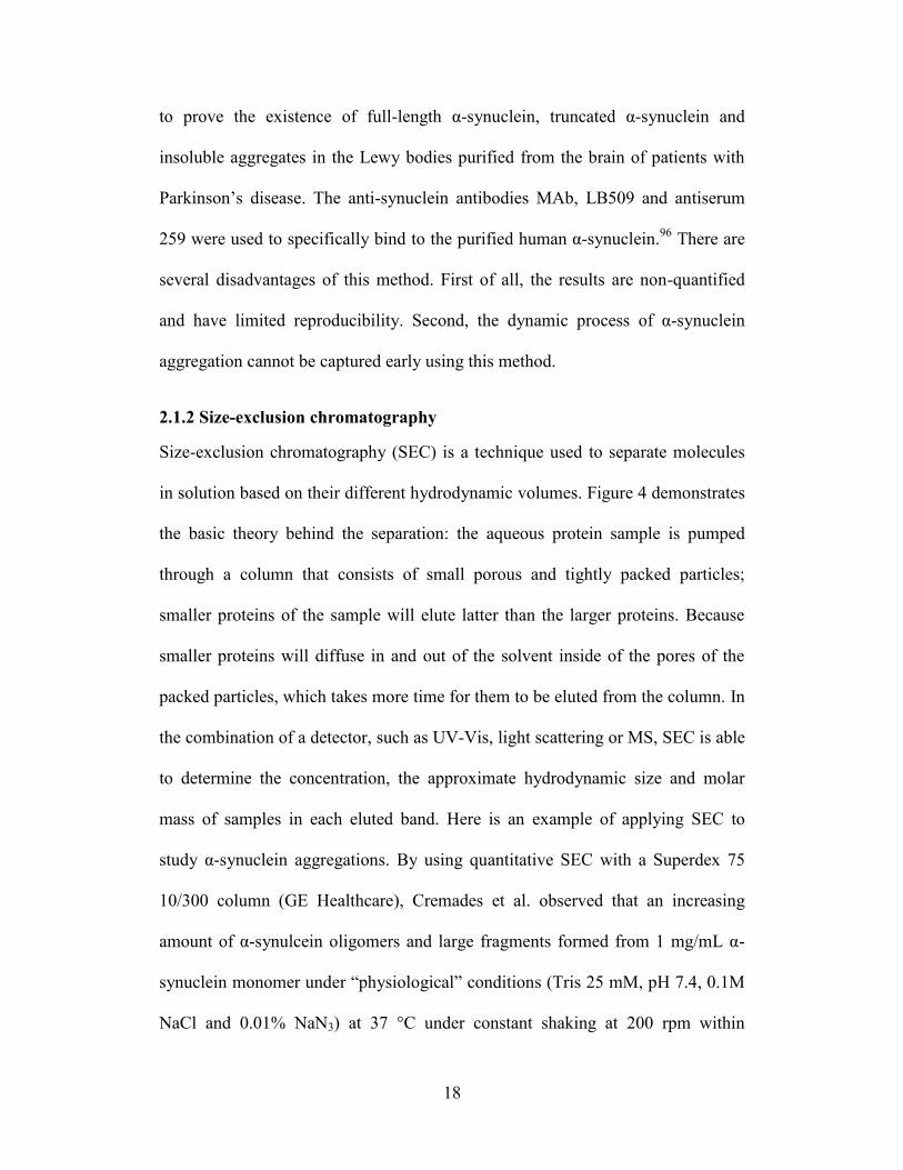
2.1.2 Size-exclusion chromatography
Size-exclusion chromatography (SEC) is a technique used to separate molecules
in solution based on their different hydrodynamic volumes. Figure 4 demonstrates
the basic theory behind the separation: the aqueous protein sample is pumped
through a column that consists of small porous and tightly packed particles;
smaller proteins of the sample will elute latter than the larger proteins. Because
smaller proteins will diffuse in and out of the solvent inside of the pores of the
packed particles, which takes more time for them to be eluted from the column. In
the combination of a detector, such as UV-Vis, light scattering or MS, SEC is able
to determine the concentration, the approximate hydrodynamic size and molar
mass of samples in each eluted band. Here is an example of applying SEC to
study α-synuclein aggregations. By using quantitative SEC with a Superdex 75
10/300 column (GE Healthcare), Cremades et al. observed that an increasing
amount of α-synulcein oligomers and large fragments formed from 1 mg/mL α-
synuclein monomer under “physiological” conditions (Tris 25 mM, pH 7.4, 0.1M
NaCl and 0.01% NaN3) at 37 °C under constant shaking at 200 rpm within
19
15~150 hours.78
However, one major drawback of SEC prevents us from studying
α-synuclein aggregation: the size exclusion column has a comparatively narrow
working range and all α-synuclein oligomers elute as one band. Therefore, it is
impossible to figure out if different kinds of α-synuclein oligomers are formed
during the incubation. Moreover, dramatic protein loss is observed during each
experiment. In my research work, size-exclusion chromatography is only used to
remove excess free dye from the labelled α-synuclein by using Sephadex G-25
desalting column.
Figure 4: Principle of SEC (Adapted from reference).97
20
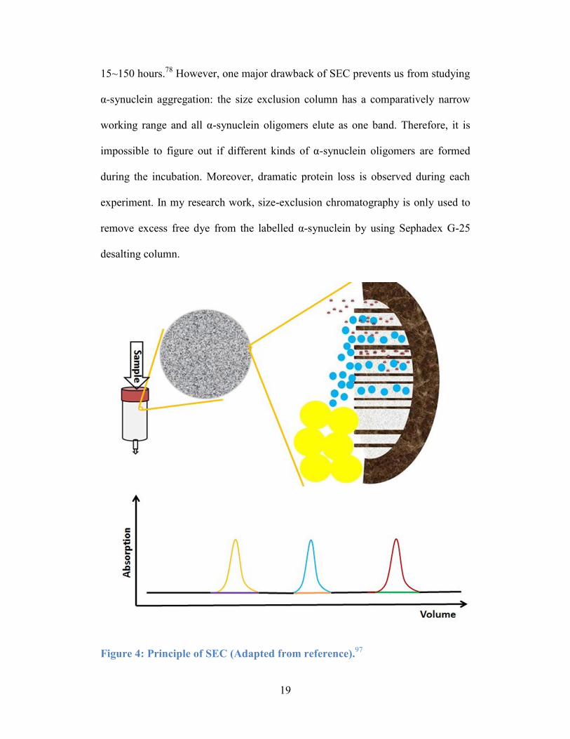
2.1.3 Dynamic light scattering (DLS)
DLS is widely used to determine the hydrodynamic radius of a particle ranging
from 0.3 nm to 10.0 μm in a monodisperse solution. As shown in Figure 5,
monochromatic and coherent light hits the moving particles with the same size
and the scattered lights at certain angle are detected to generate a spectrum of the
fluctuations of scattering light intensity over time.
Figure 5: Principle of DLS.
With the assumption that all particles in a sample move by Brownian motion, the
smaller particles move faster and thus their scattering light fluctuate faster
compared with those of larger particles. The correlation function of DLS can be
defined as98
𝐆(𝛕) = ∫ 𝑰(𝒕)𝑰(𝒕 + 𝝉)𝒅𝒕∞
𝟎 (1)
21
where 𝐼(𝑡) is the scattered light intensity, and a plot of 𝐺(𝑡) as a function of time
can be drawn. This plot is also called a correlogram. Equation (2) demonstrates
that the decay rate of the correlogram is related to the diffusion coefficient (𝐷) of
the measured particle.
∫ 𝑰(𝒕)𝑰(𝒕 + 𝝉)𝒅𝒕 = 𝑩 + 𝑨𝒆−𝟐𝒒𝟐𝑫𝝉∞
𝟎 (2)
In Equation (2), 𝐵 and 𝐴 are the baseline and the amplitude of the correlogram,
respectively. The parameter, 𝑞, is the scattering vector which is affected by the
solvent refractive index, laser wavelength and the scattering angle, and 𝐷 is the
diffusion coefficient of the particle of interest. Once 𝐷 is known, the
hydrodynamic radius of the particle can be calculated based on the Stokes-
Einstein equation (More details in Section 2.2.3).22
Previous research has used
DLS to monitor the formation of α-synuclein oligomers. For instance, Fink et al.
obtained the hydrodynamic radius of the mutated α-synuclein monomer Y39W
(3.1 ± 0.2 nm) by DLS and observed the formation of its oligomeric species with
the hydrodynamic radius equal to 22 ± 2 nm after 3 hours of incubation (20 mM
phosphate buffer containing 150 mM NaCl at 37 °C and pH 7.4)99
. They also
showed that the concentration of the oligomeric species increased to 15% of the
total protein concentration after 18 hours of incubation and then decreased.99
Compared with the techniques mentioned above, DLS is easy to use and its results
are highly reproducible. However, the drawback of using DLS in protein
aggregation study is that the heavily aggregated protein solution being incubated
for a very long time becomes too polydisperse to be accurately interpreted. In my
22
research work, DLS is used to measure the hydrodynamic diameters of the native
α-synuclein monomer, as well as the engineered α-synuclein dimer, tetramer and
octamer. Then, the DLS data are used to validate those obtained from FCS.
2.2 Fluorescence Spectroscopy
Fluorescence Spectroscopy is a technique which has noticeable advantages in the
protein aggregation studies compared with the other techniques summarized
above. First of all, it allows us to monitor the protein misfolding and aggregation
process both in vitro and vivo at very low sample concentration (~ nM) with small
volume (~ several 100 µL). Second, a variety of information including the
concentration of a fluorescent sample, the averaged hydrodynamic radius of the
fluorescent particles in the sample and even the averaged molar fraction of a
specific component in the fluorescent particles can be obtained. Because of its
high sensitivity, high precision and multifunction, fluorescence spectroscopy can
not only be used to detect the changes of the hydrodynamic sizes of α-synuclein
within a long incubation time, it can also be used to monitor the dynamic changes
in the fractions of α-synuclein monomers contributed in the aggregation over long
incubation time. Therefore, fluorescence spectroscopy is the main technique used
to study the self-aggregation and cross-aggregation between α-synuclein
monomer and the engineered oligomers in solution in our work.
2.2.1 Structure of a fluorescence microscope
A fluorescence microscope can “see” fluorescent molecules in solution.
Experiments can be performed with one excitation only or with both excitations
simultaneously. A simplified fluorescence microscope with specific excitation
23
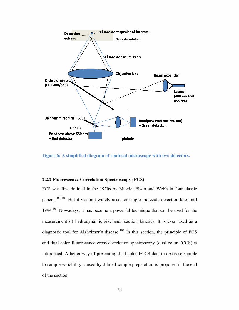
wavelengths and dichroic mirrors used in my research is shown in Figure 6. The
filtered excitation light of 488 nm and 633 nm is first expanded by a beam
expander, and then is reflected along the optical axis to the edges of the objective
lens by hitting a dichroic mirror (HFT 488/633) at 45 degrees. Next, the objective
lens focuses the excitation light onto a sample solution to form a specific
detection volume. The fluorescent species of interest diffuse in the detection
volume are excited and emit the fluorescence light as well as the scattered and
reflected light along the optical axis to hit back onto the dichroic mirror (HFT
488/633). However, only the emitted fluorescence light can pass through the
dichroic mirror and the scattered and reflected light from the sample will be
reflected by 90°. Then another dichroic mirror (NFT 635) allows wavelengths
above 635 nm to pass through and the rest of wavelengths are reflected 90
degrees. The pass-through light passes through a high pass filter (LP 650 nm) and
hits a detector, which is the “red detector”. Another band pass filter (BP 505 nm ~
550 nm) is also set before the other detector, which refers to the “green detector”,
so that only wavelength at 505 nm ~ 550 nm hits the detector.
24
Figure 6: A simplified diagram of confocal microscope with two detectors.
2.2.2 Fluorescence Correlation Spectroscopy (FCS)
FCS was first defined in the 1970s by Magde, Elson and Webb in four classic
papers.100–103
But it was not widely used for single molecule detection late until
1994.104
Nowadays, it has become a powerful technique that can be used for the
measurement of hydrodynamic size and reaction kinetics. It is even used as a
diagnostic tool for Alzheimer’s disease.105
In this section, the principle of FCS
and dual-color fluorescence cross-correlation spectroscopy (dual-color FCCS) is
introduced. A better way of presenting dual-color FCCS data to decrease sample
to sample variability caused by diluted sample preparation is proposed in the end
of the section.
25
The principle of FCS
Fluorescence autocorrelation spectroscopy is a correlation analysis method for the
study of fluorescence intensity fluctuation within a detection volume (similar in
principle to DLS). The best sample for fluorescence autocorrelation spectroscopy
contains only one fluorescent species or two independent fluorescent species with
at least 10 fold differences in their molecular weights. This method can be
ultimately used to determine the concentration of the fluorescent sample, as well
as the hydrodynamic radius of a fluorescent particle in the sample.
The theory of FCS is based on two assumptions.106
First, the fluorescent
molecules of the FCS sample are in Brownian motion and can freely diffuse
through the detection volume. Second, quantities of fluorescent molecules that
diffuse through the detection volume follow a Poisson distribution,
𝑷(𝒌; 𝝁) = 𝝁𝒌×𝒆−𝝁
𝒌! (3)
where 𝑃(𝑘; 𝜇) refers to the probability of the cases for exactly k fluorescent
molecules occurring in the detection volume, when 𝜇 of fluorescent molecules
detected in average in the same region. The most important characteristic of a
Poisson experiment is that the variance of the successes (𝜎2) is equal to its mean:
𝝈𝟐 = 𝝁 (4)
26
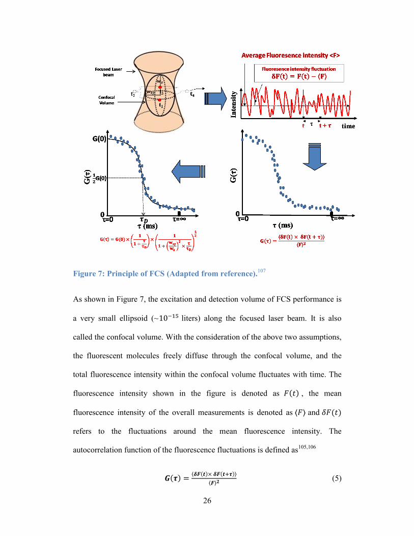
Figure 7: Principle of FCS (Adapted from reference).107
As shown in Figure 7, the excitation and detection volume of FCS performance is
a very small ellipsoid (~10−15 liters) along the focused laser beam. It is also
called the confocal volume. With the consideration of the above two assumptions,
the fluorescent molecules freely diffuse through the confocal volume, and the
total fluorescence intensity within the confocal volume fluctuates with time. The
fluorescence intensity shown in the figure is denoted as 𝐹(𝑡) , the mean
fluorescence intensity of the overall measurements is denoted as ⟨𝐹⟩ and 𝛿𝐹(𝑡)
refers to the fluctuations around the mean fluorescence intensity. The
autocorrelation function of the fluorescence fluctuations is defined as105,106
𝑮(𝝉) =⟨𝜹𝑭(𝒕)× 𝜹𝑭(𝒕+𝝉)⟩
⟨𝑭⟩𝟐 (5)
27
where 𝑡 is the actual measured time when 𝛿𝐹(𝑡) is obtained, and 𝜏 is the time
difference between one measurement and the other measurement, usually range
from 0.01 ms to 0.1 s. ⟨𝛿 𝐹(𝑡) × 𝛿𝐹(𝑡 + 𝜏)⟩ refer to the average value of the
𝛿 𝐹(𝑡) × 𝛿𝐹(𝑡 + 𝜏) throughout the overall data accumulation time.
Once the autocorrelation function of the fluorescence fluctuation is obtained, a
specific equation is used to fit the autocorrelation function as shown in the last
plot of Figure 7. For the case that only one fluorescent species translationally
diffuses in a 3D detection volume, the following fitting equation is used105,106
𝑮(𝝉) = 𝑮(𝟎) × (𝟏
𝟏+𝝉
𝝉𝑫
) × (𝟏
𝟏+(𝒘𝒙𝒚
𝒘𝒛)
𝟐×
𝝉
𝝉𝑫
)
𝟏
𝟐
(6)
where 𝜏 and 𝐺(𝜏) are variables obtained from the experiments, 𝐺(0) and 𝜏𝐷 are
the important parameters generated by fitting, their physical meanings are
described below in detail. The parameter, 𝑤𝑥𝑦 , can also be found in Figure 7;
it refers to the equatorial radius of the confocal volume. The parameter, 𝑤𝑧, is the
polar radius of the confocal volume which is along the direction of propagation of
the focused laser beam. Both 𝑤𝑥𝑦 and 𝑤𝑧 are independent of the sample, and they
only change when different excitation wavelengths are used. Therefore, the ratio
of 𝑤𝑥𝑦 and 𝑤𝑧 is a constant during the measurements.
Physical meaning of the important parameters in FCS
Two important parameters can be generated from the fitting of the autocorrelation
function: 𝐺(0) and 𝜏𝐷. 𝐺(0) can be used to deduce the actual concentration of a
28
fluorescent species in the sample and 𝜏𝐷 can be used to calculate the
hydrodynamic radius of the species.
𝐺(0) is the amplitude of a correlation function when τ is equal to zero. In
practice, 𝐺(0) is equal to the reciprocal of average observed number of
fluorophores within a confocal volume as shown in Equation (7)106
𝑮(𝟎) =𝟏
⟨𝑵⟩ (7)
Once ⟨𝑁⟩ is known, the mean concentration of a FCS sample can be calculated by
⟨𝒄⟩ = ⟨𝑵⟩
𝑽𝒆𝒇𝒇∙𝑵𝑨 (8)
where 𝑁𝐴 is the Avogadro constant. 𝑉𝑒𝑓𝑓 is the effective confocal volume which
is calculated based on the the equatorial radius (𝑤𝑥𝑦) and the polar radius (𝑤𝑧) of
the confocal volume by106
𝑽𝒆𝒇𝒇 = 𝝅𝟑
𝟐𝒘𝒙𝒚𝟐 𝒘𝒛 (9)
There are two important requirements for a reliable FCS measurement. First, a
FCS sample has to be measured at the nanomolar scale to ensure only a few of
fluorophores are detected in the confocal volume throughout the overall data
accumulation time. Second, the effective confocal volume has to be minimized to
the femtoliter range (~ 1 𝑓𝐿 ). Only by following these requirements, the
fluorescence fluctuation caused by a single fluorophore translationally diffusing
in/out of the confocal volume is significant relative to the noise.
29
Another important fitting parameter is the diffusion time (𝜏𝐷), which is equal to
the time needed when 𝐺(𝜏) = 1
2𝐺(0), as shown in Figure 7. The translational
diffusion coefficient (𝐷) of a fluorescent molecule can be calculated based on its
measured diffusion time as below
𝑫 =𝒘𝒙𝒚
𝟐
𝟒×𝝉𝑫 (10)
Moreover, the relationship between the hydrodynamic radius (𝑅) of a fluorescent
molecule and its translational diffusion coefficient ( 𝐷 ) is known as Stokes-
Einstein equation, Equation (11)
𝑹 =𝒌𝑻
𝟔𝝅𝜼𝑫 (11)
where 𝑘 = 1.38 × 10⁻²³ m2kg
s2K is the Boltzmann constant. T is the temperature
during a FCS measurement, and 𝜂 is the viscosity of the buffer used in the
meansurement. To sum up, FCS is a technique to obtain the concentration of one
kind of fluorescent species as well as its average hydrodynamic diameter in a
sample solution.
Two-component FCS fitting equation
For the case that two independent fluorescent species laterally diffusing in the
sample, the equation described autocorrelation function of total fluorescence
fluctuations is the same, but a new fitting equation is used.106
The mathematic
equation is shown in Equation (12)
30
𝑮(𝝉)
𝑮(𝟎) =
𝑵𝟏
𝑵𝑫𝟏(𝝉) +
𝑵𝟐
𝑵𝑫𝟐(𝝉) (12)
𝑫𝒊(𝝉) = (𝟏
𝟏+𝝉
𝝉𝑫𝒊
) × (𝟏
𝟏+(𝒘𝒙𝒚
𝒘𝒛)
𝟐×
𝝉
𝝉𝑫𝒊
)
𝟏
𝟐
(13)
where 𝐷1(𝜏) and 𝐷2(𝜏) as defined in Equation (13), are a part of the correlation
function that contains information about the diffusion time of the two fluorescent
species. The parameters, 𝑁1 and 𝑁2 correspond to the number of the fluorescent
species 1 and 2 observed in the confocal volume. 𝑁 is the sum of 𝑁1 and 𝑁2 .
Consequently, 𝑁1
𝑁 refers to the mole fraction of species 1. In my research, two-
component correlation fitting equation is often used, because the free dye (the dye
without binding to any protein) cannot be completely removed from the labelled
protein solution. Therefore, the fluorescent species 1 refers to the free dye and the
fluorescent species 2 refers to the labelled protein. Combined with Equations (8),
(9), (10) and (11), the concentration and the hydrodynamic radius of a labelled
protein are still able to be obtained by a FCS experiment.
Other fitting factors needed to be considered
In a real FCS experiment, many other factors are taken into consideration to
properly fit a FCS curve. These include the rotational diffusion of a fluorophore
and its dynamic fluorescence property. Their influences on the correlation
function of the fluorescence fluctuations are discussed here and are shown in
Figure 8 (b).
31
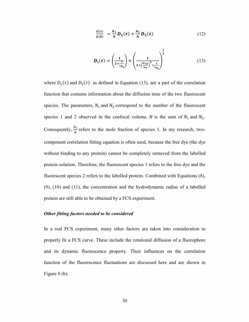
Figure 8: (a) Autocorrelation function of two component translational
fluctuations; (b) Autocorrelation function for one component translational
fluctuation with triplet and rotational diffusion.
First, an unobvious decay is usually found in an autocorrelation function around
𝜏 = 10−8~10−7s. This decay is formed when the measured fluorophores rotate
while they cross the confocal volume. This is because laser is polarized and it is
only be detected if detector is polarized. Therefore, the rotation of fluorophores
can usually be neglected. Moreover, the rotational correlation time is much
shorter than the diffusional correlation time. Second, a triplet shoulder is
commonly observed in an autocorrelation function around 𝜏 = 10−7~10−6s. This
phenomenon is caused by the forbidden transition of the fluorophores to the triplet
state. In other words, a few of fluorophores, which are excited to the triplet state,
are dark while they laterally pass through the confocal volume.108
In order to
avoid these problems which may cause an improper fitting, FCS curves in my
research are usually fitted starting at 𝜏 = 10−6 s.
32
2.2.3 Dual-color FCCS
Dual-color fluorescence cross-correlation spectroscopy (Dual-color FCCS) is an
advanced correlation analysis method for the translational diffusions of multiple
components in a system. The main advantage of dual-color FCCS is that it allows
us to distinguish any of two species even if there is only a small molecular weight
difference between the two species.109
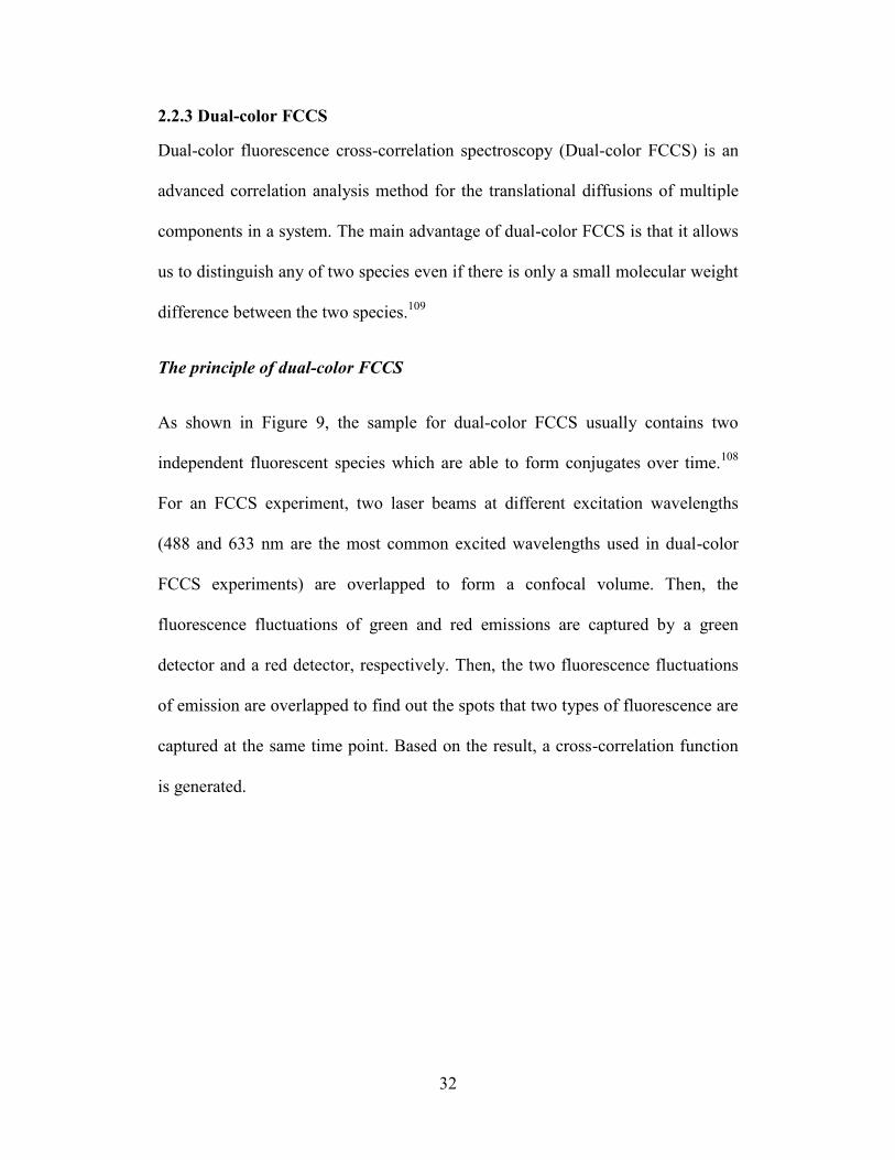
The principle of dual-color FCCS
As shown in Figure 9, the sample for dual-color FCCS usually contains two
independent fluorescent species which are able to form conjugates over time.108
For an FCCS experiment, two laser beams at different excitation wavelengths
(488 and 633 nm are the most common excited wavelengths used in dual-color
FCCS experiments) are overlapped to form a confocal volume. Then, the
fluorescence fluctuations of green and red emissions are captured by a green
detector and a red detector, respectively. Then, the two fluorescence fluctuations
of emission are overlapped to find out the spots that two types of fluorescence are
captured at the same time point. Based on the result, a cross-correlation function
is generated.
33
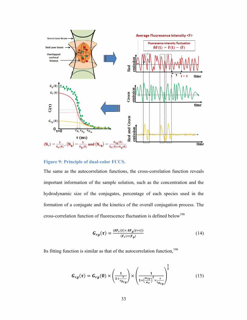
Figure 9: Principle of dual-color FCCS.
The same as the autocorrelation functions, the cross-correlation function reveals
important information of the sample solution, such as the concentration and the
hydrodynamic size of the conjugates, percentage of each species used in the
formation of a conjugate and the kinetics of the overall conjugation process. The
cross-correlation function of fluorescence fluctuation is defined below106
𝑮𝒓𝒈(𝝉) =⟨𝜹𝑭𝒓(𝒕)× 𝜹𝑭𝒈(𝒕+𝝉)⟩
⟨𝑭𝒓⟩×⟨𝑭𝒈⟩ (14)
Its fitting function is similar as that of the autocorrelation function,106
𝑮𝒓𝒈(𝝉) = 𝑮𝒓𝒈(𝟎) × (𝟏
𝟏+𝝉
𝝉𝑫𝒓𝒈
) × (𝟏
𝟏+(𝒘𝒙𝒚
𝒘𝒛)
𝟐×
𝝉
𝝉𝑫𝒓𝒈
)
𝟏
𝟐
(15)
34
The amplitude of the cross-correlation function equals:
𝑮𝒓𝒈(𝟎) =⟨𝜹𝑭𝒓(𝒕)× 𝜹𝑭𝒈(𝒕)⟩
⟨𝑭𝒓⟩×⟨𝑭𝒈⟩=
⟨𝑵𝒓𝒈⟩
⟨𝑵𝒓⟩×⟨𝑵𝒈⟩ (16)
To rearrange Equation (16):
𝑵𝒓𝒈 =𝑮𝒓𝒈(𝟎)
𝑮𝒓(𝟎)×𝑮𝒈(𝟎) (17)
where ⟨𝑁𝑟𝑔⟩ is the average number of conjugates that can emit both red and green
fluorescence within the overlapped confocal volume, and ⟨𝑁𝑟⟩ is the average
number of species that emit red fluorescence, which includes the red fluorescent
species and all conjugates. Similarly, ⟨𝑁𝑔⟩ includes the green fluorescent species
and all conjugates. Once ⟨𝑁𝑟𝑔⟩ is known, the mean concentration of the
conjugates can be calculated based on Equation (8). One difference is that the
𝑉𝑒𝑓𝑓_𝐶𝑟𝑜𝑠𝑠 now refers to the overlapped effective confocal volume of two laser
beams, which is defined as106
𝑽𝒆𝒇𝒇_𝑪𝒓𝒐𝒔𝒔 = (𝝅
𝟐)
𝟑
𝟐(𝒘𝒙𝒚_𝒓𝒆𝒅
𝟐 + 𝒘𝒙𝒚_𝒈𝒓𝒆𝒆𝒏𝟐 )(𝒘𝒛_𝒓𝒆𝒅
𝟐 + 𝒘𝒛_𝒈𝒓𝒆𝒆𝒏𝟐 )
𝟏
𝟐 (18)
where 𝑤𝑥𝑦_𝑟𝑒𝑑, as shown in Figure 9, is the equatorial radius and 𝑤𝑧_𝑟𝑒𝑑, is the
polar radius of the confocal volume which along the focused red laser beam.
𝑤𝑥𝑦_𝑔𝑟𝑒𝑒𝑛 and 𝑤𝑧_𝑔𝑟𝑒𝑒𝑛 refer to the corresponding radius of the focused green
laser beam. Another difference is that the translational diffusion coefficient of the
combined species (𝐷𝑟𝑔) is calculated as106
𝑫𝒓𝒈 =𝒘𝒙𝒚_𝒓𝒆𝒅
𝟐 +𝒘𝒙𝒚_𝒈𝒓𝒆𝒆𝒏𝟐
𝟖×𝝉𝑫_𝒓𝒈 (19)
35
where 𝝉𝑫_𝒓𝒈refers to the translational diffusion time of the aggregate. The stokes-
Einstein equation, the Equation (11), can also be used here to calculate the
hydrodynamic radius ( 𝑅𝑟𝑔) of the aggregate from its translational diffusion
coefficient (𝐷𝑟𝑔).
Other general factors that need to be considered
In theory, three correlation functions, the last diagram in Figure 9, are exactly the
same if there are only red-green aggregates presenting in the sample. However,
even then, the three correlation functions are rarely the same in reality. There are
two reasons. First, the two lasers beams or their detection volumes do not exactly
overlapped. Second, the effect of green dye to red channel is not negligible.
To solve the former issue, a calibration for FCCS experiments is required.109
To
ensure the overlap of detection volumes, a FCCS test can be done by exciting
Rhodamine 6G with a 488 nm laser beam and receiving its emission by both
Green and Red detection. By comparing the two amplitudes of the autocorrelation
functions with the amplitude of the cross correlation function, it is known whether
the two detections “see” the same spot. To ensure the overlap of lasers, a FCCS
test can be done by exciting a red dye with a 633 nm laser beam and then exciting
the same dye with a 488 nm laser beam. If the two autocorrelation functions have
the same amplitude and diffusion time, it means that two lasers overlap.109
Usually, the width of a laser beam is proportional to its wavelength,110
which will
eventually cause a larger red laser beam and detection volume. In this case,
instead of using ⟨𝑁𝑟⟩, ⟨𝑁𝑔⟩ and ⟨𝑁𝑟𝑔⟩ for the further calculation of the aggregation
36
process, ⟨𝑛𝑟 ⟩, ⟨𝑛𝑔⟩ and ⟨𝑛𝑟𝑔⟩ will be applied. ⟨𝑛𝑟𝑔⟩ is the concentration of the
conjugated fluorescent species observed in the effective cross detection volume,
which is defined as
⟨𝒏𝒓𝒈⟩ =⟨𝑵𝒓𝒈⟩
𝑽𝒆𝒇𝒇𝒓𝒈
=⟨𝑵𝒓𝒈⟩
(𝝅
𝟐)
𝟑𝟐(𝒘𝒙𝒚_𝒓𝒆𝒅
𝟐 +𝒘𝒙𝒚_𝒈𝒓𝒆𝒆𝒏𝟐 )(𝒘𝒛_𝒓𝒆𝒅
𝟐 +𝒘𝒛_𝒈𝒓𝒆𝒆𝒏𝟐 )
𝟏𝟐
(20)
The same for ⟨𝑛𝑟⟩ and ⟨𝑛𝑔⟩,
⟨𝒏𝒓⟩ =⟨𝑵𝒓⟩
𝑽𝒆𝒇𝒇𝒓
=⟨𝑵𝒓⟩
(𝝅
𝟐)
𝟑𝟐∙𝒘𝒙𝒚_𝒓𝒆𝒅
𝟐 ∙𝒘𝒛_𝒓𝒆𝒅
(21)
⟨𝒏𝒈⟩ =⟨𝑵𝒈⟩
𝑽𝒆𝒇𝒇𝒈
=⟨𝑵𝒈⟩
(𝝅
𝟐)
𝟑𝟐∙𝒘𝒙𝒚_𝒈𝒓𝒆𝒆𝒏
𝟐 ∙𝒘𝒛_𝒈𝒓𝒆𝒆𝒏
(22)
The issue that the cross talk of green dye to red channel may not be negligible is
solved when a proper dye system is chosen. the cross talk of green dye to red
channel is negligible when the following condition is fulfilled109
𝑬𝑮𝑮𝑮
𝑬𝑹𝑹𝑹≈ 𝟏 (23)
𝑬𝑮𝑮𝑮
𝑬𝑹𝑮𝑮≈ 𝟐𝟎 (24)
𝑬𝑹𝑹𝑹
𝑬𝑹𝑹𝑮≈ 𝟖 (25)
𝑬𝑹𝑮𝑮+𝑬𝑹𝑹𝑮+𝑬𝑹𝑹𝑹
𝑬𝑹𝑮𝑮≈ 𝟐𝟎 (26)
where 𝐸𝐺𝐺𝐺 refers to the green emission of green dye excited by green laser, 𝐸𝑅𝑅𝑅
refers to the red emission of red dye excited by red laser, ERGG refers to the red

37
emission of green dye excited by green laser and 𝐸𝑅𝑅𝐺 refers to the red emission
of red dye excited by green laser.
38
Chapter 3: Materials and Methods
3.1 Labelling
α-Synuclein preparation. During the experiments, the engineered α-synuclein
dimer, tetramer and octamer are made by tandem linking repeated monomer with
three-amino-acid peptide linker (GSG). In order to specifically label each α-
synuclein with a fluoresence dye, one cysteine was inserted to the C terminal of
each construct. Overall, the α-synuclein monomer and these engineered dimer,
tetramer and octamer with one C-terminal cysteine are my study objects. My
coworker, Meijing Wang, synthesized them by the following procedures. First,
the native monomeric, dimeric tetrameric and octameric α-synuclein expression
constructs were obtained from B-Bridge International. Second, the Site-Directed
Mutagenesis Kit from Agilent Technologies was used to add one cysteine on the
C-terminal of each α-synuclein construct. Once the DNA sequence and the amino
acid sequence of the mutated α-synulcein were confirmed, the plasmid containing
the α-synuclein of interest were inserted into the RosettaTM
2 (DE3) Competent
Cells from EMD Millipore for over expression. Then, osmotic shock was used to
break the cell and release all proteins from the cell. Finally, Ion exchange
chromatography with Q Sepharose medium was used to purify the α-synuclein of
interest from all other proteins and 90% ammonia sulfate were used to precipitate
the purified α-synuclein for labelling or storage at -80 °C. In the following
research, the α-synuclein monomer and its engineered dimer, tetramer and
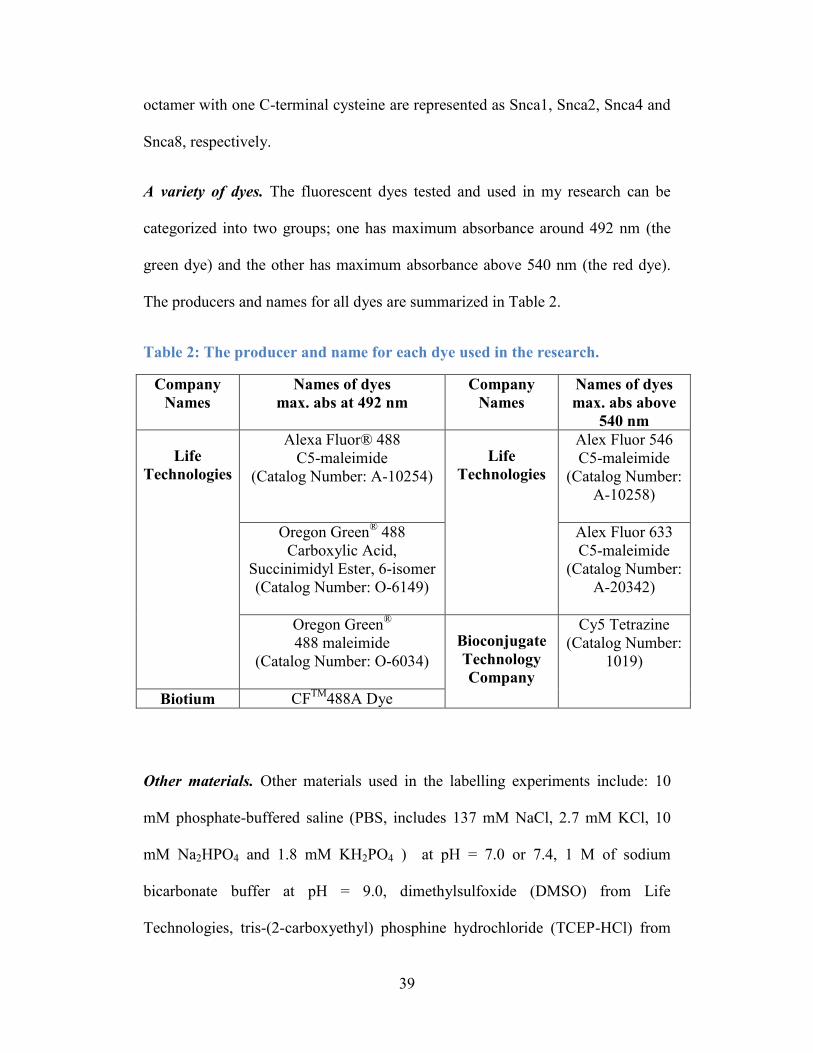
39
octamer with one C-terminal cysteine are represented as Snca1, Snca2, Snca4 and
Snca8, respectively.
A variety of dyes. The fluorescent dyes tested and used in my research can be
categorized into two groups; one has maximum absorbance around 492 nm (the
green dye) and the other has maximum absorbance above 540 nm (the red dye).
The producers and names for all dyes are summarized in Table 2.
Table 2: The producer and name for each dye used in the research.
Company
Names
Names of dyes
max. abs at 492 nm
Company
Names
Names of dyes
max. abs above
540 nm
Life
Technologies
Alexa Fluor® 488
C5-maleimide
(Catalog Number: A-10254)
Life
Technologies
Alex Fluor 546
C5-maleimide
(Catalog Number:
A-10258)
Oregon Green® 488
Carboxylic Acid,
Succinimidyl Ester, 6-isomer
(Catalog Number: O-6149)
Alex Fluor 633
C5-maleimide
(Catalog Number:
A-20342)
Oregon Green®
488 maleimide
(Catalog Number: O-6034)
Bioconjugate
Technology
Company
Cy5 Tetrazine
(Catalog Number:
1019)
Biotium CFTM
488A Dye
Other materials. Other materials used in the labelling experiments include: 10
mM phosphate-buffered saline (PBS, includes 137 mM NaCl, 2.7 mM KCl, 10
mM Na2HPO4 and 1.8 mM KH2PO4 ) at pH = 7.0 or 7.4, 1 M of sodium
bicarbonate buffer at pH = 9.0, dimethylsulfoxide (DMSO) from Life
Technologies, tris-(2-carboxyethyl) phosphine hydrochloride (TCEP-HCl) from
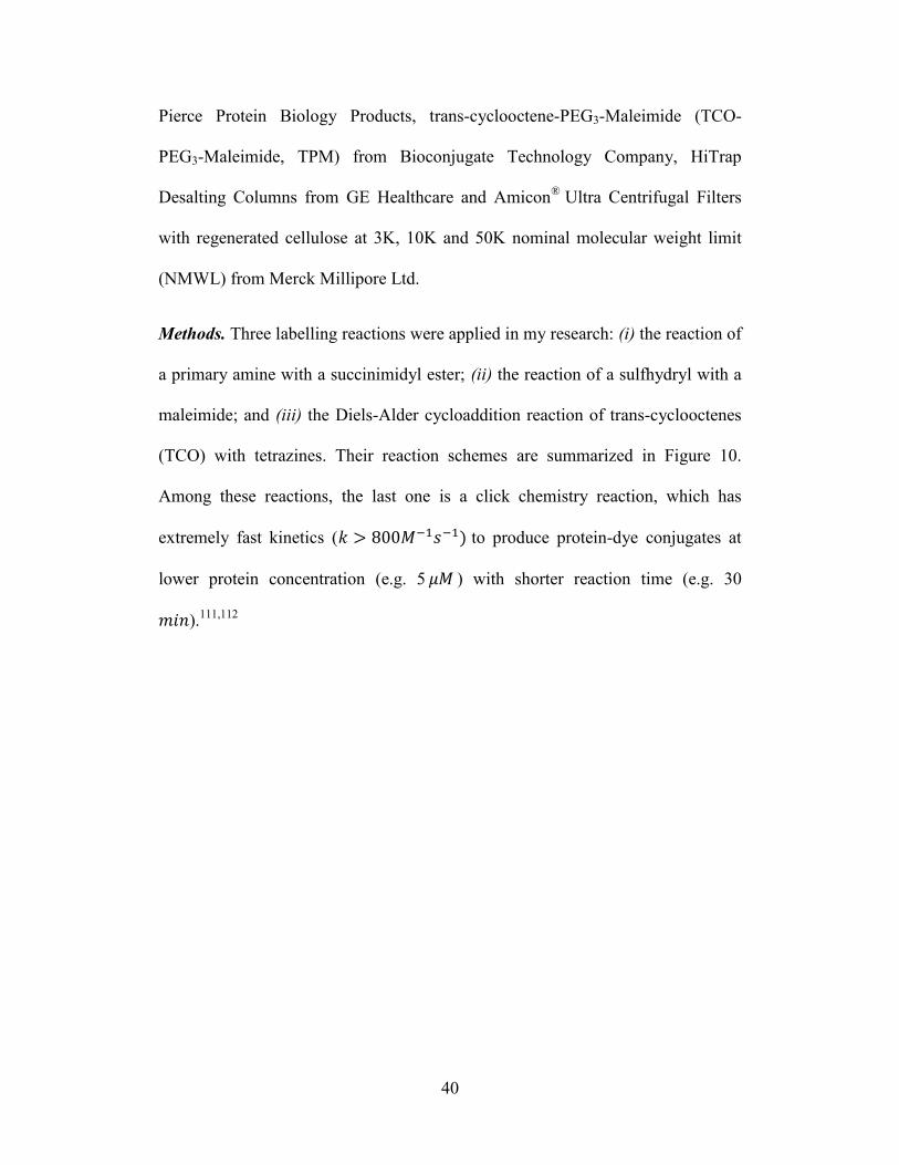
40
Pierce Protein Biology Products, trans-cyclooctene-PEG3-Maleimide (TCO-
PEG3-Maleimide, TPM) from Bioconjugate Technology Company, HiTrap
Desalting Columns from GE Healthcare and Amicon®
Ultra Centrifugal Filters
with regenerated cellulose at 3K, 10K and 50K nominal molecular weight limit
(NMWL) from Merck Millipore Ltd.
Methods. Three labelling reactions were applied in my research: (i) the reaction of
a primary amine with a succinimidyl ester; (ii) the reaction of a sulfhydryl with a
maleimide; and (iii) the Diels-Alder cycloaddition reaction of trans-cyclooctenes
(TCO) with tetrazines. Their reaction schemes are summarized in Figure 10.
Among these reactions, the last one is a click chemistry reaction, which has
extremely fast kinetics (𝑘 > 800𝑀−1𝑠−1) to produce protein-dye conjugates at
lower protein concentration (e.g. 5 𝜇𝑀 ) with shorter reaction time (e.g. 30
𝑚𝑖𝑛).111,112
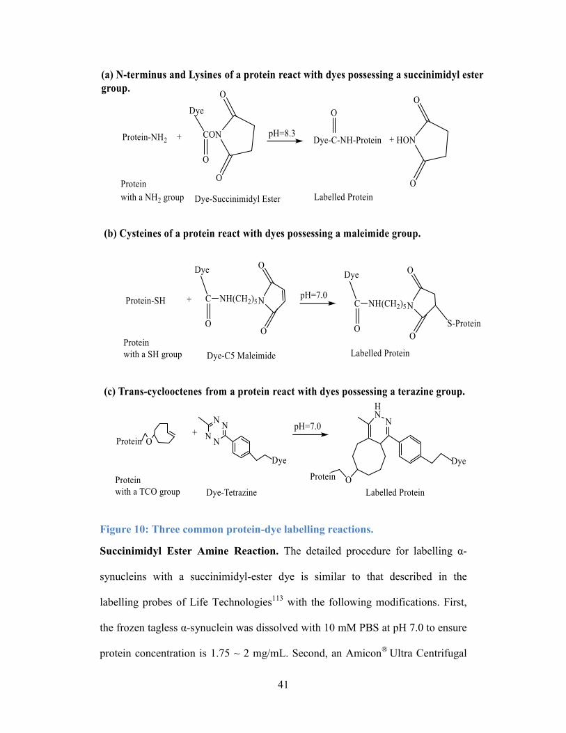
41
Figure 10: Three common protein-dye labelling reactions.
Succinimidyl Ester Amine Reaction. The detailed procedure for labelling α-
synucleins with a succinimidyl-ester dye is similar to that described in the
labelling probes of Life Technologies113
with the following modifications. First,
the frozen tagless α-synuclein was dissolved with 10 mM PBS at pH 7.0 to ensure
protein concentration is 1.75 ~ 2 mg/mL. Second, an Amicon®
Ultra Centrifugal
42
Filter with appropriate cutoff was used to remove any leftover ammonium ion and
to concentrate the protein solution to 7~8 mg/mL. Third, 0.1 mL of 1 M of sodium
bicarbonate buffer at pH 9.0 was added for each mL of protein solution. Fourth,
20 moles of the succinimidyl-ester dye were added for each mole of protein
solution. Finally, the protein-dye solution was incubated at 4 °C with continuous
stirring overnight. Because there are fifteen Lysines in the sequence of
monomeric α-synuclein, multiple dyes are theoretically able to form covalent
bonds with each monomeric α-synuclein in this method.
Sulfhydryl Maleimide Reaction. There are two ways to label the C-terminal
Cysteine of α-synucleins with dyes containing a maleimide group. The first
approach is similar to that described in the labelling probes of Life
Technologies114
with the following modifications. First, the frozen α-synuclein
with C-terminal Cysteine was dissolved with 10 mM PBS at pH 7.0 to ensure
protein concentration is 1.75 ~ 2 mg/mL. To reduce the disulfide bonds of α-
synuclein, 0.067 M of TCEP-HCl solution at pH 7.0 (TCEP-HCl solution is
titrated with NaOH solution to pH 7.0) were added into the protein solution to
ensure approximately 10-20 moles of TCEP-HCl for each mole of protein. After
45 minutes of incubation at room temperature, 20-30 moles of the maleimide dye
were added for each mole of protein. Last, the protein-dye solution was incubated
at 4 °C with continuous stirring overnight. However, according to Kim115
, large
amounts of TCEP-HCl will interfere with the sulfhydryl maleimide reaction. In
this case, the first labelling method requires large amounts of dye to compromise
the effects of interference, which complicate the purification steps.
43
To solve this problem, a second labelling approach was proposed and applied.
First of all, one modification was added in the last step of α-synuclein synthesis:
while 90% ammonia sulfate were used to precipitate the purified α-synuclein for
labelling or storage at -80 °C, 10 mM TCEP-HCl was added into the 90%
ammonia sulfate to produce the reduced solid α-synucleins. By doing this, the
unreacted excess amounts of TCEP-HCl would stay in the solution while the
protein precipitated. Moreover, the reduced solid proteins were not easily
oxidized to form disulfide bonds since movement of the solid proteins was
restricted. Next, the reduced solid α-synuclein was washed with 90% ammonia
sulfate twice to remove leftover TCEP-HCl on the surface of the solid protein.
Then, only 5~10 moles of dye solution were added for each mole of protein.
Finally, 10 mM PBS at pH 7.0 was used to dissolve the mixture of the protein and
the dye, so that the final protein concentration was around 2 mg/mL. Then, the
protein-dye solution was incubated at 4 °C with continuous stirring overnight.
To distinguish these two different sulfhydryl maleimide labelling methods, the
former one was called sulfhydryl maleimide labelling Method One and the latter
was sulfhydryl maleimide labelling Method Two.
Trans-cyclooctenes (TCO) Tetrazine Reaction. The mutated C-terminal
Cysteine α-synucleins have no TCO group. Therefore, TPM were used to
conjugate with the mutated α-synuclein based on the sulfhydryl maleimide
labelling protocol. Then, an Amicon®
Ultra Centrifugal Filter with appropriate
cutoff was used to remove excess TPM. Last, only 1~1.1 moles of the tetrazine
44
dye were added for each mole of the TPM-modified α-synuclein and the protein-
dye solution was incubated at 4 °C with continuous stirring for 4 hours.
3.2 Purification and labelling efficiency
In my research, two different approaches were applied to remove the excess dye
after labelling. They are fast protein liquid chromatography (FPLC) and
centrifugation with specific centrifugal filters. The detailed instrumentation,
materials and methods are discussed below. Then, high performance liquid
chromatography - mass spectrometry (HPLC-MS) was applied to ensure the
labelling efficiency calculation and to validate the labelling protocols based on the
sulfhydryl maleimide reaction.
3.2.1 Fast protein liquid chromatography (FPLC)
Instrumentation. All FPLC elution profiles and purified protein-dye conjugates
were obtained using an AKTA FPLC system, which consists of a AKTAmicro and
a Fraction Collector Frac-950. The AKTAmicro is a chromatography system
including a Pump P-905, a Monitor pH/C-900, and a Monitor UV-900. In
combination with two GE Healthcare HiTrap desalting columns (5mL for each),
the whole system allows me to purify at most 1.5 mL of labelled α-synuclein
solution at each sample run and to automatically collect all fraction volumes in
microliterscale. Moreover, the whole experiment process is operated by
UNICORN 5 control software. For each sample run, a FPLC chromatogram, a
plot of absorption of eluted solution vs. the elution volume, is generated.
Therefore, the fraction volume that contains purified labelled α-synucleins can be
easily determined based on their absorption and expected elution time.
45
Materials and methods. Materials of this experiment include: Two HiTrap
desalting columns (5 × 5 mL, Product Code: 71-1408-01) from GH Healthcare
Life Sciences, 20% Ethanol solution from Sigma-Aldrich, 10 mM PBS at pH =
7.4, fluorescent dye labelled α-synuclein solution (100 𝜇𝐿, protein concentration
is less than 3 mg/mL), original fluorescent dye dissolved in PBS ( ~ 3 𝜇𝑀).
Theoretically, the protein and dye concentration does not affect the FPLC
separation as long as the viscosity of total protein and dye solution is similar to
the viscosity of the PBS buffer. However, α-synuclein sample concentration used
by FPLC purification was no more than 3 mg/mL. There are two reasons: α-
synuclein aggregates quickly at high protein concentration (~ 8 mg/mL); and
excess dye and the protein are not able to be completely separated when sample
protein concentration is too high. The FPLC purification procedure is the same as
that described in the AKTA FPLC system online standard operating procedure.116
The injection volume of sample is 1 mL, flow rate of separating the protein and
dye is set at 3 mL/min and the column pressure during the separation is usually
below 0.67 MPa. Before each separation experiment, 40 mL ddH2O, and then 40
mL 1× PBS will be used to wash the column and the line. After each separation,
50 mL ddH2O are used to wash the column. Finally the column is stored at 25%
ethanol.
3.2.1 Centrions, centrifuge, and UV/Vis spectroscopy
Instrumentation and materials. The instruments used in this section were an
AllegraTM
25R Centrifuge from Beckman Coulter and an Agilent Cary 60 UV/Vis
spectrophotometer. The necessary materials are several Amicon®
Ultra
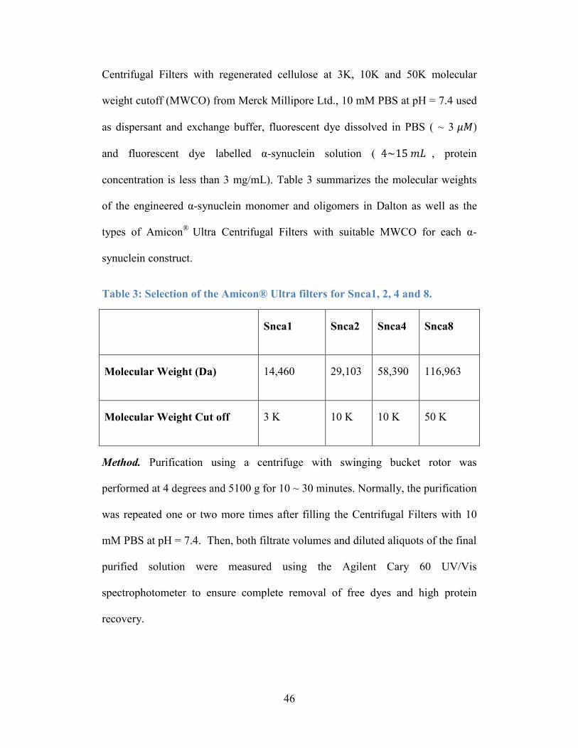
46
Centrifugal Filters with regenerated cellulose at 3K, 10K and 50K molecular
weight cutoff (MWCO) from Merck Millipore Ltd., 10 mM PBS at pH = 7.4 used
as dispersant and exchange buffer, fluorescent dye dissolved in PBS ( ~ 3 𝜇𝑀)
and fluorescent dye labelled α-synuclein solution ( 4~15 𝑚𝐿 , protein
concentration is less than 3 mg/mL). Table 3 summarizes the molecular weights
of the engineered α-synuclein monomer and oligomers in Dalton as well as the
types of Amicon®
Ultra Centrifugal Filters with suitable MWCO for each α-
synuclein construct.
Table 3: Selection of the Amicon® Ultra filters for Snca1, 2, 4 and 8.
Snca1 Snca2 Snca4 Snca8
Molecular Weight (Da) 14,460 29,103 58,390 116,963
Molecular Weight Cut off 3 K 10 K 10 K 50 K
Method. Purification using a centrifuge with swinging bucket rotor was
performed at 4 degrees and 5100 g for 10 ~ 30 minutes. Normally, the purification
was repeated one or two more times after filling the Centrifugal Filters with 10
mM PBS at pH = 7.4. Then, both filtrate volumes and diluted aliquots of the final
purified solution were measured using the Agilent Cary 60 UV/Vis
spectrophotometer to ensure complete removal of free dyes and high protein
recovery.
47
Data analysis. A good purification result with high protein recovery is
characterized by a high labelling efficiency. For instance, Alexa Fluor® 488 C5
Maleimide has its maximum absorption at 493 nm. The labelling efficiency for a
purified protein sample labelled with Alexa Fluor® 488 C5 Maleimide is defined
in Equation (27).
𝑪𝒐𝒏𝒄𝒆𝒏𝒕𝒓𝒂𝒕𝒊𝒐𝒏 𝒐𝒇 𝒅𝒚𝒆
𝑪𝒐𝒏𝒄𝒆𝒏𝒕𝒓𝒂𝒕𝒊𝒐𝒏 𝒐𝒇 𝒑𝒓𝒐𝒕𝒆𝒊𝒏=
𝑨(𝟒𝟗𝟐 𝒏𝒎)/𝜺(𝒂𝒍𝒆𝒙𝒂 𝟒𝟖𝟖)
[𝑨(𝟐𝟖𝟎 𝒏𝒎)−𝑨(𝟒𝟗𝟐 𝒏𝒎)× 𝑪𝑭]/𝜺(𝑷𝒓𝒐𝒕𝒆𝒊𝒏) (27)
where 𝐴(493 𝑛𝑚) refers to the absorption at wavelength 493 nm, 휀(𝐴𝑙𝑒𝑥𝑎 488)
is the molar absorptivity of Alexa Fluor®
488 C5 Maleimide ( 7.0000 ×
104 𝑀−1𝑐𝑚−1) and CF is the correction factor113
, which is equal to 𝐴(280 𝑛𝑚)
𝐴(493 𝑛𝑚) of a
sample only contained Alexa Fluor® 488 C5 Maleimide. Normally, CF of a
specific dye was given by the manufacturer, for example, CF of that Alexa Fluor®
488 C5 Maleimide is 0.11, CF of Oregon Green 488 maleimide is 0.12 and CF of
Cy5 tetrazine is 0.08.
3.2.3 HPLC-ESI-oaTOF
High performance liquid chromatography with an orthogonal acceleration time-
of-flight mass spectrometer (HPLC-ESI-oaTOF) was used: (i) as an innovative
method to confirm the calculation of the labelling efficiency; and (ii) to ensure a
successful labelling between TPM and α-synuclein.
Instrumentation. The instruments used in this section were Agilent 1200 SL
HPLC system and an oaTOF mass spectrometer. Electrospray ionization (ESI)
was used to generate the ion source for the oaTOF mass spectrometer. A 75×0.5
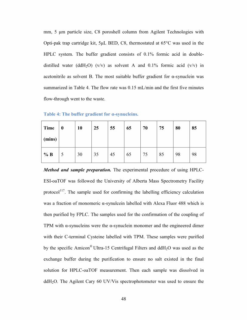
48
mm, 5 μm particle size, C8 poroshell column from Agilent Technologies with
Opti-pak trap cartridge kit, 5μL BED, C8, thermostated at 65°C was used in the
HPLC system. The buffer gradient consists of 0.1% formic acid in double-
distilled water (ddH2O) (v/v) as solvent A and 0.1% formic acid (v/v) in
acetonitrile as solvent B. The most suitable buffer gradient for α-synuclein was
summarized in Table 4. The flow rate was 0.15 mL/min and the first five minutes
flow-through went to the waste.
Table 4: The buffer gradient for α-synucleins.
Time
(mins)
0 10 25 55 65 70 75 80 85
% B 5 30 35 45 65 75 85 98 98
Method and sample preparation. The experimental procedure of using HPLC-
ESI-oaTOF was followed the University of Alberta Mass Spectrometry Facility
protocol117
. The sample used for confirming the labelling efficiency calculation
was a fraction of monomeric α-synulcein labelled with Alexa Fluor 488 which is
then purified by FPLC. The samples used for the confirmation of the coupling of
TPM with α-synucleins were the α-synuclein monomer and the engineered dimer
with their C-terminal Cysteine labelled with TPM. These samples were purified
by the specific Amicon®
Ultra-15 Centrifugal Filters and ddH2O was used as the
exchange buffer during the purification to ensure no salt existed in the final
solution for HPLC-oaTOF measurement. Then each sample was dissolved in
ddH2O. The Agilent Cary 60 UV/Vis spectrophotometer was used to ensure the
49
protein concentration was approximately 30 μM. Then 2 µL of the sample was
diluted with 12 μL of 0.1% formic acid in (ddH2O) (v/v), and 2 μL of the diluted
sample was injected.
3.3 Quantum yields of labelled α-synucleins
This experiment aimed to find out whether the quantum yield of Oregon Green
488 Maleimide or Cy5 tetrazine changed or not when they were mixed with or
were conjugated to the monomeric, dimeric, tetrameric and octameric α-
synucleins.
Instrumentation. The instrument used in this section was a PTI Fluorescence
QuantaMasterTM
Fluorescence Spectrofluorometer. The accompanying software
was FelixGX 4.1.2. A wavelength of 492 nm was used to excite Oregon Green
488 Maleimide and its labelled protein. The fluorescence of the dye from 493 nm
to 600 nm was detected at 90°. Similarly, a wavelength of 650 nm was used to
excite Cy5 tetrazine and its labelled protein, the fluorescence of the dye from 651
nm to 750 nm was detected at 90°. For all measurements, the entrance and exits
sides of both the excitation and emission monochromators were set to 1 nm. A
clean, 1 cm, quartz cuvette was used.
Method and sample preparation. The α-synuclein monomer, dimer, tetramer and
octamer with their C-terminal Cysteine labelled with either Oregon Green 488
maleimide or Cy5 tetrazine, together with the pure dyes and 10 mM PBS buffer
were measured using the PTI Fluorescence Spectrofluorometer. Each sample was
dissolved in the 10 mM PBS at pH 7.4 and the protein concentration was
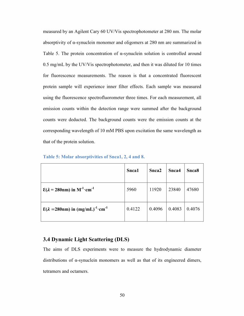
50
measured by an Agilent Cary 60 UV/Vis spectrophotometer at 280 nm. The molar
absorptivity of α-synuclein monomer and oligomers at 280 nm are summarized in
Table 5. The protein concentration of α-synuclein solution is controlled around
0.5 mg/mL by the UV/Vis spectrophotometer, and then it was diluted for 10 times
for fluorescence measurements. The reason is that a concentrated fluorescent
protein sample will experience inner filter effects. Each sample was measured
using the fluorescence spectrofluorometer three times. For each measurement, all
emission counts within the detection range were summed after the background
counts were deducted. The background counts were the emission counts at the
corresponding wavelength of 10 mM PBS upon excitation the same wavelength as
that of the protein solution.
Table 5: Molar absorptivities of Snca1, 2, 4 and 8.
Snca1 Snca2 Snca4 Snca8
Ɛ(𝝀 = 280nm) in M-1
·cm-1
5960 11920 23840 47680
Ɛ(𝝀 =280nm) in (mg/mL)-1
·cm-1
0.4122 0.4096 0.4083 0.4076
3.4 Dynamic Light Scattering (DLS)
The aims of DLS experiments were to measure the hydrodynamic diameter
distributions of α-synuclein monomers as well as that of its engineered dimers,
tetramers and octamers.

51
Instrumentation and method. The instrument used in this experiment was a
Zetasizer Nano ZS. It used an excitation wavelength of 633 nm and detected the
scattering light at 173°. The accompanied software for the Zetasizer Nano ZS is
Malvern Software (version 7.02). For all measurements, the suggested Standard
Operating Procedures (SOP) was used. The SOP includes that the refractive index
and the absorption of the measured protein were set at 1.450 and 0.001,
respectively, 10 mM PBS was used as dispersant, and its viscosity and refractive
index at the measurement temperature (22.0 °C) were set at 1.05 cP and 1.334,
respectively. Disposable DTS0012 cuvettes were used. To improve the signal-to-
noise ratio, each sample was measured three times and each measurement
contained 13 runs.
Sample Preparation. The α-synuclein monomer, dimer, tetramer and octamer
with their C-terminal Cysteine labelled with TPM were measured by DLS. Each
sample was dissolved in 10 mM PBS at pH 7.4 and with a protein concentration
of approximately 1.4 mg/mL. An Agilent Cary 60 UV/Vis spectrophotometer was
used to measure the protein concentration at 280 nm. To remove dust and large
protein aggregates, Whatman Anotop 10 Syringe Filters with 100 nm pore size
were used to filter 1.5 mL of each protein sample directly into new disposable
DTS0012 cuvettes for measurements.
3.5 FCS and dual-color FCCS
3.5.1 Calibration measurements
Laser-scanning microscope LSM 510/ConfoCor 2 (CarlZeiss, Jena, Germany)
was used for all FCS measurements and a C-Apochromat 40X/NA 1.2 water
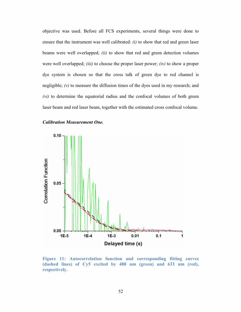
52
objective was used. Before all FCS experiments, several things were done to
ensure that the instrument was well calibrated: (i) to show that red and green laser
beams were well overlapped; (ii) to show that red and green detection volumes
were well overlapped; (iii) to choose the proper laser power; (iv) to show a proper
dye system is chosen so that the cross talk of green dye to red channel is
negligible; (v) to measure the diffusion times of the dyes used in my research; and
(vi) to determine the equatorial radius and the confocal volumes of both green
laser beam and red laser beam, together with the estimated cross confocal volume.
Calibration Measurement One.
Figure 11: Autocorrelation function and corresponding fitting curves
(dashed lines) of Cy5 excited by 488 nm (green) and 633 nm (red),
respectively.
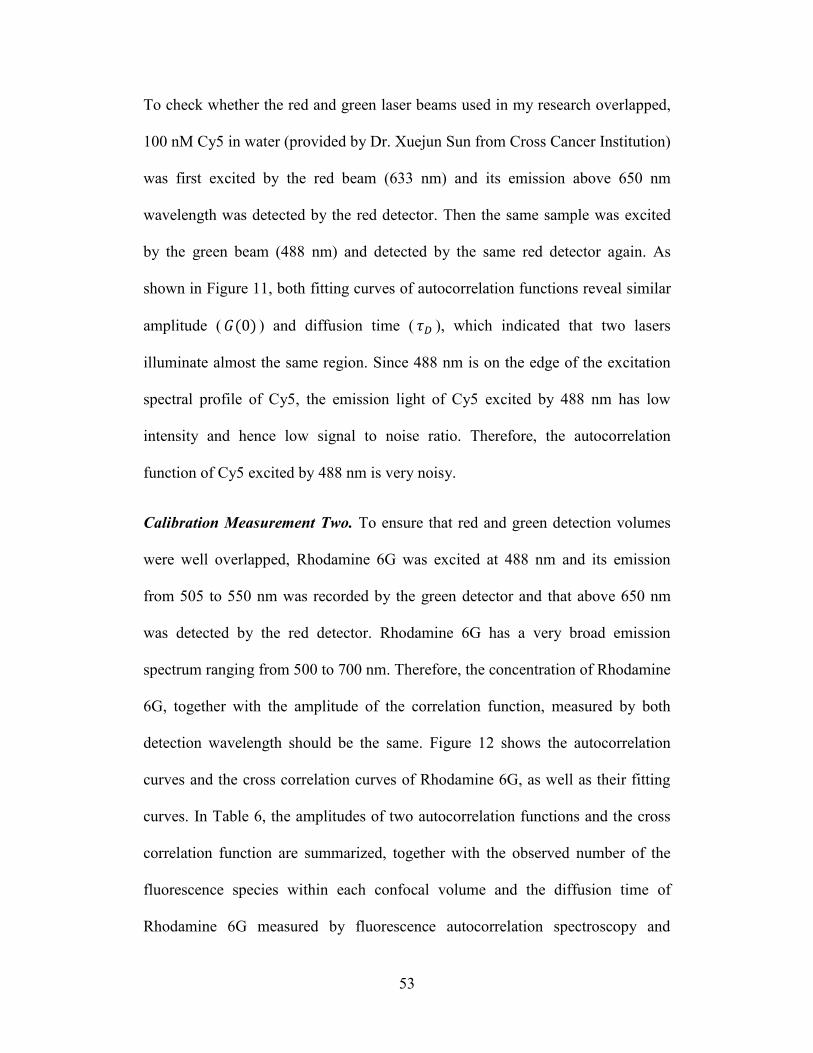
53
To check whether the red and green laser beams used in my research overlapped,
100 nM Cy5 in water (provided by Dr. Xuejun Sun from Cross Cancer Institution)
was first excited by the red beam (633 nm) and its emission above 650 nm
wavelength was detected by the red detector. Then the same sample was excited
by the green beam (488 nm) and detected by the same red detector again. As
shown in Figure 11, both fitting curves of autocorrelation functions reveal similar
amplitude ( 𝐺(0) ) and diffusion time ( 𝜏𝐷 ), which indicated that two lasers
illuminate almost the same region. Since 488 nm is on the edge of the excitation
spectral profile of Cy5, the emission light of Cy5 excited by 488 nm has low
intensity and hence low signal to noise ratio. Therefore, the autocorrelation
function of Cy5 excited by 488 nm is very noisy.
Calibration Measurement Two. To ensure that red and green detection volumes
were well overlapped, Rhodamine 6G was excited at 488 nm and its emission
from 505 to 550 nm was recorded by the green detector and that above 650 nm
was detected by the red detector. Rhodamine 6G has a very broad emission
spectrum ranging from 500 to 700 nm. Therefore, the concentration of Rhodamine
6G, together with the amplitude of the correlation function, measured by both
detection wavelength should be the same. Figure 12 shows the autocorrelation
curves and the cross correlation curves of Rhodamine 6G, as well as their fitting
curves. In Table 6, the amplitudes of two autocorrelation functions and the cross
correlation function are summarized, together with the observed number of the
fluorescence species within each confocal volume and the diffusion time of
Rhodamine 6G measured by fluorescence autocorrelation spectroscopy and
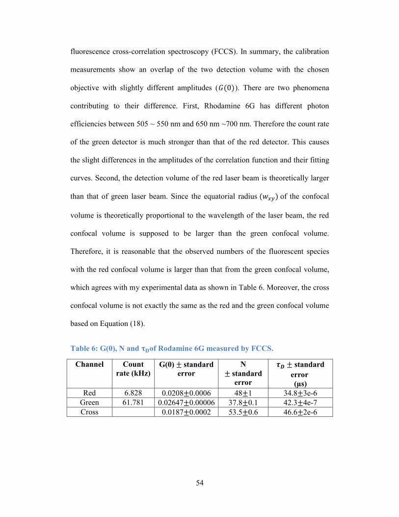
54
fluorescence cross-correlation spectroscopy (FCCS). In summary, the calibration
measurements show an overlap of the two detection volume with the chosen
objective with slightly different amplitudes (𝐺(0)). There are two phenomena
contributing to their difference. First, Rhodamine 6G has different photon
efficiencies between 505 ~ 550 nm and 650 nm ~700 nm. Therefore the count rate
of the green detector is much stronger than that of the red detector. This causes
the slight differences in the amplitudes of the correlation function and their fitting
curves. Second, the detection volume of the red laser beam is theoretically larger
than that of green laser beam. Since the equatorial radius (𝑤𝑥𝑦) of the confocal
volume is theoretically proportional to the wavelength of the laser beam, the red
confocal volume is supposed to be larger than the green confocal volume.
Therefore, it is reasonable that the observed numbers of the fluorescent species
with the red confocal volume is larger than that from the green confocal volume,
which agrees with my experimental data as shown in Table 6. Moreover, the cross
confocal volume is not exactly the same as the red and the green confocal volume
based on Equation (18).
Table 6: G(0), N and 𝛕𝐃of Rodamine 6G measured by FCCS.
Channel
Count
rate (kHz)
G(0) ± standard
error
N
± standard
error
𝝉𝑫 ± standard
error (µs)
Red 6.828 0.0208±0.0006 48±1 34.8±3e-6
Green 61.781 0.02647±0.00006 37.8±0.1 42.3±4e-7
Cross 0.0187±0.0002 53.5±0.6 46.6±2e-6
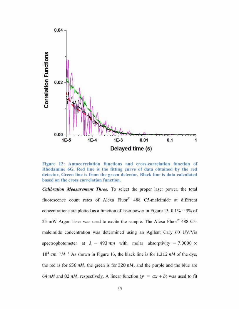
55
Figure 12: Autocorrelation functions and cross-correlation function of
Rhodamine 6G. Red line is the fitting curve of data obtained by the red
detector, Green line is from the green detector, Black line is data calculated
based on the cross correlation function.
Calibration Measurement Three. To select the proper laser power, the total
fluorescence count rates of Alexa Fluor®
488 C5-maleimide at different
concentrations are plotted as a function of laser power in Figure 13. 0.1% ~ 3% of
25 mW Argon laser was used to excite the sample. The Alexa Fluor® 488 C5-
maleimide concentration was determined using an Agilent Cary 60 UV/Vis
spectrophotometer at 𝜆 = 493 𝑛𝑚 with molar absorptivity = 7.0000 ×
104 𝑐𝑚−1𝑀−1 As shown in Figure 13, the black line is for 1.312 𝑛𝑀 of the dye,
the red is for 656 𝑛𝑀, the green is for 328 𝑛𝑀, and the purple and the blue are
64 𝑛𝑀 and 82 𝑛𝑀, respectively. A linear function (𝑦 = 𝑎𝑥 + 𝑏) was used to fit
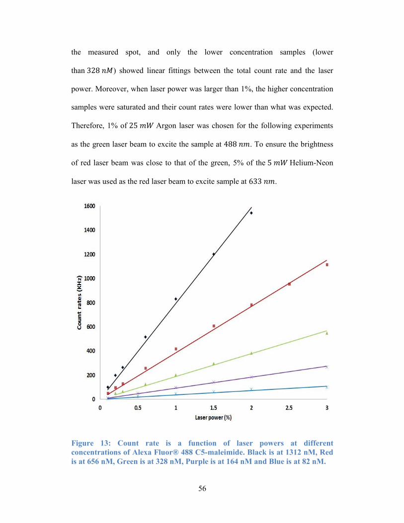
56
the measured spot, and only the lower concentration samples (lower
than 328 𝑛𝑀) showed linear fittings between the total count rate and the laser
power. Moreover, when laser power was larger than 1%, the higher concentration
samples were saturated and their count rates were lower than what was expected.
Therefore, 1% of 25 𝑚𝑊 Argon laser was chosen for the following experiments
as the green laser beam to excite the sample at 488 𝑛𝑚. To ensure the brightness
of red laser beam was close to that of the green, 5% of the 5 𝑚𝑊 Helium-Neon
laser was used as the red laser beam to excite sample at 633 𝑛𝑚.
Figure 13: Count rate is a function of laser powers at different
concentrations of Alexa Fluor® 488 C5-maleimide. Black is at 1312 nM, Red
is at 656 nM, Green is at 328 nM, Purple is at 164 nM and Blue is at 82 nM.
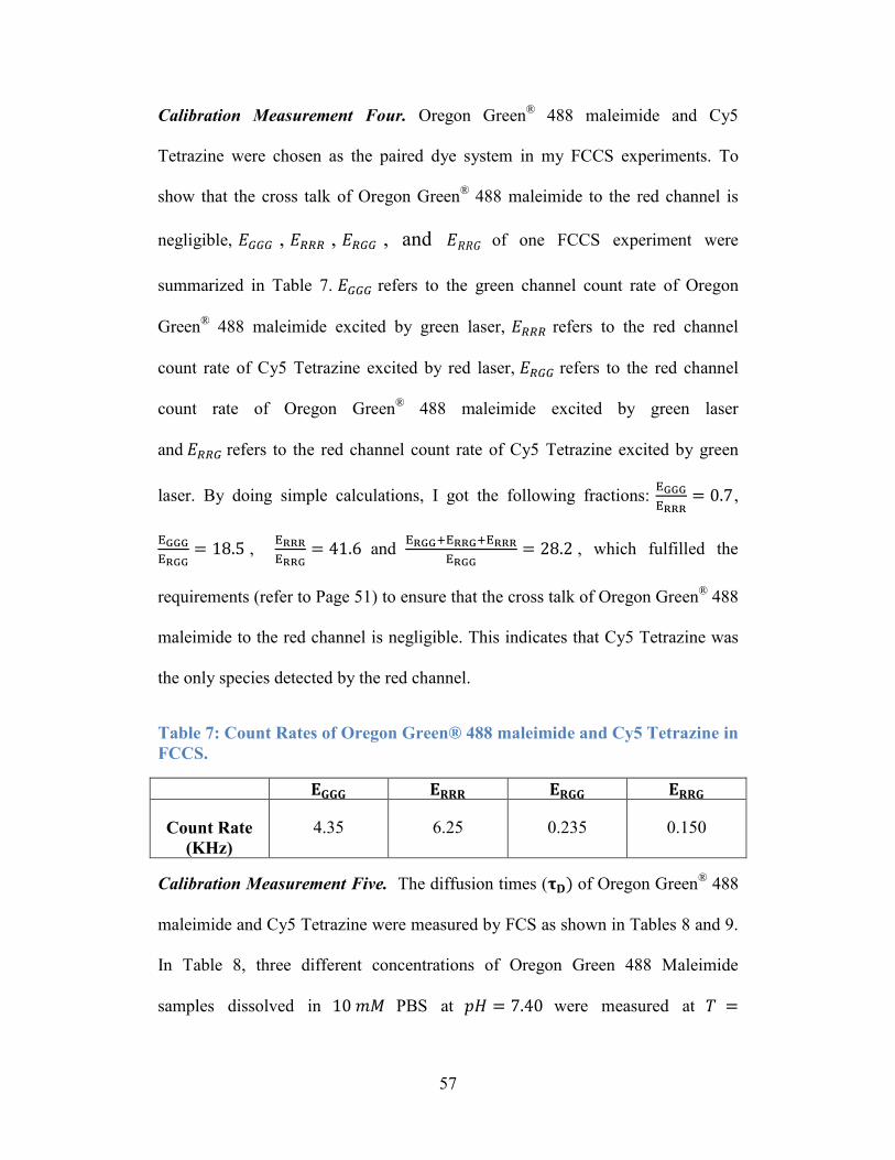
57
Calibration Measurement Four. Oregon Green® 488 maleimide and Cy5
Tetrazine were chosen as the paired dye system in my FCCS experiments. To
show that the cross talk of Oregon Green® 488 maleimide to the red channel is
negligible, 𝐸𝐺𝐺𝐺 , 𝐸𝑅𝑅𝑅 , 𝐸𝑅𝐺𝐺 , and 𝐸𝑅𝑅𝐺 of one FCCS experiment were
summarized in Table 7. 𝐸𝐺𝐺𝐺 refers to the green channel count rate of Oregon
Green® 488 maleimide excited by green laser, 𝐸𝑅𝑅𝑅 refers to the red channel
count rate of Cy5 Tetrazine excited by red laser, 𝐸𝑅𝐺𝐺 refers to the red channel
count rate of Oregon Green® 488 maleimide excited by green laser
and 𝐸𝑅𝑅𝐺 refers to the red channel count rate of Cy5 Tetrazine excited by green
laser. By doing simple calculations, I got the following fractions: EGGG
ERRR= 0.7,
EGGG
ERGG= 18.5 ,
ERRR
ERRG= 41.6 and
ERGG+ERRG+ERRR
ERGG= 28.2 , which fulfilled the
requirements (refer to Page 51) to ensure that the cross talk of Oregon Green® 488
maleimide to the red channel is negligible. This indicates that Cy5 Tetrazine was
the only species detected by the red channel.
Table 7: Count Rates of Oregon Green® 488 maleimide and Cy5 Tetrazine in
FCCS.
𝐄𝐆𝐆𝐆 𝐄𝐑𝐑𝐑 𝐄𝐑𝐆𝐆 𝐄𝐑𝐑𝐆
Count Rate
(KHz)
4.35 6.25 0.235 0.150
Calibration Measurement Five. The diffusion times (𝛕𝐃) of Oregon Green® 488
maleimide and Cy5 Tetrazine were measured by FCS as shown in Tables 8 and 9.
In Table 8, three different concentrations of Oregon Green 488 Maleimide
samples dissolved in 10 𝑚𝑀 PBS at 𝑝𝐻 = 7.40 were measured at 𝑇 =
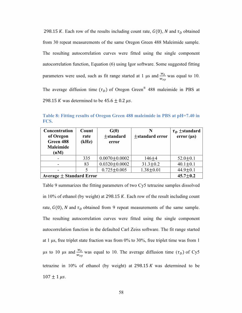
58
298.15 𝐾. Each row of the results including count rate, 𝐺(0), 𝑁 and 𝜏𝐷 obtained
from 30 repeat measurements of the same Oregon Green 488 Maleimide sample.
The resulting autocorrelation curves were fitted using the single component
autocorrelation function, Equation (6) using Igor software. Some suggested fitting
parameters were used, such as fit range started at 1 μs and 𝑤𝑧
𝑤𝑥𝑦 was equal to 10.
The average diffusion time (𝜏𝐷) of Oregon Green®
488 maleimide in PBS at
298.15 𝐾 was determined to be 45.6 ± 0.2 𝜇𝑠.
Table 8: Fitting results of Oregon Green 488 maleimide in PBS at pH=7.40 in
FCS.
Concentration
of Oregon
Green 488
Maleimide
(nM)
Count
rate
(kHz)
G(0)
±standard
error
N
±standard error
𝝉𝑫 ±standard
error (µs)
- 335 0.0070±0.0002 146±4 52.0±0.1
- 83 0.0320±0.0002 31.3±0.2 40.1±0.1
- 5 0.725±0.005 1.38±0.01 44.9±0.1
Average ± Standard Error 45.7±0.2
Table 9 summarizes the fitting parameters of two Cy5 tetrazine samples dissolved
in 10% of ethanol (by weight) at 298.15 𝐾. Each row of the result including count
rate, 𝐺(0), 𝑁 and 𝜏𝐷 obtained from 9 repeat measurements of the same sample.
The resulting autocorrelation curves were fitted using the single component
autocorrelation function in the defaulted Carl Zeiss software. The fit range started
at 1 μs, free triplet state fraction was from 0% to 30%, free triplet time was from 1
µs to 10 μs and 𝑤𝑧
𝑤𝑥𝑦 was equal to 10. The average diffusion time (𝜏𝐷) of Cy5
tetrazine in 10% of ethanol (by weight) at 298.15 𝐾 was determined to be
107 ± 1 𝜇𝑠.
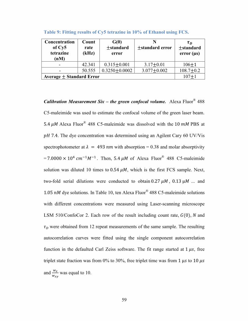
59
Table 9: Fitting results of Cy5 tetrazine in 10% of Ethanol using FCS.
Concentration
of Cy5
tetrazine
(nM)
Count
rate
(kHz)
G(0)
±standard
error
N
±standard error
𝝉𝑫
±standard
error (µs)
- 42.341 0.315±0.001 3.17±0.01 106±1
- 50.555 0.3250±0.0002 3.077±0.002 108.7±0.2
Average ± Standard Error 107±1
Calibration Measurement Six – the green confocal volume. Alexa Fluor® 488
C5-maleimide was used to estimate the confocal volume of the green laser beam.
5.4 𝜇𝑀 Alexa Fluor® 488 C5-maleimide was dissolved with the 10 𝑚𝑀 PBS at
𝑝𝐻 7.4. The dye concentration was determined using an Agilent Cary 60 UV/Vis
spectrophotometer at 𝜆 = 493 𝑛𝑚 with absorption = 0.38 and molar absorptivity
= 7.0000 × 10⁴ 𝑐𝑚−1𝑀−1 . Then, 5.4 𝜇𝑀 of Alexa Fluor® 488 C5-maleimide
solution was diluted 10 times to 0.54 𝜇𝑀, which is the first FCS sample. Next,
two-fold serial dilutions were conducted to obtain 0.27 𝜇𝑀 , 0.13 μ𝑀 ... and
1.05 𝑛𝑀 dye solutions. In Table 10, ten Alexa Fluor® 488 C5-maleimide solutions
with different concentrations were measured using Laser-scanning microscope
LSM 510/ConfoCor 2. Each row of the result including count rate, 𝐺(0), 𝑁 and
𝜏𝐷 were obtained from 12 repeat measurements of the same sample. The resulting
autocorrelation curves were fitted using the single component autocorrelation
function in the defaulted Carl Zeiss software. The fit range started at 1 𝜇𝑠, free
triplet state fraction was from 0% to 30%, free triplet time was from 1 μ𝑠 to 10 𝜇𝑠
and 𝑤𝑧
𝑤𝑥𝑦 was equal to 10.
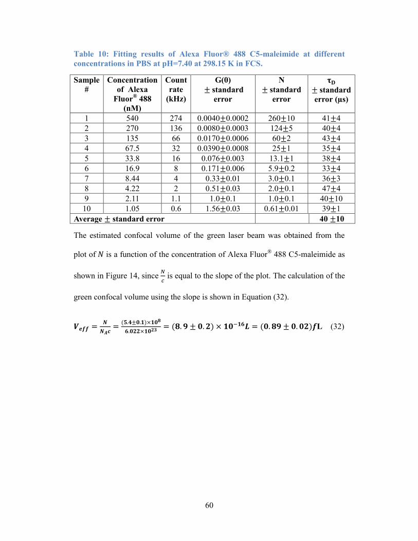
60
Table 10: Fitting results of Alexa Fluor® 488 C5-maleimide at different
concentrations in PBS at pH=7.40 at 298.15 K in FCS.
Sample
#
Concentration
of Alexa
Fluor®
488
(nM)
Count
rate
(kHz)
G(0)
± standard
error
N
± standard
error
𝛕𝐃
± standard
error (µs)
1 540 274 0.0040±0.0002 260±10 41±4
2 270 136 0.0080±0.0003 124±5 40±4
3 135 66 0.0170±0.0006 60±2 43±4
4 67.5 32 0.0390±0.0008 25±1 35±4
5 33.8 16 0.076±0.003 13.1±1 38±4
6 16.9 8 0.171±0.006 5.9±0.2 33±4
7 8.44 4 0.33±0.01 3.0±0.1 36±3
8 4.22 2 0.51±0.03 2.0±0.1 47±4
9 2.11 1.1 1.0±0.1 1.0±0.1 40±10
10 1.05 0.6 1.56±0.03 0.61±0.01 39±1
Average ± standard error 40 ±10
The estimated confocal volume of the green laser beam was obtained from the
plot of 𝑁 is a function of the concentration of Alexa Fluor® 488 C5-maleimide as
shown in Figure 14, since 𝑁
𝑐 is equal to the slope of the plot. The calculation of the
green confocal volume using the slope is shown in Equation (32).
𝑽𝒆𝒇𝒇 =𝑵
𝑵𝑨𝒄=
(𝟓.𝟒±𝟎.𝟏)×𝟏𝟎𝟖
𝟔.𝟎𝟐𝟐×𝟏𝟎𝟐𝟑 = (𝟖. 𝟗 ± 𝟎. 𝟐) × 𝟏𝟎−𝟏𝟔𝑳 = (𝟎. 𝟖𝟗 ± 𝟎. 𝟎𝟐)𝒇L (32)
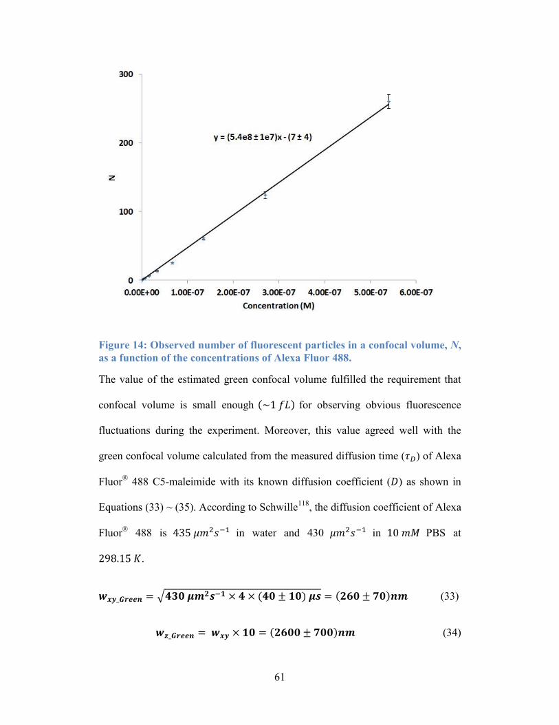
61
Figure 14: Observed number of fluorescent particles in a confocal volume, N,
as a function of the concentrations of Alexa Fluor 488.
The value of the estimated green confocal volume fulfilled the requirement that
confocal volume is small enough (~1 𝑓𝐿) for observing obvious fluorescence
fluctuations during the experiment. Moreover, this value agreed well with the
green confocal volume calculated from the measured diffusion time (𝜏𝐷) of Alexa
Fluor®
488 C5-maleimide with its known diffusion coefficient (𝐷) as shown in
Equations (33) ~ (35). According to Schwille118
, the diffusion coefficient of Alexa
Fluor®
488 is 435 𝜇𝑚2𝑠−1 in water and 430 𝜇𝑚2𝑠−1 in 10 𝑚𝑀 PBS at
298.15 𝐾.
𝒘𝒙𝒚_𝑮𝒓𝒆𝒆𝒏 = √𝟒𝟑𝟎 𝝁𝒎𝟐𝒔−𝟏 × 𝟒 × (𝟒𝟎 ± 𝟏𝟎) 𝝁𝒔 = (𝟐𝟔𝟎 ± 𝟕𝟎)𝒏𝒎 (33)
𝒘𝒛_𝑮𝒓𝒆𝒆𝒏 = 𝒘𝒙𝒚 × 𝟏𝟎 = (𝟐𝟔𝟎𝟎 ± 𝟕𝟎𝟎)𝒏𝒎 (34)
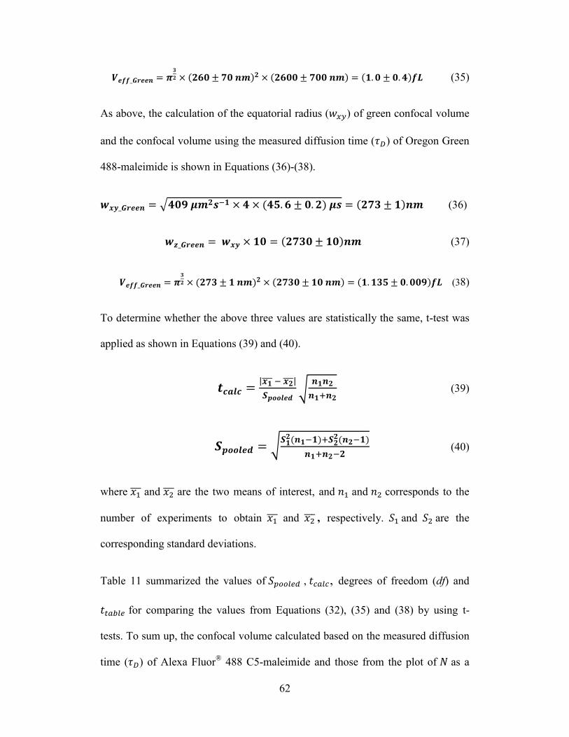
62
𝑽𝒆𝒇𝒇_𝑮𝒓𝒆𝒆𝒏 = 𝝅𝟑
𝟐 × (𝟐𝟔𝟎 ± 𝟕𝟎 𝒏𝒎)𝟐 × (𝟐𝟔𝟎𝟎 ± 𝟕𝟎𝟎 𝒏𝒎) = (𝟏. 𝟎 ± 𝟎. 𝟒)𝒇𝑳 (35)
As above, the calculation of the equatorial radius (𝑤𝑥𝑦) of green confocal volume
and the confocal volume using the measured diffusion time (𝜏𝐷) of Oregon Green
488-maleimide is shown in Equations (36)-(38).
𝒘𝒙𝒚_𝑮𝒓𝒆𝒆𝒏 = √𝟒𝟎𝟗 𝝁𝒎𝟐𝒔−𝟏 × 𝟒 × (𝟒𝟓. 𝟔 ± 𝟎. 𝟐) 𝝁𝒔 = (𝟐𝟕𝟑 ± 𝟏)𝒏𝒎 (36)
𝒘𝒛_𝑮𝒓𝒆𝒆𝒏 = 𝒘𝒙𝒚 × 𝟏𝟎 = (𝟐𝟕𝟑𝟎 ± 𝟏𝟎)𝒏𝒎 (37)
𝑽𝒆𝒇𝒇_𝑮𝒓𝒆𝒆𝒏 = 𝝅𝟑
𝟐 × (𝟐𝟕𝟑 ± 𝟏 𝒏𝒎)𝟐 × (𝟐𝟕𝟑𝟎 ± 𝟏𝟎 𝒏𝒎) = (𝟏. 𝟏𝟑𝟓 ± 𝟎. 𝟎𝟎𝟗)𝒇𝑳 (38)
To determine whether the above three values are statistically the same, t-test was
applied as shown in Equations (39) and (40).
𝒕𝒄𝒂𝒍𝒄 =|𝒙𝟏 − 𝒙𝟐 |
𝑺𝒑𝒐𝒐𝒍𝒆𝒅√
𝒏𝟏𝒏𝟐
𝒏𝟏+𝒏𝟐 (39)
𝑺𝒑𝒐𝒐𝒍𝒆𝒅 = √𝑺𝟏
𝟐(𝒏𝟏−𝟏)+𝑺𝟐𝟐(𝒏𝟐−𝟏)
𝒏𝟏+𝒏𝟐−𝟐 (40)
where 𝑥1 and 𝑥2 are the two means of interest, and 𝑛1 and 𝑛2 corresponds to the
number of experiments to obtain 𝑥1 and 𝑥2 , respectively. 𝑆1 and 𝑆2 are the
corresponding standard deviations.
Table 11 summarized the values of 𝑆𝑝𝑜𝑜𝑙𝑒𝑑 , 𝑡𝑐𝑎𝑙𝑐, degrees of freedom (df) and
𝑡𝑡𝑎𝑏𝑙𝑒 for comparing the values from Equations (32), (35) and (38) by using t-
tests. To sum up, the confocal volume calculated based on the measured diffusion
time (𝜏𝐷) of Alexa Fluor® 488 C5-maleimide and those from the plot of 𝑁 as a
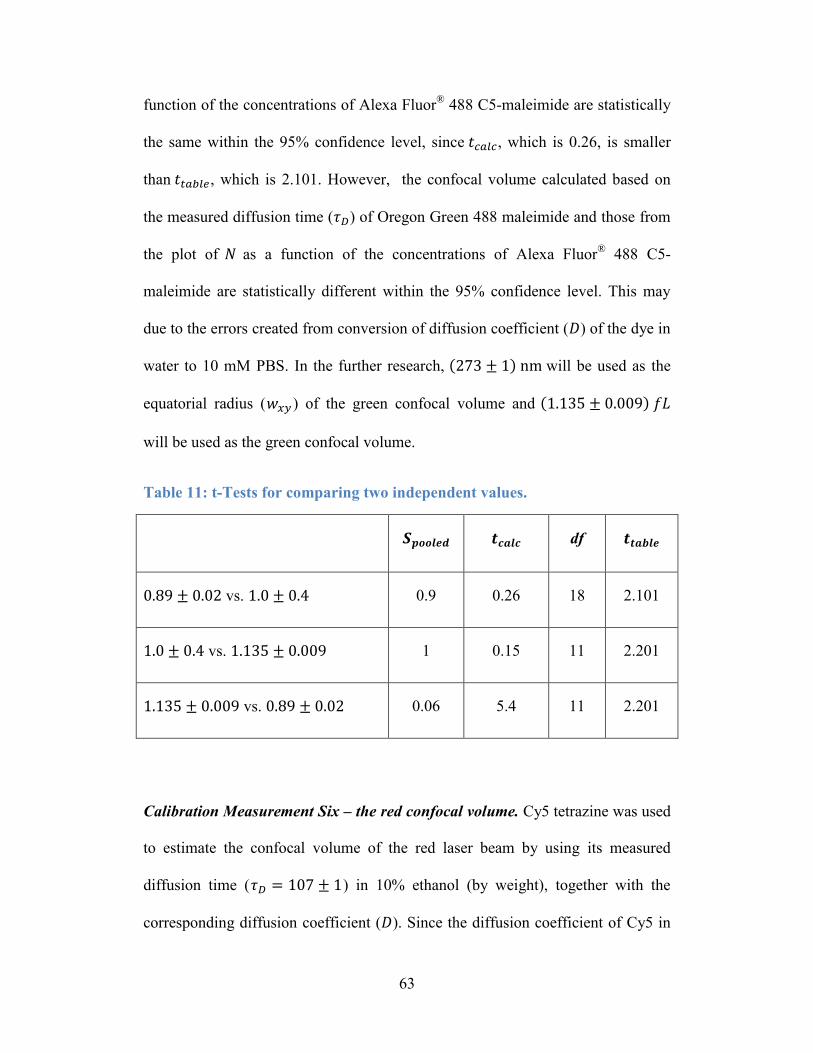
63
function of the concentrations of Alexa Fluor®
488 C5-maleimide are statistically
the same within the 95% confidence level, since 𝑡𝑐𝑎𝑙𝑐, which is 0.26, is smaller
than 𝑡𝑡𝑎𝑏𝑙𝑒, which is 2.101. However, the confocal volume calculated based on
the measured diffusion time (𝜏𝐷) of Oregon Green 488 maleimide and those from
the plot of 𝑁 as a function of the concentrations of Alexa Fluor® 488 C5-
maleimide are statistically different within the 95% confidence level. This may
due to the errors created from conversion of diffusion coefficient (𝐷) of the dye in
water to 10 mM PBS. In the further research, (273 ± 1) nm will be used as the
equatorial radius (𝑤𝑥𝑦 ) of the green confocal volume and (1.135 ± 0.009) 𝑓𝐿
will be used as the green confocal volume.
Table 11: t-Tests for comparing two independent values.
𝑺𝒑𝒐𝒐𝒍𝒆𝒅 𝒕𝒄𝒂𝒍𝒄 df 𝒕𝒕𝒂𝒃𝒍𝒆
0.89 ± 0.02 vs. 1.0 ± 0.4 0.9 0.26 18 2.101
1.0 ± 0.4 vs. 1.135 ± 0.009 1 0.15 11 2.201
1.135 ± 0.009 vs. 0.89 ± 0.02 0.06 5.4 11 2.201
Calibration Measurement Six – the red confocal volume. Cy5 tetrazine was used
to estimate the confocal volume of the red laser beam by using its measured
diffusion time (𝜏𝐷 = 107 ± 1) in 10% ethanol (by weight), together with the
corresponding diffusion coefficient (𝐷). Since the diffusion coefficient of Cy5 in
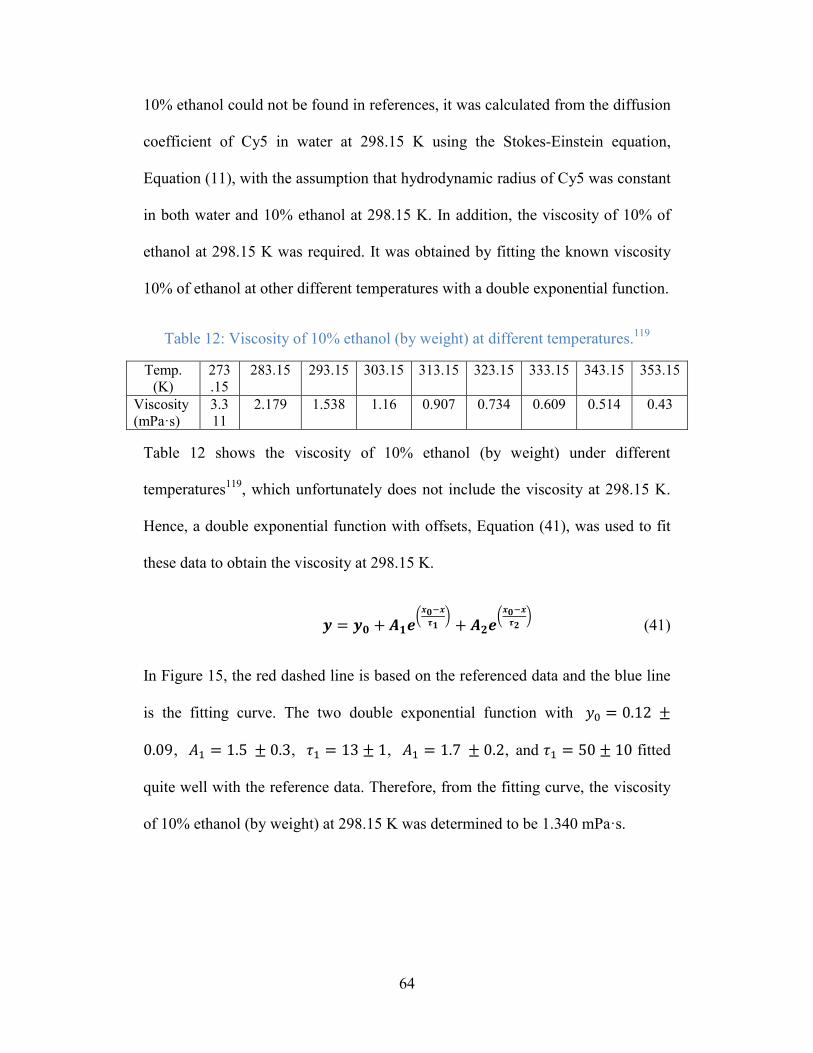
64
10% ethanol could not be found in references, it was calculated from the diffusion
coefficient of Cy5 in water at 298.15 K using the Stokes-Einstein equation,
Equation (11), with the assumption that hydrodynamic radius of Cy5 was constant
in both water and 10% ethanol at 298.15 K. In addition, the viscosity of 10% of
ethanol at 298.15 K was required. It was obtained by fitting the known viscosity
10% of ethanol at other different temperatures with a double exponential function.
Table 12: Viscosity of 10% ethanol (by weight) at different temperatures.119
Temp.
(K)
273
.15
283.15 293.15 303.15 313.15 323.15 333.15 343.15 353.15
Viscosity
(mPa·s)
3.3
11
2.179 1.538 1.16 0.907 0.734 0.609 0.514 0.43
Table 12 shows the viscosity of 10% ethanol (by weight) under different
temperatures119
, which unfortunately does not include the viscosity at 298.15 K.
Hence, a double exponential function with offsets, Equation (41), was used to fit
these data to obtain the viscosity at 298.15 K.
𝒚 = 𝒚𝟎 + 𝑨𝟏𝒆(
𝒙𝟎−𝒙
𝝉𝟏)
+ 𝑨𝟐𝒆(
𝒙𝟎−𝒙
𝝉𝟐) (41)
In Figure 15, the red dashed line is based on the referenced data and the blue line
is the fitting curve. The two double exponential function with 𝑦0 = 0.12 ±
0.09, 𝐴1 = 1.5 ± 0.3, 𝜏1 = 13 ± 1, 𝐴1 = 1.7 ± 0.2, and 𝜏1 = 50 ± 10 fitted
quite well with the reference data. Therefore, from the fitting curve, the viscosity
of 10% ethanol (by weight) at 298.15 K was determined to be 1.340 mPa·s.
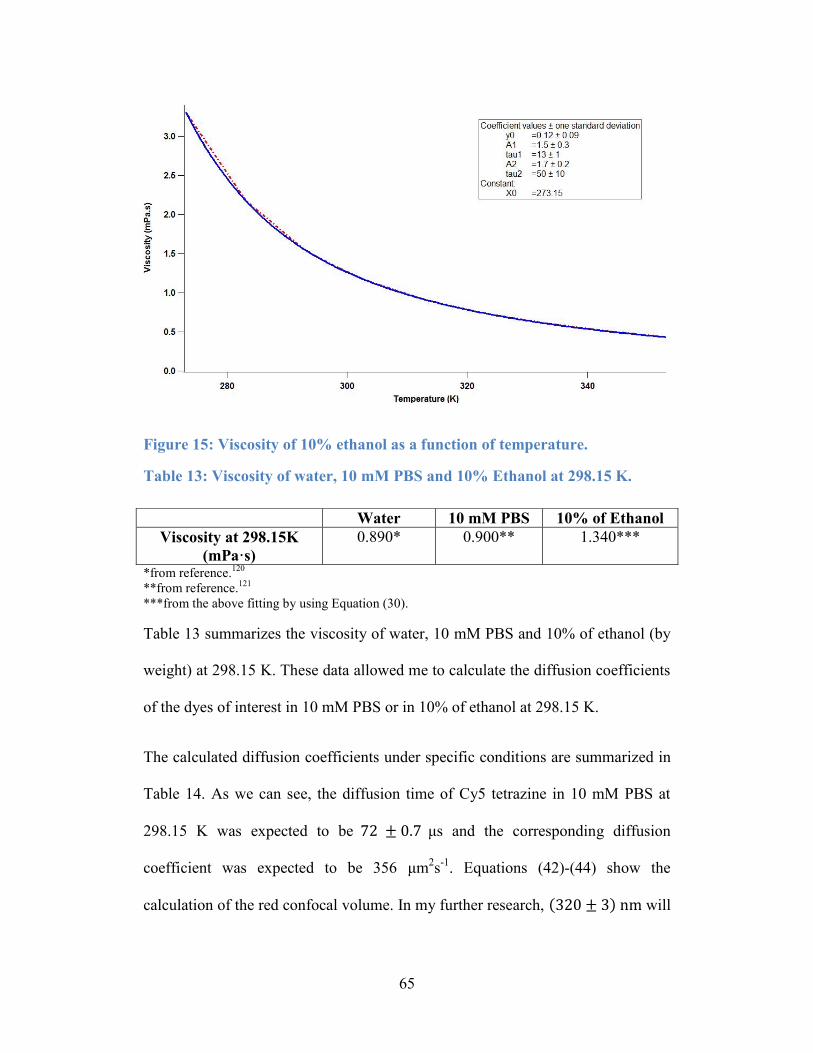
65
Figure 15: Viscosity of 10% ethanol as a function of temperature.
Table 13: Viscosity of water, 10 mM PBS and 10% Ethanol at 298.15 K.
*from reference.120
**from reference.121
***from the above fitting by using Equation (30).
Table 13 summarizes the viscosity of water, 10 mM PBS and 10% of ethanol (by
weight) at 298.15 K. These data allowed me to calculate the diffusion coefficients
of the dyes of interest in 10 mM PBS or in 10% of ethanol at 298.15 K.
The calculated diffusion coefficients under specific conditions are summarized in
Table 14. As we can see, the diffusion time of Cy5 tetrazine in 10 mM PBS at
298.15 K was expected to be 72 ± 0.7 μs and the corresponding diffusion
coefficient was expected to be 356 μm2s
-1. Equations (42)-(44) show the
calculation of the red confocal volume. In my further research, (320 ± 3) nm will
Water 10 mM PBS 10% of Ethanol
Viscosity at 298.15K
(mPa·s)
0.890*
0.900** 1.340***
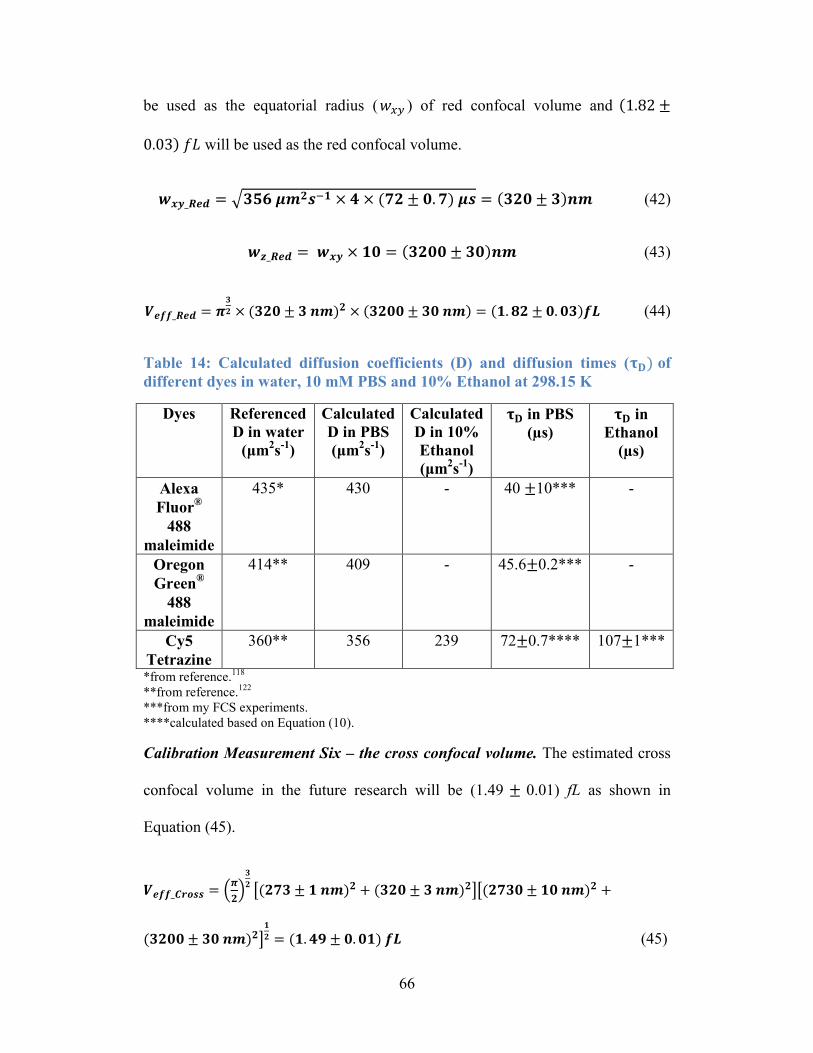
66
be used as the equatorial radius (𝑤𝑥𝑦 ) of red confocal volume and (1.82 ±
0.03) 𝑓𝐿 will be used as the red confocal volume.
𝒘𝒙𝒚_𝑹𝒆𝒅 = √𝟑𝟓𝟔 𝝁𝒎𝟐𝒔−𝟏 × 𝟒 × (𝟕𝟐 ± 𝟎. 𝟕) 𝝁𝒔 = (𝟑𝟐𝟎 ± 𝟑)𝒏𝒎 (42)
𝒘𝒛_𝑹𝒆𝒅 = 𝒘𝒙𝒚 × 𝟏𝟎 = (𝟑𝟐𝟎𝟎 ± 𝟑𝟎)𝒏𝒎 (43)
𝑽𝒆𝒇𝒇_𝑹𝒆𝒅 = 𝝅𝟑
𝟐 × (𝟑𝟐𝟎 ± 𝟑 𝒏𝒎)𝟐 × (𝟑𝟐𝟎𝟎 ± 𝟑𝟎 𝒏𝒎) = (𝟏. 𝟖𝟐 ± 𝟎. 𝟎𝟑)𝒇𝑳 (44)
Table 14: Calculated diffusion coefficients (D) and diffusion times (𝛕𝐃) of
different dyes in water, 10 mM PBS and 10% Ethanol at 298.15 K
Dyes Referenced
D in water
(μm2s
-1)
Calculated
D in PBS
(μm2s
-1)
Calculated
D in 10%
Ethanol
(μm2s
-1)
𝛕𝐃 in PBS
(µs)
𝛕𝐃 in
Ethanol
(µs)
Alexa
Fluor®
488
maleimide
435* 430 - 40 ±10***
-
Oregon
Green®
488
maleimide
414** 409 -
45.6±0.2***
-
Cy5
Tetrazine
360** 356 239 72±0.7**** 107±1***
*from reference.118
**from reference.122
***from my FCS experiments.
****calculated based on Equation (10).
Calibration Measurement Six – the cross confocal volume. The estimated cross
confocal volume in the future research will be (1.49 ± 0.01) fL as shown in
Equation (45).
𝑽𝒆𝒇𝒇_𝑪𝒓𝒐𝒔𝒔 = (𝝅
𝟐)
𝟑
𝟐[(𝟐𝟕𝟑 ± 𝟏 𝒏𝒎)𝟐 + (𝟑𝟐𝟎 ± 𝟑 𝒏𝒎)𝟐][(𝟐𝟕𝟑𝟎 ± 𝟏𝟎 𝒏𝒎)𝟐 +
(𝟑𝟐𝟎𝟎 ± 𝟑𝟎 𝒏𝒎)𝟐]𝟏
𝟐 = (𝟏. 𝟒𝟗 ± 𝟎. 𝟎𝟏) 𝒇𝑳 (45)
67
3.5.2 Hydrodynamic diameters of α-synucleins by FCS
Sample preparations and method. Samples used in this section are monomeric α-
synucleins and the engineered dimers, tetramers and octamers with C-terminal
Cysteine labelled with Oregon Green 488 maleimide or Cy5-tetrazine based on
the sulfhydryl maleimide Reaction Two or Trans-cyclooctenes (TCO) Tetrazine
Reaction. Each sample was measured at the nanomolar concentration and has
more than 50 times of repeat measurements. Each resulting autocorrelation curve
was fitted by the two component autocorrelation function in the defaulted Carl
Zeiss software with suggested fitting parameters. The diffusion time of Oregon
Green 488 maleimide was 45.6 𝜇s, the diffusion time of Cy5 tetrazine was 72 𝜇s,
the fit range started at 1 𝜇𝑠, free triplet state fraction was from 0% to 30%, free
triplet time was from 1 μ𝑠 to 10 μs and 𝑤𝑧
𝑤𝑥𝑦 was equal to 10. All diffusion
coefficients were calculated using Equation (10) with 𝑤𝑥𝑦_𝑔𝑟𝑒𝑒𝑛 = 273 nm and
𝑤𝑥𝑦_𝑟𝑒𝑑 = 320 nm, respectively. All hydrodynamic diameters were calculated
using Equation (11) with T = 298.15 K and viscosity of 10 mM of PBS = 0.00090
Pa·s.
3.5.3 Aggregation tests by FCS
Sample preparations and method. In this section, only monomeric α-synucleins,
the engineered tetramers and Alexa Flour 488 C5 maleimide were ready for the
experiments. Therefore, both proteins were labelled with Alexa Flour 488 C5
maleimide by using the corresponding labelling protocol.
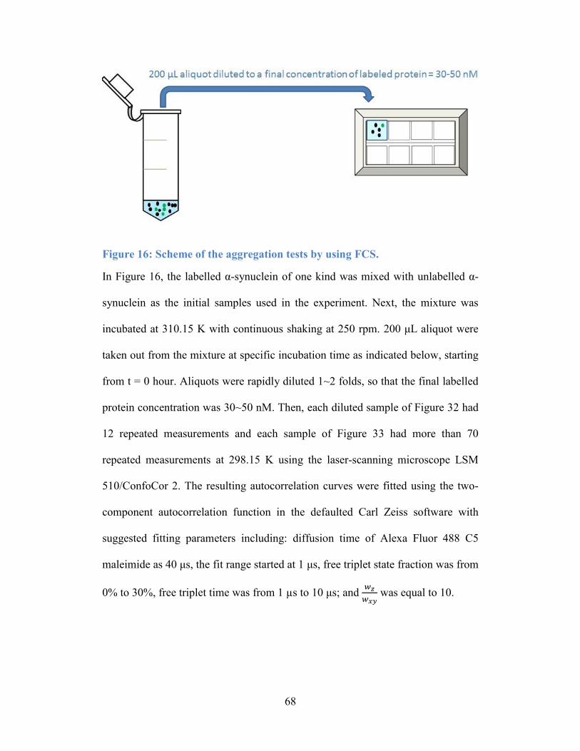
68
Figure 16: Scheme of the aggregation tests by using FCS.
In Figure 16, the labelled α-synuclein of one kind was mixed with unlabelled α-
synuclein as the initial samples used in the experiment. Next, the mixture was
incubated at 310.15 K with continuous shaking at 250 rpm. 200 μL aliquot were
taken out from the mixture at specific incubation time as indicated below, starting
from t = 0 hour. Aliquots were rapidly diluted 1~2 folds, so that the final labelled
protein concentration was 30~50 nM. Then, each diluted sample of Figure 32 had
12 repeated measurements and each sample of Figure 33 had more than 70
repeated measurements at 298.15 K using the laser-scanning microscope LSM
510/ConfoCor 2. The resulting autocorrelation curves were fitted using the two-
component autocorrelation function in the defaulted Carl Zeiss software with
suggested fitting parameters including: diffusion time of Alexa Fluor 488 C5
maleimide as 40 μs, the fit range started at 1 μs, free triplet state fraction was from
0% to 30%, free triplet time was from 1 µs to 10 μs; and 𝑤𝑧
𝑤𝑥𝑦 was equal to 10.
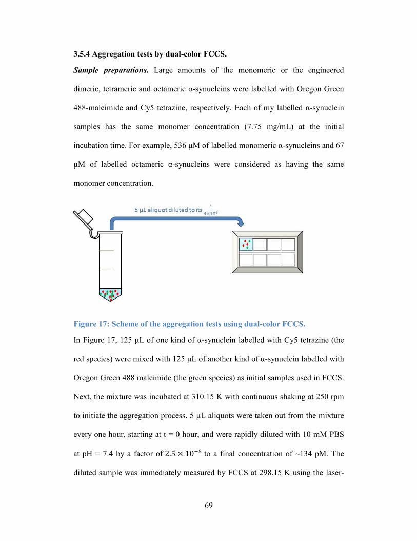
69
3.5.4 Aggregation tests by dual-color FCCS.
Sample preparations. Large amounts of the monomeric or the engineered
dimeric, tetrameric and octameric α-synucleins were labelled with Oregon Green
488-maleimide and Cy5 tetrazine, respectively. Each of my labelled α-synuclein
samples has the same monomer concentration (7.75 mg/mL) at the initial
incubation time. For example, 536 μM of labelled monomeric α-synucleins and 67
μM of labelled octameric α-synucleins were considered as having the same
monomer concentration.
Figure 17: Scheme of the aggregation tests using dual-color FCCS.
In Figure 17, 125 μL of one kind of α-synuclein labelled with Cy5 tetrazine (the
red species) were mixed with 125 μL of another kind of α-synuclein labelled with
Oregon Green 488 maleimide (the green species) as initial samples used in FCCS.
Next, the mixture was incubated at 310.15 K with continuous shaking at 250 rpm
to initiate the aggregation process. 5 μL aliquots were taken out from the mixture
every one hour, starting at t = 0 hour, and were rapidly diluted with 10 mM PBS
at pH = 7.4 by a factor of 2.5 × 10⁻⁵ to a final concentration of ~134 pM. The
diluted sample was immediately measured by FCCS at 298.15 K using the laser-
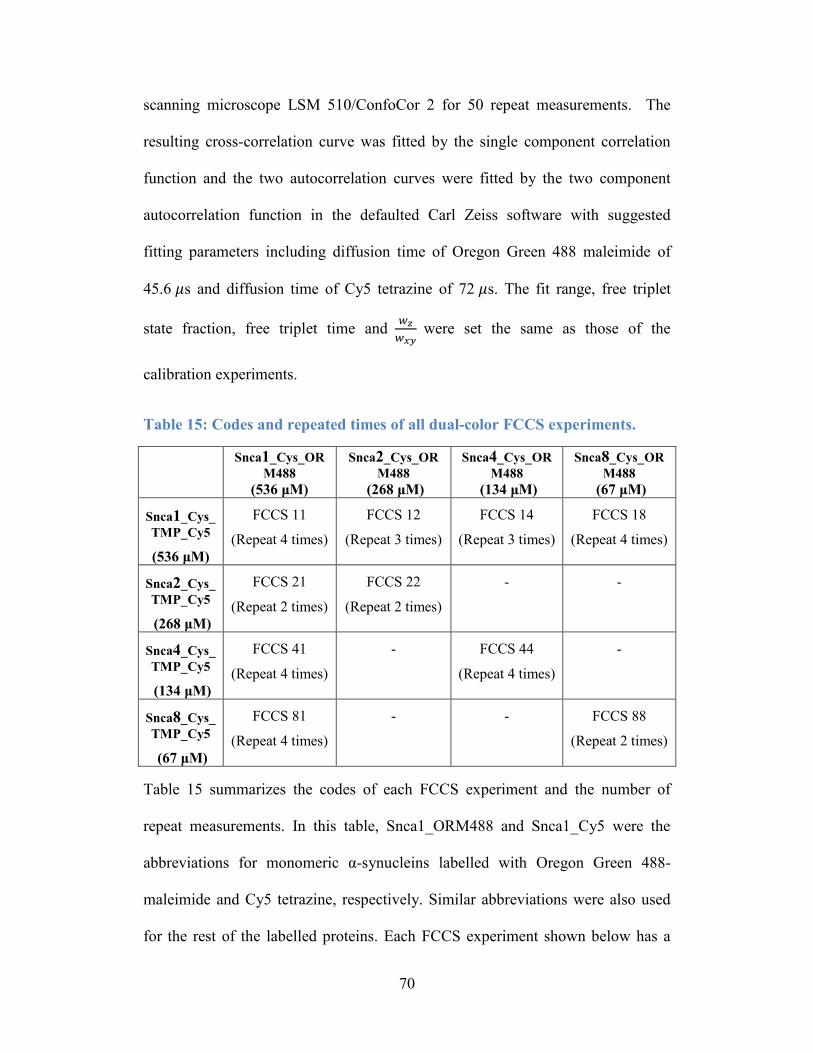
70
scanning microscope LSM 510/ConfoCor 2 for 50 repeat measurements. The
resulting cross-correlation curve was fitted by the single component correlation
function and the two autocorrelation curves were fitted by the two component
autocorrelation function in the defaulted Carl Zeiss software with suggested
fitting parameters including diffusion time of Oregon Green 488 maleimide of
45.6 𝜇s and diffusion time of Cy5 tetrazine of 72 𝜇s. The fit range, free triplet
state fraction, free triplet time and 𝑤𝑧
𝑤𝑥𝑦 were set the same as those of the
calibration experiments.
Table 15: Codes and repeated times of all dual-color FCCS experiments.
Snca1_Cys_OR
M488
(536 μM)
Snca2_Cys_OR
M488
(268 μM)
Snca4_Cys_OR
M488
(134 μM)
Snca8_Cys_OR
M488
(67 μM)
Snca1_Cys_
TMP_Cy5
(536 μM)
FCCS 11
(Repeat 4 times)
FCCS 12
(Repeat 3 times)
FCCS 14
(Repeat 3 times)
FCCS 18
(Repeat 4 times)
Snca2_Cys_
TMP_Cy5
(268 μM)
FCCS 21
(Repeat 2 times)
FCCS 22
(Repeat 2 times)
- -
Snca4_Cys_
TMP_Cy5
(134 μM)
FCCS 41
(Repeat 4 times)
- FCCS 44
(Repeat 4 times)
-
Snca8_Cys_
TMP_Cy5
(67 μM)
FCCS 81
(Repeat 4 times)
- - FCCS 88
(Repeat 2 times)
Table 15 summarizes the codes of each FCCS experiment and the number of
repeat measurements. In this table, Snca1_ORM488 and Snca1_Cy5 were the
abbreviations for monomeric α-synucleins labelled with Oregon Green 488-
maleimide and Cy5 tetrazine, respectively. Similar abbreviations were also used
for the rest of the labelled proteins. Each FCCS experiment shown below has a
71
name in the format of “FCCS xx”, the first digits of which indicates the type of α-
synuclein labelled with Cy5 tetrazine. For example, the FCCS experiment was
called “FCCS 41”, when tetrameric α-synuclein with Cy5 tetrazine and
monomeric α-synucleins with Oregon Green 488-maleimide were the initial red
and green species.
Finally, in order to understand whether continuous shaking could affect the
aggregation process, 125 μL of octameric α-synuclein (67 μM) labelled with Cy5
tetrazine were mixed with 125 μL of octameric α-synuclein (67 μM) labelled with
Oregon Green 488 maleimide (the green species), and then it was incubated of
310.15 K without shaking as a control group. Each controlled experiment of the
same sample was measured for 50 times and each control group with newly made
sample was repeated one more time.
Data analysis. Equations (46) and (47) were obtained after rearrange of Equation
(17).
𝑵𝒓𝒈
𝑵𝒓=
𝑮𝒓𝒈(𝟎)
𝑮𝒈(𝟎) (46)
𝑵𝒓𝒈
𝑵𝒈=
𝑮𝒓𝒈(𝟎)
𝑮𝒓(𝟎) (47)
where 𝑁𝑟𝑔 is the absolute number of fluorescent aggregates observed within the
cross confocal volume, 𝑁𝑟 is the absolute number of red fluorescent species
observed within the red confocal volume and 𝑁𝑔 is the absolute number of green
fluorescent species observed within the green confocal volume. The physical
72
meaning of 𝑁𝑟𝑔
𝑁𝑟 refers as the fraction of red fluorescent species which were used to
form conjugates. It is advantageous to present FCCS data in the format 𝑁𝑟𝑔
𝑁𝑟
instead of using the absolute number. Dilution of a very small amount of aliquot
(5 μL) caused large errors between the absolute numbers of fluorescent species
observed under confocal volume (𝑁) at different incubation timeS for each FCCS
experiment. Presenting FCCS data as 𝑁𝑟𝑔
𝑁𝑟 or
𝑁𝑟𝑔
𝑁𝑔 solves the problem. Considering
the slight difference between the red, green and cross confocal volumes, ⟨𝑛𝑟⟩, ⟨𝑛𝑔⟩
and ⟨𝑛𝑟𝑔⟩ were used to correct for the different confocal volume as shown in
Equations (48) and (49).
⟨𝒏𝒓𝒈⟩
⟨𝒏𝒓⟩=
𝑮𝒓𝒈(𝟎)
𝑮𝒈(𝟎)×
𝑽𝒆𝒇𝒇_𝑹𝒆𝒅
𝑽𝒆𝒇𝒇_𝑪𝒓𝒐𝒔𝒔=
𝑮𝒓𝒈(𝟎)
𝑮𝒈(𝟎)×
𝟏.𝟖𝟐
𝟏.𝟒𝟗× 𝟏𝟎𝟎% (48)
⟨𝒏𝒓𝒈⟩
⟨𝒏𝒈⟩=
𝑮𝒓𝒈(𝟎)
𝑮𝒓(𝟎)×
𝑽𝒆𝒇𝒇_𝑮𝒓𝒆𝒆𝒏
𝑽𝒆𝒇𝒇_𝑪𝒓𝒐𝒔𝒔=
𝑮𝒓𝒈(𝟎)
𝑮𝒓(𝟎)×
𝟏.𝟏𝟑𝟓
𝟏.𝟒𝟗× 𝟏𝟎𝟎% (49)
The final FCCS aggregation data was represented as a plot of ⟨𝑛𝑟𝑔⟩
⟨𝑛𝑟⟩ or
⟨𝑛𝑟𝑔⟩
⟨𝑛𝑔⟩ as a
function of the incubation time. Then an exponential growth function, Equation
(50), was used to fit the plot.
𝒚 = 𝒚𝟎 + 𝑨 × (𝟏 − 𝒆(−𝒙∙𝒌)) (50)
From the fitting curves, two important values were obtained: (i) the amplitude of
the fitting curve, 𝐴 , which gives the difference between the start-point and
endpoint of each aggregation test; and (ii) the parameter, 𝑘 , which is the

73
reciprocal of the growth time. The growth time is defined as the time to reach 1
𝑒 of
the final value.
74
Chapter 4: Results and Discussions
The objective of this research is to establish a generic approach to study the
aggregation between engineered α-synuclein oligomers and monomers using dual-
color FCCS. To do this, several experiments are conducted. These experiments
include: (i) properly labelling of the protein of interest; (ii) efficiently purifing the
labelled protein; (iii) ensuring the quantum yields of fluorescent dyes keep
constant once they are mixed with or bind to the protein of interest; (iv) measuring
the initial hydrodynamic size of the protein of interest before aggregation by DLS;
(v) validating the initial hydrodynamic size of the protein by FCS; and (vi)
monitoring the aggregation process between the engineer α-synuclein oligomers
and monomer by both FCS and dual-color FCCS. All experimental results are
summarized in this Chapter.
4.1 Purification and labelling efficiency
4.1.1 Distinguishing non-specific binding from covalent labelling
Results. To ensure that unconjugated dye and protein were baseline-separated,
each FPLC purification experiment was conducted with three control samples: (i)
the dye; (ii) the α-synuclein before labelling; and (iii) the mixture of unlabelled α-
synuclein and the dye.
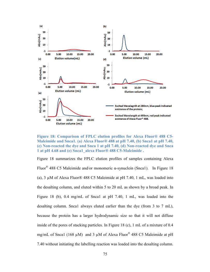
75
Figure 18: Comparison of FPLC elution profiles for Alexa Fluor® 488 C5-
Maleimide and Snca1. (a) Alexa Fluor® 488 at pH 7.40, (b) Snca1 at pH 7.40,
(c) Non-reacted the dye and Snca 1 at pH 7.40, (d) Non-reacted dye and Snca
1 at pH 4.68 and (e) Snca1_alexa Fluor® 488 C5-Maleimide .
Figure 18 summarizes the FPLC elution profiles of samples containing Alexa
Fluor®
488 C5 Maleimide and/or monomeric α-synuclein (Snca1). In Figure 18
(a), 3 µM of Alexa Fluor® 488 C5 Maleimide at pH 7.40, 1 mL, was loaded into
the desalting column, and eluted within 5 to 20 mL as shown by a broad peak. In
Figure 18 (b), 0.4 mg/mL of Snca1 at pH 7.40, 1 mL, was loaded into the
desalting column. Snca1 always eluted earlier than the dye (from 3 to 7 mL),
because the protein has a larger hydrodynamic size so that it will not diffuse
inside of the pores of stacking particles. In Figure 18 (c), 1 mL of a mixture of 0.4
mg/mL of Snca1 (168 µM) and 3 µM of Alexa Fluor® 488 C5 Maleimide at pH
7.40 without initiating the labelling reaction was loaded into the desalting column.
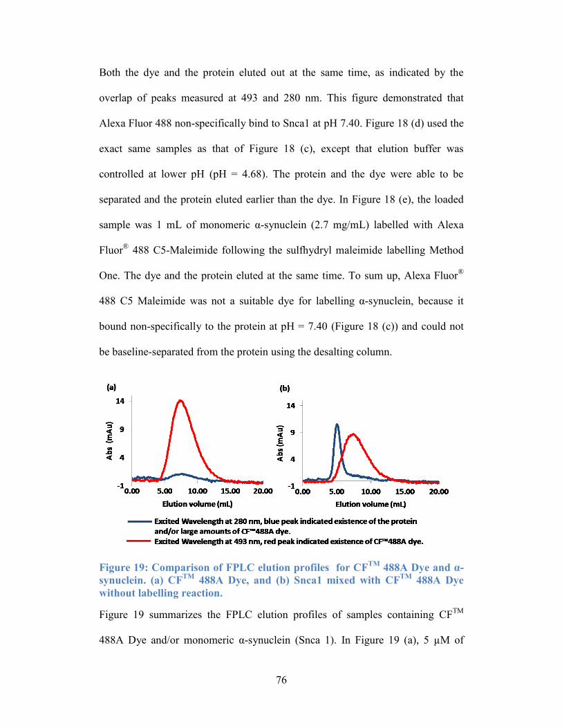
76
Both the dye and the protein eluted out at the same time, as indicated by the
overlap of peaks measured at 493 and 280 nm. This figure demonstrated that
Alexa Fluor 488 non-specifically bind to Snca1 at pH 7.40. Figure 18 (d) used the
exact same samples as that of Figure 18 (c), except that elution buffer was
controlled at lower pH (pH = 4.68). The protein and the dye were able to be
separated and the protein eluted earlier than the dye. In Figure 18 (e), the loaded
sample was 1 mL of monomeric α-synuclein (2.7 mg/mL) labelled with Alexa
Fluor®
488 C5-Maleimide following the sulfhydryl maleimide labelling Method
One. The dye and the protein eluted at the same time. To sum up, Alexa Fluor®
488 C5 Maleimide was not a suitable dye for labelling α-synuclein, because it
bound non-specifically to the protein at pH = 7.40 (Figure 18 (c)) and could not
be baseline-separated from the protein using the desalting column.
Figure 19: Comparison of FPLC elution profiles for CFTM
488A Dye and α-
synuclein. (a) CFTM
488A Dye, and (b) Snca1 mixed with CFTM
488A Dye
without labelling reaction.
Figure 19 summarizes the FPLC elution profiles of samples containing CFTM
488A Dye and/or monomeric α-synuclein (Snca 1). In Figure 19 (a), 5 µM of
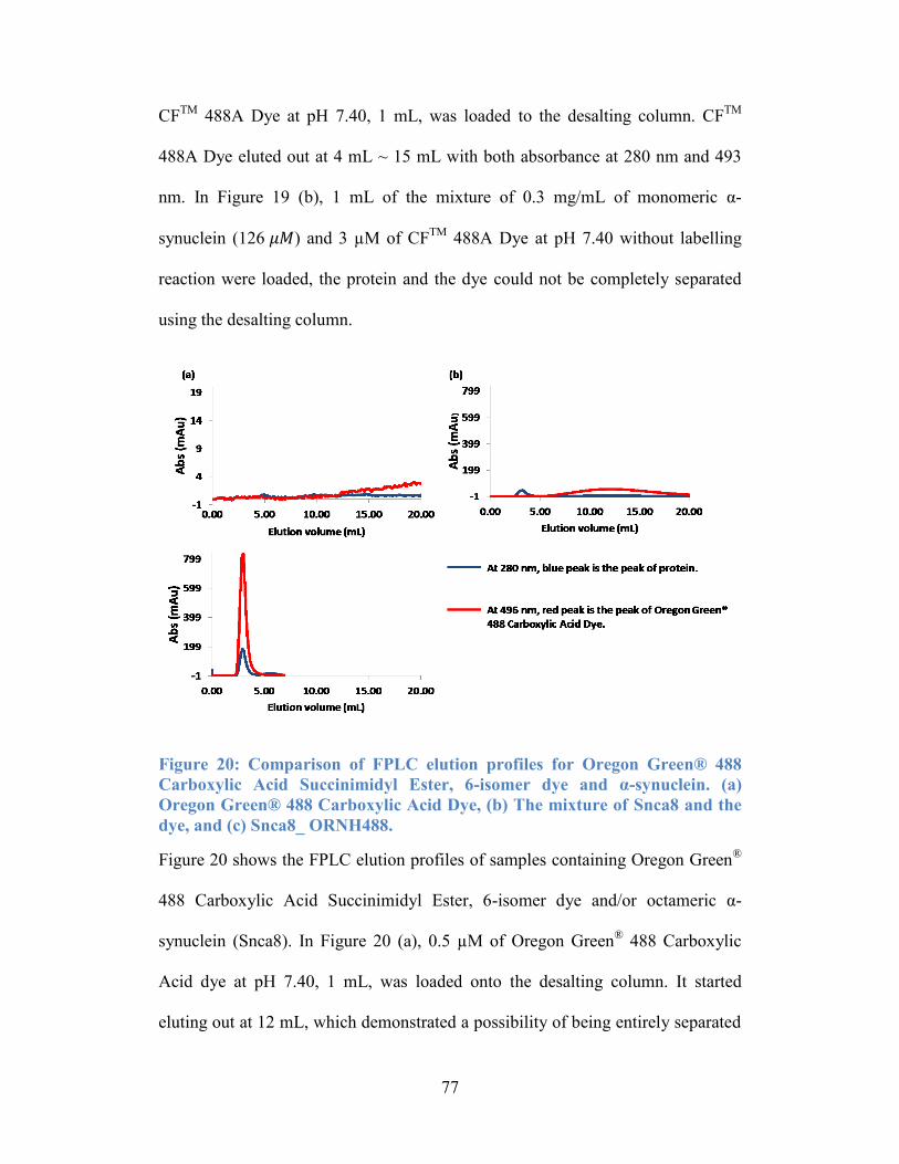
77
CFTM
488A Dye at pH 7.40, 1 mL, was loaded to the desalting column. CFTM
488A Dye eluted out at 4 mL ~ 15 mL with both absorbance at 280 nm and 493
nm. In Figure 19 (b), 1 mL of the mixture of 0.3 mg/mL of monomeric α-
synuclein (126 𝜇𝑀) and 3 µM of CFTM
488A Dye at pH 7.40 without labelling
reaction were loaded, the protein and the dye could not be completely separated
using the desalting column.
Figure 20: Comparison of FPLC elution profiles for Oregon Green® 488
Carboxylic Acid Succinimidyl Ester, 6-isomer dye and α-synuclein. (a)
Oregon Green® 488 Carboxylic Acid Dye, (b) The mixture of Snca8 and the
dye, and (c) Snca8_ ORNH488.
Figure 20 shows the FPLC elution profiles of samples containing Oregon Green®
488 Carboxylic Acid Succinimidyl Ester, 6-isomer dye and/or octameric α-
synuclein (Snca8). In Figure 20 (a), 0.5 µM of Oregon Green®
488 Carboxylic
Acid dye at pH 7.40, 1 mL, was loaded onto the desalting column. It started
eluting out at 12 mL, which demonstrated a possibility of being entirely separated
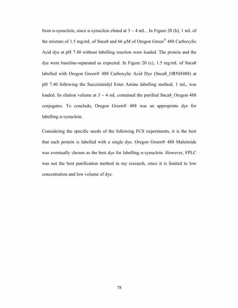
78
from α-synuclein, since α-synuclein eluted at 3 ~ 4 mL . In Figure 20 (b), 1 mL of
the mixture of 1.5 mg/mL of Snca8 and 66 µM of Oregon Green® 488 Carboxylic
Acid dye at pH 7.40 without labelling reaction were loaded. The protein and the
dye were baseline-separated as expected. In Figure 20 (c), 1.5 mg/mL of Snca8
labelled with Oregon Green® 488 Carboxylic Acid Dye (Snca8_ORNH488) at
pH 7.40 following the Succinimidyl Ester Amine labelling method, 1 mL, was
loaded. Its elution volume at 3 ~ 4 mL contained the purified Snca8_Oregon 488
conjugates. To conclude, Oregon Green® 488 was an appropriate dye for
labelling α-synuclein.
Considering the specific needs of the following FCS experiments, it is the best
that each protein is labelled with a single dye. Oregon Green® 488 Maleimide
was eventually chosen as the best dye for labelling α-synuclein. However, FPLC
was not the best purification method in my research, since it is limited to low
concentration and low volume of dye.
79
Figure 21: Comparison of FPLC elution profiles for Oregon Green® 488
Maleimide and α-synuclein. (a) Snca4_ORM488 using sulfhydryl maleimide
labelling Method One. (b) Snca4_ORM488 using sulfhydryl maleimide
labelling Method Two.
Figure 21 demonstrates two FPLC elution profiles of tetrameric α-synuclein
labelled with Oregon Green® 488 Maleimide (Snca4_ORM488). In Figure 21 (a),
1 mL of 2 mg/mL Snca4 labelled with Oregon Green® 488 Maleimide Dye at pH
7.40 followed by the sulfhydryl maleimide labelling Method One. Unfortunately,
the labelled protein and the free dye could not be completely separated, since peak
of the protein and dye slightly overlapped which is due to the large amounts of
dye. In Figure 21 (b), the same amounts of protein were labelled with Oregon
Green® 488 Maleimide Dye at pH 7.40 followed by the sulfhydryl maleimide
labelling Method Two, the labelled protein and the free dye could be completely
separated, because less dyes were used for labelling.
Discussion. The results reported above confirm that Alexa Fluor® 488 C5
Maleimide and CFTM
488A Dye bind non-specifically with α-synuclein at pH 7.40
and these cannot be separated from the protein using the desalting column. The
80
non-specific binding between the dye and α-synuclein is probably due to
electrostatic interactions between the charged dyes and the charged α-synuclein.
This hypothesis is supported by the result that Alexa Fluor® 488 C5 Maleimide
and α-synuclein can be largely separated at low pH, when the charge distributions
of α-synuclein are completely changed (anionic Alexa Fluor 488 appears fully
ionized within pH 3~10).123
Therefore, Oregon Green® 488 Maleimide, as an
uncharged dye, is the best dye for labelling α-synuclein.
The above results also show that FPLC is not the best protein purification method
for this protein system. It is able to measure absorbance of each small eluted
fraction volume automatically, but it is limited in purifying small quantities of
labelled α-synuclein at each sample run. Because higher concentrations of
fluorescent dye are required for labelling large quantities of α-synuclein for the
future aggregation tests, other purification methods were explored.
4.1.2 High labelling efficiency demonstrated by centrifugal purification
Selected experimental results. Based on the FPLC results, Alexa Fluor® 488 were
bound non-specifically with α-synuclein under “physiological” conditions (10
mM PBS at pH = 7.4). Therefore, only Oregon Green 488 maleimide and Cy5
tetrazine were used to label the engineered α-synuclein monomer and oligomers in
this section and these labelled proteins were used in subsequent aggregation tests.
Some selected results presented below demonstrate how well both dyes
conjugated with the protein and that excess dyes could be effectively removed.
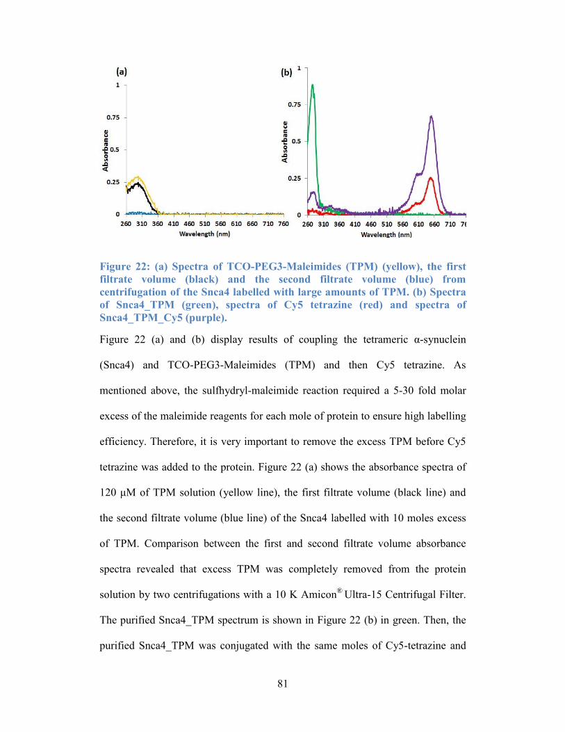
81
Figure 22: (a) Spectra of TCO-PEG3-Maleimides (TPM) (yellow), the first
filtrate volume (black) and the second filtrate volume (blue) from
centrifugation of the Snca4 labelled with large amounts of TPM. (b) Spectra
of Snca4_TPM (green), spectra of Cy5 tetrazine (red) and spectra of
Snca4_TPM_Cy5 (purple).
Figure 22 (a) and (b) display results of coupling the tetrameric α-synuclein
(Snca4) and TCO-PEG3-Maleimides (TPM) and then Cy5 tetrazine. As
mentioned above, the sulfhydryl-maleimide reaction required a 5-30 fold molar
excess of the maleimide reagents for each mole of protein to ensure high labelling
efficiency. Therefore, it is very important to remove the excess TPM before Cy5
tetrazine was added to the protein. Figure 22 (a) shows the absorbance spectra of
120 μM of TPM solution (yellow line), the first filtrate volume (black line) and
the second filtrate volume (blue line) of the Snca4 labelled with 10 moles excess
of TPM. Comparison between the first and second filtrate volume absorbance
spectra revealed that excess TPM was completely removed from the protein
solution by two centrifugations with a 10 K Amicon®
Ultra-15 Centrifugal Filter.
The purified Snca4_TPM spectrum is shown in Figure 22 (b) in green. Then, the
purified Snca4_TPM was conjugated with the same moles of Cy5-tetrazine and
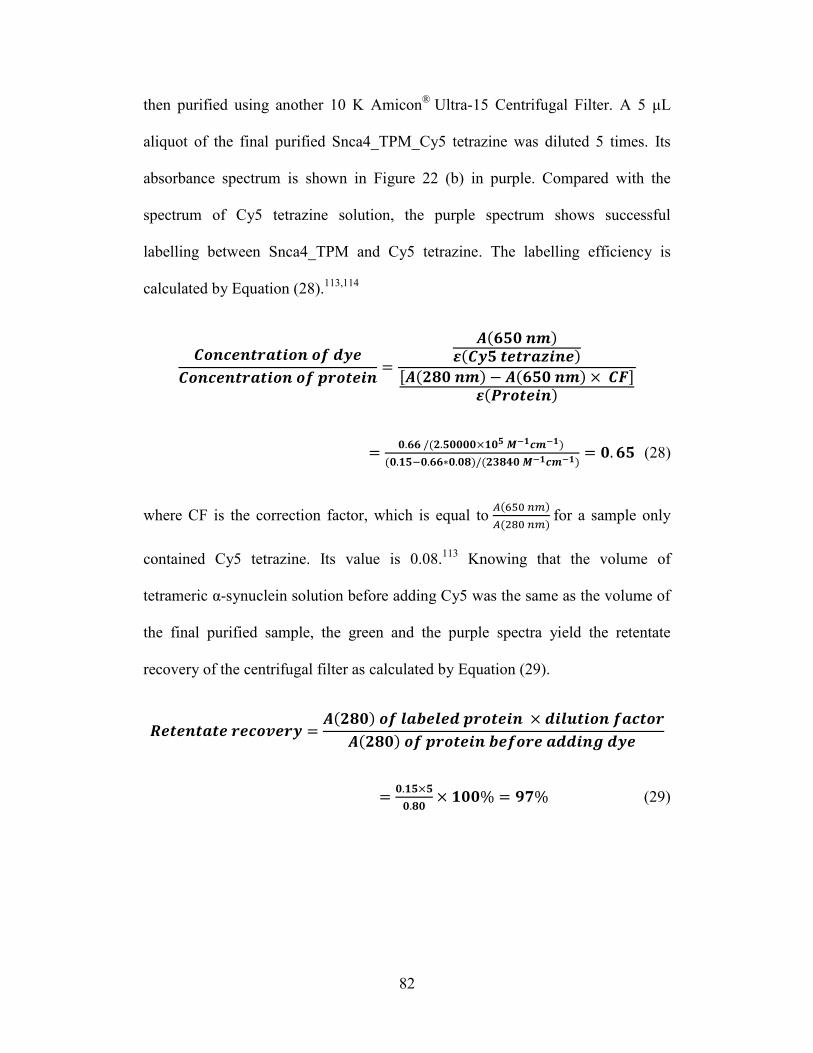
82
then purified using another 10 K Amicon®
Ultra-15 Centrifugal Filter. A 5 μL
aliquot of the final purified Snca4_TPM_Cy5 tetrazine was diluted 5 times. Its
absorbance spectrum is shown in Figure 22 (b) in purple. Compared with the
spectrum of Cy5 tetrazine solution, the purple spectrum shows successful
labelling between Snca4_TPM and Cy5 tetrazine. The labelling efficiency is
calculated by Equation (28).113,114
𝑪𝒐𝒏𝒄𝒆𝒏𝒕𝒓𝒂𝒕𝒊𝒐𝒏 𝒐𝒇 𝒅𝒚𝒆
𝑪𝒐𝒏𝒄𝒆𝒏𝒕𝒓𝒂𝒕𝒊𝒐𝒏 𝒐𝒇 𝒑𝒓𝒐𝒕𝒆𝒊𝒏=
𝑨(𝟔𝟓𝟎 𝒏𝒎)𝜺(𝑪𝒚𝟓 𝒕𝒆𝒕𝒓𝒂𝒛𝒊𝒏𝒆)
[𝑨(𝟐𝟖𝟎 𝒏𝒎) − 𝑨(𝟔𝟓𝟎 𝒏𝒎) × 𝑪𝑭]𝜺(𝑷𝒓𝒐𝒕𝒆𝒊𝒏)
=𝟎.𝟔𝟔 /(𝟐.𝟓𝟎𝟎𝟎𝟎×𝟏𝟎𝟓 𝑴−𝟏𝒄𝒎−𝟏)
(𝟎.𝟏𝟓−𝟎.𝟔𝟔∗𝟎.𝟎𝟖)/(𝟐𝟑𝟖𝟒𝟎 𝑴−𝟏𝒄𝒎−𝟏)= 𝟎. 𝟔𝟓 (28)
where CF is the correction factor, which is equal to 𝐴(650 𝑛𝑚)
𝐴(280 𝑛𝑚) for a sample only
contained Cy5 tetrazine. Its value is 0.08.113
Knowing that the volume of
tetrameric α-synuclein solution before adding Cy5 was the same as the volume of
the final purified sample, the green and the purple spectra yield the retentate
recovery of the centrifugal filter as calculated by Equation (29).
𝑹𝒆𝒕𝒆𝒏𝒕𝒂𝒕𝒆 𝒓𝒆𝒄𝒐𝒗𝒆𝒓𝒚 =𝑨(𝟐𝟖𝟎) 𝒐𝒇 𝒍𝒂𝒃𝒆𝒍𝒆𝒅 𝒑𝒓𝒐𝒕𝒆𝒊𝒏 × 𝒅𝒊𝒍𝒖𝒕𝒊𝒐𝒏 𝒇𝒂𝒄𝒕𝒐𝒓
𝑨(𝟐𝟖𝟎) 𝒐𝒇 𝒑𝒓𝒐𝒕𝒆𝒊𝒏 𝒃𝒆𝒇𝒐𝒓𝒆 𝒂𝒅𝒅𝒊𝒏𝒈 𝒅𝒚𝒆
=𝟎.𝟏𝟓×𝟓
𝟎.𝟖𝟎× 𝟏𝟎𝟎% = 𝟗𝟕% (29)
83
Figure 23: Spectra of Oregon Green 488 maleimide (green), Snca4 before
labelling (yellow) and 5 µL of Snca4_ORM488 diluted by 20 times (purple).
Figure 23 demonstrates a removal of excess Oregon Green 488 maleimide from
tetrameric α-synuclein (Snca 4) solution by centrifugation. The figure shows the
spectra of samples that contained only Oregon Green 488 maleimde (green line),
only Snca 4 (yellow line) and of a 5 µL Snca 4_ORM488 aliquot diluted by 20
times (purple line). Comparing the green and the purple spectra at 493 𝑛𝑚
and 280 𝑛𝑚, a successful conjugation between tetrameric α-synuclein and Oregon
Green 488 maleimde is demonstrated. Its labelling efficiency is calculated by
Equation (30).
84
𝑪𝒐𝒏𝒄𝒆𝒏𝒕𝒓𝒂𝒕𝒊𝒐𝒏 𝒐𝒇 𝒅𝒚𝒆
𝑪𝒐𝒏𝒄𝒆𝒏𝒕𝒓𝒂𝒕𝒊𝒐𝒏 𝒐𝒇 𝒑𝒓𝒐𝒕𝒆𝒊𝒏=
𝑨(𝟒𝟗𝟐 𝒏𝒎)𝜺(𝑶𝒓𝒆𝒈𝒐𝒏 𝟒𝟖𝟖)
[𝑨(𝟐𝟖𝟎 𝒏𝒎) − 𝑨(𝟒𝟗𝟐 𝒏𝒎) × 𝑪𝑭]𝜺(𝑷𝒓𝒐𝒕𝒆𝒊𝒏)
=𝟎.𝟐𝟑 /(𝟖.𝟕𝟎𝟎𝟎×𝟏𝟎𝟒 𝑴−𝟏𝒄𝒎−𝟏)
(𝟎.𝟏𝟎−𝟎.𝟐𝟑∗𝟎.𝟏𝟐)/ (𝟐𝟑𝟖𝟒𝟎 𝑴−𝟏𝒄𝒎−𝟏)= 𝟎. 𝟗𝟕 (30)
Discussion. To sum up, the Amicon®
Ultra Centrifugal Filters with centrifugation
is a faster and cleaner method to remove excess dyes and TPM from the α-
synuclein solution, especially when large quantities of protein are labelled. It also
shows a very high protein recovery after purification. More importantly, in
combination with an Agilent Cary 60 UV/Vis spectrophotometer, only very small
aliquots (5 ~ 100 μL) of final samples are needed to obtain protein concentration
and labelling efficiency.
4.1.3 HPLC-MS confirms covalent labelling at high efficiency
Experimental data. Figure 24 is a MS spectrum consisted of both labelled and
unlabelled monomeric α-synuclein. The multiple small peaks of one large peak
indicate differing numbers of methionine of the protein that were oxidized during
the electrospray ionization. Therefore, there always was a mass difference around
16 Da between the nearby peaks arising from an addition of oxygen atom.
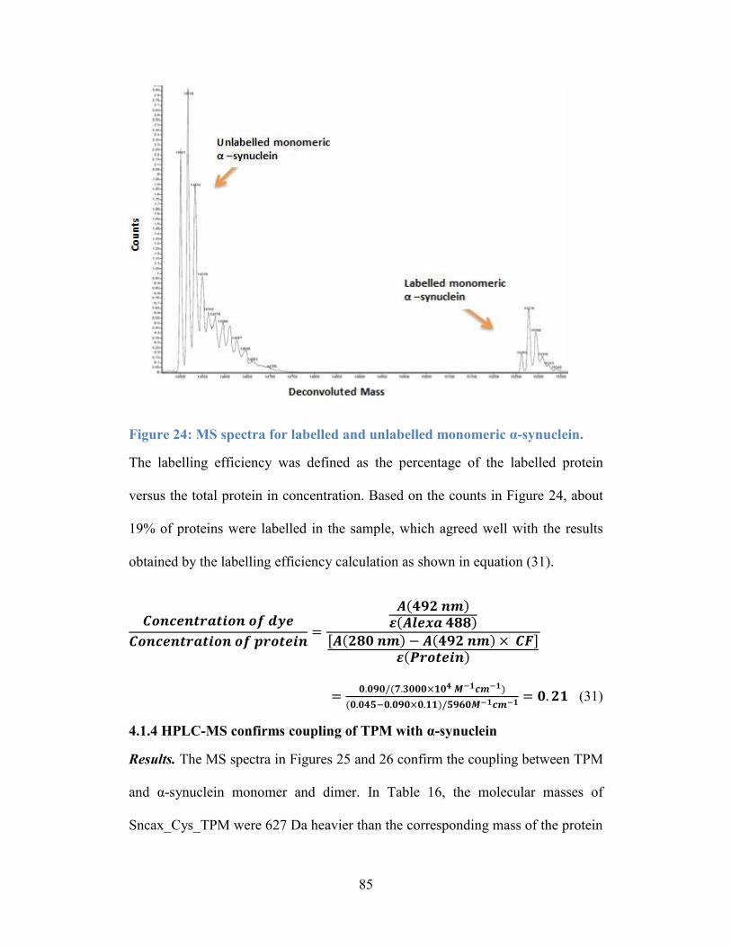
85
Figure 24: MS spectra for labelled and unlabelled monomeric α-synuclein.
The labelling efficiency was defined as the percentage of the labelled protein
versus the total protein in concentration. Based on the counts in Figure 24, about
19% of proteins were labelled in the sample, which agreed well with the results
obtained by the labelling efficiency calculation as shown in equation (31).
𝑪𝒐𝒏𝒄𝒆𝒏𝒕𝒓𝒂𝒕𝒊𝒐𝒏 𝒐𝒇 𝒅𝒚𝒆
𝑪𝒐𝒏𝒄𝒆𝒏𝒕𝒓𝒂𝒕𝒊𝒐𝒏 𝒐𝒇 𝒑𝒓𝒐𝒕𝒆𝒊𝒏=
𝑨(𝟒𝟗𝟐 𝒏𝒎)𝜺(𝑨𝒍𝒆𝒙𝒂 𝟒𝟖𝟖)
[𝑨(𝟐𝟖𝟎 𝒏𝒎) − 𝑨(𝟒𝟗𝟐 𝒏𝒎) × 𝑪𝑭]𝜺(𝑷𝒓𝒐𝒕𝒆𝒊𝒏)
=𝟎.𝟎𝟗𝟎/(𝟕.𝟑𝟎𝟎𝟎×𝟏𝟎𝟒 𝑴−𝟏𝒄𝒎−𝟏)
(𝟎.𝟎𝟒𝟓−𝟎.𝟎𝟗𝟎×𝟎.𝟏𝟏)/𝟓𝟗𝟔𝟎𝑴−𝟏𝒄𝒎−𝟏 = 𝟎. 𝟐𝟏 (31)
4.1.4 HPLC-MS confirms coupling of TPM with α-synuclein
Results. The MS spectra in Figures 25 and 26 confirm the coupling between TPM
and α-synuclein monomer and dimer. In Table 16, the molecular masses of
Sncax_Cys_TPM were 627 Da heavier than the corresponding mass of the protein
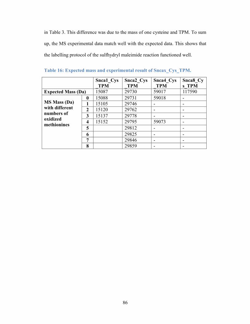
86
in Table 3. This difference was due to the mass of one cysteine and TPM. To sum
up, the MS experimental data match well with the expected data. This shows that
the labelling protocol of the sulfhydryl maleimide reaction functioned well.
Table 16: Expected mass and experimental result of Sncax_Cys_TPM.
Snca1_Cys
_TPM
Snca2_Cys
_TPM
Snca4_Cys
_TPM
Snca8_Cy
s_TPM
Expected Mass (Da) 15087 29730 59017 117590
MS Mass (Da)
with different
numbers of
oxidized
methionines
0 15088 29731 59018 -
1 15105 29746 - -
2 15120 29762 - -
3 15137 29778 - -
4 15152 29795 59073 -
5 29812 - -
6 29825 - -
7 29846 - -
8 29859 - -
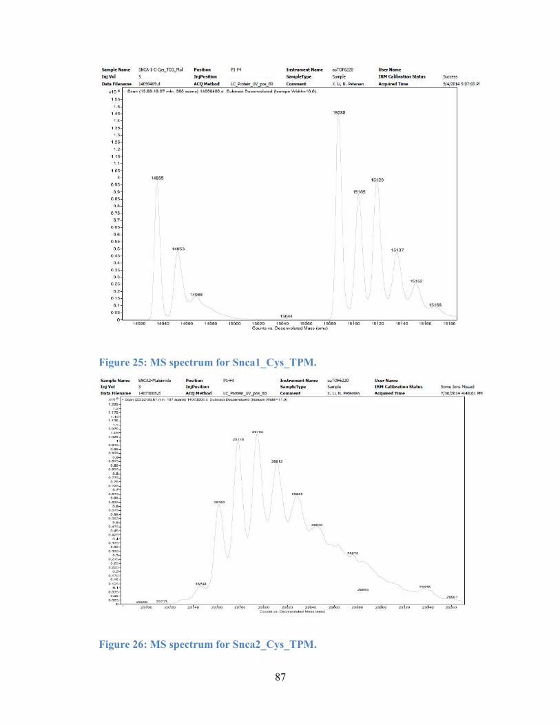
87
Figure 25: MS spectrum for Snca1_Cys_TPM.
Figure 26: MS spectrum for Snca2_Cys_TPM.
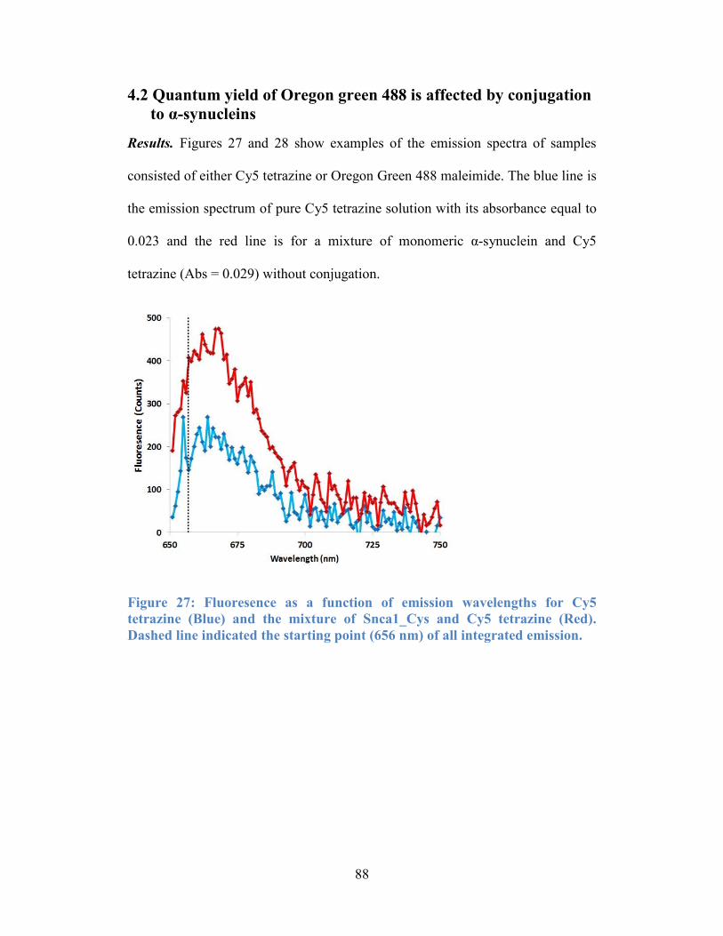
88
4.2 Quantum yield of Oregon green 488 is affected by conjugation
to α-synucleins
Results. Figures 27 and 28 show examples of the emission spectra of samples
consisted of either Cy5 tetrazine or Oregon Green 488 maleimide. The blue line is
the emission spectrum of pure Cy5 tetrazine solution with its absorbance equal to
0.023 and the red line is for a mixture of monomeric α-synuclein and Cy5
tetrazine (Abs = 0.029) without conjugation.
Figure 27: Fluoresence as a function of emission wavelengths for Cy5
tetrazine (Blue) and the mixture of Snca1_Cys and Cy5 tetrazine (Red).
Dashed line indicated the starting point (656 nm) of all integrated emission.
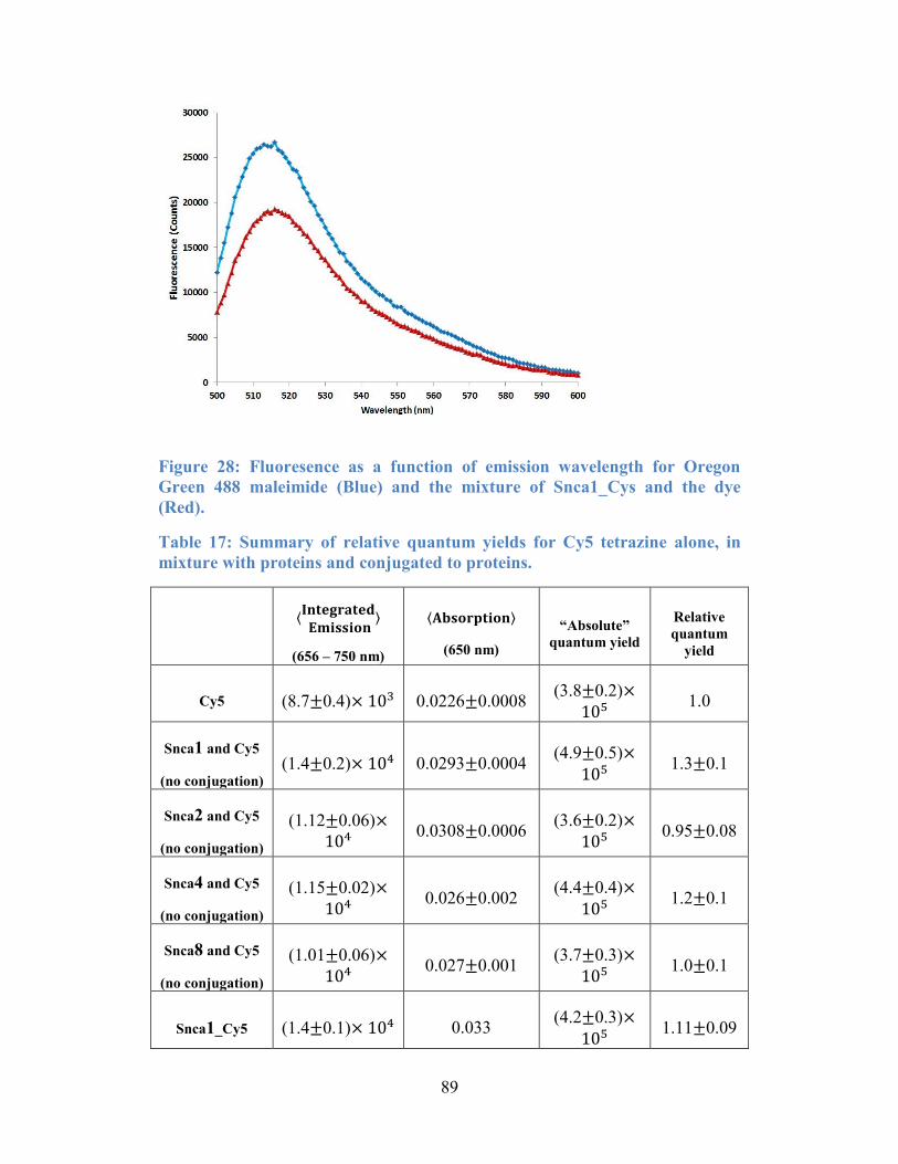
89
Figure 28: Fluoresence as a function of emission wavelength for Oregon
Green 488 maleimide (Blue) and the mixture of Snca1_Cys and the dye
(Red).
Table 17: Summary of relative quantum yields for Cy5 tetrazine alone, in
mixture with proteins and conjugated to proteins.
⟨𝐈𝐧𝐭𝐞𝐠𝐫𝐚𝐭𝐞𝐝 𝐄𝐦𝐢𝐬𝐬𝐢𝐨𝐧
⟩
(656 – 750 nm)
⟨𝐀𝐛𝐬𝐨𝐫𝐩𝐭𝐢𝐨𝐧⟩
(650 nm)
“Absolute”
quantum yield
Relative
quantum
yield
Cy5 (8.7±0.4)× 103 0.0226±0.0008 (3.8±0.2)×
105 1.0
Snca1 and Cy5
(no conjugation)
(1.4±0.2)× 104 0.0293±0.0004 (4.9±0.5)×
105 1.3±0.1
Snca2 and Cy5
(no conjugation)
(1.12±0.06)×104
0.0308±0.0006 (3.6±0.2)×
105 0.95±0.08
Snca4 and Cy5
(no conjugation)
(1.15±0.02)×104
0.026±0.002 (4.4±0.4)×
105 1.2±0.1
Snca8 and Cy5
(no conjugation)
(1.01±0.06)×104
0.027±0.001 (3.7±0.3)×
105 1.0±0.1
Snca1_Cy5 (1.4±0.1)× 104 0.033 (4.2±0.3)×
105 1.11±0.09
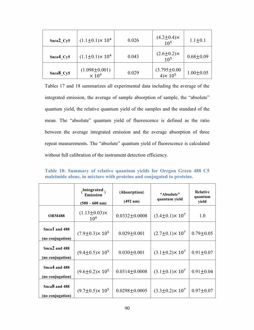
90
Snca2_Cy5 (1.1±0.1)× 104 0.026 (4.2±0.4)×
105 1.1±0.1
Snca4_Cy5 (1.1±0.1)× 104 0.043 (2.6±0.2)×
105 0.68±0.09
Snca8_Cy5 (1.098±0.001)
× 104 0.029
(3.795±0.00
4)× 105 1.00±0.05
Tables 17 and 18 summarizes all experimental data including the average of the
integrated emission, the average of sample absorption of sample, the “absolute”
quantum yield, the relative quantum yield of the samples and the standard of the
mean. The “absolute” quantum yield of fluorescence is defined as the ratio
between the average integrated emission and the average absorption of three
repeat measurements. The “absolute” quantum yield of fluorescence is calculated
without full calibration of the instrument detection efficiency.
Table 18: Summary of relative quantum yields for Oregon Green 488 C5
maleimide alone, in mixture with proteins and conjugated to proteins.
⟨𝐈𝐧𝐭𝐞𝐠𝐫𝐚𝐭𝐞𝐝
𝐄𝐦𝐢𝐬𝐬𝐢𝐨𝐧⟩
(500 – 600 nm)
⟨𝐀𝐛𝐬𝐨𝐫𝐩𝐭𝐢𝐨𝐧⟩
(492 nm)
“Absolute”
quantum yield
Relative
quantum
yield
ORM488 (1.13±0.03)×
106 0.0332±0.0008 (3.4±0.1)× 107 1.0
Snca1 and 488
(no conjugation)
(7.9±0.3)× 105 0.029±0.001 (2.7±0.1)× 107 0.79±0.05
Snca2 and 488
(no conjugation)
(9.4±0.5)× 105 0.030±0.001 (3.1±0.2)× 107 0.91±0.07
Snca4 and 488
(no conjugation)
(9.6±0.2)× 105 0.0314±0.0008 (3.1±0.1)× 107 0.91±0.04
Snca8 and 488
(no conjugation)
(9.7±0.5)× 105 0.0298±0.0005 (3.3±0.2)× 107 0.97±0.07
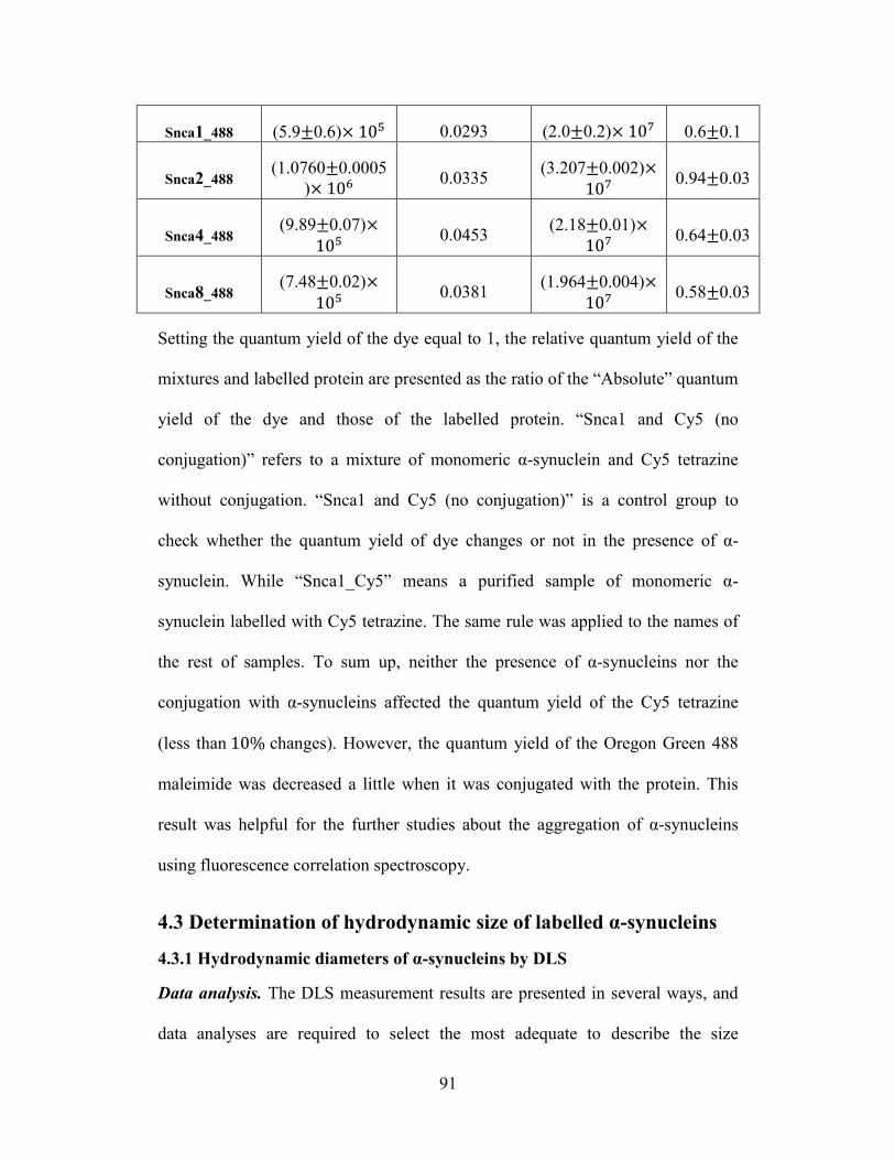
91
Snca1_488 (5.9±0.6)× 105 0.0293 (2.0±0.2)× 107 0.6±0.1
Snca2_488 (1.0760±0.0005
)× 106 0.0335
(3.207±0.002)×107
0.94±0.03
Snca4_488 (9.89±0.07)×
105 0.0453
(2.18±0.01)×107
0.64±0.03
Snca8_488 (7.48±0.02)×
105 0.0381
(1.964±0.004)×107
0.58±0.03
Setting the quantum yield of the dye equal to 1, the relative quantum yield of the
mixtures and labelled protein are presented as the ratio of the “Absolute” quantum
yield of the dye and those of the labelled protein. “Snca1 and Cy5 (no
conjugation)” refers to a mixture of monomeric α-synuclein and Cy5 tetrazine
without conjugation. “Snca1 and Cy5 (no conjugation)” is a control group to
check whether the quantum yield of dye changes or not in the presence of α-
synuclein. While “Snca1_Cy5” means a purified sample of monomeric α-
synuclein labelled with Cy5 tetrazine. The same rule was applied to the names of
the rest of samples. To sum up, neither the presence of α-synucleins nor the
conjugation with α-synucleins affected the quantum yield of the Cy5 tetrazine
(less than 10% changes). However, the quantum yield of the Oregon Green 488
maleimide was decreased a little when it was conjugated with the protein. This
result was helpful for the further studies about the aggregation of α-synucleins
using fluorescence correlation spectroscopy.
4.3 Determination of hydrodynamic size of labelled α-synucleins
4.3.1 Hydrodynamic diameters of α-synucleins by DLS
Data analysis. The DLS measurement results are presented in several ways, and
data analyses are required to select the most adequate to describe the size
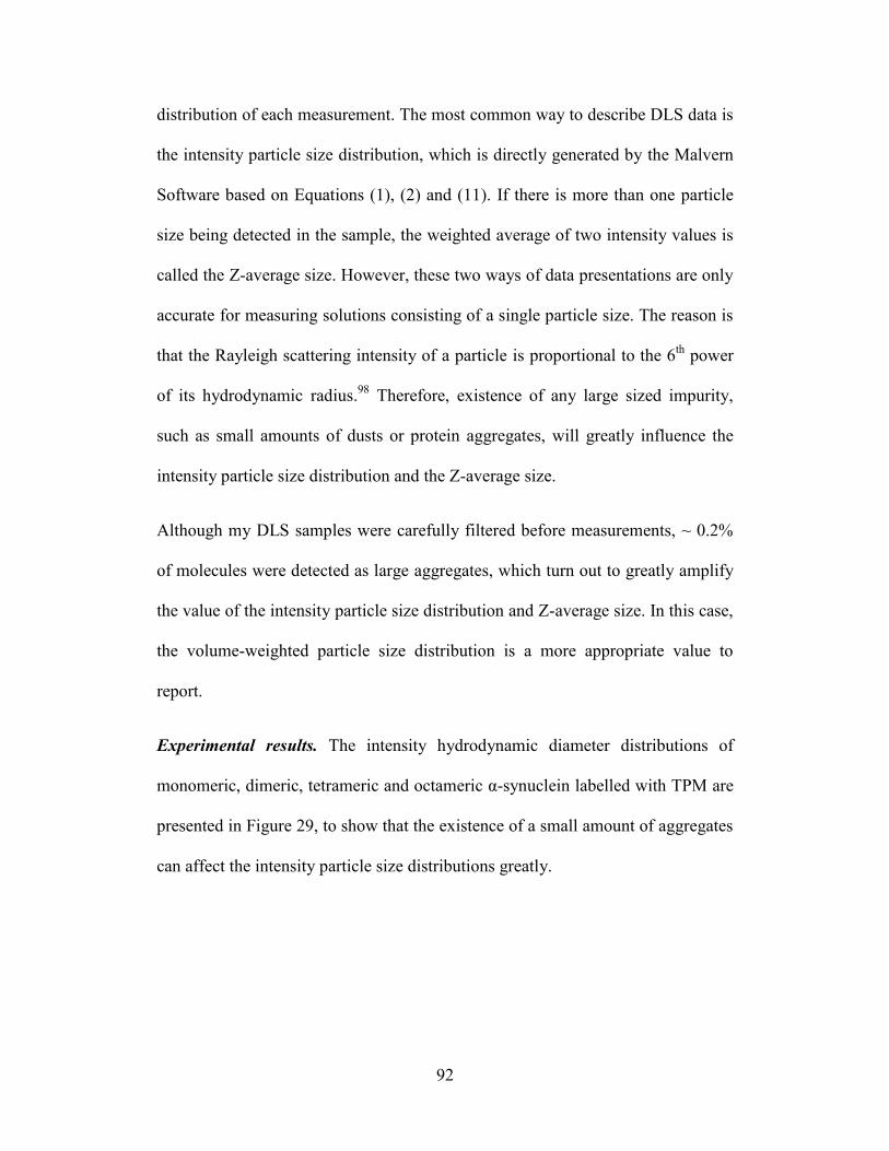
92
distribution of each measurement. The most common way to describe DLS data is
the intensity particle size distribution, which is directly generated by the Malvern
Software based on Equations (1), (2) and (11). If there is more than one particle
size being detected in the sample, the weighted average of two intensity values is
called the Z-average size. However, these two ways of data presentations are only
accurate for measuring solutions consisting of a single particle size. The reason is
that the Rayleigh scattering intensity of a particle is proportional to the 6th
power
of its hydrodynamic radius.98
Therefore, existence of any large sized impurity,
such as small amounts of dusts or protein aggregates, will greatly influence the
intensity particle size distribution and the Z-average size.
Although my DLS samples were carefully filtered before measurements, ~ 0.2%
of molecules were detected as large aggregates, which turn out to greatly amplify
the value of the intensity particle size distribution and Z-average size. In this case,
the volume-weighted particle size distribution is a more appropriate value to
report.
Experimental results. The intensity hydrodynamic diameter distributions of
monomeric, dimeric, tetrameric and octameric α-synuclein labelled with TPM are
presented in Figure 29, to show that the existence of a small amount of aggregates
can affect the intensity particle size distributions greatly.
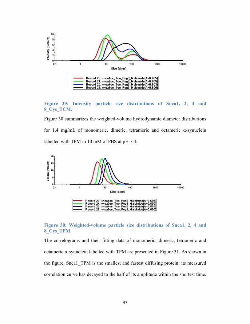
93
Figure 29: Intensity particle size distributions of Snca1, 2, 4 and
8_Cys_TCM.
Figure 30 summarizes the weighted-volume hydrodynamic diameter distributions
for 1.4 mg/mL of monomeric, dimeric, tetrameric and octameric α-synuclein
labelled with TPM in 10 mM of PBS at pH 7.4.
Figure 30: Weighted-volume particle size distributions of Snca1, 2, 4 and
8_Cys_TPM.
The correlograms and their fitting data of monomeric, dimeric, tetrameric and
octameric α-synuclein labelled with TPM are presented in Figure 31. As shown in
the figure, Snca1_TPM is the smallest and fastest diffusing protein; its measured
correlation curve has decayed to the half of its amplitude within the shortest time.
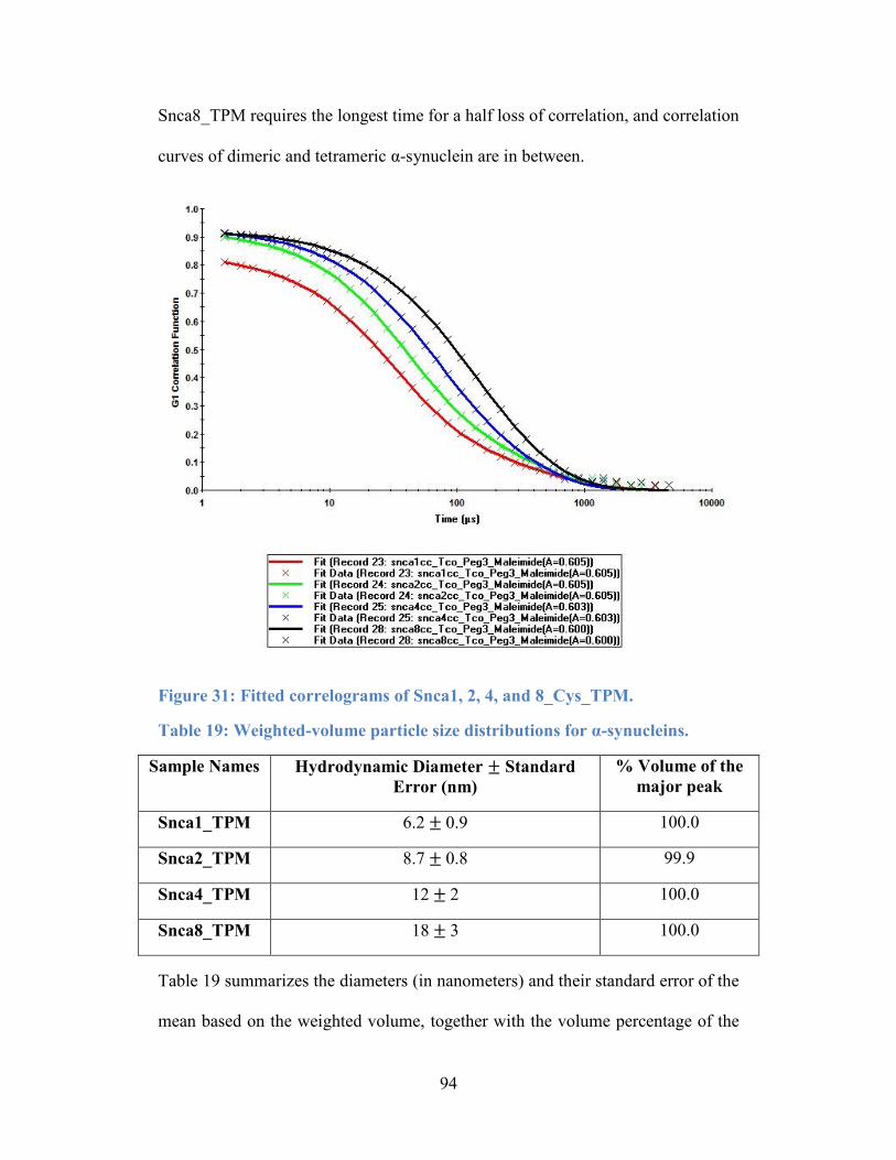
94
Snca8_TPM requires the longest time for a half loss of correlation, and correlation
curves of dimeric and tetrameric α-synuclein are in between.
Figure 31: Fitted correlograms of Snca1, 2, 4, and 8_Cys_TPM.
Table 19: Weighted-volume particle size distributions for α-synucleins.
Sample Names Hydrodynamic Diameter ± Standard
Error (nm)
% Volume of the
major peak
Snca1_TPM 6.2 ± 0.9 100.0
Snca2_TPM 8.7 ± 0.8 99.9
Snca4_TPM 12 ± 2 100.0
Snca8_TPM 18 ± 3 100.0
Table 19 summarizes the diameters (in nanometers) and their standard error of the
mean based on the weighted volume, together with the volume percentage of the
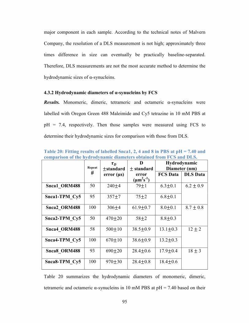
95
major component in each sample. According to the technical notes of Malvern
Company, the resolution of a DLS measurement is not high; approximately three
times difference in size can eventually be practically baseline-separated.
Therefore, DLS measurements are not the most accurate method to determine the
hydrodynamic sizes of α-synucleins.
4.3.2 Hydrodynamic diameters of α-synucleins by FCS
Results. Monomeric, dimeric, tetrameric and octameric α-synucleins were
labelled with Oregon Green 488 Maleimide and Cy5 tetrazine in 10 mM PBS at
pH = 7.4, respectively. Then those samples were measured using FCS to
determine their hydrodynamic sizes for comparison with those from DLS.
Table 20: Fitting results of labelled Snca1, 2, 4 and 8 in PBS at pH = 7.40 and
comparison of the hydrodynamic diameters obtained from FCS and DLS.
Repeat
#
𝝉𝑫
±standard
error (µs)
D
± standard
error
(μm2s
-1)
Hydrodynamic
Diameter (nm)
FCS Data DLS Data
Snca1_ORM488 50 240±4 79±1 6.3±0.1 6.2 ± 0.9
Snca1-TPM_Cy5 95 357±7 75±2 6.8±0.1
Snca2_ORM488 100 306±4 61.9±0.7 8.0±0.1 8.7 ± 0.8
Snca2-TPM_Cy5 50 470±20 58±2 8.8±0.3
Snca4_ORM488 58 500±10 38.5±0.9 13.1±0.3 12 ± 2
Snca4-TPM_Cy5 100 670±10 38.6±0.9 13.2±0.3
Snca8_ORM488 93 690±20 28.4±0.6 17.9±0.4 18 ± 3
Snca8-TPM_Cy5 100 970±30 28.4±0.8 18.4±0.6
Table 20 summarizes the hydrodynamic diameters of monomeric, dimeric,
tetrameric and octameric α-synucleins in 10 mM PBS at pH = 7.40 based on their
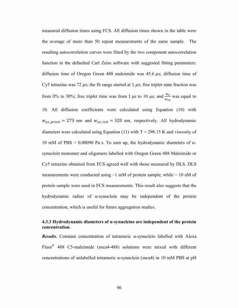
96
measured diffusion times using FCS. All diffusion times shown in the table were
the average of more than 50 repeat measurements of the same sample. The
resulting autocorrelation curves were fitted by the two component autocorrelation
function in the defaulted Carl Zeiss software with suggested fitting parameters:
diffusion time of Oregon Green 488 maleimide was 45.6 𝜇s; diffusion time of
Cy5 tetrazine was 72 𝜇s; the fit range started at 1 𝜇𝑠; free triplet state fraction was
from 0% to 30%; free triplet time was from 1 μ𝑠 to 10 μs; and 𝑤𝑧
𝑤𝑥𝑦 was equal to
10. All diffusion coefficients were calculated using Equation (10) with
𝑤𝑥𝑦_𝑔𝑟𝑒𝑒𝑛 = 273 nm and 𝑤𝑥𝑦_𝑟𝑒𝑑 = 320 nm, respectively. All hydrodynamic
diameters were calculated using Equation (11) with T = 298.15 K and viscosity of
10 mM of PBS = 0.00090 Pa·s. To sum up, the hydrodynamic diameters of α-
synuclein monomer and oligomers labelled with Oregon Green 488 Maleimide or
Cy5 tetrazine obtained from FCS agreed well with those measured by DLS. DLS
measurements were conducted using ~1 mM of protein sample, while ~ 10 nM of
protein sample were used in FCS measurements. This result also suggests that the
hydrodynamic radius of α-synuclein may be independent of the protein
concentration, which is useful for future aggregation studies.
4.3.3 Hydrodynamic diameters of α-synucleins are independent of the protein
concentration.
Results. Constant concentration of tetrameric α-synuclein labelled with Alexa
Fluor® 488 C5-maleimide (snca4-488) solutions were mixed with different
concentrations of unlabelled tetrameric α-synuclein (snca4) in 10 mM PBS at pH
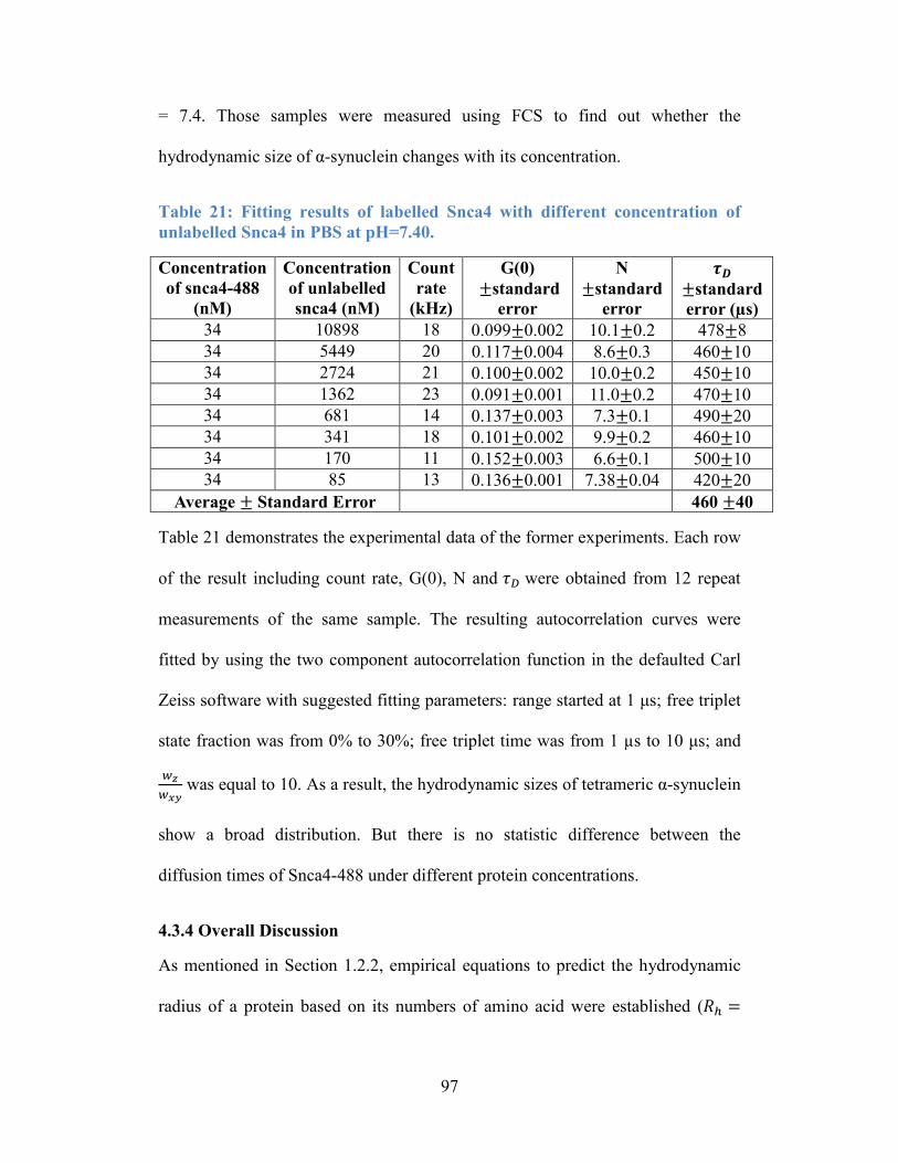
97
= 7.4. Those samples were measured using FCS to find out whether the
hydrodynamic size of α-synuclein changes with its concentration.
Table 21: Fitting results of labelled Snca4 with different concentration of
unlabelled Snca4 in PBS at pH=7.40.
Concentration
of snca4-488
(nM)
Concentration
of unlabelled
snca4 (nM)
Count
rate
(kHz)
G(0)
±standard
error
N
±standard
error
𝝉𝑫
±standard
error (µs)
34 10898 18 0.099±0.002 10.1±0.2 478±8
34 5449 20 0.117±0.004 8.6±0.3 460±10
34 2724 21 0.100±0.002 10.0±0.2 450±10
34 1362 23 0.091±0.001 11.0±0.2 470±10
34 681 14 0.137±0.003 7.3±0.1 490±20
34 341 18 0.101±0.002 9.9±0.2 460±10
34 170 11 0.152±0.003 6.6±0.1 500±10
34 85 13 0.136±0.001 7.38±0.04 420±20
Average ± Standard Error 460 ±40
Table 21 demonstrates the experimental data of the former experiments. Each row
of the result including count rate, G(0), N and 𝜏𝐷 were obtained from 12 repeat
measurements of the same sample. The resulting autocorrelation curves were
fitted by using the two component autocorrelation function in the defaulted Carl
Zeiss software with suggested fitting parameters: range started at 1 μs; free triplet
state fraction was from 0% to 30%; free triplet time was from 1 µs to 10 μs; and
𝑤𝑧
𝑤𝑥𝑦 was equal to 10. As a result, the hydrodynamic sizes of tetrameric α-synuclein
show a broad distribution. But there is no statistic difference between the
diffusion times of Snca4-488 under different protein concentrations.
4.3.4 Overall Discussion
As mentioned in Section 1.2.2, empirical equations to predict the hydrodynamic
radius of a protein based on its numbers of amino acid were established (𝑅ℎ =
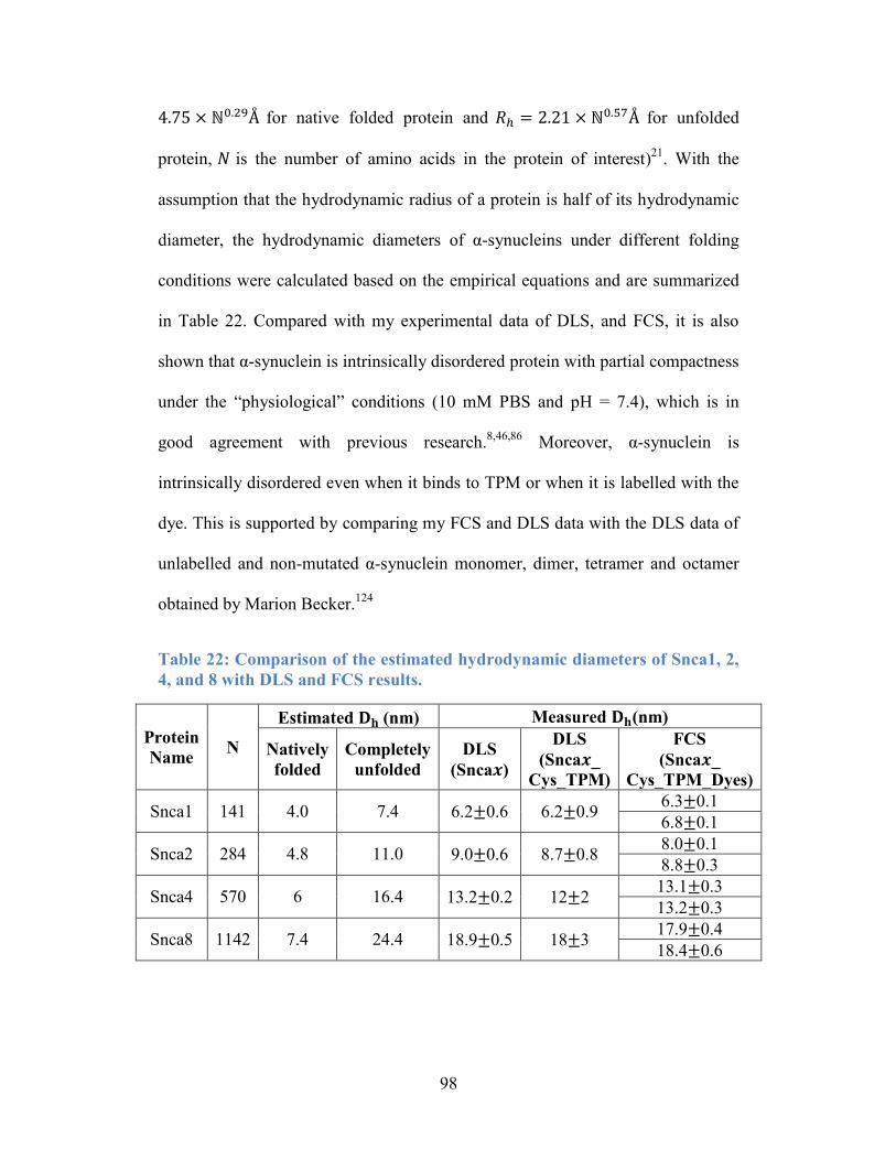
98
4.75 × ℕ0.29Å for native folded protein and 𝑅ℎ = 2.21 × ℕ0.57Å for unfolded
protein, 𝑁 is the number of amino acids in the protein of interest)21
. With the
assumption that the hydrodynamic radius of a protein is half of its hydrodynamic
diameter, the hydrodynamic diameters of α-synucleins under different folding
conditions were calculated based on the empirical equations and are summarized
in Table 22. Compared with my experimental data of DLS, and FCS, it is also
shown that α-synuclein is intrinsically disordered protein with partial compactness
under the “physiological” conditions (10 mM PBS and pH = 7.4), which is in
good agreement with previous research.8,46,86
Moreover, α-synuclein is
intrinsically disordered even when it binds to TPM or when it is labelled with the
dye. This is supported by comparing my FCS and DLS data with the DLS data of
unlabelled and non-mutated α-synuclein monomer, dimer, tetramer and octamer
obtained by Marion Becker.124
Table 22: Comparison of the estimated hydrodynamic diameters of Snca1, 2,
4, and 8 with DLS and FCS results.
Protein
Name N
Estimated 𝐃𝐡 (nm) Measured 𝐃𝐡(nm)
Natively
folded
Completely
unfolded
DLS
(Snca𝒙)
DLS
(Snca𝒙_
Cys_TPM)
FCS
(Snca𝒙_
Cys_TPM_Dyes)
Snca1 141 4.0 7.4 6.2±0.6 6.2±0.9 6.3±0.1
6.8±0.1
Snca2 284 4.8 11.0 9.0±0.6 8.7±0.8 8.0±0.1
8.8±0.3
Snca4 570 6 16.4 13.2±0.2 12±2 13.1±0.3
13.2±0.3
Snca8 1142 7.4 24.4 18.9±0.5 18±3 17.9±0.4
18.4±0.6
99
4.4 Aggregation of labelled α-synucleins
4.4.1 Aggregation tests by FCS
In the first aggregation experiment, a small amount of labelled α-synucleins and a
large excess of unlabelled α-synucleins were incubated together, and the mixture
was measured by FCS to determine whether the diffusion of the labelled protein
would change if aggregation occurred. Figure 32 (a) displays the distributions of
the measured diffusion time of a sample which contains ~ 0.3 μM of labelled
monomeric α-synuclein and 150 μM unlabelled monomer over 120 hours. There
is no apparent change in the distribution of diffusion times after the sample was
incubated at 310.15 K for 120 hours with continuous shaking at 250 rpm. Figure
32 (b) displays the distributions of the measured diffusion time of a sample which
contained ~ 0.03 μM of labelled tetrameric α-synuclein and 10 μM of unlabelled
tetrameric protein at incubation times over 6 hours. No change in distribution is
discovered, although there are a few outliers of very large diffusion times after 0.4
hours.
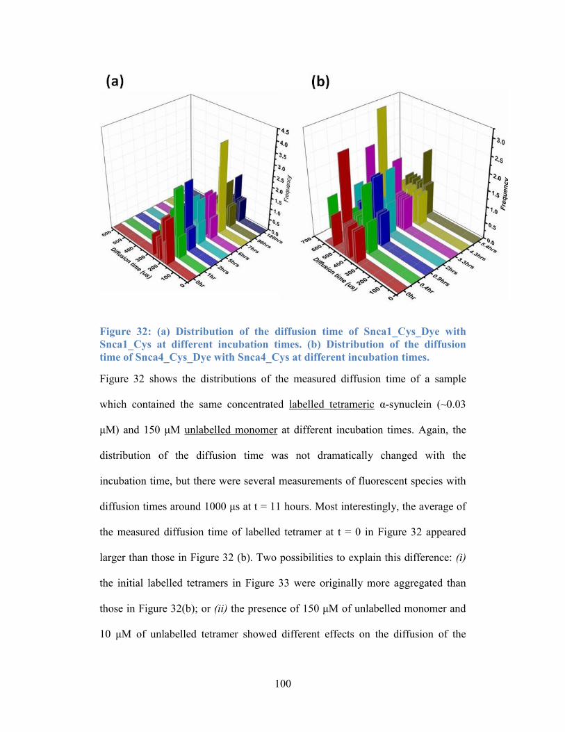
100
Figure 32: (a) Distribution of the diffusion time of Snca1_Cys_Dye with
Snca1_Cys at different incubation times. (b) Distribution of the diffusion
time of Snca4_Cys_Dye with Snca4_Cys at different incubation times.
Figure 32 shows the distributions of the measured diffusion time of a sample
which contained the same concentrated labelled tetrameric α-synuclein (~0.03
μM) and 150 μM unlabelled monomer at different incubation times. Again, the
distribution of the diffusion time was not dramatically changed with the
incubation time, but there were several measurements of fluorescent species with
diffusion times around 1000 μs at t = 11 hours. Most interestingly, the average of
the measured diffusion time of labelled tetramer at t = 0 in Figure 32 appeared
larger than those in Figure 32 (b). Two possibilities to explain this difference: (i)
the initial labelled tetramers in Figure 33 were originally more aggregated than
those in Figure 32(b); or (ii) the presence of 150 μM of unlabelled monomer and
10 μM of unlabelled tetramer showed different effects on the diffusion of the
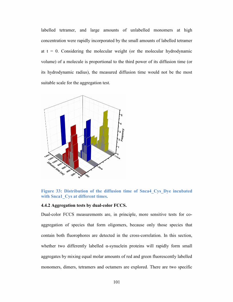
101
labelled tetramer, and large amounts of unlabelled monomers at high
concentration were rapidly incorporated by the small amounts of labelled tetramer
at t = 0. Considering the molecular weight (or the molecular hydrodynamic
volume) of a molecule is proportional to the third power of its diffusion time (or
its hydrodynamic radius), the measured diffusion time would not be the most
suitable scale for the aggregation test.
Figure 33: Distribution of the diffusion time of Snca4_Cys_Dye incubated
with Snca1_Cys at different times.
4.4.2 Aggregation tests by dual-color FCCS.
Dual-color FCCS measurements are, in principle, more sensitive tests for co-
aggregation of species that form oligomers, because only those species that
contain both fluorophores are detected in the cross-correlation. In this section,
whether two differently labelled α-synuclein proteins will rapidly form small
aggregates by mixing equal molar amounts of red and green fluorescently labelled
monomers, dimers, tetramers and octamers are explored. There are two specific
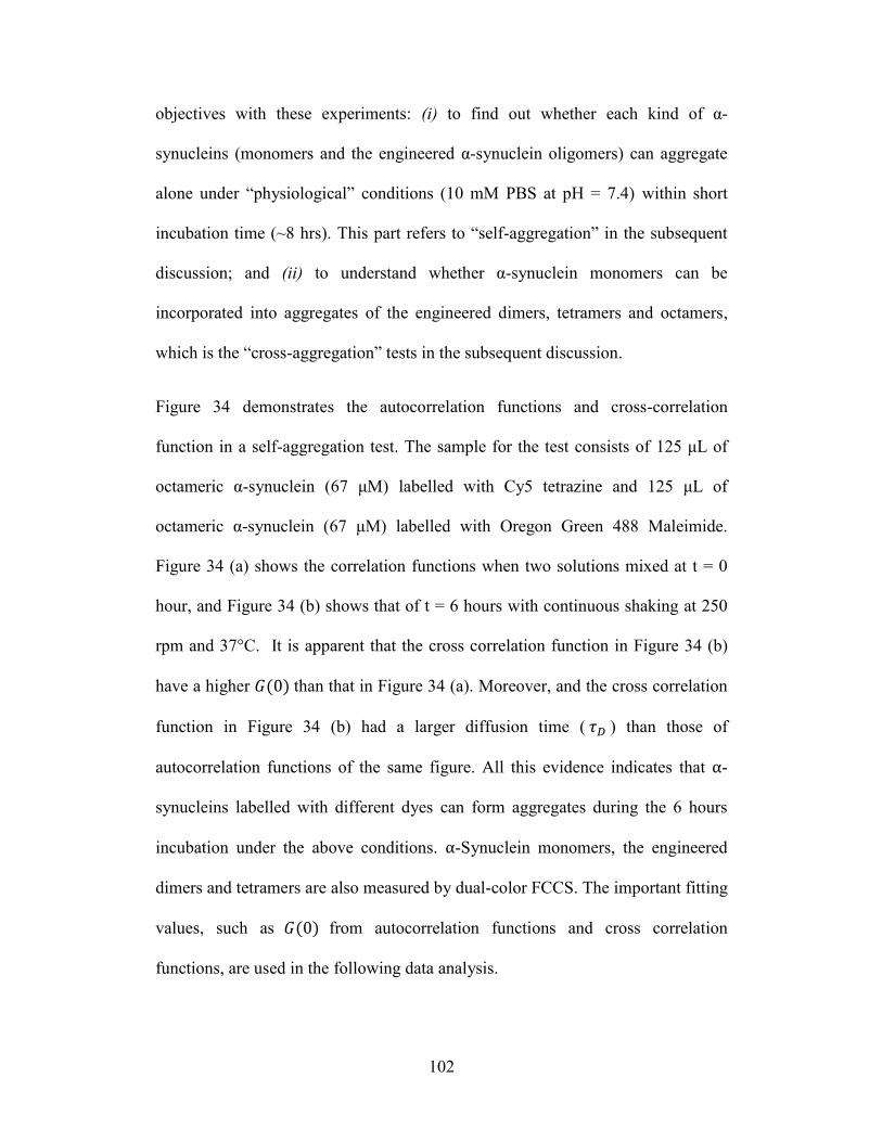
102
objectives with these experiments: (i) to find out whether each kind of α-
synucleins (monomers and the engineered α-synuclein oligomers) can aggregate
alone under “physiological” conditions (10 mM PBS at pH = 7.4) within short
incubation time (~8 hrs). This part refers to “self-aggregation” in the subsequent
discussion; and (ii) to understand whether α-synuclein monomers can be
incorporated into aggregates of the engineered dimers, tetramers and octamers,
which is the “cross-aggregation” tests in the subsequent discussion.
Figure 34 demonstrates the autocorrelation functions and cross-correlation
function in a self-aggregation test. The sample for the test consists of 125 μL of
octameric α-synuclein (67 μM) labelled with Cy5 tetrazine and 125 μL of
octameric α-synuclein (67 μM) labelled with Oregon Green 488 Maleimide.
Figure 34 (a) shows the correlation functions when two solutions mixed at t = 0
hour, and Figure 34 (b) shows that of t = 6 hours with continuous shaking at 250
rpm and 37°C. It is apparent that the cross correlation function in Figure 34 (b)
have a higher 𝐺(0) than that in Figure 34 (a). Moreover, and the cross correlation
function in Figure 34 (b) had a larger diffusion time ( 𝜏𝐷 ) than those of
autocorrelation functions of the same figure. All this evidence indicates that α-
synucleins labelled with different dyes can form aggregates during the 6 hours
incubation under the above conditions. α-Synuclein monomers, the engineered
dimers and tetramers are also measured by dual-color FCCS. The important fitting
values, such as 𝐺(0) from autocorrelation functions and cross correlation
functions, are used in the following data analysis.
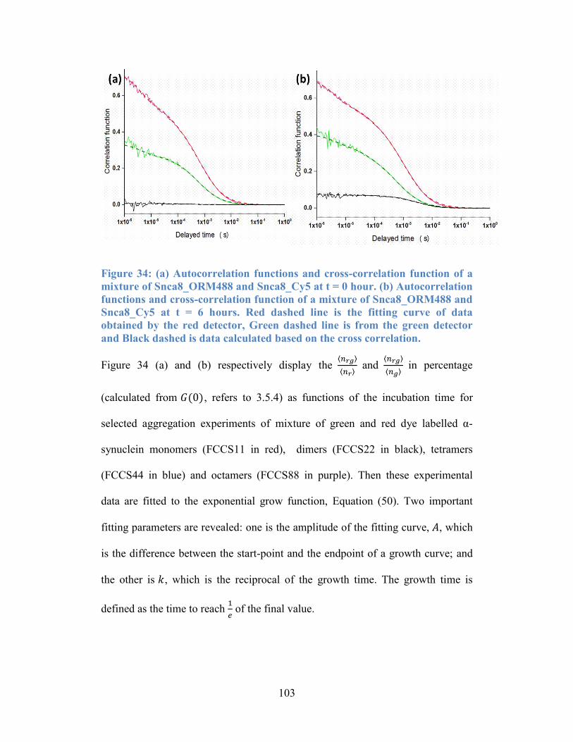
103
Figure 34: (a) Autocorrelation functions and cross-correlation function of a
mixture of Snca8_ORM488 and Snca8_Cy5 at t = 0 hour. (b) Autocorrelation
functions and cross-correlation function of a mixture of Snca8_ORM488 and
Snca8_Cy5 at t = 6 hours. Red dashed line is the fitting curve of data
obtained by the red detector, Green dashed line is from the green detector
and Black dashed is data calculated based on the cross correlation.
Figure 34 (a) and (b) respectively display the ⟨𝑛𝑟𝑔⟩
⟨𝑛𝑟⟩ and
⟨𝑛𝑟𝑔⟩
⟨𝑛𝑔⟩ in percentage
(calculated from 𝐺(0), refers to 3.5.4) as functions of the incubation time for
selected aggregation experiments of mixture of green and red dye labelled α-
synuclein monomers (FCCS11 in red), dimers (FCCS22 in black), tetramers
(FCCS44 in blue) and octamers (FCCS88 in purple). Then these experimental
data are fitted to the exponential grow function, Equation (50). Two important
fitting parameters are revealed: one is the amplitude of the fitting curve, 𝐴, which
is the difference between the start-point and the endpoint of a growth curve; and
the other is 𝑘, which is the reciprocal of the growth time. The growth time is
defined as the time to reach 1
𝑒 of the final value.
104
Figure 35: (a) ⟨𝐧𝐫𝐠⟩
⟨𝐧𝐫⟩ as a function of incubation time; (b)
⟨𝐧𝐫𝐠⟩
⟨𝐧𝐠⟩as a function of
incubation time for FCCS 11 (red), FCCS 22 (black), FCCS 44 (blue) and
FCCS 88 (purple).
Self-aggregation: Analysis of the amplitude of fitting curves. It was evident from
Figure 35 (a) that the extent and the rate of increase of the FCCS 88 fractions
were the largest while those of the FCCS 11 were the smallest, and those of FCCS
22 and 44 were in between. Figure 35 (b) shows an overall similar trend, but with
relatively smaller changes in these fractions. This indicates that more red dye
labelled α-synuclein is incorporated into the aggregates than the green dye
labelled α-synuclein. Moreover, it is interesting to point out that the extent and the
rate of the FCCS 44 aggregation curve are larger than those of the FCCS 88 in
Figure 35 (b).
Table 23 summarizes the amplitude (in %) with its standard error of the fitting
curves of all FCCS self-aggregation experiments. Each test reveals the average
amplitude of 50 repeated measurements of the same sample. Same test is repeated
3~4 times and newly prepared samples are used each time. Finally the average
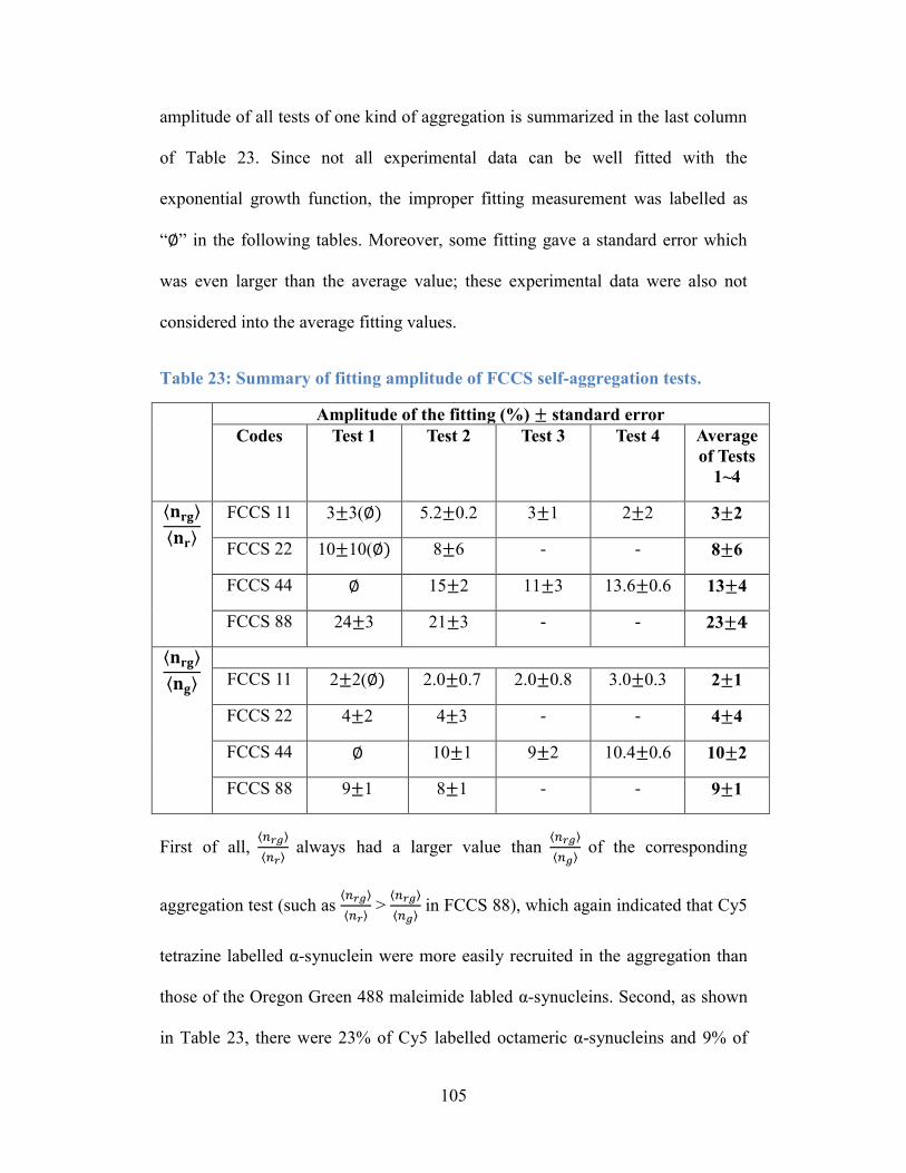
105
amplitude of all tests of one kind of aggregation is summarized in the last column
of Table 23. Since not all experimental data can be well fitted with the
exponential growth function, the improper fitting measurement was labelled as
“∅” in the following tables. Moreover, some fitting gave a standard error which
was even larger than the average value; these experimental data were also not
considered into the average fitting values.
Table 23: Summary of fitting amplitude of FCCS self-aggregation tests.
Amplitude of the fitting (%) ± standard error
Codes Test 1 Test 2 Test 3 Test 4 Average
of Tests
1~4
⟨𝐧𝐫𝐠⟩
⟨𝐧𝐫⟩
FCCS 11 3±3(∅) 5.2±0.2 3±1 2±2 3±2
FCCS 22 10±10(∅) 8±6 - - 8±6
FCCS 44 ∅ 15±2 11±3 13.6±0.6 13±4
FCCS 88 24±3 21±3 - - 23±𝟒
⟨𝐧𝐫𝐠⟩
⟨𝐧𝐠⟩
FCCS 11 2±2(∅) 2.0±0.7 2.0±0.8 3.0±0.3 2±1
FCCS 22 4±2 4±3 - - 4±4
FCCS 44 ∅ 10±1 9±2 10.4±0.6 10±2
FCCS 88 9±1 8±1 - - 9±1
First of all, ⟨𝑛𝑟𝑔⟩
⟨𝑛𝑟⟩ always had a larger value than
⟨𝑛𝑟𝑔⟩
⟨𝑛𝑔⟩ of the corresponding
aggregation test (such as ⟨𝑛𝑟𝑔⟩
⟨𝑛𝑟⟩ >
⟨𝑛𝑟𝑔⟩
⟨𝑛𝑔⟩ in FCCS 88), which again indicated that Cy5
tetrazine labelled α-synuclein were more easily recruited in the aggregation than
those of the Oregon Green 488 maleimide labled α-synucleins. Second, as shown
in Table 23, there were 23% of Cy5 labelled octameric α-synucleins and 9% of
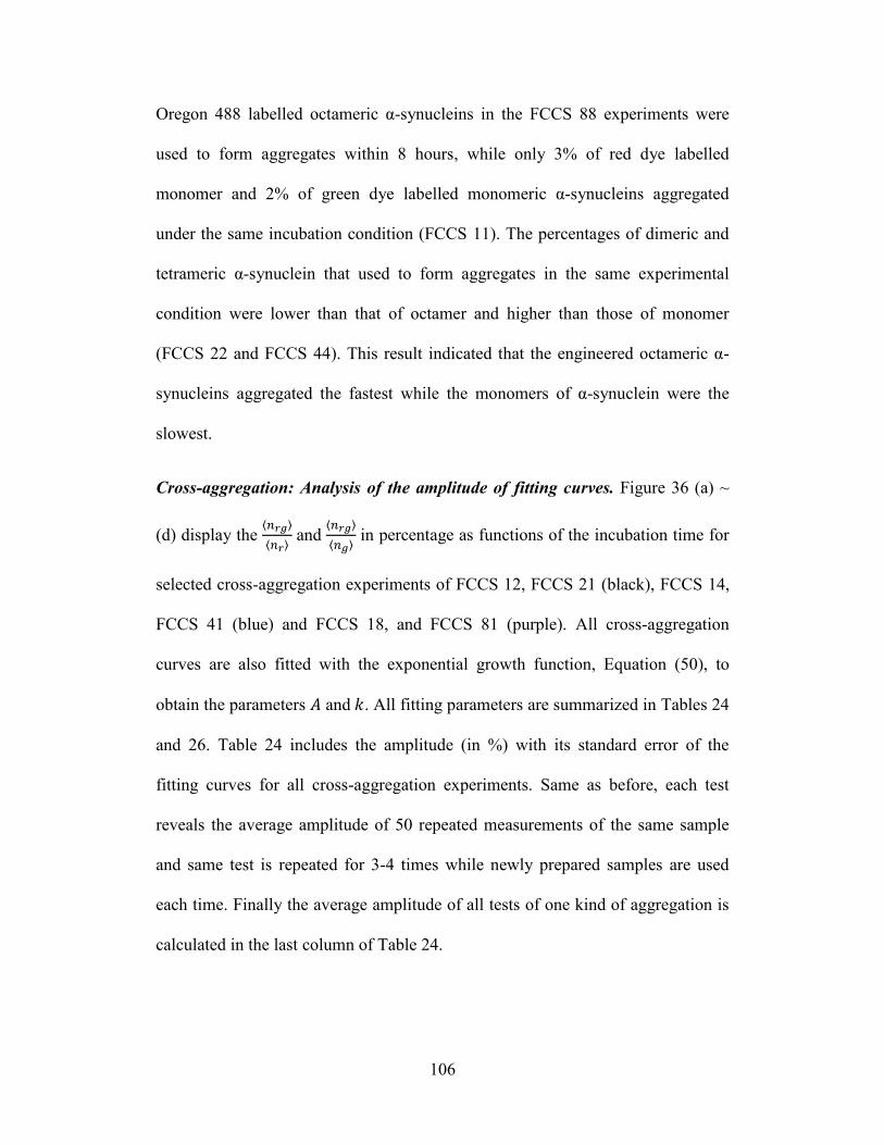
106
Oregon 488 labelled octameric α-synucleins in the FCCS 88 experiments were
used to form aggregates within 8 hours, while only 3% of red dye labelled
monomer and 2% of green dye labelled monomeric α-synucleins aggregated
under the same incubation condition (FCCS 11). The percentages of dimeric and
tetrameric α-synuclein that used to form aggregates in the same experimental
condition were lower than that of octamer and higher than those of monomer
(FCCS 22 and FCCS 44). This result indicated that the engineered octameric α-
synucleins aggregated the fastest while the monomers of α-synuclein were the
slowest.
Cross-aggregation: Analysis of the amplitude of fitting curves. Figure 36 (a) ~
(d) display the ⟨𝑛𝑟𝑔⟩
⟨𝑛𝑟⟩ and
⟨𝑛𝑟𝑔⟩
⟨𝑛𝑔⟩ in percentage as functions of the incubation time for
selected cross-aggregation experiments of FCCS 12, FCCS 21 (black), FCCS 14,
FCCS 41 (blue) and FCCS 18, and FCCS 81 (purple). All cross-aggregation
curves are also fitted with the exponential growth function, Equation (50), to
obtain the parameters 𝐴 and 𝑘. All fitting parameters are summarized in Tables 24
and 26. Table 24 includes the amplitude (in %) with its standard error of the
fitting curves for all cross-aggregation experiments. Same as before, each test
reveals the average amplitude of 50 repeated measurements of the same sample
and same test is repeated for 3-4 times while newly prepared samples are used
each time. Finally the average amplitude of all tests of one kind of aggregation is
calculated in the last column of Table 24.
107
Figure 36: (a) ⟨𝒏𝒓𝒈⟩
⟨𝒏𝒓⟩ as a function of incubation time for FCCS 12, 14 and 18;
(b) ⟨𝒏𝒓𝒈⟩
⟨𝒏𝒈⟩ as a function of incubation time for for FCCS 12, 14 and 18; (c)
⟨𝒏𝒓𝒈⟩
⟨𝒏𝒓⟩ as a function of incubation time for FCCS 21, 41 and 81; (d)
⟨𝒏𝒓𝒈⟩
⟨𝒏𝒈⟩ as a
function of incubation time for FCCS 21, 41 and 81. Black for sample
contained dimeric α-synuclein, blue for tetramers and purple for octamers.
As shown in both Figure 36 and Table 24, the engineered α-synuclein dimer,
tetramer and octamer preferred to incorporate itself than monomer to the
aggregation process when the same protein concentration monomer and oligomer
solutions were mixed within 8 hour incubations. It concluded based on the fact
that only 0.9 ~ 3% of red dye labelled monomeric α-synuclein (⟨𝑛𝑟𝑔⟩
⟨𝑛𝑟⟩ of FCCS 12,
14 and 18 or Figure 36 (a)) were enrolled in the aggregation while 5-11% of green
labelled oligomers (⟨𝑛𝑟𝑔⟩
⟨𝑛𝑔⟩ of FCCS 12, 14 and 18 or Figure 36 (b)) were used in the
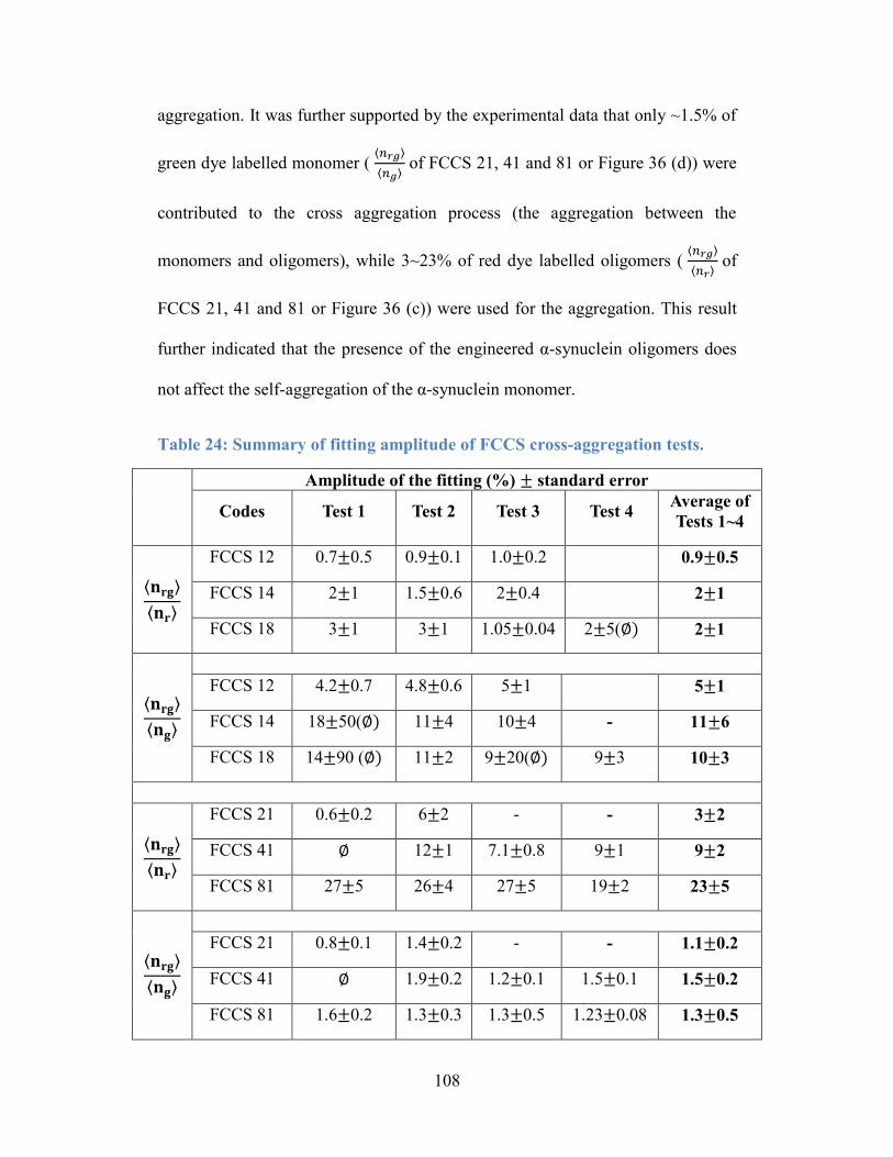
108
aggregation. It was further supported by the experimental data that only ~1.5% of
green dye labelled monomer ( ⟨𝑛𝑟𝑔⟩
⟨𝑛𝑔⟩ of FCCS 21, 41 and 81 or Figure 36 (d)) were
contributed to the cross aggregation process (the aggregation between the
monomers and oligomers), while 3~23% of red dye labelled oligomers ( ⟨𝑛𝑟𝑔⟩
⟨𝑛𝑟⟩ of
FCCS 21, 41 and 81 or Figure 36 (c)) were used for the aggregation. This result
further indicated that the presence of the engineered α-synuclein oligomers does
not affect the self-aggregation of the α-synuclein monomer.
Table 24: Summary of fitting amplitude of FCCS cross-aggregation tests.
Amplitude of the fitting (%) ± standard error
Codes Test 1 Test 2 Test 3 Test 4 Average of
Tests 1~4
⟨𝐧𝐫𝐠⟩
⟨𝐧𝐫⟩
FCCS 12 0.7±0.5 0.9±0.1 1.0±0.2 0.9±0.5
FCCS 14 2±1 1.5±0.6 2±0.4 2±1
FCCS 18 3±1 3±1 1.05±0.04 2±5(∅) 2±1
⟨𝐧𝐫𝐠⟩
⟨𝐧𝐠⟩
FCCS 12 4.2±0.7 4.8±0.6 5±1 5±1
FCCS 14 18±50(∅) 11±4 10±4 - 11±6
FCCS 18 14±90 (∅) 11±2 9±20(∅) 9±3 10±3
⟨𝐧𝐫𝐠⟩
⟨𝐧𝐫⟩
FCCS 21 0.6±0.2 6±2 - - 3±2
FCCS 41 ∅ 12±1 7.1±0.8 9±1 9±2
FCCS 81 27±5 26±4 27±5 19±2 23±5
⟨𝐧𝐫𝐠⟩
⟨𝐧𝐠⟩
FCCS 21 0.8±0.1 1.4±0.2 - - 1.1±0.2
FCCS 41 ∅ 1.9±0.2 1.2±0.1 1.5±0.1 1.5±0.2
FCCS 81 1.6±0.2 1.3±0.3 1.3±0.5 1.23±0.08 1.3±0.5
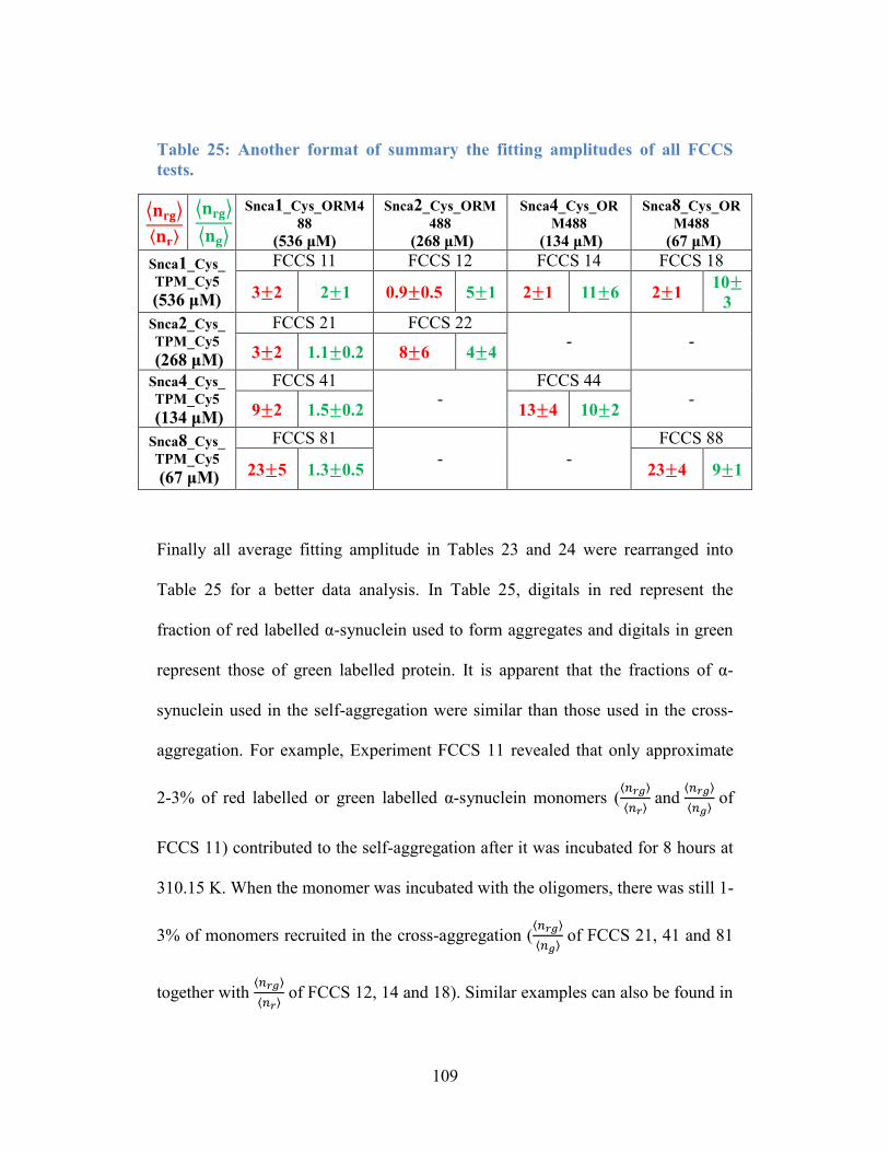
109
Table 25: Another format of summary the fitting amplitudes of all FCCS
tests.
⟨𝐧𝐫𝐠⟩
⟨𝐧𝐫⟩
⟨𝐧𝐫𝐠⟩
⟨𝐧𝐠⟩
Snca1_Cys_ORM4
88
(536 μM)
Snca2_Cys_ORM
488
(268 μM)
Snca4_Cys_OR
M488
(134 μM)
Snca8_Cys_OR
M488
(67 μM)
Snca1_Cys_
TPM_Cy5
(536 μM)
FCCS 11 FCCS 12 FCCS 14 FCCS 18
3±2 2±1 0.9±0.5 5±1 2±1 11±6 2±1 10±
3
Snca2_Cys_
TPM_Cy5
(268 μM)
FCCS 21 FCCS 22 - -
3±2 1.1±0.2 8±6 4±4
Snca4_Cys_
TPM_Cy5
(134 μM)
FCCS 41 -
FCCS 44 -
9±2 1.5±0.2 13±4 10±2
Snca8_Cys_
TPM_Cy5
(67 μM)
FCCS 81
- -
FCCS 88
23±5 1.3±0.5 23±4 9±1
Finally all average fitting amplitude in Tables 23 and 24 were rearranged into
Table 25 for a better data analysis. In Table 25, digitals in red represent the
fraction of red labelled α-synuclein used to form aggregates and digitals in green
represent those of green labelled protein. It is apparent that the fractions of α-
synuclein used in the self-aggregation were similar than those used in the cross-
aggregation. For example, Experiment FCCS 11 revealed that only approximate
2-3% of red labelled or green labelled α-synuclein monomers (⟨𝑛𝑟𝑔⟩
⟨𝑛𝑟⟩ and
⟨𝑛𝑟𝑔⟩
⟨𝑛𝑔⟩ of
FCCS 11) contributed to the self-aggregation after it was incubated for 8 hours at
310.15 K. When the monomer was incubated with the oligomers, there was still 1-
3% of monomers recruited in the cross-aggregation (⟨𝑛𝑟𝑔⟩
⟨𝑛𝑔⟩ of FCCS 21, 41 and 81
together with ⟨𝑛𝑟𝑔⟩
⟨𝑛𝑟⟩ of FCCS 12, 14 and 18). Similar examples can also be found in
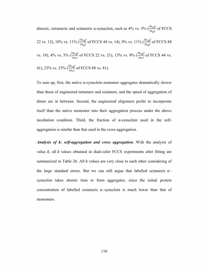
110
dimeric, tetrameric and octameric α-synuclein, such as 4% vs. 5% (⟨𝑛𝑟𝑔⟩
⟨𝑛𝑔⟩ of FCCS
22 vs. 12), 10% vs. 11% (⟨𝑛𝑟𝑔⟩
⟨𝑛𝑔⟩ of FCCS 44 vs. 14), 9% vs. 11% (
⟨𝑛𝑟𝑔⟩
⟨𝑛𝑔⟩ of FCCS 88
vs. 18), 4% vs. 3% (⟨𝑛𝑟𝑔⟩
⟨𝑛𝑟⟩ of FCCS 22 vs. 21), 13% vs. 9% (
⟨𝑛𝑟𝑔⟩
⟨𝑛𝑟⟩ of FCCS 44 vs.
41), 23% vs. 23% (⟨𝑛𝑟𝑔⟩
⟨𝑛𝑟⟩ of FCCS 88 vs. 81).
To sum up, first, the native α-synuclein monomer aggregates dramatically slower
than those of engineered tetramers and octamers, and the speed of aggregation of
dimer are in between. Second, the engineered oligomers prefer to incorporate
itself than the native monomer into their aggregation process under the above
incubation condition. Third, the fraction of α-synuclein used in the self-
aggregation is similar than that used in the cross-aggregation.
Analysis of k: self-aggregation and cross aggregation. With the analysis of
value 𝐴, all 𝑘 values obtained in dual-color FCCS experiments after fitting are
summarized in Table 26. All 𝑘 values are very close to each other considering of
the large standard errors. But we can still argue that labelled octameric 𝛼 -
synuclein takes shorter time to form aggregates, since the initial protein
concentration of labelled octameric 𝛼 -synuclein is much lower than that of
monomers.
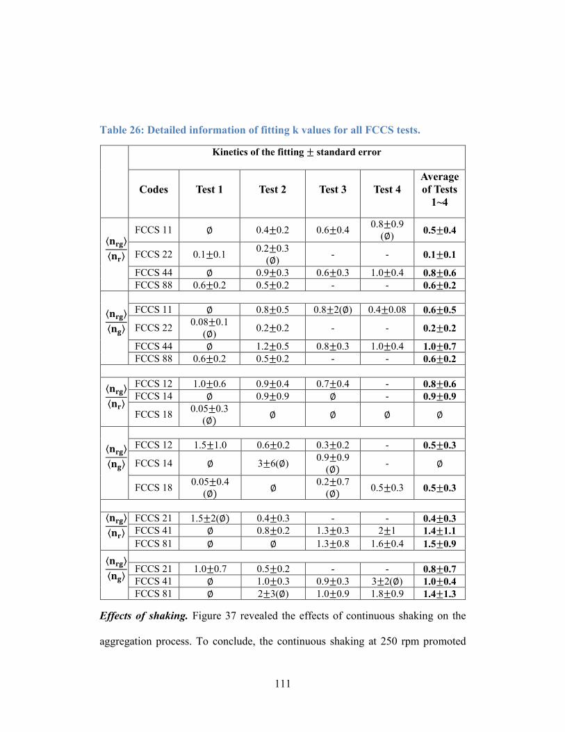
111
Table 26: Detailed information of fitting k values for all FCCS tests.
Kinetics of the fitting ± standard error
Codes Test 1 Test 2 Test 3 Test 4
Average
of Tests
1~4
⟨𝐧𝐫𝐠⟩
⟨𝐧𝐫⟩
FCCS 11 ∅ 0.4±0.2 0.6±0.4 0.8±0.9
(∅) 0.5±0.4
FCCS 22 0.1±0.1 0.2±0.3
(∅) - - 0.1±0.1
FCCS 44 ∅ 0.9±0.3 0.6±0.3 1.0±0.4 0.8±0.6
FCCS 88 0.6±0.2 0.5±0.2 - - 0.6±0.2
⟨𝐧𝐫𝐠⟩
⟨𝐧𝐠⟩
FCCS 11 ∅ 0.8±0.5 0.8±2(∅) 0.4±0.08 0.6±0.5
FCCS 22 0.08±0.1
(∅) 0.2±0.2 - - 0.2±0.2
FCCS 44 ∅ 1.2±0.5 0.8±0.3 1.0±0.4 1.0±0.7
FCCS 88 0.6±0.2 0.5±0.2 - - 0.6±0.2
⟨𝐧𝐫𝐠⟩
⟨𝐧𝐫⟩
FCCS 12 1.0±0.6 0.9±0.4 0.7±0.4 - 0.8±0.6
FCCS 14 ∅ 0.9±0.9 ∅ - 0.9±0.9
FCCS 18 0.05±0.3
(∅) ∅ ∅ ∅ ∅
⟨𝐧𝐫𝐠⟩
⟨𝐧𝐠⟩
FCCS 12 1.5±1.0 0.6±0.2 0.3±0.2 - 0.5±0.3
FCCS 14 ∅ 3±6(∅) 0.9±0.9
(∅) - ∅
FCCS 18 0.05±0.4
(∅) ∅
0.2±0.7
(∅) 0.5±0.3 0.5±0.3
⟨𝐧𝐫𝐠⟩
⟨𝐧𝐫⟩
FCCS 21 1.5±2(∅) 0.4±0.3 - - 0.4±0.3
FCCS 41 ∅ 0.8±0.2 1.3±0.3 2±1 1.4±1.1
FCCS 81 ∅ ∅ 1.3±0.8 1.6±0.4 1.5±0.9
⟨𝐧𝐫𝐠⟩
⟨𝐧𝐠⟩
FCCS 21 1.0±0.7 0.5±0.2 - - 0.8±0.7
FCCS 41 ∅ 1.0±0.3 0.9±0.3 3±2(∅) 1.0±0.4
FCCS 81 ∅ 2±3(∅) 1.0±0.9 1.8±0.9 1.4±1.3
Effects of shaking. Figure 37 revealed the effects of continuous shaking on the
aggregation process. To conclude, the continuous shaking at 250 rpm promoted
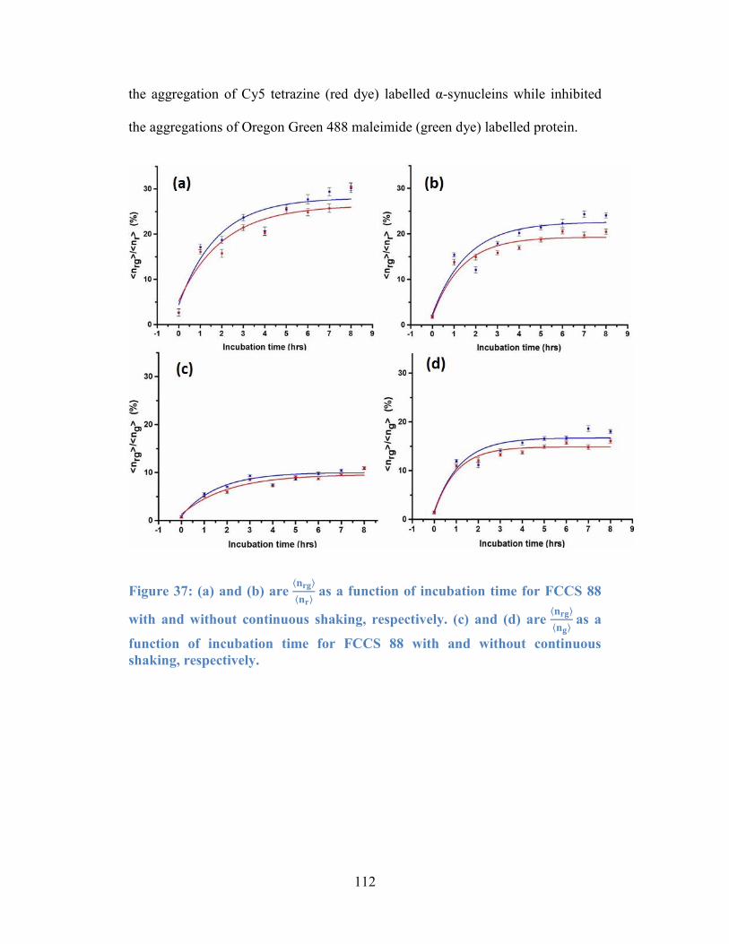
112
the aggregation of Cy5 tetrazine (red dye) labelled α-synucleins while inhibited
the aggregations of Oregon Green 488 maleimide (green dye) labelled protein.
Figure 37: (a) and (b) are ⟨𝐧𝐫𝐠⟩
⟨𝐧𝐫⟩ as a function of incubation time for FCCS 88
with and without continuous shaking, respectively. (c) and (d) are ⟨𝐧𝐫𝐠⟩
⟨𝐧𝐠⟩ as a
function of incubation time for FCCS 88 with and without continuous
shaking, respectively.
113
Chapter 5: Conclusion
5.1 Research summary and contributions
α-Synucleins exist in the neurons of the human brain. It promotes the functions of
neurons.57–61
It is believed that specific α-synuclein oligomers play an important
role of catalyzing the aggregation of normal monomeric α-synucleins, which
eventually cause the irreversible damages on the neurons. Therefore, we
constructed the engineered α-synuclein dimer, tetramer and octamer and studied
them using a variety of analytical methods including HPLC-MS, DLS, FCS and
dual-color FCCS. We measured the hydrodynamic diameters of all engineered α-
synucleins using both DLS and FCS. Both experimental data agreed well. These
data enable us to deduce that these engineered α-synucleins are not completely
denatured, even when they bind to TPM or dyes, under the “physiological”
conditions. Although, no direct evidence show that the engineered α-synuclein
oligomers can act as a critical nucleus in vitro to accelerate the native monomer
fibrillations at the very early stage of aggregation, my research results indicate
that these engineered α-synuclein oligomers preferred to incorporate their own
kinds into aggregation and aggregate faster than the native monomer.
Besides, several generic approaches are established in this research, which include:
(i) a system of labelling α-synucleins in large quantities with high labelling
efficiency; and (ii) an algorithm used in interpreting dual-color FCCS data in the
study of protein aggregation.
114
To sum up, we characterized the engineered α-synuclein oligomers constructed in
the lab and our study provides invaluable information for further studies of the
same kind α-synuclein oligomers as discussed below. Furthermore, our results
highlight the application of dual-color FCCS in the study of molecular
aggregation mechanisms.
5.2 Future works
Since no experimental results demonstrate that the engineered α-synuclein
oligomers accelerate the self-aggregation of the native monomer directly, several
future research topics are proposed: (i) using a photon counting histogram (PCH)
to track the brightness of the native α-synuclein monomer when it is incubated
with/without the engineered α-synuclein oligomers; (ii) using the ThT assay to
measure the incubation time needed for the native α-synuclein monomer to
aggregate into a fibril when it is incubated with/without the engineered α-
synuclein oligomers; and (iii) using single molecule Forster resonance energy
transfer (smFRET) to study whether the native α-synuclein monomer
conformation changes when the engineered α-synuclein oligomers bind to it.
Moreover, the same α-synuclein oligomers can also be applied to several other
studies, which include but are not limited: (i) to study the dynamic conformation
changes of these oligomeric species; (ii) to study the cytotoxicity of the
engineered α-synuclein oligomers to the neuronal cells (whether these oligomeric
species could be cleared by cell, whether they can inhibit cell growth or kill cells);
and (iii) to discover the possible drugs that could prevent these oligomeric species
from aggregating.
115
Bibliography
(1) Nordhaus, W. (2008) A question of balance. Nature 452.
(2) Rubinsztein, D. C. (2006) The roles of intracellular protein-degradation
pathways in neurodegeneration. Nature 443, 780–6.
(3) Taylor, J. P., Hardy, J., and Fischbeck, K. H. (2002) Toxic proteins in
neurodegenerative disease. Science 296, 1991–5.
(4) St. P. McNaught, K., Belizaire, R., Isacson, O., Jenner, P., and Olanow, C. W.
(2003) Altered proteasomal function in sporadic Parkinson’s disease. Exp. Neurol.
179, 38–46.
(5) Seo, H., Sonntag, K.-C., and Isacson, O. (2004) Generalized brain and skin
proteasome inhibition in Huntington’s disease. Ann. Neurol. 56, 319–28.
(6) Popiel, H. A., Burke, J. R., Strittmatter, W. J., Oishi, S., Fujii, N., Takeuchi,
T., Toda, T., Wada, K., and Nagai, Y. (2011) The aggregation inhibitor peptide
QBP1 as a therapeutic molecule for the polyglutamine neurodegenerative
diseases. J. Amino Acids 2011, 265084.
(7) Uversky, V. N., Oldfield, C. J., and Dunker, A. K. (2005) Showing your ID:
intrinsic disorder as an ID for recognition, regulation and cell signaling. J. Mol.
Recognit. 18, 343–84.
(8) Van Rooijen, B. D., van Leijenhorst-Groener, K. A., Claessens, M. M. A. E.,
and Subramaniam, V. (2009) Tryptophan fluorescence reveals structural features
of alpha-synuclein oligomers. J. Mol. Biol. 394, 826–33.
(9) Sevcik, J., Skrabana, R., Kontsekova, E., and Novak, M. (2009) Structure
solution of misfolded conformations adopted by intrinsically disordered
Alzheimer’s tau protein. Protein Pept. Lett. 16, 61–64.
(10) Banci, L., Bertini, I., Boca, M., Calderone, V., Cantini, F., Girotto, S., and
Vieru, M. (2009) Structural and dynamic aspects related to oligomerization of apo
SOD1 and its mutants. Proc. Natl. Acad. Sci. U. S. A. 106, 6980–5.
(11) Uversky, V. N. (2014) Introduction to intrinsically disordered proteins
(IDPs). Chem. Rev. 114, 6557–60.
(12) Vivekanandan, S., Brender, J. R., Lee, S. Y., and Ramamoorthy, A. (2011) A
partially folded structure of amyloid-beta (1-40) in an aqueous environment.
Biochem. Biophys. Res. Commun. 411, 312–6.
116
(13) Sgourakis, N. G., Yan, Y., McCallum, S. A., Wang, C., and Garcia, A. E.
(2007) The Alzheimer’s peptides Aβ40 and 42 adopt distinct conformations in
water: a combined MD / NMR study. J. Mol. Biol. 368, 1448–57.
(14) James, T. L., Liu, H., Ulyanov, N. B., Farr-Jones, S., Zhang, H., Donne, D.
G., Kaneko, K., Groth, D., Mehlhorn, I., Prusiner, S. B., and Cohen, F. E. (1997)
Solution structure of a 142-residue recombinant prion protein corresponding to
the infectious fragment of the scrapie isoform. Proc. Natl. Acad. Sci. U. S. A. 94,
10086–91.
(15) Lashuel, H. A., and Lansbury, P. T. (2006) Are amyloid diseases caused by
protein aggregates that mimic bacterial pore-forming toxins? Q. Rev. Biophys. 39,
167–201.
(16) Gadad, B. S., Britton, G. B., and Rao, K. S. (2011) Targeting oligomers in
neurodegenerative disorders: lessons from α-synuclein, tau, and amyloid-β
peptide. J. Alzheimers. Dis. 24 Suppl 2, 223–32.
(17) Orr, H. T., and Zoghbi, H. Y. (2007) Trinucleotide repeat disorders. Annu.
Rev. Neurosci. 30, 575–621.
(18) Marks, D. S., Colwell, L. J., Sheridan, R., Hopf, T. A., Pagnani, A.,
Zecchina, R., and Sander, C. (2011) Protein 3D structure computed from
evolutionary sequence variation. PLoS One 6, e28766.
(19) Lavedan, C. (1998) The Synuclein Family. Genome Res 8, 871–880.
(20) Hashimoto, M., and Takenouchi, T. (2000) The role of NAC in
amyloidogenesis in Alzheimer’s disease. Am J Pathol. 156, 734–735.
(21) Wilkins, D., Grimshaw, S., and Receveur, V. (1999) Hydrodynamic radii of
native and denatured proteins measured by pulse field gradient NMR techniques.
Biochemistry 16424–16431.
(22) Arzen, D., Co-advisor, R. P., and Ljubljana, D. K. (2010) Dynamic light
scattering and application to proteins in solutions.
(23) Nag, S., Sarkar, B., Bandyopadhyay, A., Sahoo, B., Sreenivasan, V. K. A.,
Kombrabail, M., Muralidharan, C., and Maiti, S. (2011) Nature of the amyloid-
beta monomer and the monomer-oligomer equilibrium. J. Biol. Chem. 286,
13827–33.
(24) Erickson, H. P. (2009) Size and shape of protein molecules at the nanometer
level determined by sedimentation, gel filtration, and electron microscopy. Biol.
Proced. Online 11, 32–51.
117
(25) Greenfield, N. J. (2006) Using circular dichroism spectra to estimate protein
secondary structure. Nat. Protoc. 1, 2876–90.
(26) Kong, J., and Yu, S. (2007) Fourier transform infrared spectroscopic analysis
of protein secondary structures. Acta Biochim. Biophys. Sin. (Shanghai). 39, 549–
559.
(27) Pelton, J. T., and McLean, L. R. (2000) Spectroscopic methods for analysis
of protein secondary structure. Anal. Biochem. 277, 167–76.
(28) Engh, R. A., and Huber, R. (1991) Accurate bond and angle parameters for
X-ray protein structure refinement. Acta Crystallogr. 47, 392–400.
(29) Zweckstetter, M., and Bax, A. (2000) Prediction of sterically induced
alignment in a dilute liquid crystalline phase: aid to protein structure
determination by NMR. J. Am. Chem. Soc. 3791–3792.
(30) Landschulz, W., Johnson, P., and McKnight, S. (1988) The leucine zipper: a
hypothetical structure common to a new class of DNA binding proteins. Science.
240, 1759–1764.
(31) Unwin, N., and Henderson, R. (1984) The structure of proteins in biological
membranes. Sci. Am. 1–13.
(32) Seshadri, I. P., and Bhushan, B. (2008) In situ tensile deformation
characterization of human hair with atomic force microscopy. Acta Mater. 56,
774–781.
(33) Baldwin, E. T., Weber, I. T., St Charles, R., Xuan, J. C., Appella, E.,
Yamada, M., Matsushima, K., Edwards, B. F., Clore, G. M., and Gronenborn, A.
M. (1991) Crystal structure of interleukin 8: symbiosis of NMR and
crystallography. Proc. Natl. Acad. Sci. U. S. A. 88, 502–6.
(34) Clore, G. M., Appella, E., Yamada, M., Matsushima, K., and Gronenborn, a
M. (1990) Three-dimensional structure of interleukin 8 in solution. Biochemistry
29, 1689–96.
(35) Kato, Y., Muto, T., Tomura, T., Tsumura, H., Watarai, H., Mikayama, T.,
Ishizaka, K., and Kuroki, R. (1996) The crystal structure of human glycosylation-
inhibiting factor is a trimeric barrel with three 6-stranded beta-sheets. Proc. Natl.
Acad. Sci. U. S. A. 93, 3007–10.
(36) Selkoe, D. (1994) Alzheimer’s disease: a central role for amyloid. J.
Neuropathol. Exp. Neurol. 53, 438–447.
118
(37) Gorecki, M., Votano, J. R., and Rich, a. (1980) Peptide inhibitors of sickle
hemoglobin aggregation: effect of hydrophobicity. Biochemistry 19, 1564–8.
(38) D’Ursi, A. M., Armenante, M. R., Guerrini, R., Salvadori, S., Sorrentino, G.,
and Picone, D. (2004) Solution structure of amyloid beta-peptide (25-35) in
different media. J. Med. Chem. 47, 4231–8.
(39) Sticht, H., Bayer, P., Willbold, D., Dames, S., Hilbich, C., Beyreuther, K.,
Frank, R. W., and Rosch, P. (1995) Structure of amyloid A4 (1-40) -peptide of
Alzheimer ’ s disease. Eur. J. Biochem. 233, 293–298.
(40) Nguyen, J., Baldwin, M. A., Cohen, F. E., and Prusiner, S. B. (1995) Prion
protein peptides induce alpha-helix to beta-sheet conformational transitions.
Biochemistry 34, 4186–92.
(41) Pan, K., Baldwin, M., Nguyen, J., Gasset, M., Serban, A. N. A., Groth, D.,
Mehlhorn, I., Huang, Z., Fletterick, R. J., I, F. E. C., and Ii, S. B. P. (1993)
Conversion of alpha-helices into beta-sheets features in the formation of the
scrapie prion proteins. Proc. Natl. Acad. Sci. USA 90, 10962–10966.
(42) Ulmer, T. S., Bax, A., Cole, N. B., and Nussbaum, R. L. (2005) Structure and
dynamics of micelle-bound human alpha-synuclein. J. Biol. Chem. 280, 9595–
603.
(43) Davidson, W. S. (1998) Stabilization of α-synuclein secondary structure
upon binding to synthetic membranes. J. Biol. Chem. 273, 9443–9449.
(44) Rao, J. N., Jao, C. C., Hegde, B. G., Langen, R., and Ulmer, T. S. (2010) A
combinatorial NMR and EPR approach for evaluating the structural ensemble of
partially folded proteins. J. Am. Chem. Soc. 132, 8657–68.
(45) Eliezer, D., Kutluay, E., Bussell, R., and Browne, G. (2001) Conformational
properties of alpha-synuclein in its free and lipid-associated states. J. Mol. Biol.
307, 1061–73.
(46) Nath, S., Meuvis, J., Hendrix, J., Carl, S. A., and Engelborghs, Y. (2010)
Early aggregation steps in alpha-synuclein as measured by FCS and FRET:
evidence for a contagious conformational change. Biophys. J. 98, 1302–11.
(47) Bacia, K., and Schwille, P. (2003) A dynamic view of cellular processes by
in vivo fluorescence auto- and cross-correlation spectroscopy. Science. 29, 74–85.
(48) Gregoire, S., Irwin, J., and Kwon, I. (2012) Techniques for monitoring
protein misfolding and aggregation in vitro and in living cells. Korean J. Chem.
Eng. 29, 693–702.
119
(49) Harper, J. D., and Lansbury, P. T. (1997) Models of amyloid seeding in
Alzheimer’s disease and scrapie: mechanistic truths and physiological
consequences of the time-dependent solubility of amyloid proteins. Annu. Rev.
Biochem. 66, 385–407.
(50) Wood, S. J. (1999) α-Synuclein fibrillogenesis is nucleation-dependent:
implications for the pathogenesis of Parkinson’s disease. J. Biol. Chem. 274,
19509–19512.
(51) Come, J., and Jr, P. L. (1994) Predisposition of prion protein homozygotes to
Creutzfeldt-Jakob disease can be explained by a nucleation-dependent
polymerization mechanism. J. Am. Chem. Soc. 116, 4109–4110.
(52) Kodaka, M. (2004) Interpretation of concentration-dependence in
aggregation kinetics. Biophys. Chem. 109, 325–32.
(53) Thyberg, P., Tereniusl, L., Tjernbergl, L., Pramanik, A., Bjijrling, S.,
Thyberg, J., Nordstedtl, C., Berndt, K. D., and Rigler, R. (1999) Amyloid β-
peptide polymerization correlation spectroscopy studied using fluorescence.
Chem. Biol. 6, 53–62.
(54) Post, K., Pitschke, M., Schäfer, O., Wille, H., Appel, T. R., Kirsch, D.,
Mehlhorn, I., Serban, H., Prusiner, S. B., and Riesner, D. (1998) Rapid acquisition
of ß-sheet structure in the prion protein prior to multimer formation. Biol. Chem.
379, 1307–1317.
(55) Pitschke, M., Prior, R., Haupt, M., and Riesner, D. (1998) Detection of single
amyloid β-protein aggregates in the cerebrospinal fluid of Alzheimer’s patients by
fluorescence correlation spectroscopy. Nat. Med. 4, 832–834.
(56) Uversky, V. N. (2008) α-Synuclein misfolding and neurodegenerative
diseases. Curr. Protein Pept. Sci. 9, 507–540.
(57) Clayton, D. F., and George, J. M. (1998) The synucleins: a family of proteins
involved in synaptic function, plasticity, neurodegeneration and disease. Trends
Neurosci. 21, 249–54.
(58) Abeliovich, A., Schmitz, Y., Fariñas, I., Choi-Lundberg, D., Ho, W. H.,
Castillo, P. E., Shinsky, N., Verdugo, J. M., Armanini, M., Ryan, A., Hynes, M.,
Phillips, H., Sulzer, D., and Rosenthal, A. (2000) Mice lacking alpha-synuclein
display functional deficits in the nigrostriatal dopamine system. Neuron 25, 239–
52.
(59) Chandra, S., and Fornai, F. (2004) Double-knockout mice for α-and β-
synucleins: effect on synaptic functions. PNAS 101, 14966–14971.
120
(60) Da Costa, C., Ancolio, K., and Checler, F. (2000) Wild-type but not
Parkinson’s disease-related A53T mutant α-synuclein protects neuronal cells from
apoptotic stimuli. J. Biol. Chem. 275, 24065–9.
(61) Chandra, S., Gallardo, G., Fernández-Chacón, R., Schlüter, O. M., and
Südhof, T. C. (2005) α-synuclein cooperates with CSPα in preventing
neurodegeneration. Cell 123, 383–96.
(62) Polymeropoulos, M. H. (1997) Mutation in the α-synuclein gene identified in
families with Parkinson’s Disease. Science. 276, 2045–2047.
(63) Breydo, L., Wu, J. W., and Uversky, V. N. (2012) α-Synuclein misfolding
and Parkinson’s disease. Biochim. Biophys. Acta 1822, 261–85.
(64) Harada, R., Kobayashi, N., Kim, J., Nakamura, C., Han, S.-W., Ikebukuro,
K., and Sode, K. (2009) The effect of amino acid substitution in the imperfect
repeat sequences of α-synuclein on fibrillation. Biochim. Biophys. Acta 1792,
998–1003.
(65) Kanda, S., Bishop, J. F., Eglitis, M. A., Yang, Y., and Mouradian, M. M.
(2000) Enhanced vulnerability to oxidative stress by alpha-synuclein mutations
and C-terminal truncation. Neuroscience 97, 279–84.
(66) El-agnaf, O. M. A., Bodles, A. M., Guthrie, D. J. S., Harriott, P., and Irvine,
G. B. (1998) The N-terminal region of non-A β component of Alzheimer’s
Disease amyloid is responsible for its tendency to assume β-sheet and aggregate
to form fibrils. EURO 63, 157–163.
(67) Sode, K., Ochiai, S., Kobayashi, N., and Usuzaka, E. (2007) Effect of
reparation of repeat sequences in the human alpha-synuclein on fibrillation ability.
Int. J. Biol. Sci. 3, 1–7.
(68) Celej, M. S., Sarroukh, R., Goormaghtigh, E., Fidelio, G. D., Ruysschaert, J.-
M., and Raussens, V. (2012) Toxic prefibrillar α-synuclein amyloid oligomers
adopt a distinctive antiparallel β-sheet structure. Biochem. J. 443, 719–26.
(69) Uversky, V. N., Li, J., and Fink, A. L. (2001) Evidence for a partially folded
intermediate in alpha-synuclein fibril formation. J. Biol. Chem. 276, 10737–44.
(70) Picotti, P., De Franceschi, G., Frare, E., Spolaore, B., Zambonin, M., Chiti,
F., de Laureto, P. P., and Fontana, A. (2007) Amyloid fibril formation and
disaggregation of fragment 1-29 of apomyoglobin: insights into the effect of pH
on protein fibrillogenesis. J. Mol. Biol. 367, 1237–45.
121
(71) Munishkina, L. A., Phelan, C., Uversky, V. N., and Fink, A. L. (2003)
Conformational behavior and aggregation of α-synuclein in organic solvents:
modeling the effects of membranes. Biochemistry 42, 2720–30.
(72) Paik, S., Shin, H., Lee, J., Chang, C., and Kim, J. (1999) Copper (II)-induced
self-oligomerization of α-synuclein. Biochem. J 828, 821–828.
(73) Uversky, V. N., Li, J., and Fink, A. L. (2001) Metal-triggered structural
transformations, aggregation, and fibrillation of human alpha-synuclein. A
possible molecular NK between Parkinson’s disease and heavy metal exposure. J.
Biol. Chem. 276, 44284–96.
(74) Lee, H.-J., Choi, C., and Lee, S.-J. (2002) Membrane-bound alpha-synuclein
has a high aggregation propensity and the ability to seed the aggregation of the
cytosolic form. J. Biol. Chem. 277, 671–8.
(75) Li, J., Uversky, V. N., and Fink, A. L. (2002) Conformational behavior of
human α-synuclein is modulated by familial Parkinson’s disease point mutations
A30P and A53T. Neurotoxicology 23, 553–567.
(76) Li, J., Zhu, M., Manning-Bog, A., Monte, D. Di, and Fink, A. (2004)
Dopamine and L-dopa disaggregate amyloid fibrils: implications for Parkinson’s
and Alzheimer's disease. FASEB J. 22, 1–22.
(77) Zhu, M., Rajamani, S., Kaylor, J., Han, S., Zhou, F., and Fink, A. L. (2004)
The flavonoid baicalein inhibits fibrillation of alpha-synuclein and disaggregates
existing fibrils. J. Biol. Chem. 279, 26846–57.
(78) Cremades, N., Cohen, S. I. A., Deas, E., Abramov, A. Y., Chen, A. Y., Orte,
A., Sandal, M., Clarke, R. W., Dunne, P., Aprile, F. A., Bertoncini, C. W., Wood,
N. W., Knowles, T. P. J., Dobson, C. M., and Klenerman, D. (2012) Direct
observation of the interconversion of normal and toxic forms of α-synuclein. Cell
149, 1048–59.
(79) Hoyer, W., Antony, T., Cherny, D., Heim, G., Jovin, T. M., and
Subramaniam, V. (2002) Dependence of α-Synuclein Aggregate Morphology on
Solution Conditions. J. Mol. Biol. 322, 383–393.
(80) Uversky, V. N. (2010) Mysterious oligomerization of the amyloidogenic
proteins. FEBS J. 277, 2940–53.
(81) Goldberg, M. S., and Jr, P. T. L. (2000) Is there a cause-and-effect
relationship between α -synuclein fibrillization and Parkinson’s disease ? Nat.
Cell Biol. 2, 115–119.
122
(82) Lashuel, H. A., Hartley, D., Petre, B. M., Walz, T., Jr, P. T. L., Turner, J.,
King, J. C., Lachlan-cope, T. A., and Jones, P. D. (2002) Amyloid pores from
pathogenic mutations. Nature 418, 4–5.
(83) Volles, M. J., and Lansbury, P. T. (2002) Vesicle permeabilization by
protofibrillar α-Synuclein is sensitive to Parkinson’s disease-linked mutations and
occurs by a pore-like mechanism. Biochemistry 41, 4595–4602.
(84) Lashuel, H. A., Petre, B. M., Wall, J., Simon, M., Nowak, R. J., Walz, T.,
and Lansbury, P. T. (2002) α-Synuclein, especially the Parkinson’s disease-
associated mutants, forms pore-like annular and tubular protofibrils. J. Mol. Biol.
322, 1089–1102.
(85) Alves da Costa, C., Dunys, J., Brau, F., Wilk, S., Cappai, R., and Checler, F.
(2006) 6-Hydroxydopamine but not 1-methyl-4-phenylpyridinium abolishes
alpha-synuclein anti-apoptotic phenotype by inhibiting its proteasomal
degradation and by promoting its aggregation. J. Biol. Chem. 281, 9824–31.
(86) Neupane, K., Solanki, A., Sosova, I., Belov, M., and Woodside, M. T. (2014)
Diverse metastable structures formed by small oligomers of α-synuclein probed
by force spectroscopy. PLoS One 9, e86495.
(87) De Laureto, P. P. (2014) Role of Different Regions of α-synuclein in the
Interaction with the Brain Fatty Acid DHA. J. Chromatogr. 05.
(88) Trexler, A. J., and Rhoades, E. (2010) Single molecule characterization of α-
synuclein in aggregation-prone states. Biophys. J. 99, 3048–55.
(89) Calamai, M., Canale, C., Relini, A., Stefani, M., Chiti, F., and Dobson, C. M.
(2005) Reversal of protein aggregation provides evidence for multiple aggregated
states. J. Mol. Biol. 346, 603–16.
(90) Hong, D.-P., Fink, A. L., and Uversky, V. N. (2008) Structural characteristics
of alpha-synuclein oligomers stabilized by the flavonoid baicalein. J. Mol. Biol.
383, 214–23.
(91) Morris, A. M., Watzky, M. a, and Finke, R. G. (2009) Protein aggregation
kinetics, mechanism, and curve-fitting: a review of the literature. Biochim.
Biophys. Acta 1794, 375–97.
(92) Giehm, L., Svergun, D. I., Otzen, D. E., and Vestergaard, B. (2011) Low-
resolution structure of a vesicle disrupting alpha-synuclein oligomer that
accumulates during fibrillation. Proc. Natl. Acad. Sci. U. S. A. 108, 3246–51.
123
(93) Nath, S., Goodwin, J., Engelborghs, Y., and Pountney, D. L. (2011) Raised
calcium promotes α-synuclein aggregate formation. Mol. Cell. Neurosci. 46, 516–
26.
(94) Kostka, M., Högen, T., Danzer, K. M., Levin, J., Habeck, M., Wirth, A.,
Wagner, R., Glabe, C. G., Finger, S., Heinzelmann, U., Garidel, P., Duan, W.,
Ross, C. A., Kretzschmar, H., and Giese, A. (2008) Single particle
characterization of iron-induced pore-forming alpha-synuclein oligomers. J. Biol.
Chem. 283, 10992–1003.
(95) Uversky, V. N., Yamin, G., Souillac, P. O., Goers, J., Glaser, C. B., and Fink,
A. L. (2002) Methionine oxidation inhibits fibrillation of human K-synuclein in
vitro. FEBS Lett. 517, 239–244.
(96) Baba, M., Nakajo, S., Tu, P., Lee, V. M., Trojanowski, J. Q., and Iwatsubo,
T. (1998) Short communication: aggregation of α-synuclein in lewy bodies of
sporadic Parkinson’s disease and dementia with lewy bodies. Am. J. Pathol. 152,
879–884.
(97) Sciences, G. H. L. HiTrap desalting columns - animation.
(98) Summary, E. (2014) Application of dynamic light scattering to protein
therapeutic formulations : principles , measurements and analysis. I. Basic
principles. Malvern Instruments Tech. notes, pp 1–7.
(99) Dusa, A., Kaylor, J., Edridge, S., and Bodner, N. (2006) Characterization of
oligomers during α-synuclein aggregation using intrinsic tryptophan fluorescence.
Biochemistry 2752–2760.
(100) Magde, D., Elson, E., and Webb, W. (1972) Thermodynamic fluctuations in
a reacting system—measurement by fluorescence correlation spectroscopy. Phys.
Rev. Lett. 29, 705–708.
(101) Elson, E., and Magde, D. (1974) Fluorescence correlation spectroscopy. I.
Conceptual basis and theory. Biopolymers 13, 1–27.
(102) Magde, D., Elson, E., and Webb, W. (1974) Fluorescence correlation
spectroscopy. II. An experimental realization. Biopolymers 13, 29–61.
(103) Magde, D., Webb, W., and Elson, E. (1978) Fluorescence correlation
spectroscopy. III. Uniform translation and laminar flow. Biopolymers 17, 361–
376.
(104) Eigen, M., and Rigler, R. (1994) Sorting single molecules: application to
diagnostics and evolutionary biotechnology. Proc. Natl. Acad. Sci. U. S. A. 91,
5740–7.
124
(105) Rigler, R., and Elson, E. (2001) Fluorescence Correlation spectroscopy.
Theory and Applications. Springer Verlag, Heidelberg.
(106) Lakowicz, J. R. (2006) Principle of fluorescence spectroscopy, p 804.
Springer Science & Business Media.
(107) Gratton, E. Lecture of FCS, autocorrelation, PCH and cross-correlation.
(108) Haustein, E., and Schwille, P. (2007) Fluorescence correlation
spectroscopy: novel variations of an established technique. Annu. Rev. Biophys.
Biomol. Struct. 36, 151–69.
(109) Schwille, P., Meyer-Almes, F., and Rigler, R. (1997) Dual-color
fluorescence cross-correlation spectroscopy for multicomponent diffusional
analysis in solution. Biophys. J. 72, 1878–1886.
(110) Rayleigh, Lord. (1879) Investigation in optics, with special reference to the
spectroscope. Philos. Mag. 8, 261–274.
(111) Blackman, M. L., Royzen, M., and Fox, J. M. (2008) Tetrazine ligation :
fast bioconjugation based on Inverse-Electron-Demand Diels - Alder Reactivity.
J. Am. Chem. Soc. 130, 13518–13519.
(112) Devaraj, N. K., Weissleder, R., and Hilderbrand, S. a. (2008) Tetrazine-
based cycloadditions: application to pretargeted live cell imaging. Bioconjug.
Chem. 19, 2297–9.
(113) Invitrogen. (2005) Amine reactive probes, pp 1–11.
(114) Invitrogen. (2006) Thiol reactive probes, pp 3–6.
(115) Kim, Y., Ho, S. O., Gassman, N. R., Korlann, Y., Landorf, E. V, Collart, F.
R., and Weiss, S. (2008) Efficient site-specific labeling of proteins via cysteines.
Bioconjug. Chem. 19, 786–91.
(116) Guttman, C., and Zarivach, R. FPLC standard operating procedure – AKTA
system (GE).
(117) Grishin, A. M., Cherney, M., Anderson, D. H., and Phanse, S. (2014)
Supplemental information NleH defines a new family of bacterial effector kinases
supplemental figures. Structure 22, 250–9.
(118) Petrásek, Z., and Schwille, P. (2008) Precise measurement of diffusion
coefficients using scanning fluorescence correlation spectroscopy. Biophys. J. 94,
1437–48.
125
(119) Charles Simmonds. (1919) Alcohol, its production, properties, chemistry,
and industrial applications, p 154. Macmillan and co., Limited, St. Martin’s street,
London.
(120) W.M. Haynes. (2004) CRC handbook of chemistry and physics (W.M.
Haynes, Ed.) 201(2014) ed., pp 6–231. Binghamton, N.Y.
(121) Armstrong, J. K., Wenby, R. B., Meiselman, H. J., and Fisher, T. C. (2004)
The hydrodynamic radii of macromolecules and their effect on red blood cell
aggregation. Biophys. J. 87, 4259–70.
(122) Kapusta, P., and Gmbh, P. (2010) Absolute diffusion coefficients :
compilation of reference data for FCS calibration, p 1.
(123) Milanova, D., Chambers, R. D., Bahga, S. S., and Santiago, J. G. (2011)
Electrophoretic mobility measurements of fluorescent dyes using on-chip
capillary electrophoresis. Electrophoresis 32, 3286–94.
(124) Becker, M. (2014) Hydrodynamic diameters of alpha-synulceins by DLS.