–1–

3dREMLfit3dREMLfitAFNIʼs New Approach to Dealingwith Serial Correlation in FMRI

Linear Regression (GLM)

RW CoxRW CoxAutumn 2008Autumn 2008

–2–

Conclusions First• Serial correlation does not appreciably impact the activation magnitudes

(β s) estimated using 3dDeconvolve (= Ordinary Least Squares solution)• Group activation maps made from combining these β s using 3dANOVA,3dLME, etc., are essentially the same using 3dDeconvolve or3dREMLfit (= Generalized Least Squares solution) In other words, there is no need to re-run old group analyses to see

if allowing for serial correlation will change the results• Thresholded individual subject activation maps are potentially affected,

depending on the task timing and on the scanner★ The biggest effect of serial (AKA temporal ) correlation—when this

correlation is significant—is on the estimates of the variance of theindividual subjectsʼ β s

★ If the variance is under-estimated using 3dDeconvolve, then theindividual subject t- and F-statistics will be over-estimated

★ Individual subject variances and statistics are not usually carriedforward to the group analysis level

o Since inter-subject variance is much larger than intra-subject variance★ Thus, group results are only marginally affected by serial correlation

–3–

3dDeconvolve and Ordinary Least Squares (OLSQ)•OLSQ = consistent estimator of FMRI time series fit parameter vector β

★ No matter what the temporal (AKA serial) correlation structure of the noiseo “Consistent” means that if you repeated the identical experiment infinitely many times,

and averaged the estimated value (e.g., β ; variance), result would be the true value• But OLSQ estimate of time series noise variance is not consistent when

serial correlation is present★OLSQ variance estimator will usually be biased too small with serial correlation

• Variance estimate is in denominators of formulas for t- and F-statistics★Result: individual subject t- and F-values will be too large and/or their DOF

parameters will be too large★Upshot: Significance of individual subject activations will be over-estimated (p-

values will be too small)★Thresholded individual subject FMRI maps might show too much activation★Obvious impacts on ROIs generated directly from individual subject activation

maps (e.g., for connectivity analysis)★However, statistics taking into account serial correlation can be too

conservative, and understate the extent of the “true” regions of activationo For this reason, and to avoid selection bias, perhaps it is best to define FMRI-derived

ROIs using a spherical “punch out” around each activation map peak

–4–

A Tiny Amount of Mathematics

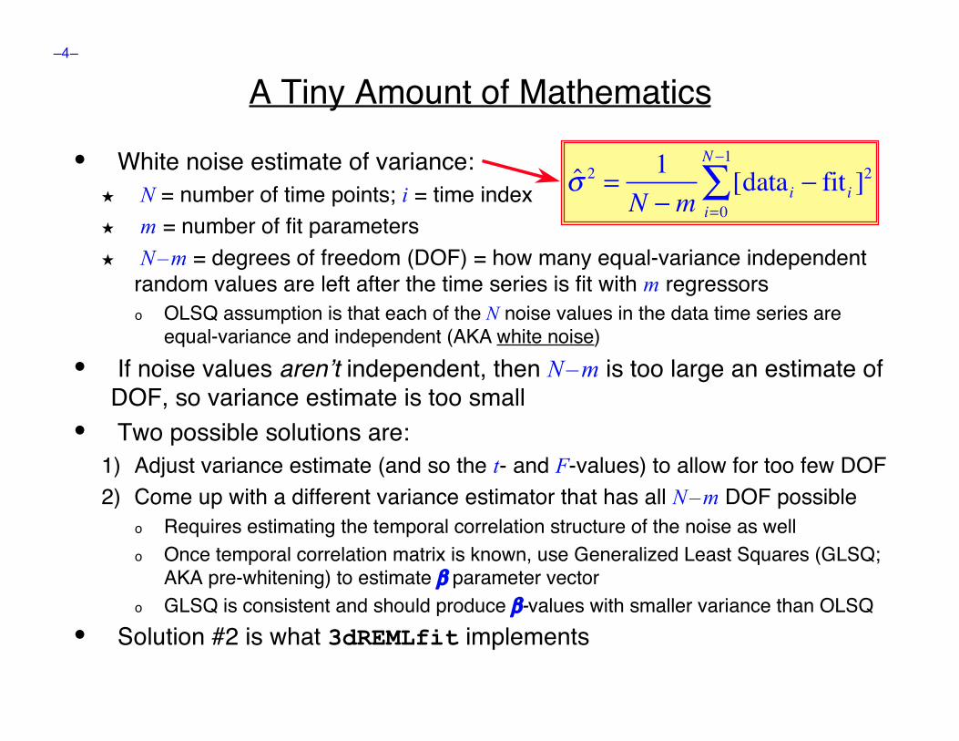
• White noise estimate of variance:★ N = number of time points; i = time index★ m = number of fit parameters★ N – m = degrees of freedom (DOF) = how many equal-variance independent

random values are left after the time series is fit with m regressorso OLSQ assumption is that each of the N noise values in the data time series are

equal-variance and independent (AKA white noise)• If noise values arenʼt independent, then N – m is too large an estimate of

DOF, so variance estimate is too small• Two possible solutions are:

1) Adjust variance estimate (and so the t- and F-values) to allow for too few DOF2) Come up with a different variance estimator that has all N – m DOF possible

o Requires estimating the temporal correlation structure of the noise as wello Once temporal correlation matrix is known, use Generalized Least Squares (GLSQ;

AKA pre-whitening) to estimate β parameter vectoro GLSQ is consistent and should produce β-values with smaller variance than OLSQ

• Solution #2 is what 3dREMLfit implements

!̂2=

1

N " m[data

i" fit

i

i=0

N"1

# ]2

–5–

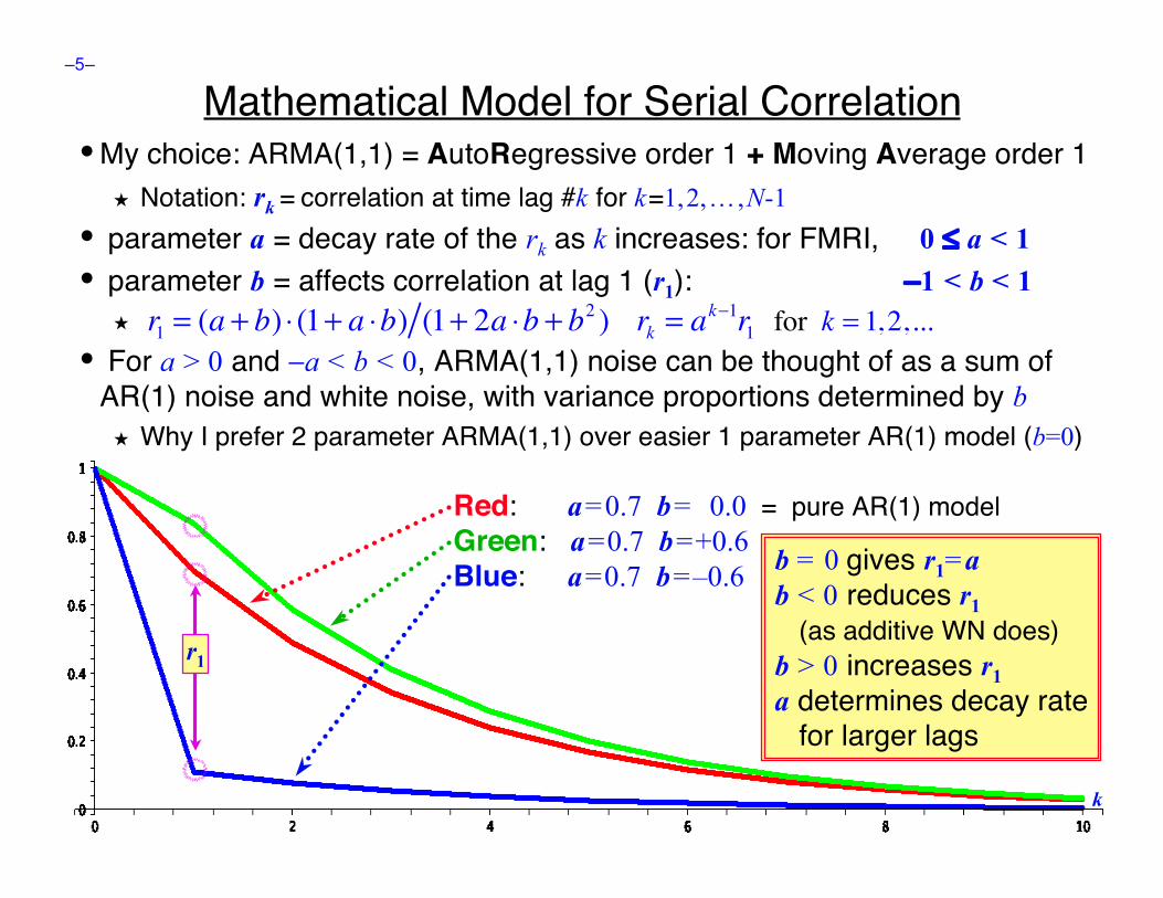
Mathematical Model for Serial Correlation•My choice: ARMA(1,1) = AutoRegressive order 1 + Moving Average order 1

★ Notation: rk = correlation at time lag #k for k =1, 2, … , N-1• parameter a = decay rate of the rk as k increases: for FMRI, 0 ≤ a < 1• parameter b = affects correlation at lag 1 (r1): −1 < b < 1

★

• For a > 0 and −a < b < 0, ARMA(1,1) noise can be thought of as a sum ofAR(1) noise and white noise, with variance proportions determined by b★ Why I prefer 2 parameter ARMA(1,1) over easier 1 parameter AR(1) model (b=0)

r1= (a + b) ! (1+ a !b) (1+ 2a !b + b

2) r

k= a

k"1r1 for k = 1,2,...

Red: a = 0.7 b = 0.0 = pure AR(1) modelGreen: a = 0.7 b = +0.6Blue: a = 0.7 b = –0.6

k

b = 0 gives r1= ab < 0 reduces r1 (as additive WN does)b > 0 increases r1a determines decay rate for larger lags

r1

–6–

New Program: 3dREMLfit• Implements Solution #2: estimate correlation parameters and use GLSQ

★ REML is a (partially nonlinear) method for simultaneously estimating variance +correlation parameters and estimating regression fit parameters (β s)

★ Each voxel gets a separate estimate of its own correlation parameters (a,b)o Estimates of a and b can be spatially smoothed before they are used to compute the β s

o Can also input a and b directly and skip their estimation (the slow part), if desired, anduse those values to compute the β s

o Variance estimate uses pre-whitened residuals to keep DOF=N – m★ Even if correlation decay parameter a was the same for all voxels, relative

amount of white noise (measured by b) mixed in would vary spatiallyo Sample analyses using 1-parameter AR(1) and MA(1) models shown later

• Inputs to 3dREMLfit★ Run 3dDeconvolve first to setup .xmat.1D matrix file, GLTs, etc.

o Donʼt have to let 3dDeconvolve finish analysis: -x1D_stopo 3dDeconvolve also outputs a command line to run 3dREMLfit with the same

3D+time dataset and the matrix file just created★ Then, input matrix file and 3D+time dataset to 3dREMLfit

• Output datasets are structured to be similar to those in 3dDeconvolve★ It should be easy to adapt scripts that use 3dDeconvolve output files (e.g., for

group analysis) to use the new software

–7–

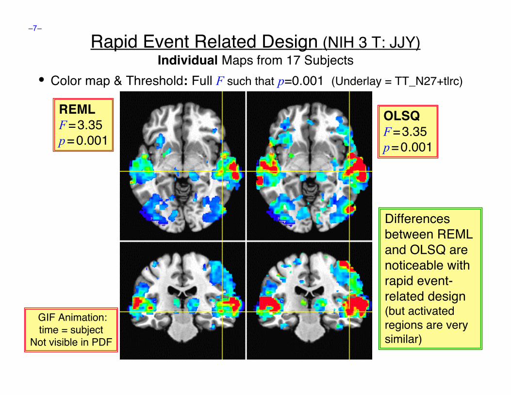
Rapid Event Related Design (NIH 3 T: JJY)Individual Maps from 17 Subjects

• Color map & Threshold: Full F such that p=0.001 (Underlay = TT_N27+tlrc)

REMLF = 3.35p = 0.001

OLSQF = 3.35p = 0.001

GIF Animation:time = subject

Not visible in PDF

Differencesbetween REMLand OLSQ arenoticeable withrapid event-related design(but activatedregions are verysimilar)

–8–

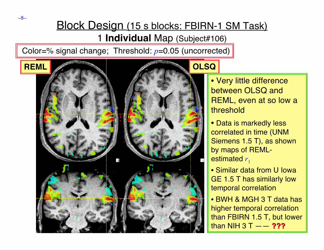
Block Design (15 s blocks: FBIRN-1 SM Task)1 Individual Map (Subject#106)

Color=% signal change; Threshold: p=0.05 (uncorrected)

REML OLSQ• Very little differencebetween OLSQ andREML, even at so low athreshold• Data is markedly lesscorrelated in time (UNMSiemens 1.5 T), as shownby maps of REML-estimated r1

• Similar data from U IowaGE 1.5 T has similarly lowtemporal correlation• BWH & MGH 3 T data hashigher temporal correlationthan FBIRN 1.5 T, but lowerthan NIH 3 T —— ??????

–9–

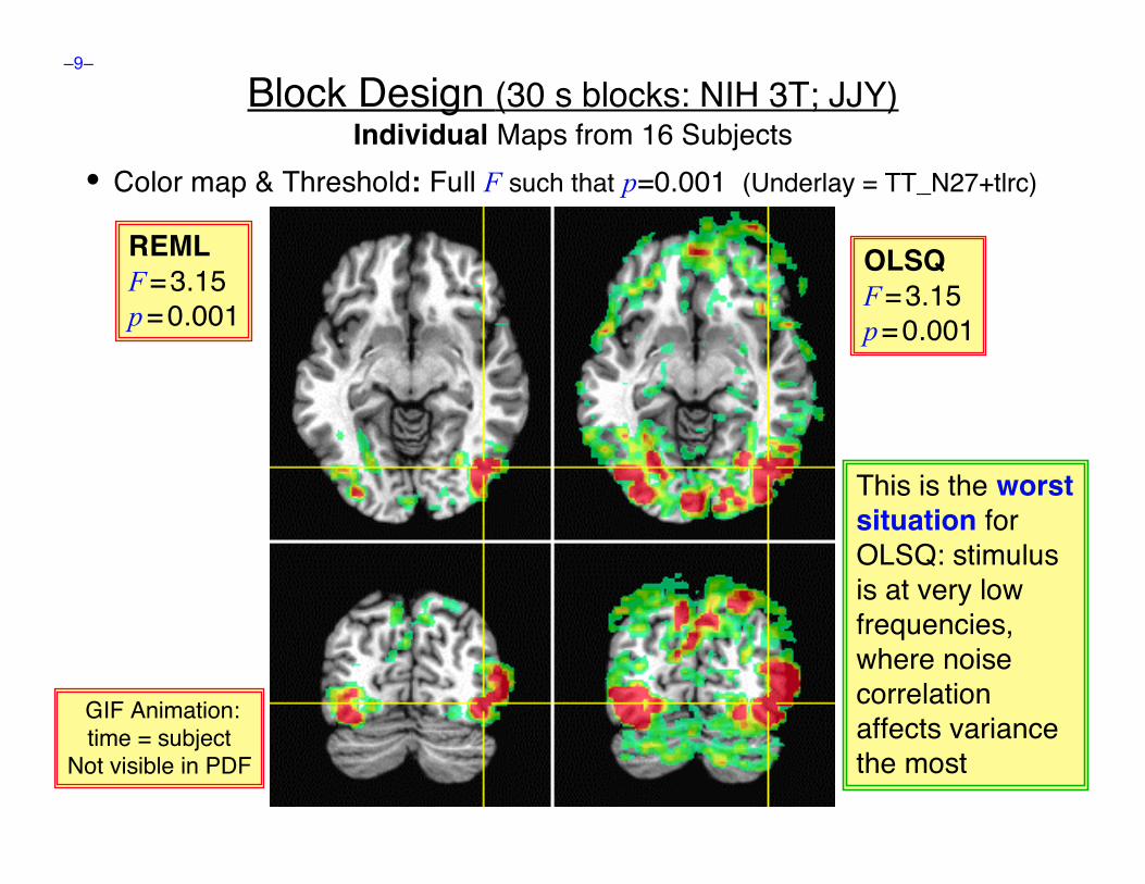
• Color map & Threshold: Full F such that p=0.001 (Underlay = TT_N27+tlrc)

REMLF = 3.15p = 0.001

OLSQF = 3.15p = 0.001

GIF Animation:time = subject

Block Design (30 s blocks: NIH 3T; JJY)Individual Maps from 16 Subjects

This is the worstsituation forOLSQ: stimulusis at very lowfrequencies,where noisecorrelationaffects variancethe most

GIF Animation:time = subject

Not visible in PDF

–10–

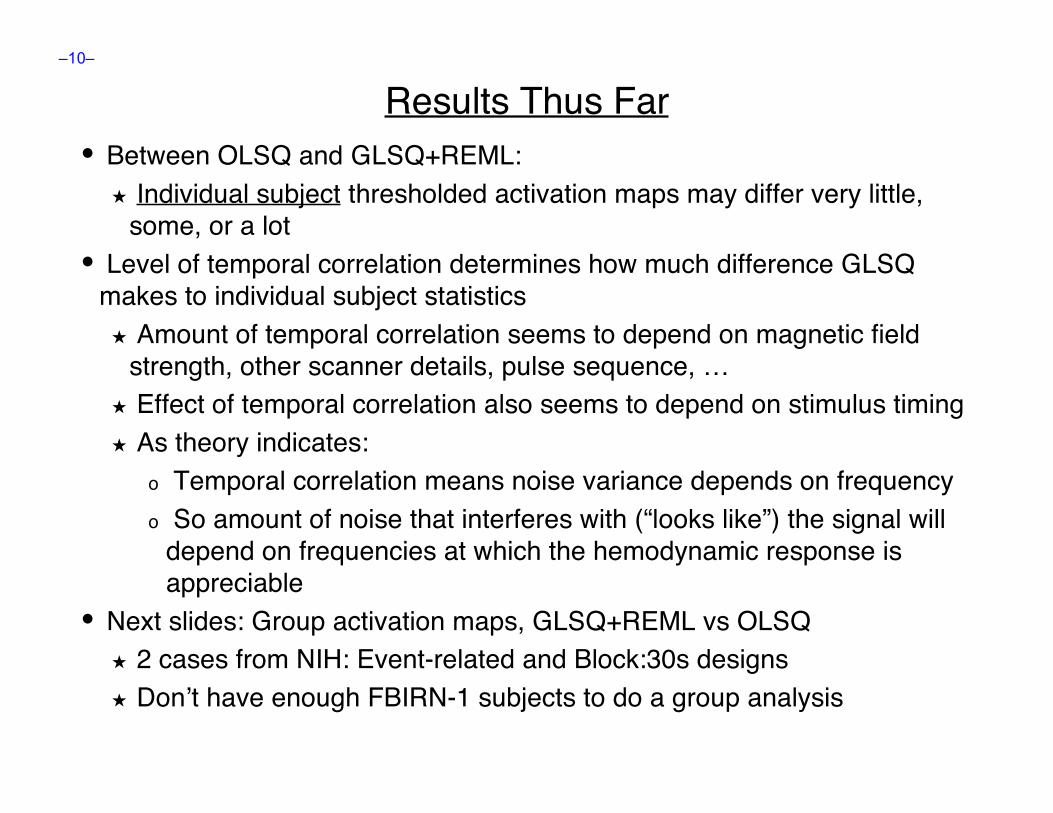
Results Thus Far• Between OLSQ and GLSQ+REML:

★ Individual subject thresholded activation maps may differ very little,some, or a lot

• Level of temporal correlation determines how much difference GLSQmakes to individual subject statistics★ Amount of temporal correlation seems to depend on magnetic field

strength, other scanner details, pulse sequence, …★ Effect of temporal correlation also seems to depend on stimulus timing★ As theory indicates:

o Temporal correlation means noise variance depends on frequencyo So amount of noise that interferes with (“looks like”) the signal will

depend on frequencies at which the hemodynamic response isappreciable

• Next slides: Group activation maps, GLSQ+REML vs OLSQ★ 2 cases from NIH: Event-related and Block:30s designs★ Donʼt have enough FBIRN-1 subjects to do a group analysis

–11–

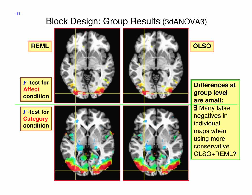
Differences atgroup levelare small:∃ Many falsenegatives inindividualmaps whenusing moreconservativeGLSQ+REML??

Block Design: Group Results (3dANOVA3)

REML OLSQ

F -test forAffectcondition

F -test forCategorycondition

–12–

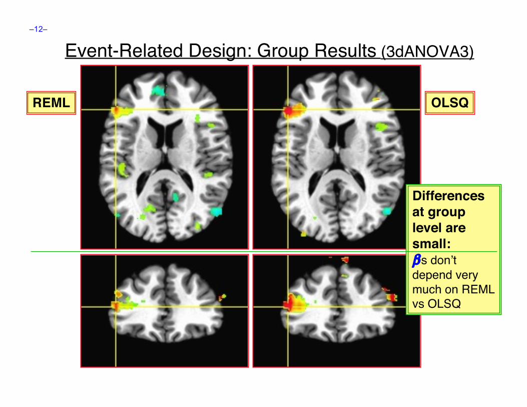
Event-Related Design: Group Results (3dANOVA3)

REML OLSQ

Differencesat grouplevel aresmall:β s donʼtdepend verymuch on REMLvs OLSQ

–13–

Tentative Conclusions• For individual subject thresholded activation maps:

★ Use GLSQ/REML estimation, especially for slow block designexperiments at 3+ Tesla

★ Be aware that there may be many false negativeso i.e., false acceptances of the null hypothesiso am looking into an FDR-like procedure for estimating the false negative rate,

similar to how FDR estimates the false positive rate

• For group maps using ANOVA (or similar statistics):★ Differences between OLSQ and GLSQ estimation are small

• Recommendations:★ Donʼt need to re-visit group activation conclusions!★ Use 3dREMLfit as a near drop-in replacment for 3dDeconvolve for

future work

o A little extra CPU time (usually from 1..3 times as long)

–14–

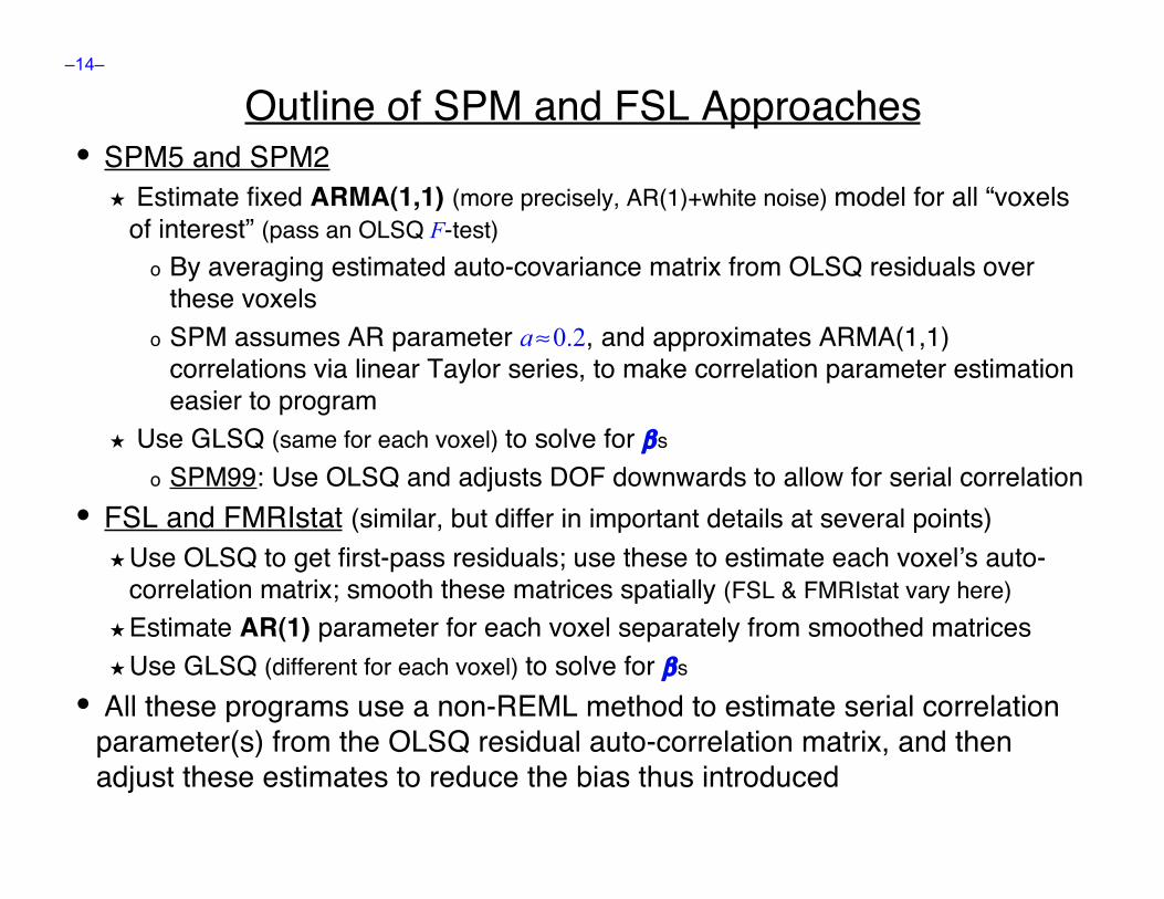
Outline of SPM and FSL Approaches• SPM5 and SPM2

★ Estimate fixed ARMA(1,1) (more precisely, AR(1)+white noise) model for all “voxelsof interest” (pass an OLSQ F-test)

o By averaging estimated auto-covariance matrix from OLSQ residuals overthese voxels

o SPM assumes AR parameter a ≈ 0.2, and approximates ARMA(1,1)correlations via linear Taylor series, to make correlation parameter estimationeasier to program

★ Use GLSQ (same for each voxel) to solve for β s

o SPM99: Use OLSQ and adjusts DOF downwards to allow for serial correlation• FSL and FMRIstat (similar, but differ in important details at several points)

★Use OLSQ to get first-pass residuals; use these to estimate each voxelʼs auto-correlation matrix; smooth these matrices spatially (FSL & FMRIstat vary here)

★Estimate AR(1) parameter for each voxel separately from smoothed matrices★Use GLSQ (different for each voxel) to solve for β s

• All these programs use a non-REML method to estimate serial correlationparameter(s) from the OLSQ residual auto-correlation matrix, and thenadjust these estimates to reduce the bias thus introduced

–15–

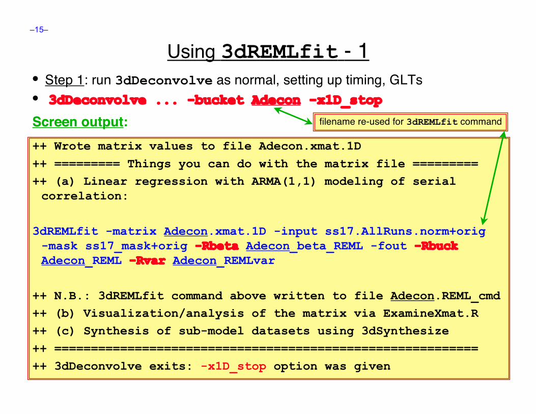
Using 3dREMLfit - 1• Step 1: run 3dDeconvolve as normal, setting up timing, GLTs• 3dDeconvolve ... -bucket Adecon -x1D_stopScreen outputScreen output:++ Wrote matrix values to file Adecon.xmat.1D++ ========= Things you can do with the matrix file =========++ (a) Linear regression with ARMA(1,1) modeling of serialcorrelation:

3dREMLfit -matrix Adecon.xmat.1D -input ss17.AllRuns.norm+orig-mask ss17_mask+orig -Rbeta Adecon_beta_REML -fout -RbuckAdecon_REML -Rvar Adecon_REMLvar

++ N.B.: 3dREMLfit command above written to file Adecon.REML_cmd++ (b) Visualization/analysis of the matrix via ExamineXmat.R++ (c) Synthesis of sub-model datasets using 3dSynthesize++ ==========================================================++ 3dDeconvolve exits: -x1D_stop option was given

filename re-used for 3dREMLfit command

–16–

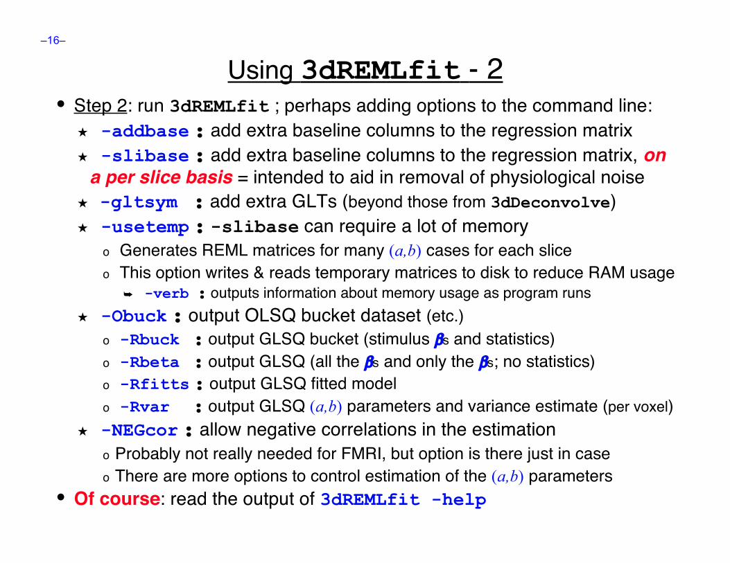
Using 3dREMLfit - 2• Step 2: run 3dREMLfit ; perhaps adding options to the command line:

★ -addbase : add extra baseline columns to the regression matrix★ -slibase : add extra baseline columns to the regression matrix, on

a per slice basis = intended to aid in removal of physiological noise★ -gltsym : add extra GLTs (beyond those from 3dDeconvolve)★ -usetemp : -slibase can require a lot of memory

o Generates REML matrices for many (a,b) cases for each sliceo This option writes & reads temporary matrices to disk to reduce RAM usage

➥ -verb : outputs information about memory usage as program runs★ -Obuck : output OLSQ bucket dataset (etc.)

o -Rbuck : output GLSQ bucket (stimulus βs and statistics)o -Rbeta : output GLSQ (all the βs and only the βs; no statistics)o -Rfitts : output GLSQ fitted modelo -Rvar : output GLSQ (a,b) parameters and variance estimate (per voxel)

★ -NEGcor : allow negative correlations in the estimationo Probably not really needed for FMRI, but option is there just in caseo There are more options to control estimation of the (a,b) parameters

• Of course: read the output of 3dREMLfit -help

–17–

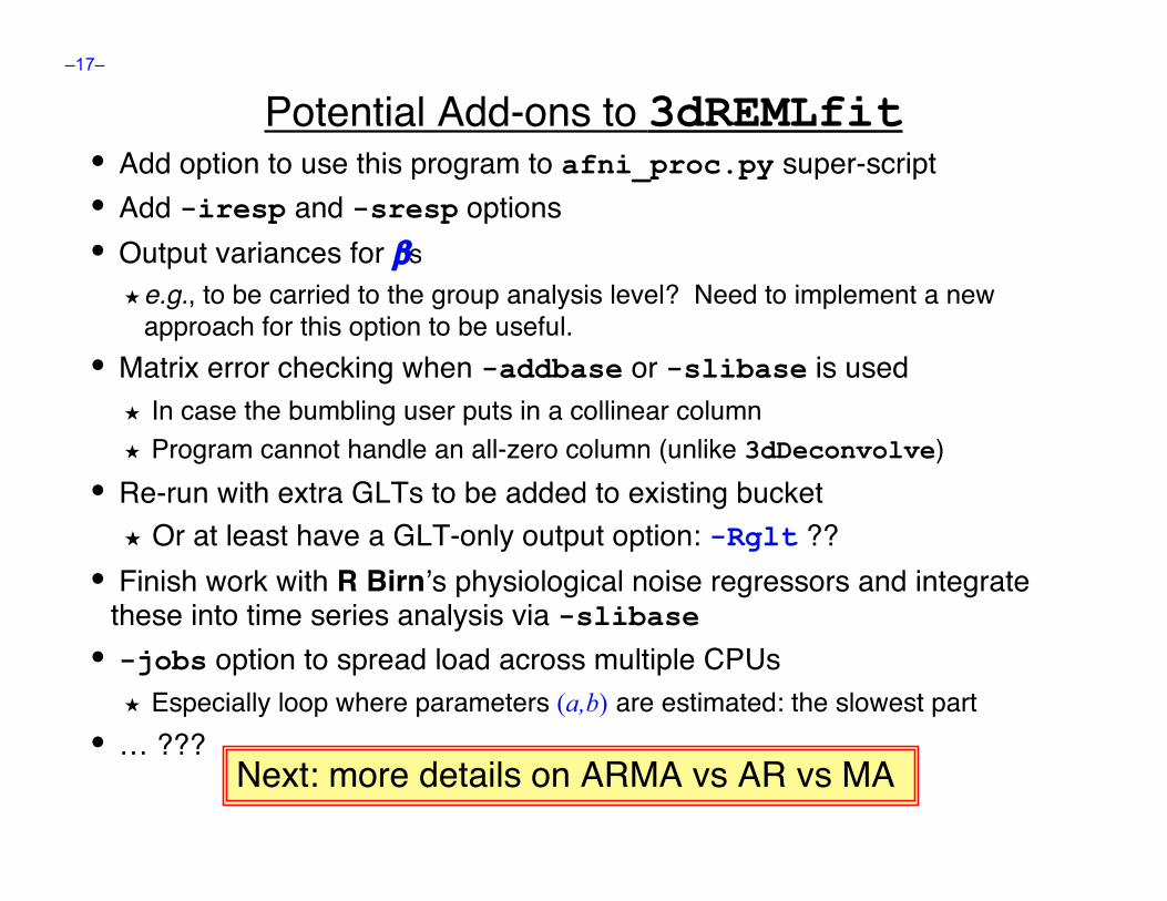
Potential Add-ons to 3dREMLfit• Add option to use this program to afni_proc.py super-script• Add -iresp and -sresp options• Output variances for βs

★e.g., to be carried to the group analysis level? Need to implement a newapproach for this option to be useful.

• Matrix error checking when -addbase or -slibase is used★ In case the bumbling user puts in a collinear column★ Program cannot handle an all-zero column (unlike 3dDeconvolve)

• Re-run with extra GLTs to be added to existing bucket★ Or at least have a GLT-only output option: -Rglt ??

• Finish work with R Birnʼs physiological noise regressors and integratethese into time series analysis via -slibase• -jobs option to spread load across multiple CPUs

★ Especially loop where parameters (a,b) are estimated: the slowest part• … ???

Next: more details on ARMA vs AR vs MA

–18–

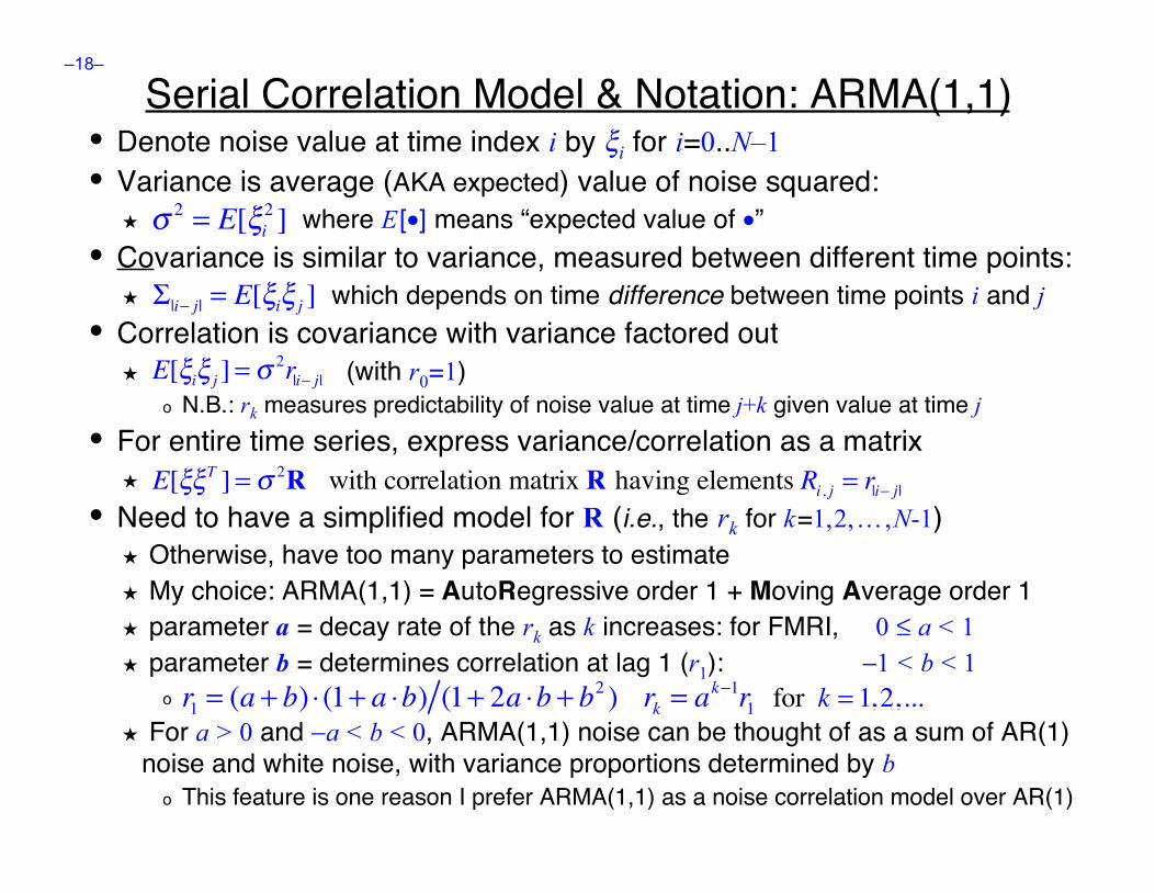
Serial Correlation Model & Notation: ARMA(1,1)• Denote noise value at time index i by ξi for i=0..N–1• Variance is average (AKA expected) value of noise squared:

★ where E [•] means “expected value of •”• Covariance is similar to variance, measured between different time points:

★ which depends on time difference between time points i and j• Correlation is covariance with variance factored out

★ (with r0=1)o N.B.: rk measures predictability of noise value at time j+k given value at time j

• For entire time series, express variance/correlation as a matrix★

• Need to have a simplified model for R (i.e., the rk for k =1, 2, … , N-1)★ Otherwise, have too many parameters to estimate★ My choice: ARMA(1,1) = AutoRegressive order 1 + Moving Average order 1★ parameter a = decay rate of the rk as k increases: for FMRI, 0 ≤ a < 1★ parameter b = determines correlation at lag 1 (r1): −1 < b < 1

o

★ For a > 0 and −a < b < 0, ARMA(1,1) noise can be thought of as a sum of AR(1)noise and white noise, with variance proportions determined by b

o This feature is one reason I prefer ARMA(1,1) as a noise correlation model over AR(1)

! 2= E["

i

2]

!|i" j| = E[#i# j

]

E[!i!j] = " 2

r|i# j|

E[!!T ] = " 2R with correlation matrix R having elements R

i, j = r|i# j|

r1= (a + b) ! (1+ a !b) (1+ 2a !b + b

2) r

k= a

k"1r1 for k = 1,2,...

–19–

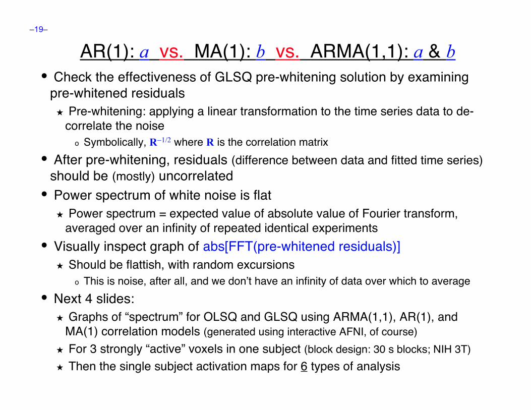
AR(1): a vs. MA(1): b vs. ARMA(1,1): a & b• Check the effectiveness of GLSQ pre-whitening solution by examining

pre-whitened residuals★ Pre-whitening: applying a linear transformation to the time series data to de-

correlate the noiseo Symbolically, R−1/2 where R is the correlation matrix

• After pre-whitening, residuals (difference between data and fitted time series)should be (mostly) uncorrelated• Power spectrum of white noise is flat

★ Power spectrum = expected value of absolute value of Fourier transform,averaged over an infinity of repeated identical experiments

• Visually inspect graph of abs[FFT(pre-whitened residuals)]★ Should be flattish, with random excursions

o This is noise, after all, and we donʼt have an infinity of data over which to average• Next 4 slides:

★ Graphs of “spectrum” for OLSQ and GLSQ using ARMA(1,1), AR(1), andMA(1) correlation models (generated using interactive AFNI, of course)

★ For 3 strongly “active” voxels in one subject (block design: 30 s blocks; NIH 3T)★ Then the single subject activation maps for 6 types of analysis

–20–

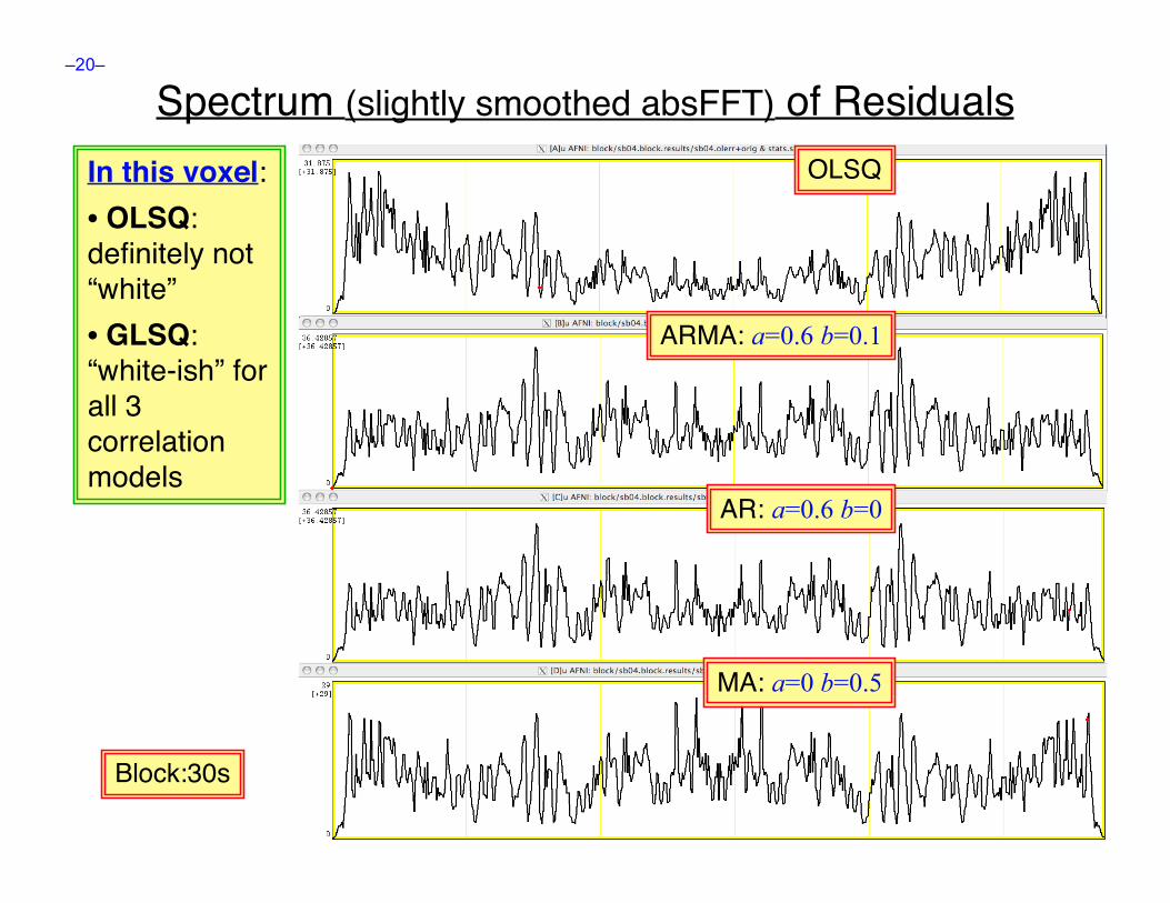
Spectrum (slightly smoothed absFFT) of ResidualsOLSQ

ARMA: a=0.6 b=0.1

AR: a=0.6 b=0

MA: a=0 b=0.5

In this voxel:• OLSQ:definitely not“white”• GLSQ:“white-ish” forall 3correlationmodels

Block:30s

–21–

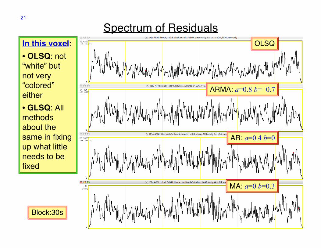
Spectrum of ResidualsOLSQIn this voxel:

• OLSQ: not“white” butnot very“colored”either• GLSQ: Allmethodsabout thesame in fixingup what littleneeds to befixed

Block:30s

ARMA: a=0.8 b= –0.7

AR: a=0.4 b=0

MA: a=0 b=0.3

–22–

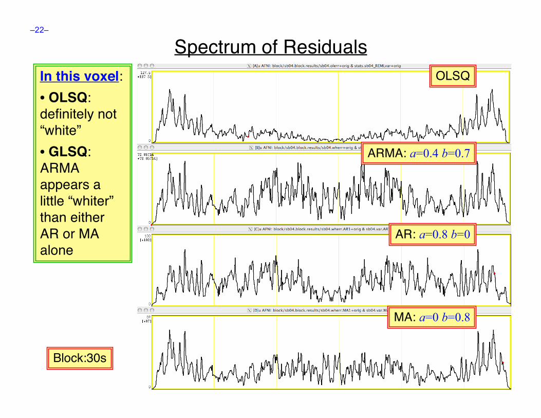
Spectrum of ResidualsOLSQIn this voxel:

• OLSQ:definitely not“white”• GLSQ:ARMAappears alittle “whiter”than eitherAR or MAalone

Block:30s

ARMA: a=0.4 b=0.7

AR: a=0.8 b=0

MA: a=0 b=0.8

–23–

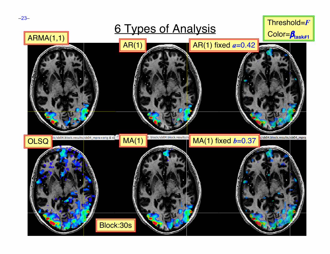
6 Types of Analysis

OLSQ MA(1)

AR(1)ARMA(1,1)

Threshold=FColor=βtask#1

MA(1) fixed b=0.37

AR(1) fixed a=0.42

Block:30s

–24–

Conclusions from Previous Slides• It is possible to find voxels where pre-whitening of different types (AR-

only or MA-only or ARMA) is “optimal”★ And voxels where pre-whitening makes little difference

• For many (most?) voxels, the pre-whitening details donʼt make a lot ofdifference in the statistics★ As long as something is done that is about right★ e.g., Using fixed AR(1) or MA(1) single parameter method was still OK-ish for

single subject mapso A few more extraneous small blobso But fewer than pure OLSQ solution statistics

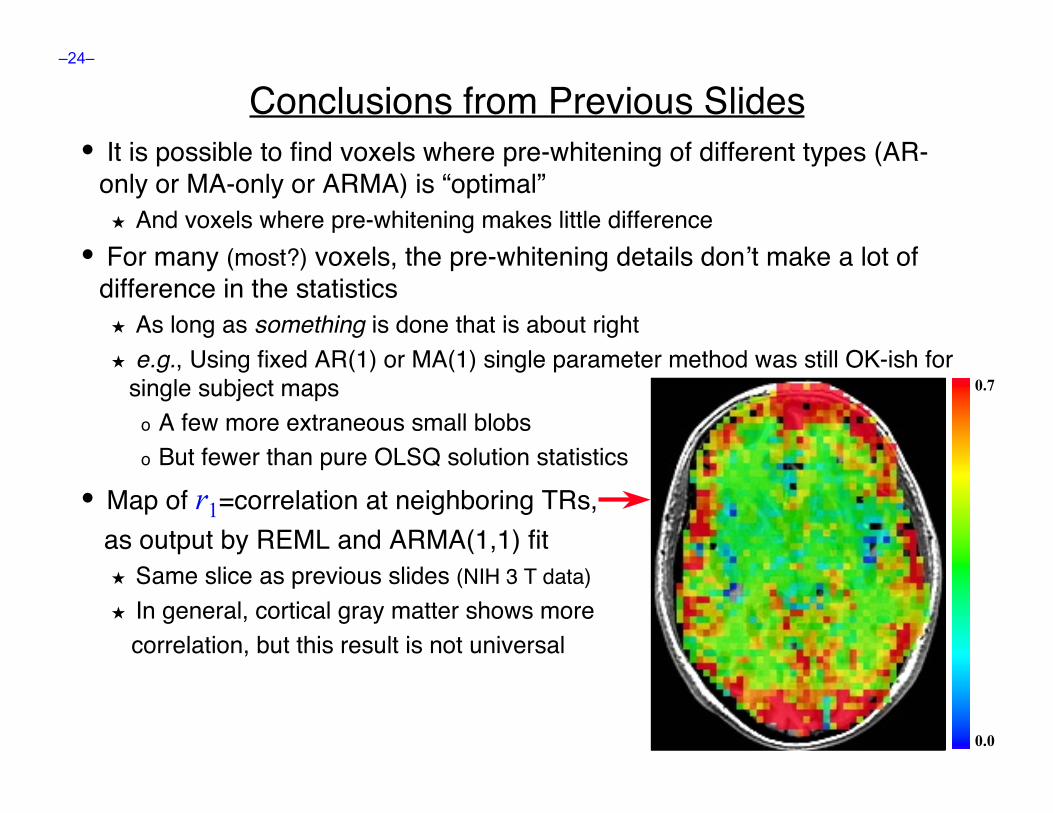
• Map of r1=correlation at neighboring TRs, as output by REML and ARMA(1,1) fit

★ Same slice as previous slides (NIH 3 T data)★ In general, cortical gray matter shows more correlation, but this result is not universal

0.0

0.7

–25–

Mathematics and Implementation• Available in PDF (scanned from hand-written pages) for the truly devoted

★ File 3dREMLfit_mathnotes.pdf• Outline of REML estimation methodology

★ What is REML and why do we care?• Matrix algebra for efficient solution of the many linear systems that must

be solved for each voxel★ Sparse matrix factorizations, multiplications, and solvers

• How ARMA(1,1) parameters are estimated in 3dREMLfit★ Optimizing REML log-likelihood function over a discrete grid of (a,b)

values, using 2D binary search★ Must solve a GLSQ problem for each (a,b) tested, for each voxel

• How statistics are implemented as GLTs★ Testing null hypothesis Gβ=0 for arbitrary matrix G

• Derivation of ARMA(1,1) formulas★ For completeness, and because we all love equations