AdaptivelyBiased

MolecularDynamics

Volodymyr Babin, Christopher Roland and Celeste Sagui

Department of Physics, NC State University,Raleigh, NC 27695-8202

1

The Talk Outline:

• Problem statement

• Metadynamics (+ Applications)

• ABMD (+ Applications)

2

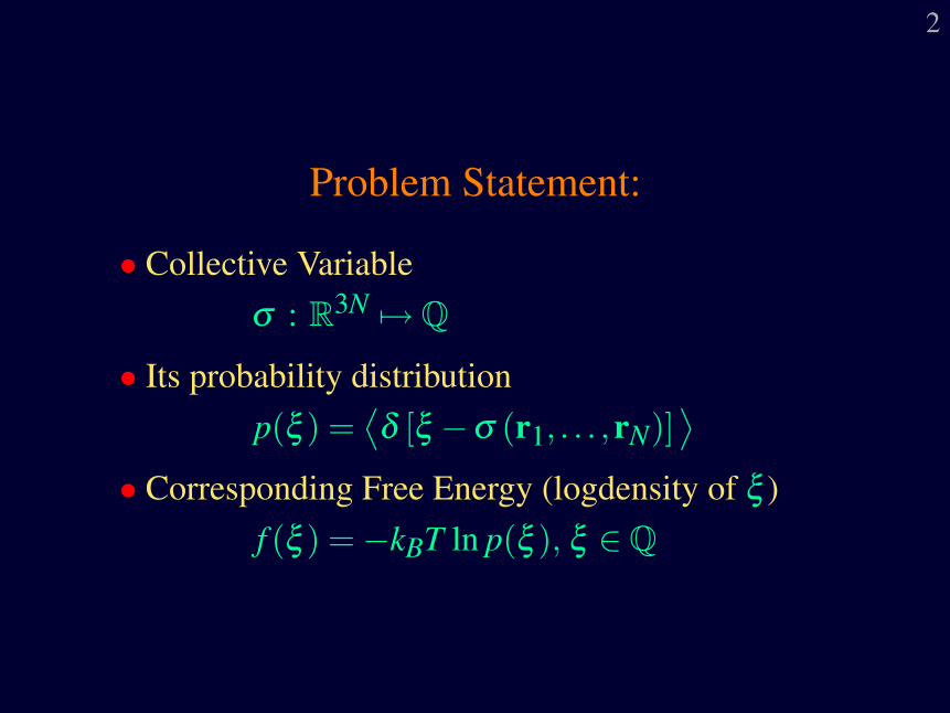
Problem Statement:

• Collective Variableσ : R3N 7→Q

• Its probability distributionp(ξ ) =

⟨δ [ξ −σ (r1, . . . ,rN)]

⟩• Corresponding Free Energy (logdensity of ξ )

f (ξ ) =−kBT ln p(ξ ), ξ ∈Q

3

The Free Energy f (ξ ):

• Describes the relative stability ofdifferent states.

• Provides useful insights into thetransitions between these states.

4

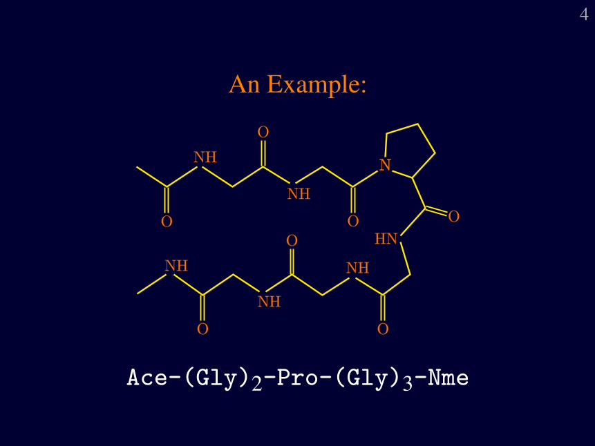
An Example:

Ace-(Gly)2-Pro-(Gly)3-Nme

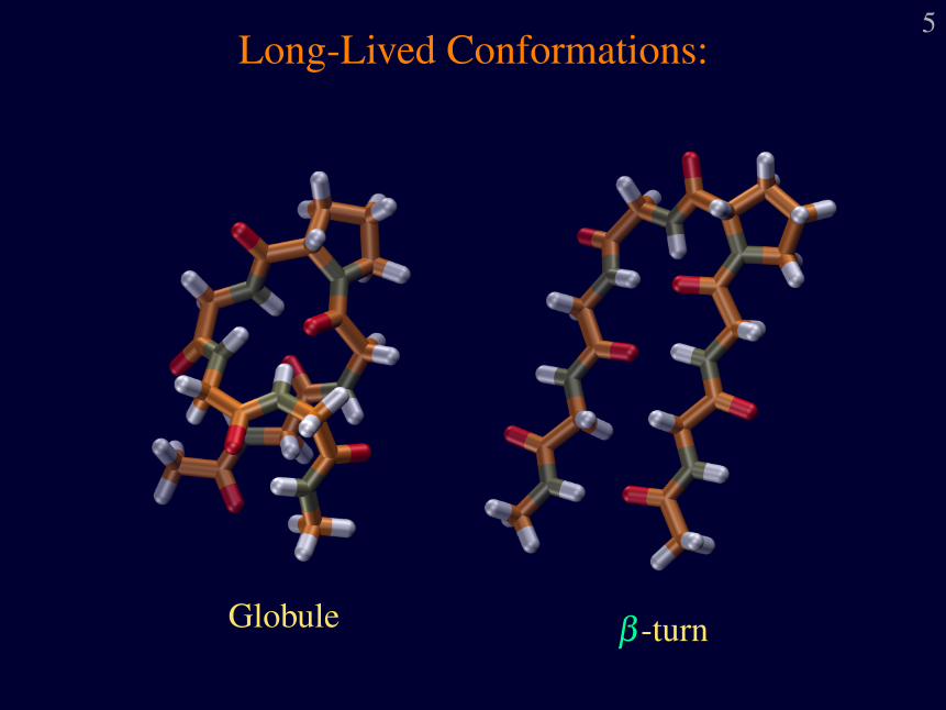
5Long-Lived Conformations:

Globuleβ -turn

6

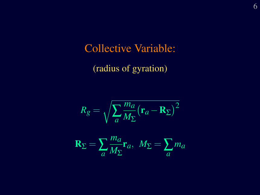
Collective Variable:

(radius of gyration)

Rg =√

∑a

maMΣ

(ra−RΣ

)2RΣ = ∑

a

maMΣ

ra, MΣ = ∑a

ma

7

Why the Rg ?

• It provides a sensible description of theconformations in terms of just one number.

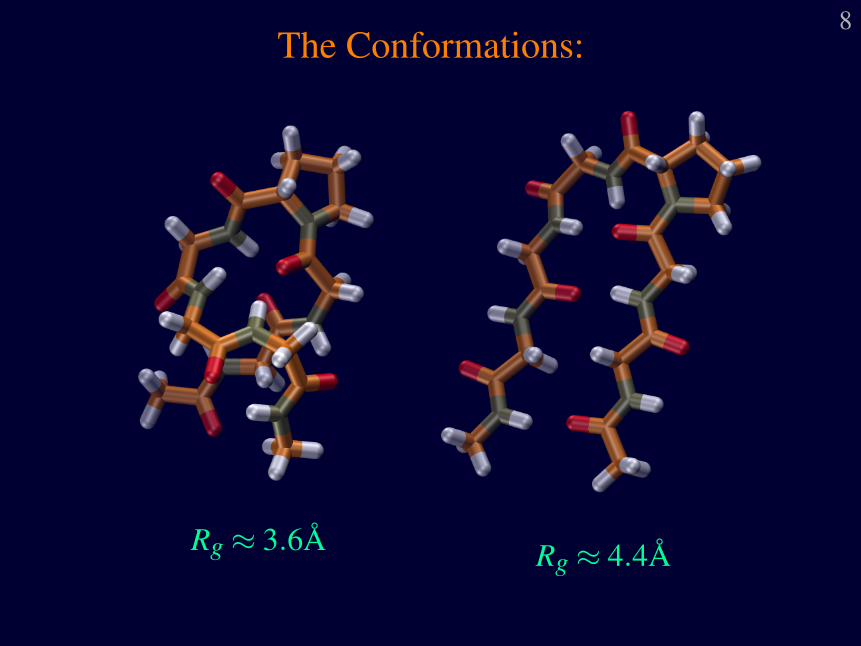
8The Conformations:

Rg ≈ 3.6A Rg ≈ 4.4A

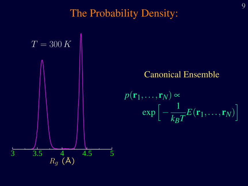
9The Probability Density:

3 3.5 4 4.5 5Rg (A)

T = 300 K

Canonical Ensemble

p(r1, . . . ,rN) ∝

exp[− 1

kBTE(r1, . . . ,rN)

]

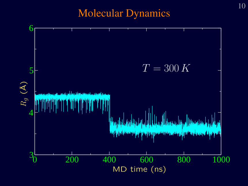
10Molecular Dynamics

0 200 400 600 800 10003

4

5

6

MD time (ns)

Rg

(A)

T = 300 K

11

The Problems:

• MD trajectory rarely jumps through the barriers (i.e.,the MD is bad for sampling from the canonical dis-tribution; this can be “cured” by using, e.g., paralleltempering).

• MD trajectory is trapped near the free energy minima(canonical ensemble).

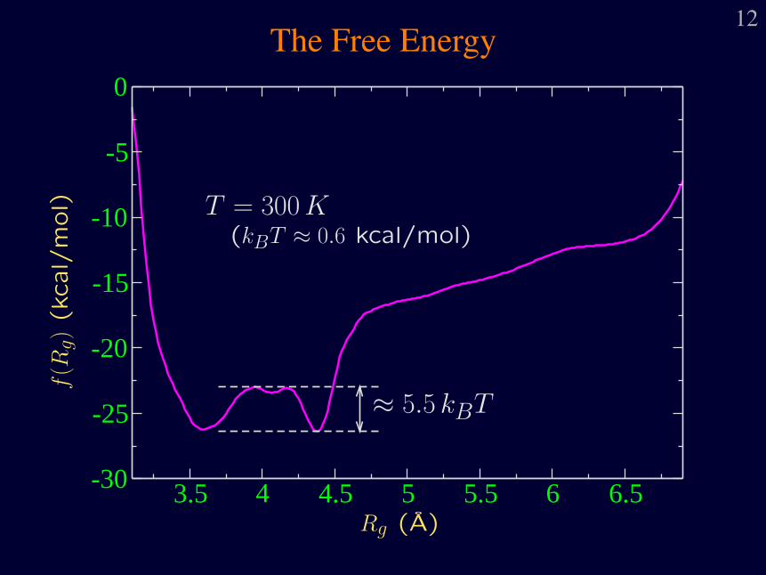
12The Free Energy

3.5 4 4.5 5 5.5 6 6.5-30

-25

-20

-15

-10

-5

0

Rg (A)

f(R

g)(k

cal/

mol) T = 300 K

(kBT ≈ 0.6 kcal/mol)

≈ 5.5 kBT

13

“Classical” Remedies:

• Better ways of sampling from the canonicaldistribution (replica exchange).

• Sampling from a biased distribution with thebias that can be “undone” afterwards (umbrellasampling).

14Non-Equilibrium Methods

• Local Elevation (MD context)

T. HUBER, A. E. TORDA, AND W. F. VAN GUNSTEREN, Local elevation:a method for improving the searching properties of molecular dynamicssimulation, J. Comput. Aided. Mol. Des., 8 (1994), pp. 695–708.

• Wang-Landau (MC context)

F. WANG AND D. P. LANDAU, Efficient, multiple-range random walkalgorithm to calculate the density of states, Phys. Rev. Lett., 86 (2001),pp. 2050–2053.

15Non-Equilibrium Methods

• Adaptive Force Bias

E. DARVE AND A. POHORILLE, Calculating free energies using averageforce, J. Chem. Phys., 115 (2001), pp. 9169–9183.

J. HENIN AND C. CHIPOT, Overcoming free energy barriers using uncon-strained molecular dynamics simulations., J. Chem. Phys., 121 (2004),pp. 2904–2914.

• Metadynamics

M. IANNUZZI, A. LAIO, AND M. PARRINELLO, Efficient exploration ofreactive potential energy surfaces using Car-Parrinello molecular dynam-ics, Phys. Rev. Lett., 90 (2003), pp. 238302–1.

16

Ingredients of a Non-Equilibrium Method:

• Sampling Device (typically MolecularDynamics or Replica-Exchange Molec-ular Dynamics).

and

• Non-stationary Biasing potential.

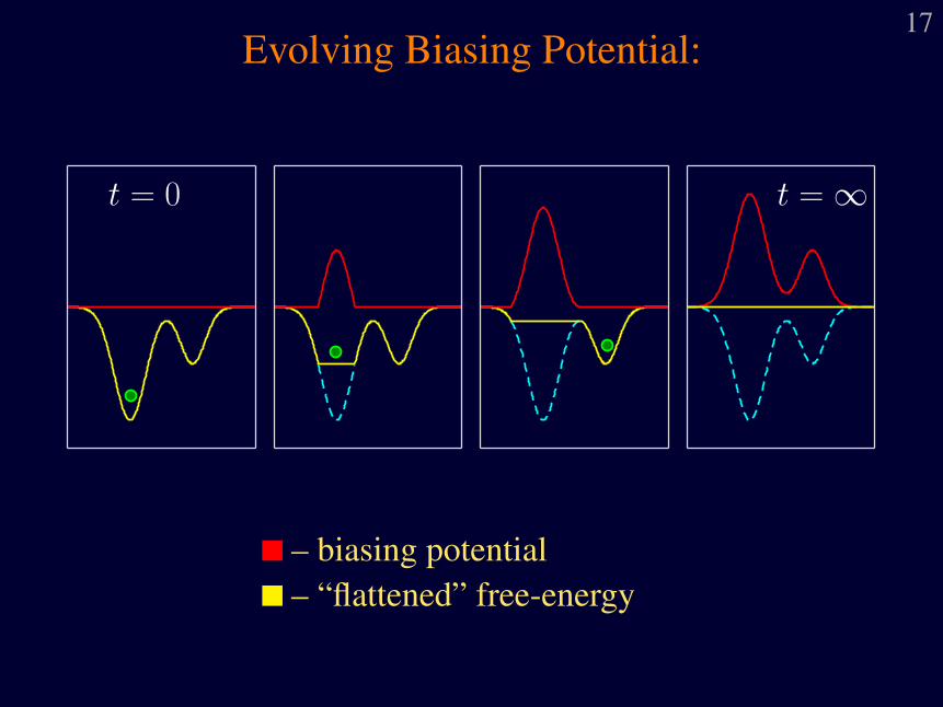
17Evolving Biasing Potential:

t = 0 t =∞

– biasing potential– “flattened” free-energy

18

Metadynamics References

A. LAIO AND M. PARRINELLO, Escaping free-energy minima, Proc.Natl. Acad. Sci., 99 (2002), pp. 12562– 12566.

M. IANNUZZI, A. LAIO, AND M. PARRINELLO, Efficient exploration ofreactive potential energy surfaces using Car-Parrinello molecular dynam-ics, Phys. Rev. Lett., 90 (2003), pp. 238302–1.

19

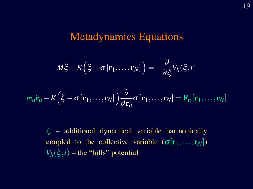
Metadynamics Equations

Mξ +K(

ξ −σ [r1, . . . ,rN])

=− ∂

∂ξVh(ξ , t)

mara−K(

ξ −σ [r1, . . . ,rN])

∂

∂raσ [r1, . . . ,rN] = Fa [r1, . . . ,rN]

ξ – additional dynamical variable harmonicallycoupled to the collective variable (σ [r1, . . . ,rN])Vh(ξ , t) – the “hills” potential

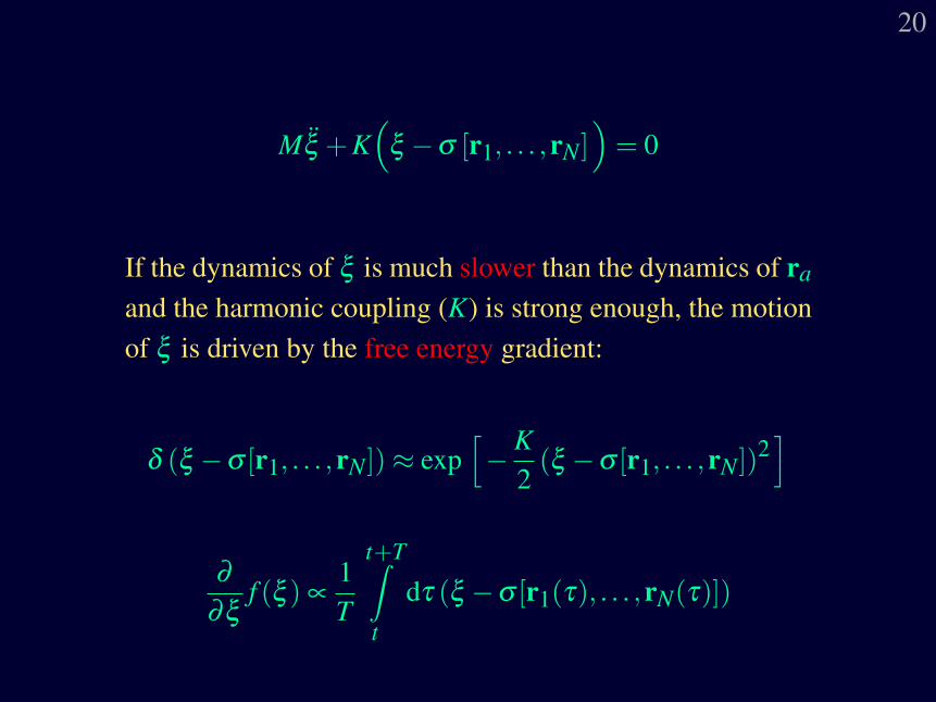
20

Mξ +K(

ξ −σ [r1, . . . ,rN])

= 0

If the dynamics of ξ is much slower than the dynamics of ra

and the harmonic coupling (K) is strong enough, the motionof ξ is driven by the free energy gradient:

δ (ξ −σ [r1, . . . ,rN])≈ exp[−K

2(ξ −σ [r1, . . . ,rN])2

]

∂

∂ξf (ξ ) ∝

1T

t+T∫t

dτ (ξ −σ [r1(τ), . . . ,rN(τ)])

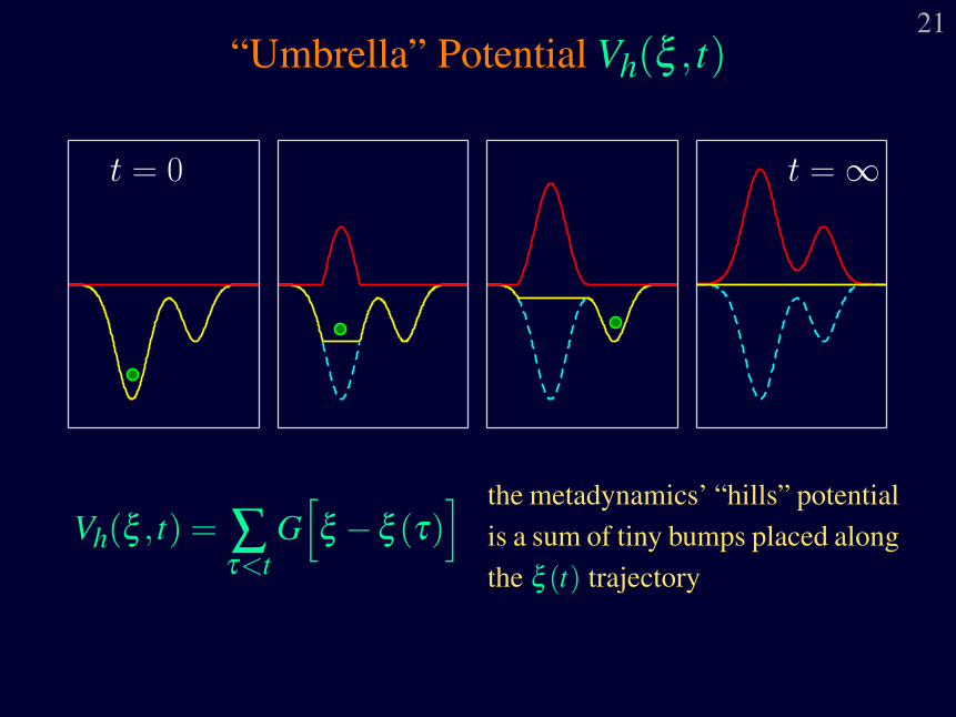
21“Umbrella” Potential Vh(ξ , t)

t = 0 t =∞

Vh(ξ , t) = ∑τ<t

G[ξ −ξ (τ)

] the metadynamics’ “hills” potentialis a sum of tiny bumps placed alongthe ξ (t) trajectory

22

As-Is Metadynamics is O(t2):

• The number of terms (bumps) in Vh(ξ , t) (the“hills” potential) at time t is proportional to t.

• Vh(ξ , t) must be computed at every MD step.

23

Metadynamics / Applications

E. ASCIUTTO AND C. SAGUI, Exploring Intramolecular Reactions inComplex Systems with Metadynamics: The Case of the Malonate An-ions, J. Phys. Chem. A, 109 (2005), pp. 7682–7687.

J. G. LEE, E. ASCIUTTO, V. BABIN, C. SAGUI, T. A. DARDEN ANDC. ROLAND, Deprotonation of Solvated Formic Acid: Car-Parrinello andMetadynamics Simulations, J. Phys. Chem. B, 110 (2006) pp. 2325–2331.

24

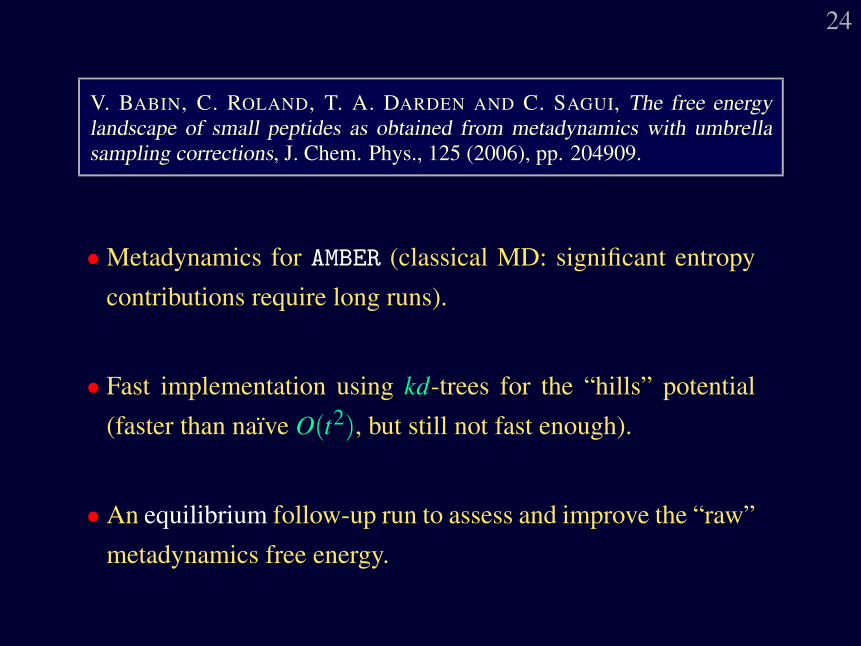
V. BABIN, C. ROLAND, T. A. DARDEN AND C. SAGUI, The free energylandscape of small peptides as obtained from metadynamics with umbrellasampling corrections, J. Chem. Phys., 125 (2006), pp. 204909.

• Metadynamics for AMBER (classical MD: significant entropy

contributions require long runs).

• Fast implementation using kd-trees for the “hills” potential

(faster than naıve O(t2), but still not fast enough).

• An equilibrium follow-up run to assess and improve the “raw”

metadynamics free energy.

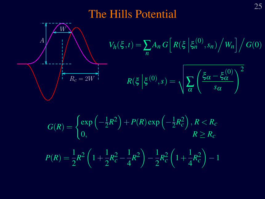
25The Hills Potential

W

A

Rc = 2W

Vh(ξ , t) = ∑n

An G[

R(ξ∣∣∣ξ (0)

n ,sn)/

Wn

]/G(0)

R(ξ∣∣∣ξ (0),s) =

√√√√∑α

(ξα−ξ

(0)α

sα

)2

G(R) =

{exp(−1

2R2)

+P(R)exp(−1

2R2c

), R < Rc

0, R≥ Rc

P(R) =12

R2(

1+12

R2c−

14

R2)− 1

2R2

c

(1+

14

R2c

)−1

26

How to check the accuracy ?

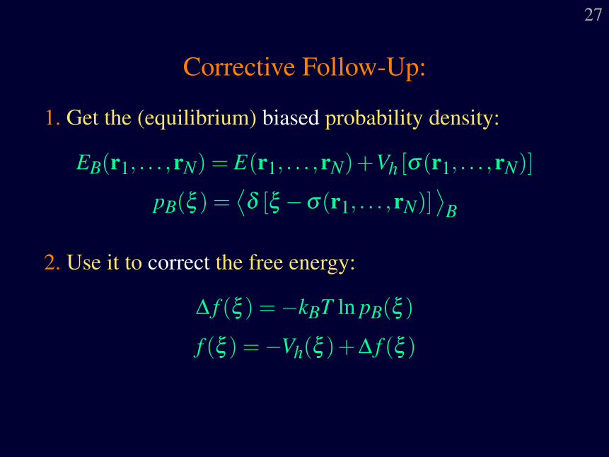
27

Corrective Follow-Up:

1. Get the (equilibrium) biased probability density:

EB(r1, . . . ,rN) = E(r1, . . . ,rN)+Vh [σ(r1, . . . ,rN)]

pB(ξ ) =⟨δ [ξ −σ(r1, . . . ,rN)]

⟩B

2. Use it to correct the free energy:

∆ f (ξ ) =−kBT ln pB(ξ )

f (ξ ) =−Vh(ξ )+∆ f (ξ )

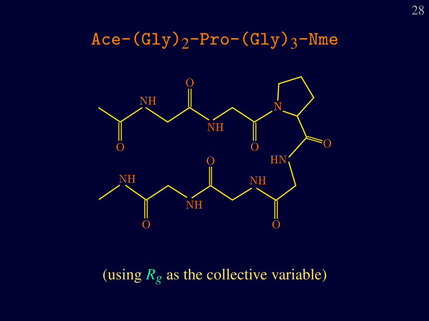
28

Ace-(Gly)2-Pro-(Gly)3-Nme

(using Rg as the collective variable)

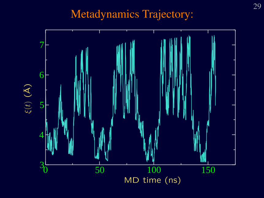
29Metadynamics Trajectory:

0 50 100 1503

4

5

6

7

MD time (ns)

ξ(t

)(A)

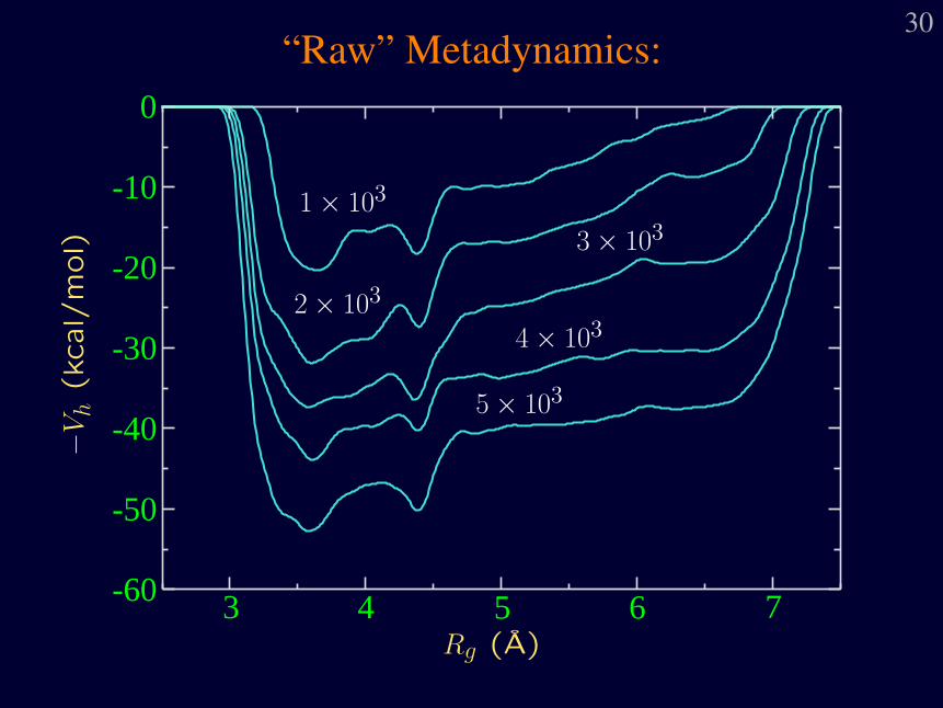
30“Raw” Metadynamics:

3 4 5 6 7-60

-50

-40

-30

-20

-10

0

Rg (A)

−V

h(k

cal/

mol)

1 × 103

2 × 103

3 × 103

4 × 103

5 × 103

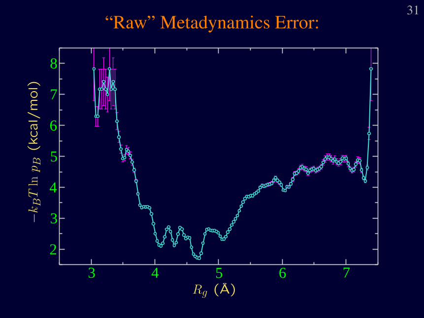
31“Raw” Metadynamics Error:

3 4 5 6 7

2

3

4

5

6

7

8

Rg (A)

−kB

Tln

pB

(kcal/

mol)

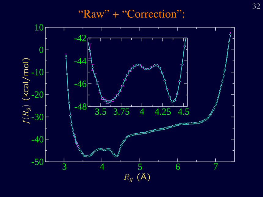
32“Raw” + “Correction”:

3 4 5 6 7-50

-40

-30

-20

-10

0

10

3.5 3.75 4 4.25 4.5-48

-46

-44

-42

Rg (A)

f(R

g)(k

cal/

mol)

33

The “raw” error of ≈ 5kBT is unacceptable(it is comparable with the barrier height)!The equilibrium follow-up is therefore cru-cial to get accurate results.

34

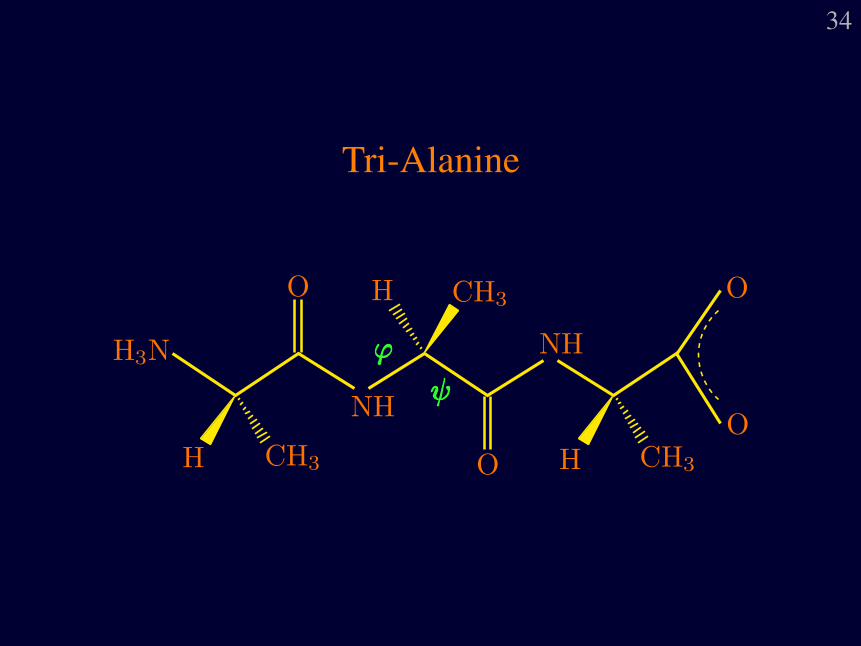
Tri-Alanine

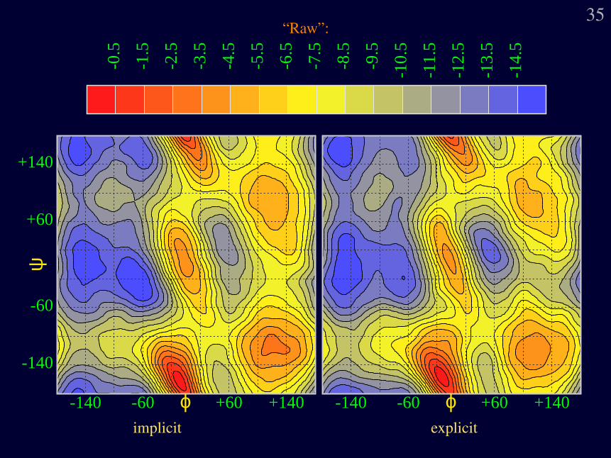
35“Raw”:

-14.

5

-13.

5

-12.

5

-11.

5

-10.

5

-9.5

-8.5

-7.5

-6.5

-5.5

-4.5

-3.5

-2.5

-1.5

-0.5

-140 -60 +60 +140

-140

-60

+60

+140

ϕ

ψ

-140 -60 +60 +140ϕimplicit explicit

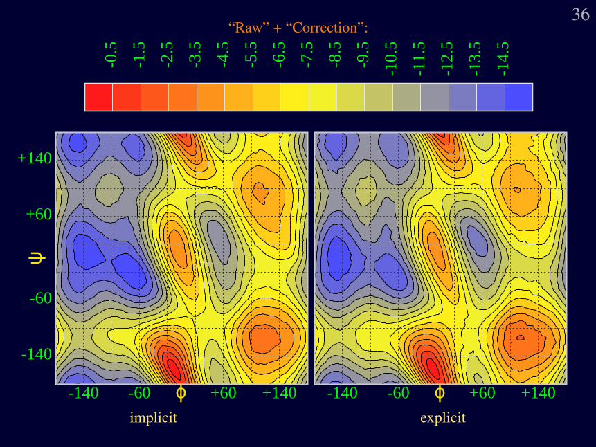
36“Raw” + “Correction”:

-14.

5

-13.

5

-12.

5

-11.

5

-10.

5

-9.5

-8.5

-7.5

-6.5

-5.5

-4.5

-3.5

-2.5

-1.5

-0.5

-140 -60 +60 +140

-140

-60

+60

+140

ϕ

ψ

-140 -60 +60 +140ϕimplicit explicit

37

Can we do better ?

38

Vectors of Improvement:

• Different biasing strategies (e.g., smootherin both time and in Q biasing potential).

• Better “sampling devices” (e.g., replica ex-change).

39

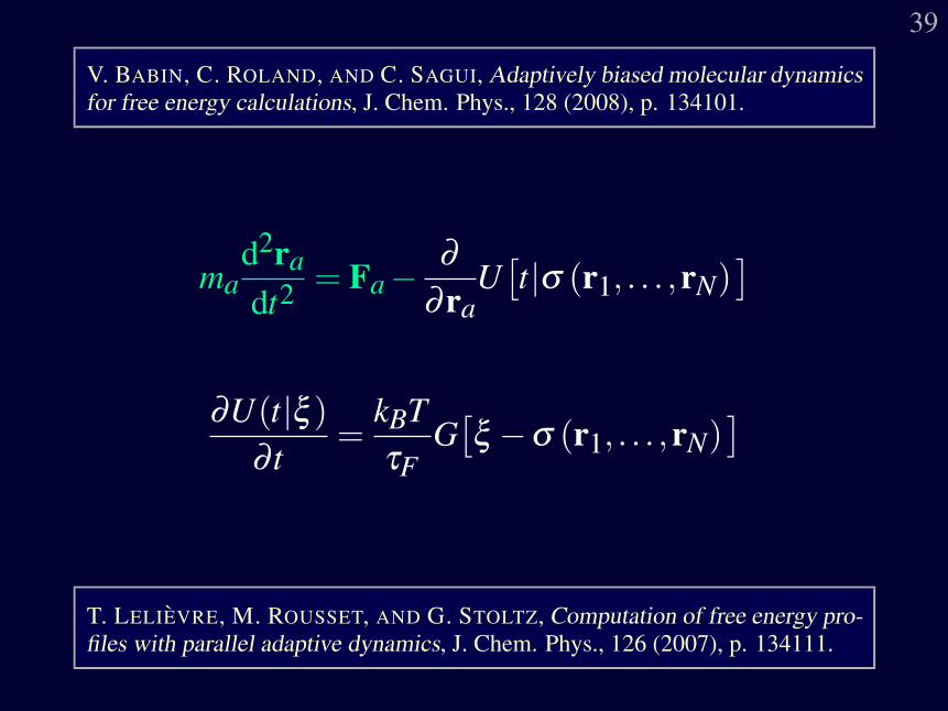
V. BABIN, C. ROLAND, AND C. SAGUI, Adaptively biased molecular dynamicsfor free energy calculations, J. Chem. Phys., 128 (2008), p. 134101.

mad2ra

dt2 = Fa−∂

∂raU[t|σ (r1, . . . ,rN)

]∂U(t|ξ )

∂ t=

kBTτF

G[ξ −σ (r1, . . . ,rN)

]

T. LELIEVRE, M. ROUSSET, AND G. STOLTZ, Computation of free energy pro-files with parallel adaptive dynamics, J. Chem. Phys., 126 (2007), p. 134111.

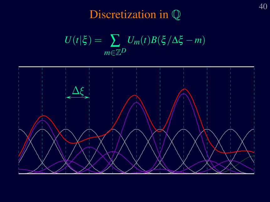
40Discretization in Q

U(t|ξ ) = ∑m∈ZD

Um(t)B(ξ/∆ξ −m)

41

Discretization in Time

Um(t +∆t) = Um(t)+∆tkBTτF

G[σ(t)/∆ξ −m

]

G(ξ ) =4841

(

1− ξ 2/

4)2

, −2≤ ξ ≤ 20, otherwise

42

Advantages of the ABMD

• It is fast: goes as O(t) since the numerical cost ofthe U(t|ξ ) does not depend on time t (it is O(1)).

• It is memory efficient (if sparse arrays are usedfor the Um(t)).

• It is convenient (only two parameters: ∆ξ and τF).

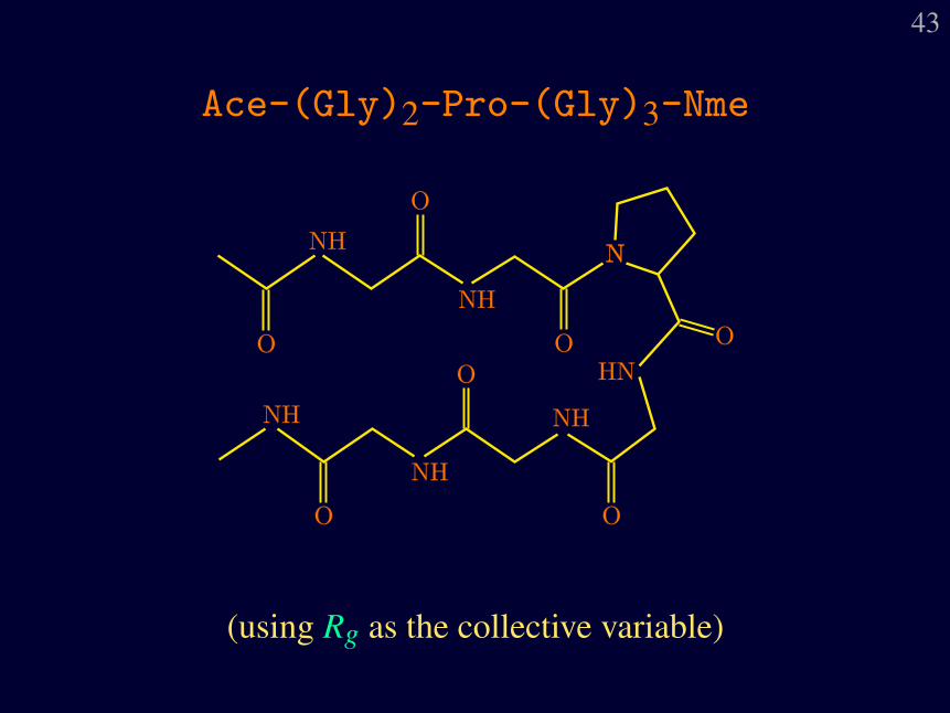
43

Ace-(Gly)2-Pro-(Gly)3-Nme

(using Rg as the collective variable)

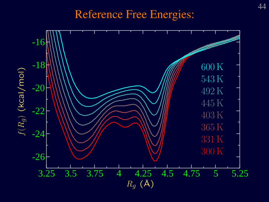
44Reference Free Energies:

3.25 3.5 3.75 4 4.25 4.5 4.75 5 5.25

-26

-24

-22

-20

-18

-16

Rg (A)

f(R

g)(k

cal/

mol) 600 K

543 K492 K445 K403 K365 K331 K300 K

45

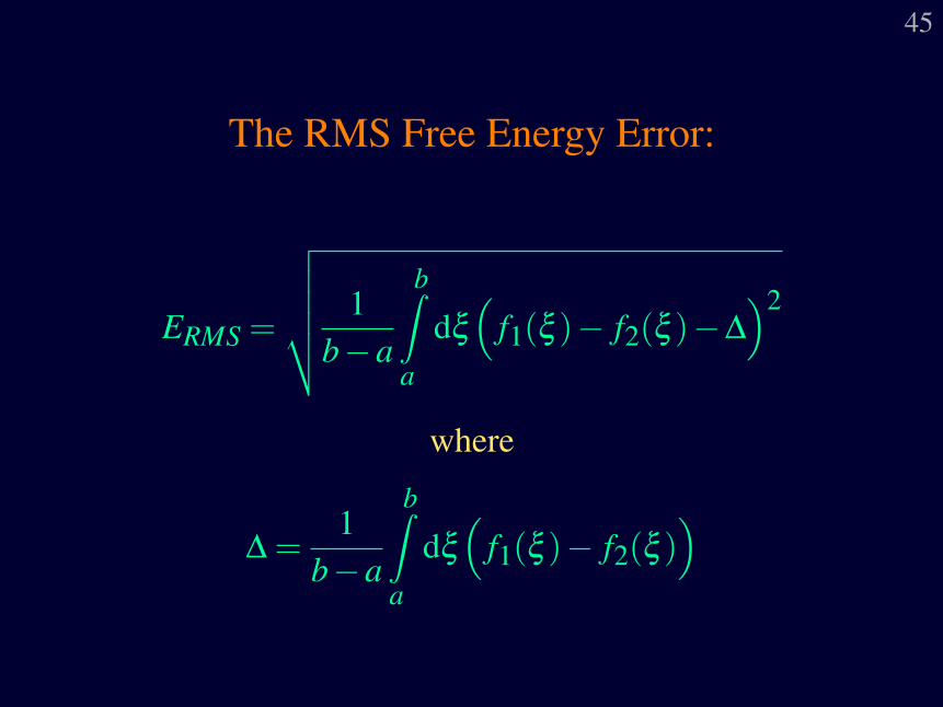
The RMS Free Energy Error:

ERMS =

√√√√√ 1b−a

b∫a

dξ

(f1(ξ )− f2(ξ )−∆

)2

where

∆ =1

b−a

b∫a

dξ

(f1(ξ )− f2(ξ )

)

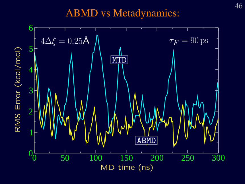
46ABMD vs Metadynamics:

0 50 100 150 200 250 3000

1

2

3

4

5

6

MD time (ns)

RM

SErr

or

(kcal/

mol)

MTD

ABMD

τF = 90 ps4∆ξ = 0.25A

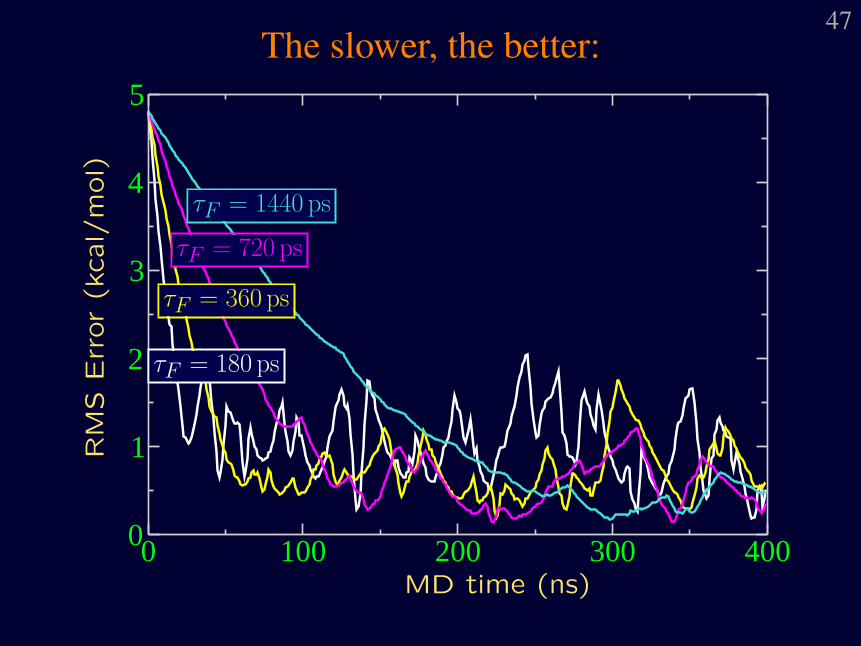
47The slower, the better:

0 100 200 300 4000

1

2

3

4

5

MD time (ns)

RM

SErr

or

(kcal/

mol)

τF = 180 ps

τF = 360 ps

τF = 720 ps

τF = 1440 ps

48

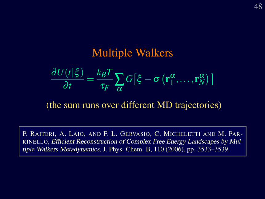
Multiple Walkers

∂U(t|ξ )∂ t

=kBTτF

∑α

G[ξ −σ

(rα

1 , . . . ,rαN)]

(the sum runs over different MD trajectories)

P. RAITERI, A. LAIO, AND F. L. GERVASIO, C. MICHELETTI AND M. PAR-RINELLO, Efficient Reconstruction of Complex Free Energy Landscapes by Mul-tiple Walkers Metadynamics, J. Phys. Chem. B, 110 (2006), pp. 3533–3539.

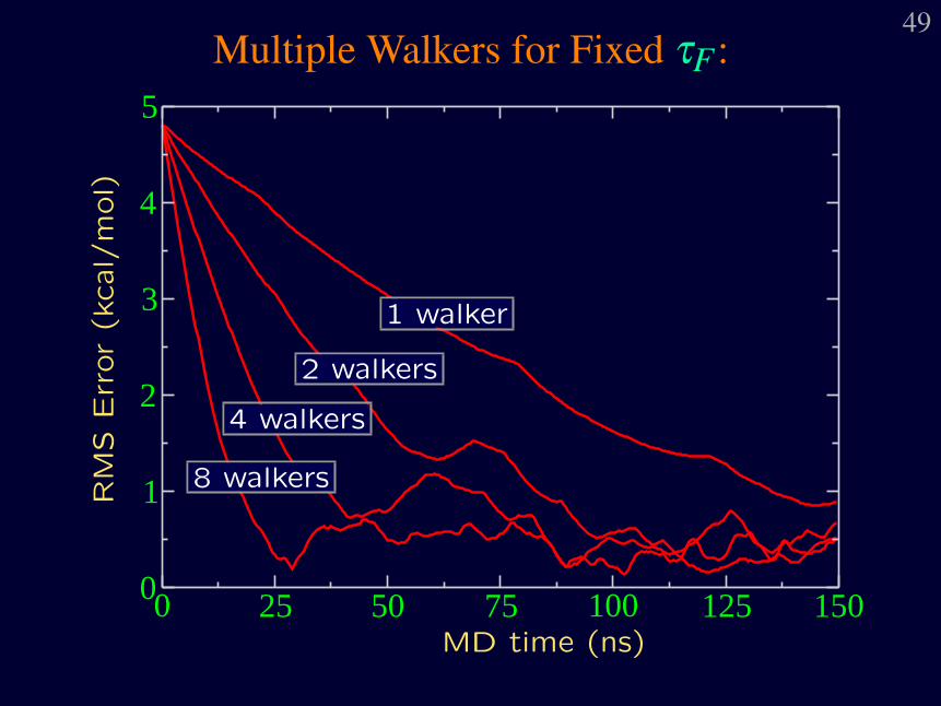
49Multiple Walkers for Fixed τF :

0 25 50 75 100 125 1500

1

2

3

4

5

MD time (ns)

RM

SErr

or

(kcal/

mol)

8 walkers

4 walkers

2 walkers

1 walker

50

Replica Exchange – A Better “Sampling Device”

Y. SUGITA, A. KITAO AND Y. OKAMOTO, Multidimensional replica-exchangemethod for free-energy calculations, J. Chem. Phys., 113 (2000), pp. 6042–6051.

51

• N copies (replicas) in parallel.

• Each replica may have different temperature

and/or collective variable.

• Either stationary (τF = ∞) or evolving biasing

potential on per-replica basis.

52Exchange Probability:

w(m|n) ={

1, ∆≤ 0exp(−∆), ∆ > 0

∆=(

1kBTn

− 1kBTm

)(Em

p −Enp

)+

1kBTm

[Um(ξ n)−Um(ξ m)

]− 1

kBTn

[Un(ξ n)−Un(ξ m)

]

53

Parallel Tempering ABMD

• Different temperatures.

• Same collective variable(s) in all replicas.

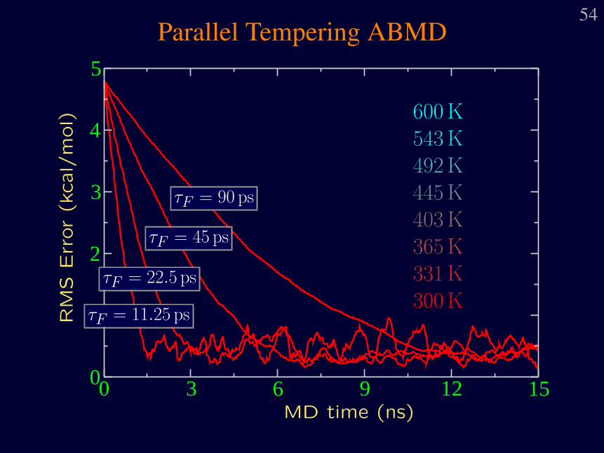
54Parallel Tempering ABMD

0 3 6 9 12 150

1

2

3

4

5

MD time (ns)

RM

SErr

or

(kcal/

mol)

τF = 11.25 ps

τF = 22.5 ps

τF = 45 ps

τF = 90 ps

600 K

543 K

492 K

445 K

403 K

365 K

331 K

300 K

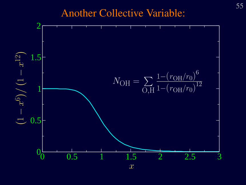
55Another Collective Variable:

0 0.5 1 1.5 2 2.5 30

0.5

1

1.5

2

x

(

1−

x6)

/(

1−

x12

)

NOH =∑

O,H

1−(rOH/r0)6

1−(rOH/r0)12

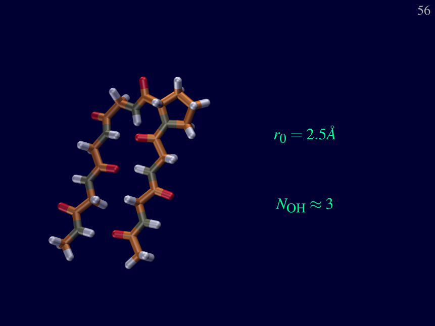
56

r0 = 2.5A

NOH ≈ 3

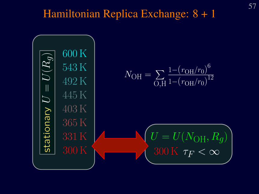
57Hamiltonian Replica Exchange: 8 + 1

600 K

543 K

492 K

445 K

403 K

365 K

331 K

300 Kstationary

U=

U(R

g)

300 K τF < ∞

U = U(NOH, Rg)

NOH =∑

O,H

1−(rOH/r0)6

1−(rOH/r0)12

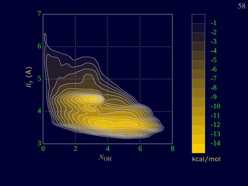
58

3

4

5

6

7

0 2 4 6 8-14-13-12-11-10-9-8-7-6-5-4-3-2-1

NOH

Rg

(A)

kcal/mol

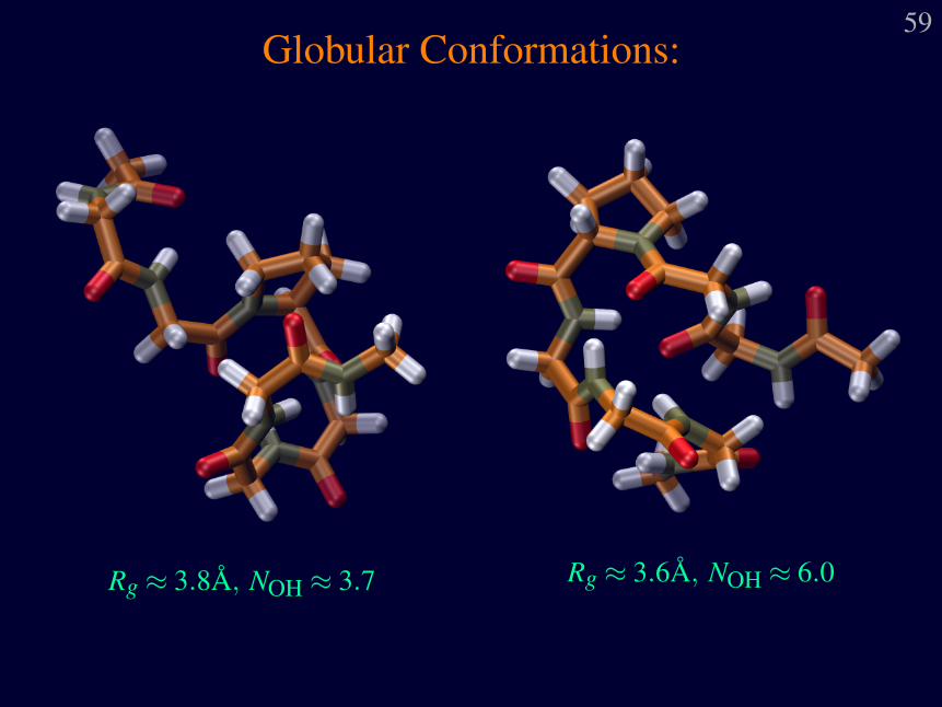
59Globular Conformations:

Rg ≈ 3.8A, NOH ≈ 3.7 Rg ≈ 3.6A, NOH ≈ 6.0

60

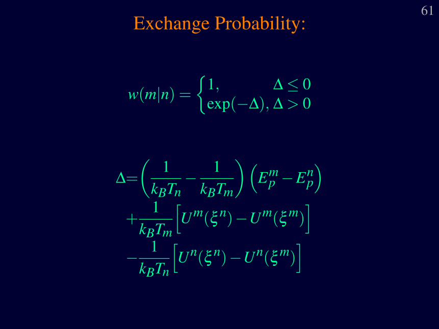
61Exchange Probability:

w(m|n) ={

1, ∆≤ 0exp(−∆), ∆ > 0

∆=(

1kBTn

− 1kBTm

)(Em

p −Enp

)+

1kBTm

[Um(ξ n)−Um(ξ m)

]− 1

kBTn

[Un(ξ n)−Un(ξ m)

]

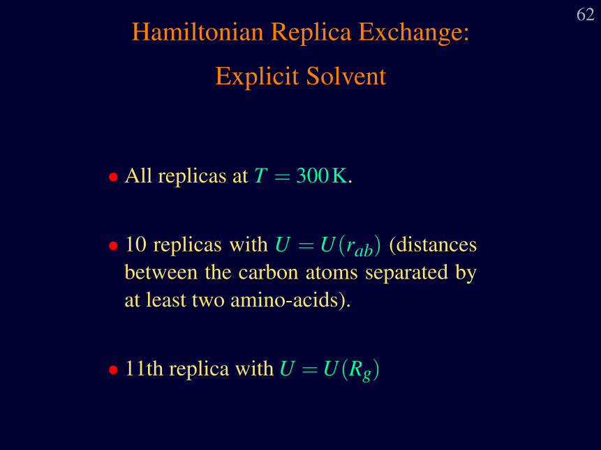
62Hamiltonian Replica Exchange:

Explicit Solvent

• All replicas at T = 300K.

• 10 replicas with U = U(rab) (distancesbetween the carbon atoms separated byat least two amino-acids).

• 11th replica with U = U(Rg)

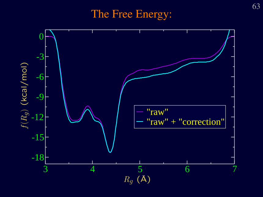
63The Free Energy:

3 4 5 6 7-18

-15

-12

-9

-6

-3

0

"raw""raw" + "correction"

Rg (A)

f(R

g)(k

cal/

mol)

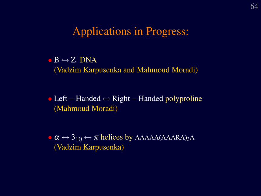
64

Applications in Progress:

• B↔ Z DNA(Vadzim Karpusenka and Mahmoud Moradi)

• Left−Handed↔ Right−Handed polyproline(Mahmoud Moradi)

• α ↔ 310 ↔ π helices by AAAAA(AAARA)3A(Vadzim Karpusenka)

65

The ABMD is included in AMBER 10

(and freely available for AMBER 9)

66Collaborators:

NCSUVolodymyr Babin

Christopher RolandCeleste Sagui

NIEHSThomas Darden

NCSU (students)Vadzim KarpusenkaMahmoud Moradi