Adaptive lasso, MCP, and SCAD - myweb.uiowa.edu · Adaptive lasso Concave penalties Introduction...
34
Adaptive lasso Concave penalties Adaptive lasso, MCP, and SCAD Patrick Breheny February 29 Patrick Breheny High-Dimensional Data Analysis (BIOS 7600) 1/34
Transcript of Adaptive lasso, MCP, and SCAD - myweb.uiowa.edu · Adaptive lasso Concave penalties Introduction...
Adaptive lassoConcave penalties
Adaptive lasso, MCP, and SCAD
Patrick Breheny
February 29
Patrick Breheny High-Dimensional Data Analysis (BIOS 7600) 1/34
Adaptive lassoConcave penalties
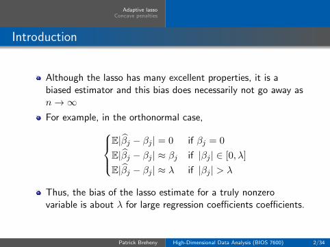
Introduction
Although the lasso has many excellent properties, it is abiased estimator and this bias does necessarily not go away asn→∞For example, in the orthonormal case,
E|βj − βj | = 0 if βj = 0
E|βj − βj | ≈ βj if |βj | ∈ [0, λ]
E|βj − βj | ≈ λ if |βj | > λ
Thus, the bias of the lasso estimate for a truly nonzerovariable is about λ for large regression coefficients coefficients.
Patrick Breheny High-Dimensional Data Analysis (BIOS 7600) 2/34
Adaptive lassoConcave penalties
Adaptive lasso: Motivation
Given that the bias of the estimate is determined by λ, oneapproach to reducing the bias of the lasso is to use theweighted penalty approach we saw last time: λj = wjλ
If one was able to choose the weights such that the variableswith large coefficients had smaller weights, then we couldreduce the estimation bias of the lasso while retaining itssparsity property
Indeed, by more accurately estimating β, one would even beable to improve on the variable selection accuracy of the lasso
Patrick Breheny High-Dimensional Data Analysis (BIOS 7600) 3/34
Adaptive lassoConcave penalties
Adaptive lasso: Motivation (cont’d)
All of this may seem circular in the sense that if we alreadyknew which regression coefficients were large and which weresmall, we wouldn’t need to be carrying out a regressionanalysis in the first place
However, it turns out that the choice of w does not need to beterribly precise in order to realize benefits from this approach
In practice, one can obtain reasonable values for w from anyconsistent initial estimator of β
Patrick Breheny High-Dimensional Data Analysis (BIOS 7600) 4/34
Adaptive lassoConcave penalties
Adaptive lasso
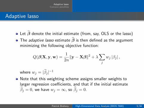
Let β denote the initial estimate (from, say, OLS or the lasso)
The adaptive lasso estimate β is then defined as the argumentminimizing the following objective function:
Q(β|X,y,w) =1
2n‖y −Xβ‖2 + λ
∑j
wj |βj | ,
where wj = |βj |−1
Note that this weighting scheme assigns smaller weights tolarger regression coefficients, and that if the initial estimateβj = 0, we have wj =∞, so βj = 0.
Patrick Breheny High-Dimensional Data Analysis (BIOS 7600) 5/34
Adaptive lassoConcave penalties
Two-stage vs. pathwise approaches
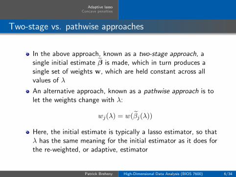
In the above approach, known as a two-stage approach, asingle initial estimate β is made, which in turn produces asingle set of weights w, which are held constant across allvalues of λ
An alternative approach, known as a pathwise approach is tolet the weights change with λ:
wj(λ) = w(βj(λ))
Here, the initial estimate is typically a lasso estimator, so thatλ has the same meaning for the initial estimator as it does forthe re-weighted, or adaptive, estimator
Patrick Breheny High-Dimensional Data Analysis (BIOS 7600) 6/34

Adaptive lassoConcave penalties
Alternative weighting strategies
There are many possibilities besides wj = |βj |−1 for choosingweights based on initial estimates
Really, any nonincreasing function w(β) would be areasonable way to choose weights, and could be used in eithera two-stage or adaptive approach, although the resultingestimators may be quite different
For example, one might allow wj = |βj |−γ or
wj = 1{|βj | > τ}
Patrick Breheny High-Dimensional Data Analysis (BIOS 7600) 7/34
Adaptive lassoConcave penalties
Hybrid and relaxed lasso approaches
A more extreme weighting scheme is
wj =
{0 if βj 6= 0,
∞ if βj = 0
When applied in a two-stage fashion, this approach is knownas the lasso-OLS hybrid estimator (i.e., we use the lasso forvariable selection and OLS for estimation)
When the approach is applied in a pathwise fashion, it isknown as the relaxed lasso
Patrick Breheny High-Dimensional Data Analysis (BIOS 7600) 8/34
Adaptive lassoConcave penalties
SCAD and MCPSolutions in the orthonormal caseSolution pathsThe effect of γ
Single-stage approaches to bias reduction
The adaptive lasso consists of a two-stage approach involvingan initial estimator to reduce bias for large regressioncoefficients
An alternative single-stage approach is to use a penalty thattapers off as β becomes larger in absolute value
Unlike the absolute value penalty employed by the lasso, atapering penalty cannot be convex
Patrick Breheny High-Dimensional Data Analysis (BIOS 7600) 9/34
Adaptive lassoConcave penalties
SCAD and MCPSolutions in the orthonormal caseSolution pathsThe effect of γ
Folded concave penalties
Rather, the penalty function P (β|λ) will be concave withrespect to |β|Such functions are often referred to as folded concavepenalties, to clarify that while P (·) itself is neither convex norconcave, it is concave on both the positive and negativehalves of the real line, and also symmetric (or folded) due toits dependence on the absolute value
Patrick Breheny High-Dimensional Data Analysis (BIOS 7600) 10/34
Adaptive lassoConcave penalties
SCAD and MCPSolutions in the orthonormal caseSolution pathsThe effect of γ
Objective function for folded concave penalties
Consider the objective function
Q(β|X,y) = 1
2n‖y −Xβ‖2 +
p∑j=1
P (βj |λ, γ),
where P (β|λ, γ) is a folded concave penalty
Unlike the lasso, many concave penalties depend on λ in anon-multiplicative way, so that P (β|λ) 6= λP (β)
Furthermore, they typically involve a tuning parameter γ thatcontrols the concavity of the penalty (i.e., how rapidly thepenalty tapers off)
Patrick Breheny High-Dimensional Data Analysis (BIOS 7600) 11/34
Adaptive lassoConcave penalties
SCAD and MCPSolutions in the orthonormal caseSolution pathsThe effect of γ
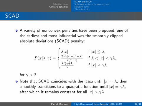
SCAD
A variety of nonconvex penalties have been proposed; one ofthe earliest and most influential was the smoothly clippedabsolute deviations (SCAD) penalty:
P (x|λ, γ) =
λ|x| if |x| ≤ λ,2γλ|x|−x2−λ2
2(γ−1) if λ < |x| < γλ,λ2(γ+1)
2 if |x| ≥ γλ
for γ > 2
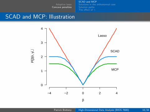
Note that SCAD coincides with the lasso until |x| = λ, thensmoothly transitions to a quadratic function until |x| = γλ,after which it remains constant for all |x| > γλ
Patrick Breheny High-Dimensional Data Analysis (BIOS 7600) 12/34
Adaptive lassoConcave penalties
SCAD and MCPSolutions in the orthonormal caseSolution pathsThe effect of γ
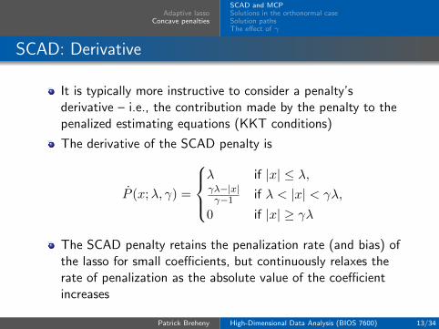
SCAD: Derivative
It is typically more instructive to consider a penalty’sderivative – i.e., the contribution made by the penalty to thepenalized estimating equations (KKT conditions)
The derivative of the SCAD penalty is
P (x;λ, γ) =
λ if |x| ≤ λ,γλ−|x|γ−1 if λ < |x| < γλ,
0 if |x| ≥ γλ
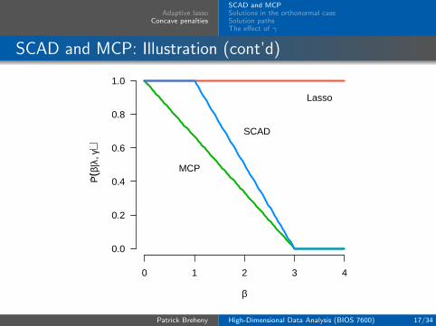
The SCAD penalty retains the penalization rate (and bias) ofthe lasso for small coefficients, but continuously relaxes therate of penalization as the absolute value of the coefficientincreases
Patrick Breheny High-Dimensional Data Analysis (BIOS 7600) 13/34
Adaptive lassoConcave penalties
SCAD and MCPSolutions in the orthonormal caseSolution pathsThe effect of γ
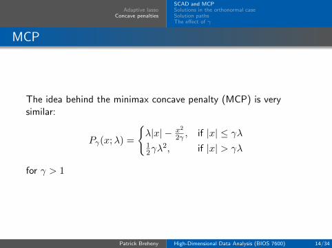
MCP
The idea behind the minimax concave penalty (MCP) is verysimilar:
Pγ(x;λ) =
{λ|x| − x2
2γ , if |x| ≤ γλ12γλ
2, if |x| > γλ
for γ > 1
Patrick Breheny High-Dimensional Data Analysis (BIOS 7600) 14/34
Adaptive lassoConcave penalties
SCAD and MCPSolutions in the orthonormal caseSolution pathsThe effect of γ
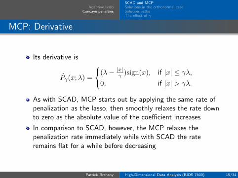
MCP: Derivative
Its derivative is
Pγ(x;λ) =
{(λ− |x|γ )sign(x), if |x| ≤ γλ,0, if |x| > γλ.
As with SCAD, MCP starts out by applying the same rate ofpenalization as the lasso, then smoothly relaxes the rate downto zero as the absolute value of the coefficient increases
In comparison to SCAD, however, the MCP relaxes thepenalization rate immediately while with SCAD the rateremains flat for a while before decreasing
Patrick Breheny High-Dimensional Data Analysis (BIOS 7600) 15/34
Adaptive lassoConcave penalties
SCAD and MCPSolutions in the orthonormal caseSolution pathsThe effect of γ
SCAD and MCP: Illustration
−4 −2 0 2 4
0
1
2
3
4
β
P(β
|λ, γ
)Lasso
SCAD
MCP
Patrick Breheny High-Dimensional Data Analysis (BIOS 7600) 16/34
Adaptive lassoConcave penalties
SCAD and MCPSolutions in the orthonormal caseSolution pathsThe effect of γ
SCAD and MCP: Illustration (cont’d)
0 1 2 3 4
0.0
0.2
0.4
0.6
0.8
1.0
β
P⋅ (β|λ
, γ)
Lasso
SCAD
MCP
Patrick Breheny High-Dimensional Data Analysis (BIOS 7600) 17/34
Adaptive lassoConcave penalties
SCAD and MCPSolutions in the orthonormal caseSolution pathsThe effect of γ
Remarks
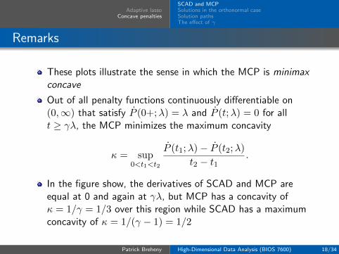
These plots illustrate the sense in which the MCP is minimaxconcave
Out of all penalty functions continuously differentiable on(0,∞) that satisfy P (0+;λ) = λ and P (t;λ) = 0 for allt ≥ γλ, the MCP minimizes the maximum concavity
κ = sup0<t1<t2
P (t1;λ)− P (t2;λ)t2 − t1
.
In the figure show, the derivatives of SCAD and MCP areequal at 0 and again at γλ, but MCP has a concavity ofκ = 1/γ = 1/3 over this region while SCAD has a maximumconcavity of κ = 1/(γ − 1) = 1/2
Patrick Breheny High-Dimensional Data Analysis (BIOS 7600) 18/34
Adaptive lassoConcave penalties
SCAD and MCPSolutions in the orthonormal caseSolution pathsThe effect of γ
MCP & firm thresholding
As with the lasso, MCP and SCAD have closed-form solutionsin the orthonormal case that provide insight into how themethods work
For MCP, the univariate solution is known as the firmthresholding operator:
F (z|λ, γ) =
{γγ−1S(z|λ) if |z| ≤ γλ,
z if |z| > γλ,
where z = x′y/n denotes the unpenalized (OLS) solution
Patrick Breheny High-Dimensional Data Analysis (BIOS 7600) 19/34
Adaptive lassoConcave penalties
SCAD and MCPSolutions in the orthonormal caseSolution pathsThe effect of γ
Remarks: Firm thresholding
As γ →∞, the firm thresholding operator becomes equivalentto the soft thresholding operator: F (z|λ, γ)→ S(z|λ)As γ → 1, it becomes equivalent to hard thresholding
Thus, as γ changes, the solution bridges the gap between softand hard thresholding; hence the name “firm thresholding”
Patrick Breheny High-Dimensional Data Analysis (BIOS 7600) 20/34
Adaptive lassoConcave penalties
SCAD and MCPSolutions in the orthonormal caseSolution pathsThe effect of γ
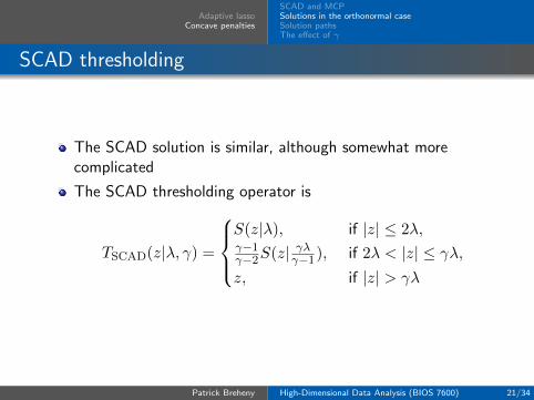
SCAD thresholding
The SCAD solution is similar, although somewhat morecomplicated
The SCAD thresholding operator is
TSCAD(z|λ, γ) =
S(z|λ), if |z| ≤ 2λ,γ−1γ−2S(z|
γλγ−1), if 2λ < |z| ≤ γλ,
z, if |z| > γλ
Patrick Breheny High-Dimensional Data Analysis (BIOS 7600) 21/34
Adaptive lassoConcave penalties
SCAD and MCPSolutions in the orthonormal caseSolution pathsThe effect of γ
Remarks: SCAD thresholding
As with MCP, TSCAD(·|λ, γ)→ S(·|λ) as γ →∞However, as γ → 2, TSCAD(·|λ, γ) does not converge to hardthresholding; instead, it converges to{
S(z;λ), if |z| ≤ 2λ,
z, if |z| > 2λ
In other words, both TSCAD and F converge to discontinuousfunctions as γ approaches its minimum value: for the firmthresholding operator F , the solution jumps from 0 to λ as zexceeds λ, while for the SCAD thresholding operator TSCAD,the solution jumps from λ to 2λ as z exceeds 2λ
Patrick Breheny High-Dimensional Data Analysis (BIOS 7600) 22/34
Adaptive lassoConcave penalties
SCAD and MCPSolutions in the orthonormal caseSolution pathsThe effect of γ
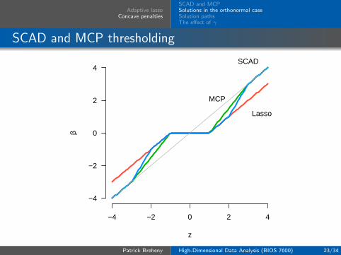
SCAD and MCP thresholding
−4 −2 0 2 4
−4
−2
0
2
4
z
β
Lasso
SCAD
MCP
Patrick Breheny High-Dimensional Data Analysis (BIOS 7600) 23/34
Adaptive lassoConcave penalties
SCAD and MCPSolutions in the orthonormal caseSolution pathsThe effect of γ
Solution paths
To get a sense of how the MCP, SCAD, and adaptive lassoestimates compare to those of the regular lasso, we considerhere the solution paths for the four penalties fit to the samedata
We generate data from the linear regression model
yi =
1000∑j=1
xijβj + εi, i = 1, . . . , 200,
where (β1, . . . , β4) = (4, 2,−4,−2) and the remainingcoefficients are zero
Patrick Breheny High-Dimensional Data Analysis (BIOS 7600) 24/34
Adaptive lassoConcave penalties
SCAD and MCPSolutions in the orthonormal caseSolution pathsThe effect of γ
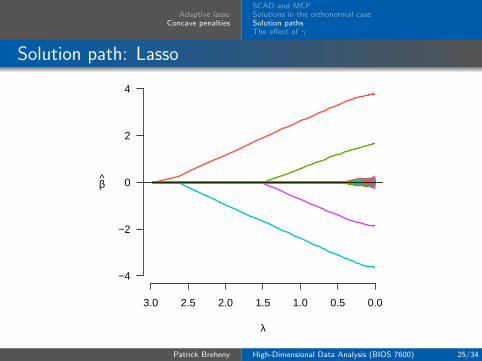
Solution path: Lasso
3.0 2.5 2.0 1.5 1.0 0.5 0.0
−4
−2
0
2
4
λ
β
Patrick Breheny High-Dimensional Data Analysis (BIOS 7600) 25/34
Adaptive lassoConcave penalties
SCAD and MCPSolutions in the orthonormal caseSolution pathsThe effect of γ
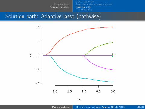
Solution path: Adaptive lasso (pathwise)
2.0 1.5 1.0 0.5 0.0
−4
−2
0
2
4
λ
β
Patrick Breheny High-Dimensional Data Analysis (BIOS 7600) 26/34
Adaptive lassoConcave penalties
SCAD and MCPSolutions in the orthonormal caseSolution pathsThe effect of γ
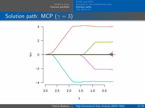
Solution path: MCP (γ = 3)
3.0 2.5 2.0 1.5 1.0 0.5
−4
−2
0
2
4
λ
β
Patrick Breheny High-Dimensional Data Analysis (BIOS 7600) 27/34
Adaptive lassoConcave penalties
SCAD and MCPSolutions in the orthonormal caseSolution pathsThe effect of γ
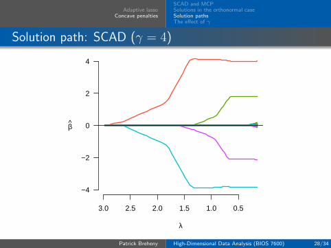
Solution path: SCAD (γ = 4)
3.0 2.5 2.0 1.5 1.0 0.5
−4
−2
0
2
4
λ
β
Patrick Breheny High-Dimensional Data Analysis (BIOS 7600) 28/34
Adaptive lassoConcave penalties
SCAD and MCPSolutions in the orthonormal caseSolution pathsThe effect of γ
Remarks
The primary way in which adaptive lasso, SCAD, and MCPdiffer from the lasso is that they allow the estimatedcoefficients to reach large values more quickly than the lasso
In other words, although the methods all shrink most of thecoefficients towards zero, MCP, SCAD, and the adaptive lassoapply less shrinkage to the nonzero coefficients; this is whatwe refer to in the book as bias reduction
Patrick Breheny High-Dimensional Data Analysis (BIOS 7600) 29/34

Adaptive lassoConcave penalties
SCAD and MCPSolutions in the orthonormal caseSolution pathsThe effect of γ
Remarks (cont’d)
In this example, one can clearly see the piecewise componentsof MCP and SCAD
In particular, it is worth noting that both MCP and SCADpossess an interval of λ values over which all the estimates areflat – over this region, the estimates are the same as those ofordinary least squares regression, but with only the fourvariables with nonzero effects included
These estimates are referred to as the oracle estimates
Patrick Breheny High-Dimensional Data Analysis (BIOS 7600) 30/34
Adaptive lassoConcave penalties
SCAD and MCPSolutions in the orthonormal caseSolution pathsThe effect of γ
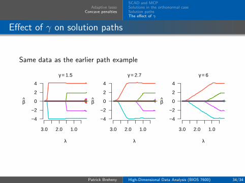
The role of γ in SCAD and MCP
As discussed previously, the tuning parameter γ for the SCADand MCP estimates controls how fast the penalization rategoes to zero
This, in turn, affects the bias of the estimates as well as thestability of the estimate in the sense that as the penaltybecomes more concave, there is a greater chance for multiplelocal minima to exist
As γ →∞, both the MCP and SCAD penalties converge tothe `1 penalty
As γ approaches its minimum value, bias is minimized, butboth estimates become unstable
Patrick Breheny High-Dimensional Data Analysis (BIOS 7600) 31/34
Adaptive lassoConcave penalties
SCAD and MCPSolutions in the orthonormal caseSolution pathsThe effect of γ
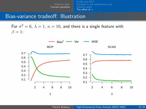
γ and the bias-variance tradeoff
“Stability” here refers to the optimization sense that anobjective function with a single, well-defined minimum isstable while optimization problems with multiple local minimatend are unstable
However, the same remarks apply with respect to thestatistical properties of the estimators, in the sense that amore highly variable estimator is less stable
For SCAD and MCP, lower values of γ produce more highlyvariable, but less biased, estimates
Patrick Breheny High-Dimensional Data Analysis (BIOS 7600) 32/34
Adaptive lassoConcave penalties
SCAD and MCPSolutions in the orthonormal caseSolution pathsThe effect of γ
Bias-variance tradeoff: Illustration
For σ2 = 6, λ = 1, n = 10, and there is a single feature withβ = 1:
2 4 6 8 10
0.1
0.2
0.3
0.4
0.5
0.6
0.7
γ
MCP
2 4 6 8 10
0.1
0.2
0.3
0.4
0.5
0.6
0.7
γ
SCAD
Bias2 Var MSE
Patrick Breheny High-Dimensional Data Analysis (BIOS 7600) 33/34
Adaptive lassoConcave penalties
SCAD and MCPSolutions in the orthonormal caseSolution pathsThe effect of γ
Effect of γ on solution paths
Same data as the earlier path example
3.0 2.0 1.0
−4
−2
0
2
4
λ
β
γ = 1.5
3.0 2.0 1.0
−4
−2
0
2
4
λ
β
γ = 2.7
3.0 2.0 1.0
−4
−2
0
2
4
λ
β
γ = 6
Patrick Breheny High-Dimensional Data Analysis (BIOS 7600) 34/34