The debiased Lasso

Atlanta 2018

Sara van de Geer

The debiased Lasso

Sara van de Geer

August, 2018

The debiased Lasso

Atlanta 2018

Sara van de Geer

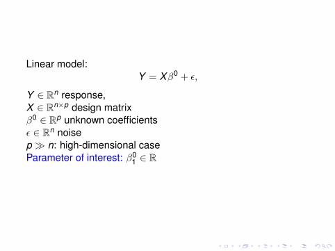
Linear model:Y = Xβ0 + ε,

Y ∈ Rn response,X ∈ Rn×p design matrixβ0 ∈ Rp unknown coefficientsε ∈ Rn noisep � n: high-dimensional caseParameter of interest: β0

1 ∈ R

Assumptions

◦ The rows of (X ,Y ) ∈ Rn×(p+1) are i.i.d.∼ (x,y) ∈ Rp+1

◦ (x,y) is Gaussian with mean zero◦ E(y|x) = xβ0

◦ Σ := ExT x has inverse Θ.◦ ‖Σ‖∞ = O(1), say diag(Σ) = I◦ Λ2

min � 0 where Λ2min is the smallest eigenvalue of Σ

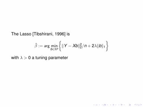
The Lasso [Tibshirani, 1996] is

β := arg minb∈Rp

{‖Y − Xb‖22/n + 2λ‖b‖1

}with λ > 0 a tuning parameter

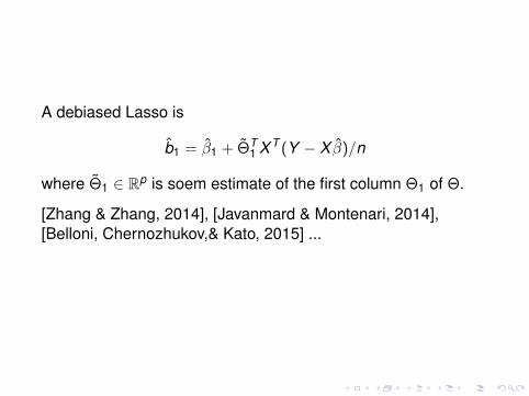
A debiased Lasso is

b1 = β1 + ΘT1 X T (Y − X β)/n

where Θ1 ∈ Rp is soem estimate of the first column Θ1 of Θ.

[Zhang & Zhang, 2014], [Javanmard & Montenari, 2014],[Belloni, Chernozhukov,& Kato, 2015] ...

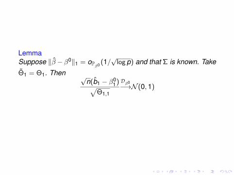
LemmaSuppose ‖β − β0‖1 = oP

β0 (1/√

log p) and that Σ is known. Take

Θ1 = Θ1. Then √n(b1 − β0

1)√Θ1,1

Dβ0−→N (0,1)

Proof.

b1 − β01 = β1 − β0

1 + ΘT1 X T (Y − X β)/n

= β1 − β01 + ΘT

1 X T (ε+ Xβ0︸ ︷︷ ︸=Y

−X β))/n

= β1 − β01︸ ︷︷ ︸

=e1T (β−β0)

+ΘT1 X T ε/n −ΘT

1 X T X/n︸ ︷︷ ︸:=Σ

(β − β0)

= ΘT1 X T ε/n + (e1 − ΣΘ1︸ ︷︷ ︸

=(Σ−Σ)Θ1

)T (β − β0)

We haveΘT

1 X T ε/√

nΘ1,1D−→N (0,1)

where we use ΘT1 ΣΘ1 = ΘT

1 e1 = Θ1,1. Moreover

|((Σ−Σ)Θ1)T (β−β0)| ≤ ‖(Σ− Σ)Θ1‖∞︸ ︷︷ ︸=OP(√

log p/n)

‖β − β0‖1︸ ︷︷ ︸=oP(1/

√log p)

= oP(1/√

n)

tu

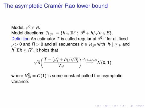
The asymptotic Cramer Rao lower bound

Model: β0 ∈ B.Model directions: Hβ0 := {h ∈ Rp : β0 + h/

√n ∈ B}.

Definition An estimator T is called regular at β0 if for all fixedρ > 0 and R > 0 and all sequences h ∈ Hβ0 with |h1| ≥ ρ andhT Σh ≤ R2, it holds that

√n(

T − (β01 + h1/

√n)

Vβ0

)Dβ0+h/

√n−→ N (0,1)

where V 2β0 = O(1) is some constant called the asymptotic

variance.

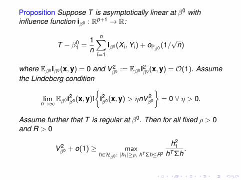
Proposition Suppose T is asymptotically linear at β0 withinfluence function iβ0 : Rp+1 → R:

T − β01 =

1n

n∑i=1

iβ0(Xi ,Yi) + oPβ0 (1/

√n)

where Eβ0 iβ0(x,y) = 0 and V 2β0 := Eβ0 i2

β0(x,y) = O(1). Assumethe Lindeberg condition

limn→∞

Eβ0 i2β0(x,y)l{

i2β0(x,y) > ηnV 2β0

}= 0 ∀ η > 0.

Assume further that T is regular at β0. Then for all fixed ρ > 0and R > 0

V 2β0 + o(1) ≥ max

h∈Hβ0 : |h1|≥ρ, hT Σh≤R2

h21

hT Σh.

Corollary Assume the conditions of the proposition and that forsome fixed ρ > 0 and R > 0 and some sequence h ∈ Hβ0 , with|h1| ≥ ρ and hT Σh ≤ R2, it is true that

V 2β0 =

h21

hT Σh+ o(1).

Then T is asymptotically efficient.

Example Suppose

B := {b ∈ Rp : ‖b‖00︸︷︷︸:=#bj 6=0

≤ s}.

Let S0 := {β0j 6= 0} be the set of active coefficients in β0 and

s0 = |S0|.Some special casesa) If ‖Θ1‖00 ≤ s − s0, then V 2

β0 + o(1) = Θ1,1.b) Suppose {1} ∈ S0, s = s0 and that the following “betamin”condition holds: |β0

j | > mn/√

n for all j ∈ S0, where mn →∞.Then

V 2β0 + o(1) ≥ (Σ−1

S0,S0)1,1.

c) More generally, if {1} ∈ S0 and |β0j | > mn/

√n for all j ∈ S0,

then the lower bound corresponds to knowing the set S0 up tos − s0 additional variables.

Example Suppose

B := {b ∈ Rp : ‖b‖1 ≤√

s}.

Suppose β0 stays away from the boundary of the parameterspace, i.e., for a fixed 0 < η < 1 it holds that‖β0‖1 ≤ (1− η)

√s. Then for all M > 0 fixed

V 2β0 + o(1) ≥

(min

c∈Rp−1: ‖c‖1≤M√

nsE(x1 − x−1c)2

)−1

where x−1 := (x2, . . . ,xp). To improve over Θ1,1 we must havethat Θ1 is rather non-sparse: ‖Θ1‖1 should be of larger orderthan

√ns.

Example Suppose

B := {b ∈ Rp : ‖b‖rr ≤√

s2−r}.

If β0 stays away from the boundary, then for all M > 0 fixed

V 2β0 + o(1) ≥

(min

c∈Rp−1: ‖c‖1≤M√

nr s2−rE(x1 − x−1c)2

)−1

.

To improve over Θ1,1 we must have that ‖Θ1‖1 is of larger orderthan

√nr s2−r .

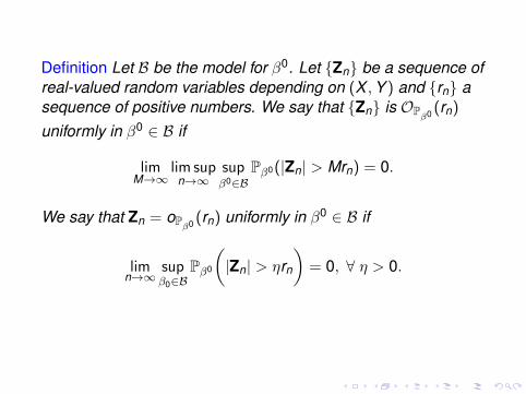
Definition Let B be the model for β0. Let {Zn} be a sequence ofreal-valued random variables depending on (X ,Y ) and {rn} asequence of positive numbers. We say that {Zn} is OP

β0 (rn)

uniformly in β0 ∈ B if

limM→∞

lim supn→∞

supβ0∈B

Pβ0(|Zn| > Mrn) = 0.

We say that Zn = oPβ0 (rn) uniformly in β0 ∈ B if

limn→∞

supβ0∈B

Pβ0

(|Zn| > ηrn

)= 0, ∀ η > 0.

Notationγ0 := arg min

c∈Rp−1E(x1 − x−1c)2.

Remark Thusγ0 = Σ−1

−1,−1ExT−1x1

where Σ−1,−1 := ExT−1x−1, and E(x1|x−1) = x−1γ

0.We say that x−1γ

0 is the projection of x1 on x−1.

The case Σ known

Definition Let γ] ∈ Rp−1 and λ] > 0. We say that the pair(γ], λ]) is eligible if

‖Σ−1,−1(γ] − γ0)‖∞ ≤ λ] (1)

andλ]‖γ]‖1 → 0. (2)

We then define

Θ]1 :=

(1−γ]

)/(1− γ0T Σ−1,−1γ

]). (3)

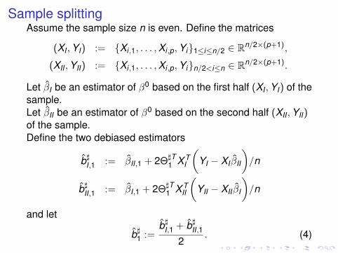
Sample splittingAssume the sample size n is even. Define the matrices

(XI ,YI) := {Xi,1, . . . ,Xi,p,Yi}1≤i≤n/2 ∈ Rn/2×(p+1),

(XII ,YII) := {Xi,1, . . . ,Xi,p,Yi}n/2<i≤n ∈ Rn/2×(p+1).

Let βI be an estimator of β0 based on the first half (XI ,YI) of thesample.Let βII be an estimator of β0 based on the second half (XII ,YII)of the sample.Define the two debiased estimators

b]I,1 := βII,1 + 2Θ]T1 X T

I

(YI − XI βII

)/n

b]II,1 := βI,1 + 2Θ]T1 X T

II

(YII − XII βI

)/n

and let

b]1 :=b]I,1 + b]II,1

2. (4)

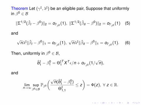
Theorem Let (γ], λ]) be an eligible pair, Suppose that uniformlyin β0 ∈ B

‖Σ1/2(βI − β0)‖2 = oPβ0 (1), ‖Σ1/2(βII − β0)‖2 = oP

β0 (1) (5)

and√

nλ]‖βI − β0‖1 = oPβ0 (1),

√nλ]‖βII − β0‖1 = oP

β0 (1). (6)

Then, uniformly in β0 ∈ B,

b]1 − β01 = Θ]T

1 X T ε/n + oPβ0 (1/

√n),

and

limn→∞

supβ0∈B

Pβ0

(√n(b]1 − β

01)

Θ]1,1

≤ z)

= Φ(z), ∀ z ∈ R.

Corollary The theorem shows that under its conditions theestimator b]1 is uniformly asymptotically linear and regular. Itmeans that for this estimator the Cramer Rao lower bound isrelevant.

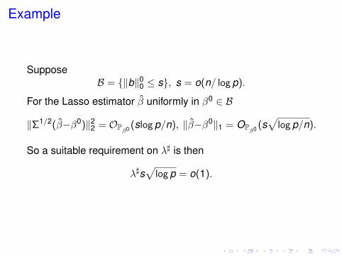
Example

SupposeB = {‖b‖00 ≤ s}, s = o(n/ log p).

For the Lasso estimator β uniformly in β0 ∈ B

‖Σ1/2(β−β0)‖22 = OPβ0 (slog p/n), ‖β−β0‖1 = OP

β0 (s√

log p/n).

So a suitable requirement on λ] is then

λ]s√

log p = o(1).

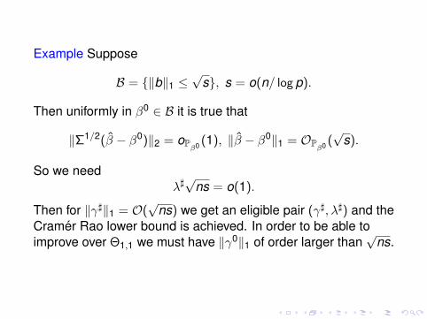
Example Suppose

B = {‖b‖1 ≤√

s}, s = o(n/ log p).

Then uniformly in β0 ∈ B it is true that

‖Σ1/2(β − β0)‖2 = oPβ0 (1), ‖β − β0‖1 = OP

β0 (√

s).

So we needλ]√

ns = o(1).

Then for ‖γ]‖1 = O(√

ns) we get an eligible pair (γ], λ]) and theCramer Rao lower bound is achieved. In order to be able toimprove over Θ1,1 we must have ‖γ0‖1 of order larger than

√ns.

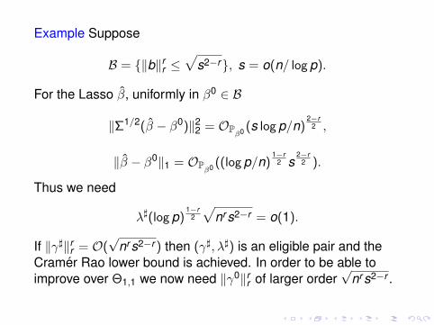
Example Suppose

B = {‖b‖rr ≤√

s2−r}, s = o(n/ log p).

For the Lasso β, uniformly in β0 ∈ B

‖Σ1/2(β − β0)‖22 = OPβ0 (s log p/n)

2−r2 ,

‖β − β0‖1 = OPβ0 ((log p/n)

1−r2 s

2−r2 ).

Thus we need

λ](log p)1−r

2

√nr s2−r = o(1).

If ‖γ]‖rr = O(√

nr s2−r ) then (γ], λ]) is an eligible pair and theCramer Rao lower bound is achieved. In order to be able toimprove over Θ1,1 we now need ‖γ0‖rr of larger order

√nr s2−r .

Σ Σknown known

B = {‖b‖00 ≤ s} B = {‖b‖1 ≤√

s}asymp- s = o( n

log p ) s = o( nlog p )

totic λ]slog12 p = o(1) λ]

√ns = o(1)

norma-lity λ]‖γ]‖1 = o(1) λ]‖γ]‖1 = o(1)

asymp-totic yes yes

linearityasymp-

totic ‖γ]‖00 = O(s) ‖γ]‖1 = O(√

ns)efficiency

Table: Throughout, (γ], λ]) is required to be an eligible pair, i.e.‖Σ−1,−1(γ] − γ0)‖∞ ≤ λ] (and λ]‖γ]‖1 → 0). Asymptotic efficiency isestablished when β0 stays away from the boundary of B. In the caseB = {‖b‖0

0 ≤ s} the conditions on γ] for asymptotic efficiency dependon β0.

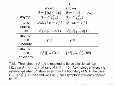
Σ Σknown known

B = {‖b‖00 ≤ s} B = {‖b‖rr ≤√

s2−r}asymp- s = o( n

log p ) s = o( nlog p )

totic λ]slog12 p = o(1) λ]n

r2 s

2−r2 log

1−r2 p = o(1)

norma-lity λ]‖γ]‖1 = o(1) λ]‖γ]‖1 = o(1)

asymp-totic yes yes

linearityasymp-

totic ‖γ]‖00 = O(s) ‖γ]‖rr = O(nr2 s

2−r2 )

efficiency

Table: Throughout, (γ], λ]) is required to be an eligible pair i.e.‖Σ−1,−1(γ] − γ0)‖∞ ≤ λ] (and λ]‖γ]‖1 → 0). Asymptotic efficiency isestablished when β0 stays away from the boundary of B. In the caseB = {‖b‖0

0 ≤ s} the conditions on γ] for asymptotic efficiency dependon β0.

Finding eligible pairs

Remark The pair (γ], λ]) is eligible iff

x−1γ0 = x−1γ

] + ε0,

where |cov(xj , ε0)| ≤ λ] and λ]‖γ]‖1 → 0.

Moreover, Θ1,1 � Θ]1,1 iff E(ε0)2 � 0.

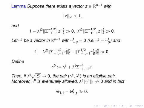
Lemma Suppose there exists a vector z ∈ Rp−1 with

‖z‖∞ ≤ 1,

and1− λ]2‖Σ−1/2

−1,−1z‖22 � 0, λ]2‖Σ−1/2−1,−1z‖22 � 0.

Let γ] be a vector in Rp−1 with γ]−S = 0 (i.e. γ] = γ]S) and

1− λ]2‖Σ−1/2−1,−1z‖22 − ‖Σ

1/2−1,−1γ

]S‖

22 � 0.

Defineγ0 := γ] + λ]Σ−1

−1,−1z.

Then, if λ]√|S| → 0, the pair (γ], λ]) is an eligible pair.

Moreover, γ0 is eventually allowed, λ]‖γ0‖1 6→ 0 and in fact

Θ1,1 −Θ]1,1 � 0.

The case Σ unknown

We use the noisy Lasso

γ ∈ arg minc∈Rp−1

{‖X−1 − X−1c‖22/n + 2λLasso‖c‖1

}. (7)

Then in the debiased Lasso we apply

Θ1 := Θ1

where

Θ1 :=

(1−γ

)/(‖X1 − X−1γ‖22/n + λLasso‖γ‖1). (8)

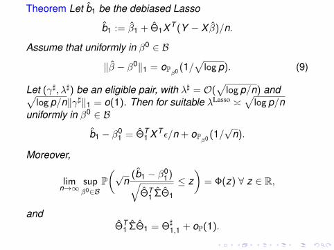
Theorem Let b1 be the debiased Lasso

b1 := β1 + Θ1X T (Y − X β)/n.

Assume that uniformly in β0 ∈ B

‖β − β0‖1 = oPβ0 (1/

√log p). (9)

Let (γ], λ]) be an eligible pair, with λ] = O(√

log p/n) and√log p/n‖γ]‖1 = o(1). Then for suitable λLasso �

√log p/n

uniformly in β0 ∈ B

b1 − β01 = ΘT

1 X T ε/n + oPβ0 (1/

√n).

Moreover,

limn→∞

supβ0∈B

P(√

n(b1 − β0

1)√ΘT

1 ΣΘ1

≤ z)

= Φ(z) ∀ z ∈ R,

andΘT

1 ΣΘ1 = Θ]1,1 + oP(1).

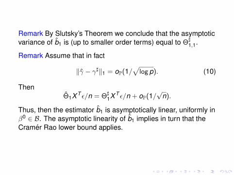
Remark By Slutsky’s Theorem we conclude that the asymptoticvariance of b1 is (up to smaller order terms) equal to Θ]

1,1.

Remark Assume that in fact

‖γ − γ]‖1 = oP(1/√

log p). (10)

ThenΘ1X T ε/n = Θ]

1X T ε/n + oP(1/√

n).

Thus, then the estimator b1 is asymptotically linear, uniformly inβ0 ∈ B. The asymptotic linearity of b1 implies in turn that theCramer Rao lower bound applies.

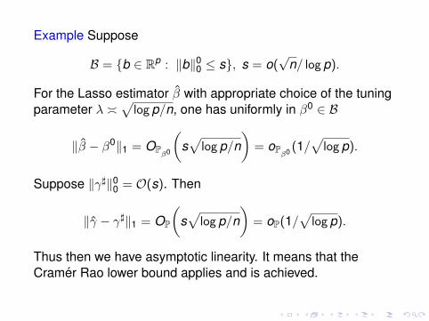
Example Suppose

B = {b ∈ Rp : ‖b‖00 ≤ s}, s = o(√

n/ log p).

For the Lasso estimator β with appropriate choice of the tuningparameter λ �

√log p/n, one has uniformly in β0 ∈ B

‖β − β0‖1 = OPβ0

(s√

log p/n)

= oPβ0 (1/

√log p).

Suppose ‖γ]‖00 = O(s). Then

‖γ − γ]‖1 = OP

(s√

log p/n)

= oP(1/√

log p).

Thus then we have asymptotic linearity. It means that theCramer Rao lower bound applies and is achieved.

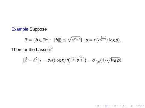
Example Suppose

B = {b ∈ Rp : ‖b‖rr ≤√

s2−r}, s = o(n1−r2−r / log p).

Then for the Lasso β

‖β − β0‖1 = oP((log p/n)1−r

2 s2−r

2 ) = oPβ0 (1/

√log p).

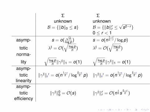
Σ Σunknown unknown

B = {‖b‖0 ≤ s} B = {‖b‖rr ≤√

s2−r}0 ≤ r < 1

asymp- s = o(√

nlog p ) s = o(n

1−r2−r / log p)

totic λ] = O(√

log pn ) λ] = O(

√log p

n )

norma-

lity√

log pn ‖γ

]‖1 = o(1)√

log pn ‖γ

]‖1 = o(1)

asymp-totic ‖γ]‖r

r = o(n1−r

2 / log2−r

2 p) ‖γ]‖rr = o(n

1−r2 / log

2−r2 p)

linearityasymp-

totic ‖γ]‖00 = O(s) ‖γ]‖rr = O(nr2 s

2−r2 )

efficiency

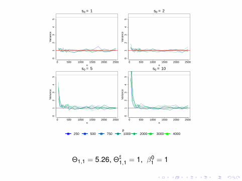
Some simulations ...

Acknowledgement: Francesco Ortelli

0 500 1000 1500 2000 2500

01

23

45

s0 = 1

n

Var

ianc

e

0 500 1000 1500 2000 2500

01

23

45

s0 = 2

n

Var

ianc

e0 500 1000 1500 2000 2500

01

23

45

s0 = 5

n

Var

ianc

e

0 500 1000 1500 2000 2500

01

23

45

s0 = 10

nV

aria

nce

p250 500 750 1000 2000 3000 4000

Θ1,1 = 5.26, Θ]1,1 = 1, β0

1 = 1

0 500 1000 1500 2000 2500

01

23

45

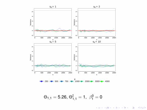
s0 = 1

n

Var

ianc

e

0 500 1000 1500 2000 2500

01

23

45

s0 = 2

n

Var

ianc

e0 500 1000 1500 2000 2500

01

23

45

s0 = 5

n

Var

ianc

e

0 500 1000 1500 2000 2500

01

23

45

s0 = 10

nV

aria

nce

p250 500 750 1000 2000 3000 4000

Θ1,1 = 5.26, Θ]1,1 = 1, β0

1 = 0