A straightforward 2ω technique for themeasurement of the Thomson effect

Isaac Haık DunnSupervisor: Antoine Maignan

Cosupervisors: Ramzy Daou, Mohamed Fall

Normandie Universite, ENSICAEN, CNRS, Crismat-Greensystech

October 18th, 2018

1

Outline

Thermoelectricity and the Thomson effect

Our 2ω methodPhysical descriptionPhysics of the systemGetting µ

Validation of the methodSimulationsSeebeck measurement

Conclusion

2

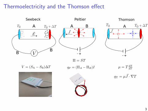
Thermoelectricity and the Thomson effect

+++

-- -

-- --

-- -

+++

+

+++

A

BB

Seebeck Peltier Thomson

BA

+-

A

+-

3

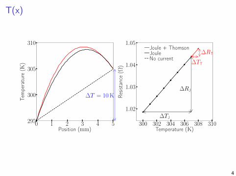
T(x)

0 1 2 3 4 5Position (mm)

295

300

305

310

Temperature

(K)

∆T = 10 K

300 302 304 306 308 310Temperature (K)

1.02

1.03

1.04

1.05

Resis

tance(Ω

)

∆RJ

∆RT

∆TJ

∆TT

Joule + ThomsonJouleNo current

4

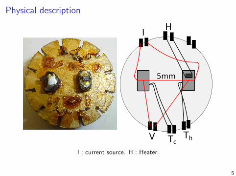
Physical description

I

V

H

ThTc

5mm

I : current source. H : Heater.

5

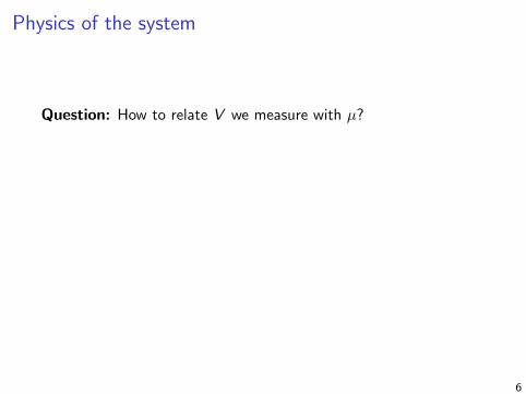
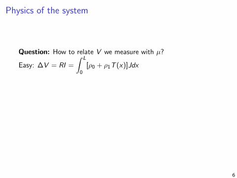
Physics of the system

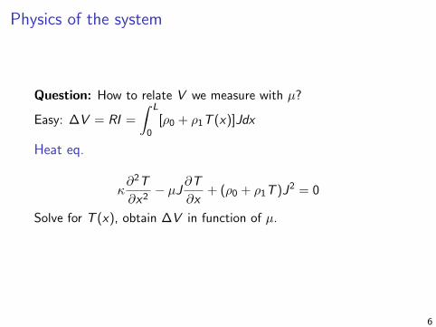
Question: How to relate V we measure with µ?

Easy: ∆V = RI =

∫ L

0[ρ0 + ρ1T (x)]Jdx

Heat eq.

κ∂2T

∂x2− µJ ∂T

∂x+ (ρ0 + ρ1T )J2 = 0

Solve for T (x), obtain ∆V in function of µ.

6

Physics of the system

Question: How to relate V we measure with µ?

Easy: ∆V = RI =

∫ L

0[ρ0 + ρ1T (x)]Jdx

Heat eq.

κ∂2T

∂x2− µJ ∂T

∂x+ (ρ0 + ρ1T )J2 = 0

Solve for T (x), obtain ∆V in function of µ.

6

Physics of the system

Question: How to relate V we measure with µ?

Easy: ∆V = RI =

∫ L

0[ρ0 + ρ1T (x)]Jdx

Heat eq.

κ∂2T

∂x2− µJ ∂T

∂x+ (ρ0 + ρ1T )J2 = 0

Solve for T (x), obtain ∆V in function of µ.

6

Physics of the system - AC method

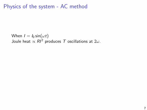
When I = I0 sin(ωt)Joule heat ∝ RI 2 produces T oscillations at 2ω.

Thomson heat ∝ I produces T oscillations at 1ω.We measure V (t).Impact of the T oscillations on V :From Ohm’s law V = RI ≈ (R0 + R1T )I0 sin(ωt)Means V oscillations at 3ω (Joule) and 2ω (Thomson).

7

Physics of the system - AC method

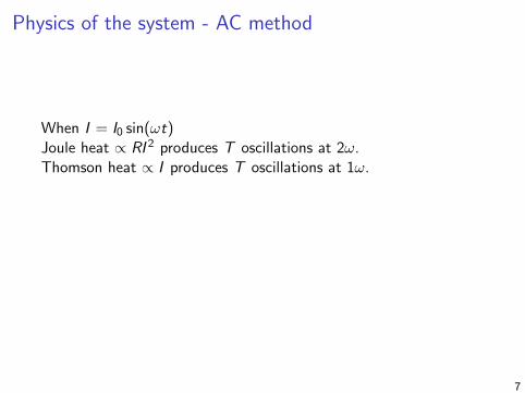
When I = I0 sin(ωt)Joule heat ∝ RI 2 produces T oscillations at 2ω.Thomson heat ∝ I produces T oscillations at 1ω.

We measure V (t).Impact of the T oscillations on V :From Ohm’s law V = RI ≈ (R0 + R1T )I0 sin(ωt)Means V oscillations at 3ω (Joule) and 2ω (Thomson).

7

Physics of the system - AC method

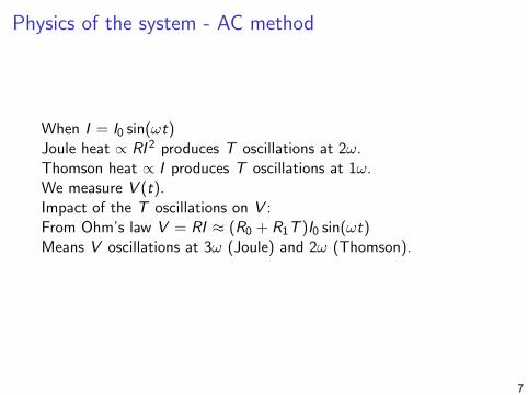
When I = I0 sin(ωt)Joule heat ∝ RI 2 produces T oscillations at 2ω.Thomson heat ∝ I produces T oscillations at 1ω.We measure V (t).Impact of the T oscillations on V :From Ohm’s law V = RI ≈ (R0 + R1T )I0 sin(ωt)Means V oscillations at 3ω (Joule) and 2ω (Thomson).

7

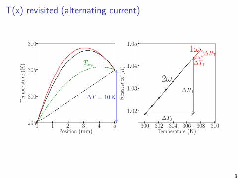
T(x) revisited (alternating current)

0 1 2 3 4 5Position (mm)

295

300

305

310

Temperature

(K)

∆T = 10 K

Tavg.

300 302 304 306 308 310Temperature (K)

1.02

1.03

1.04

1.05

Resis

tance(Ω

)

∆RJ

∆RT

∆TJ

∆TT

2ω

1ω

8

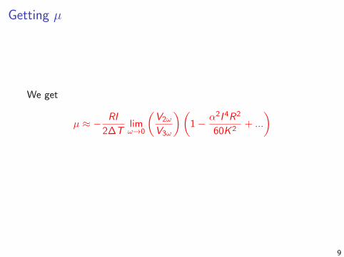
Getting µ

We get

µ ≈ − RI

2∆Tlimω→0

(V2ω

V3ω

)(1− α2I 4R2

60K 2+ ...

)

9

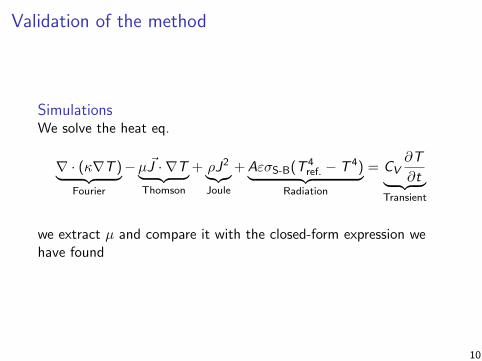
Validation of the method

SimulationsWe solve the heat eq.

∇ · (κ∇T )︸ ︷︷ ︸Fourier

−µ ~J · ∇T︸ ︷︷ ︸Thomson

+ ρJ2︸︷︷︸Joule

+AεσS-B(T 4ref. − T 4)︸ ︷︷ ︸

Radiation

= CV∂T

∂t︸ ︷︷ ︸Transient

we extract µ and compare it with the closed-form expression wehave found

10

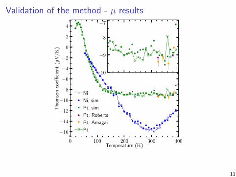
Validation of the method - µ results

0 100 200 300 400Temperature (K)

−16

−14

−12

−10

−8

−6

−4

−2

0

2

4

Tho

msoncoeffi

cient(µ

V/K)

NiNi, simPt, simPt, RobertsPt, AmagaiPt

−10

−9

−8

−7

11

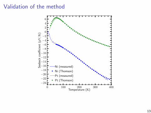
Validation of the method

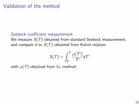
Seebeck coefficient measurementWe measure S(T ) obtained from standard Seebeck measurement,and compare it to S(T ) obtained from Kelvin relation:

S(T ) =

∫ T

0

µ(T ′)

T ′ dT ′

with µ(T ) obtained from 2ω method.

12

Validation of the method

0 100 200 300 400Temperature (K)

−24

−22

−20

−18

−16

−14

−12

−10

−8

−6

−4

−2

0

2

4

6

Seebeckcoeffi

cient(µ

V/K)

Ni (measured)Ni (Thomson)Pt (measured)Pt (Thomson)

13

Conclusion

I We developed a new method to obtain µ with at least±0.5 µV/K. Advantage of being simple, fast, and accurate.Easily extendable to high temperatures (> 1000 K) and othermaterials. Higher accuracy can be achieved by the use oflower frequencies.

I The method was validated through the use of simulations and comparison withSeebeck coefficient measurements.

I We present corrections for κ when the current is high. Very useful for thestandard 3ω method. Similar corrections for µ, though it is much less affected.

I We also give a clue on the impact of radiation effects, µ being very littleimpacted while κ can potentially require corrections at high temperature.

14

Conclusion

I We developed a new method to obtain µ with at least±0.5 µV/K. Advantage of being simple, fast, and accurate.Easily extendable to high temperatures (> 1000 K) and othermaterials. Higher accuracy can be achieved by the use oflower frequencies.

I The method was validated through the use of simulations and comparison withSeebeck coefficient measurements.

I We present corrections for κ when the current is high. Very useful for thestandard 3ω method. Similar corrections for µ, though it is much less affected.

I We also give a clue on the impact of radiation effects, µ being very littleimpacted while κ can potentially require corrections at high temperature.

14

Conclusion

I We developed a new method to obtain µ with at least±0.5 µV/K. Advantage of being simple, fast, and accurate.Easily extendable to high temperatures (> 1000 K) and othermaterials. Higher accuracy can be achieved by the use oflower frequencies.

I The method was validated through the use of simulations and comparison withSeebeck coefficient measurements.

I We present corrections for κ when the current is high. Very useful for thestandard 3ω method. Similar corrections for µ, though it is much less affected.

I We also give a clue on the impact of radiation effects, µ being very littleimpacted while κ can potentially require corrections at high temperature.

14

Conclusion

I We developed a new method to obtain µ with at least±0.5 µV/K. Advantage of being simple, fast, and accurate.Easily extendable to high temperatures (> 1000 K) and othermaterials. Higher accuracy can be achieved by the use oflower frequencies.

I The method was validated through the use of simulations and comparison withSeebeck coefficient measurements.

I We present corrections for κ when the current is high. Very useful for thestandard 3ω method. Similar corrections for µ, though it is much less affected.

I We also give a clue on the impact of radiation effects, µ being very littleimpacted while κ can potentially require corrections at high temperature.

14

The end

Thank you!

Reference: https://arxiv.org/abs/1809.08040

15