European Congress on Computational Methodsin Applied Sciences and Engineering (ECCOMAS 2012)

J. Eberhardsteiner et.al. (eds.)Vienna, Austria, September 10-14, 2012

A PHASE-FIELD TOPOLOGY OPTIMIZATION MODEL USING ADOUBLE-OBSTACLE FUNCTION

Tomohiro Takaki

Mechanical and System Engineering, Graduate School of Science and Technology,Kyoto Institute of Technology,

Matsugasaki, Sakyo, Kyoto 606-85858, Japane-mail: takaki@kit.ac.jp

Keywords: topology optimization, phase-field method, double-obstacle function, stiffness max-imization

Abstract. A phase-field topology optimization model, which maximizes the structure stiffnessunder fixed material volume using a double-obstacle function, has been developed. By usingthe double-obstacle function, the interface region can be defined clearly. By performing two-dimensional simulations for a cantilever model and comparing the results to those obtainedfrom the phase-field topology model with a double-well function, the fundamental characteris-tics of the developed model have been investigated. As a result, although some unstable struc-tures were observed, almost all results coincided with those obtained by a phase-field topologymodel with a double-well function.

Tomohiro Takaki

1 INTRODUCTION

Topology optimization that optimizes material layout, which includes changes in the numberand shape of holes within a given design space, is a method having the highest degree of free-dom among optimization design methods [1]. The level-set method is the method most oftenused to track surface position in topology optimization simulations. Although the phase-fieldmethod is another surface tracking method and is the most powerful numerical method usedin material microstructure design, there are only a few topology optimization models in whichthe phase-field method is used as the surface tracking method instead of the level-set method[2]. In our previous study, we have developed a phase-field topology optimization model thatmaximizes structure stiffness [3]. This model was derived using the same procedure as in amaterial microstructure model and the coefficients used in the phase-field equation were clearlyrelated to the surface energy and surface thickness.

In the present study, we have developed a phase-field topology optimization model using adouble-obstacle function instead of the double-well function used in ordinary phase-field mod-els [2, 3]. By performing two-dimensional simulations for a cantilever model and comparing theresults to those obtained using the phase-field topology model with a double-well function, thefundamental characteristics of the developed model have been confirmed. The double-obstaclefunction is employed in the multiphase-field model [4], for which application to multicompo-nent structure design is anticipated.

2 PHASE-FIELD TOPOLOGY OPTIMIZATION MODEL

In this chapter, by following previous work [3], a phase-field topology optimization modelwith a double-obstacle function is derived together with a model with a double-well function.Hereafter, the phase-field topology optimization models with double-well and double-obstaclefunctions are referred to as “Model I” and “Model II,” respectively.

The phase-field variable φ is defined as φ = 1 in solid and φ = 0 in vapor (or hole) andchanges smoothly and rapidly at the surface region. The free energy functional that maximizesthe structure stiffness under a constant volume can be described as

F = Fm + Fp − Ff , (1)

where Fm is the free energy in bulk, Fp is the penalty energy to keep a constant volume, and Ff

is the external force potential. These are expressed as

Fm =∫

VfdV =

∫V

(fgrad + fdoub − felast) dV , (2)

Fp = k |V − V0| , (3)

Ff = −∫

Suip̄idS. (4)

In Eq. (2), the gradient energy density fgrad, the double-well potential fdoub, and the elasticstrain energy felast are described as follows:

fgrad =a2

2|∇φ|2 , (5)

fdoub = Wq (φ) , (6)

felast =1

2Cijkl (φ) εijεkl =

1

2Cijklεijεklρ (φ) . (7)

2

Tomohiro Takaki

Here, a is the gradient coefficient, W is the energy barrier, εij is the strain tensor, and Cijkl isthe elastic coefficient tensor. q (φ) is the double-well or double-obstacle function and ρ (φ) isthe solid density function. For q (φ) and ρ (φ), we chose the following two types of function:

Model I:q (φ) = φ2 (1 − φ)2 , (8)

ρ (φ) = φ3(10 − 15φ + 6φ2

); (9)

Model II:q (φ) = φ (1 − φ) , (10)

ρ (φ) =8

π

{1

4(2φ − 1)

√φ (1 − φ) +

1

8arcsin (2φ − 1)

}+

1

2. (11)

Figure 1 shows the profiles of q(φ) and ρ(φ) for Model I (solid line) and Model II (broken line).For q(φ), Eq. (8) and Eq. (10) are multiplied by 16 and 4, respectively, to set those maximumvalues to one.

ρ(φ)

0.0

1.0 4q(φ) Model II

16q(φ) Model I0.5

0.0

1.0

0.5

q(φ)

Model IIModel I

0.0 1.00.5φ

0.0 1.00.5φ

Figure 1: Profiles of q(φ) and ρ(φ).

In Eq. (3), k is the penalty coefficient, V0 is the prescribed constant volume, and V is thecurrent volume defined as

V =∫

Vρ (φ) dV . (12)

In Eq. (4), ui is the displacement vector and p̄i is the prescribed surface pressure vector.By following the Allen–Cahn equation, the evolution of the phase-field variable φ can be

derived as the following equation:

∂φ

∂t= −Mφ

δF

δφ= −Mφ

(δFm

δφ+

δFp

δφ− δFf

δφ

), (13)

where Mφ is the phase-field mobility. By substituting Eq. (1) into Eq. (13), the following timeevolution equations for both models can be obtained:

Model I:

∂φ

∂t= Mφ

[a2∇2φ + 4Wφ (1 − φ)

(φ − 1

2+

15

2W

1

2Cijklεijεklφ (1 − φ) ± 15

2Wkφ (1 − φ)

)];

(14)

3

Tomohiro Takaki

Model II:

∂φ

∂t= Mφ

[a2∇2φ + 2W

{φ − 1

2+

1

2W

1

2Cijklεijεkl · 8

π

√φ (1 − φ) ± 1

2Wk

8

π

√φ (1 − φ)

}].

(15)By making the time of Eqs. (14) and (15) dimensionless and substituting the relations be-

tween a and W and the interface energy γ and interface thickness δ (with b a constant relatedto δ), or

Model I:

a =

√3δγ

b, W =

6γb

δ; (16)

Model II:

a =2

π

√2δγ, W =

4γ

δ, (17)

into Eqs. (14) and (15), the following final time evolution equations for φ can be derived:Model I:

∂φ

∂t=

δ2

8b2∇2φ + φ (1 − φ)

(φ − 1

2+ β

); (18)

Model II:∂φ

∂t=

δ2

π2∇2φ +

(φ − 1

2+ β

). (19)

Here, β is set asModel I:

β =

{e(φ)eave

β1 + 4αβ2φ (1 − φ) · · · e (φ) < eave,

β1 + 4αβ2φ (1 − φ) · · · e (φ) ≥ eave;(20)

Model II:

β =

⎧⎨⎩

e(φ)eave

β1 + 2αβ2

√φ (1 − φ) · · · e (φ) < eave,

β1 + 2αβ2

√φ (1 − φ) · · · e (φ) ≥ eave,

(21)

where β1 and β2 are the constants satisfying β1 + β2 = 0.5, and e(φ) is the elastic strain energyat the surface region expressed as

Model I:

e (φ) =1

2Cijklεijεklφ (1 − φ) ; (22)

Model II:

e (φ) =1

2Cijklεijεkl

√φ (1 − φ), (23)

with eave the average value of e (φ). The coefficient α in Eqs. (20) and (21) is used to satisfy theconstant volume with high accuracy and is determined by α = (V n

1 − V0)/(Vn1 − V n

2 ), whereV n

1 =∫V ρ (φn

1) dV is the volume calculated under α = 0 and V n2 =

∫V ρ (φn

2) dV is the volumecalculated under α = 1. As shown here, the evolution equations for φ, Eqs. (18) and (19), aresolved three times at every time step.

The stress field is calculated by solving the principle of virtual work∫V δεijσijdV =

∫S δuipidS,

the strain-displacement relations εij = (ui,j + uj,i)/2, and the stress–strain relations σij =Cijklεij by using a finite element method with four-node elements in a plane strain problem,where ui is the displacement, pi is the external pressure, εij is the strain, σij is the stress, Cijkl

is the elastic coefficient, and δ means the virtual quantities.

4

Tomohiro Takaki

y

x

400Δx

200Δ

x

fy

Figure 2: Cantilever model.

Case A Case B Case C Case D

Figure 3: Initial conditions.

3 NUMERICAL CONDITIONS

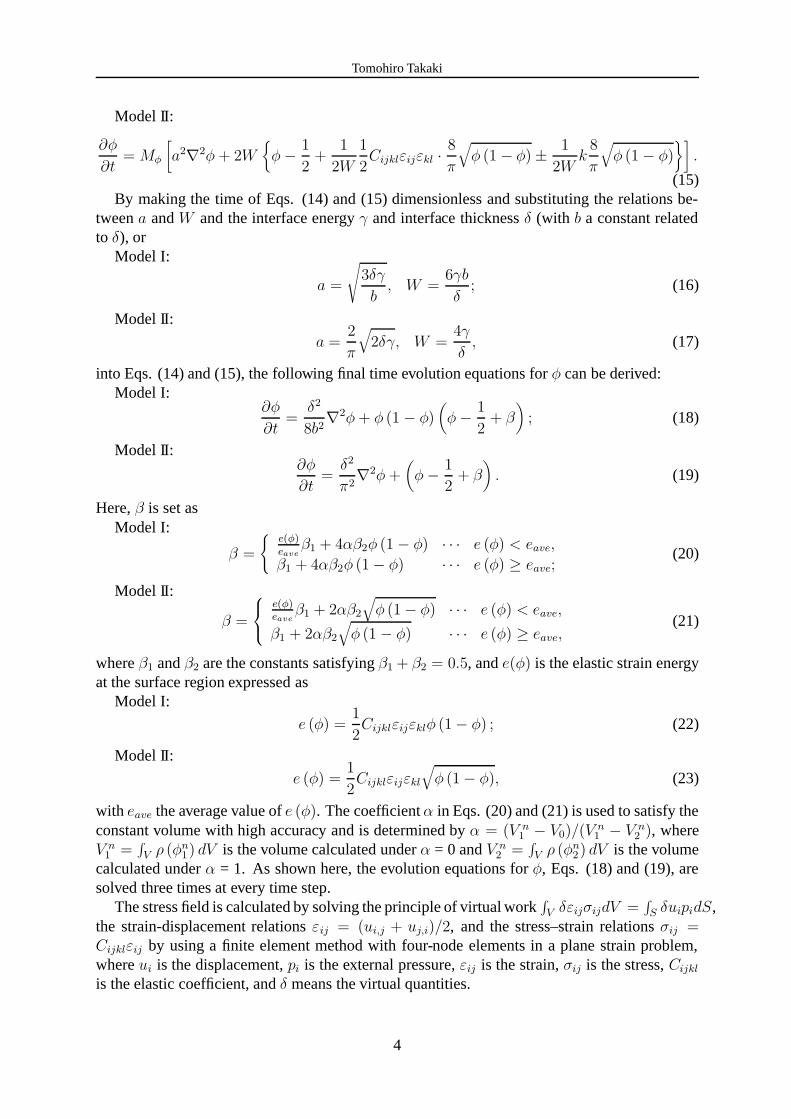
Stiffness maximization simulations of a cantilever using the two developed models are per-formed and the results are compared. Figure 2 shows the employed cantilever model with size400Δx×200Δx, where Δx is the square element size. The nodal displacements of the left sideare constrained in all directions and an external force is applied to the central node on the rightside.

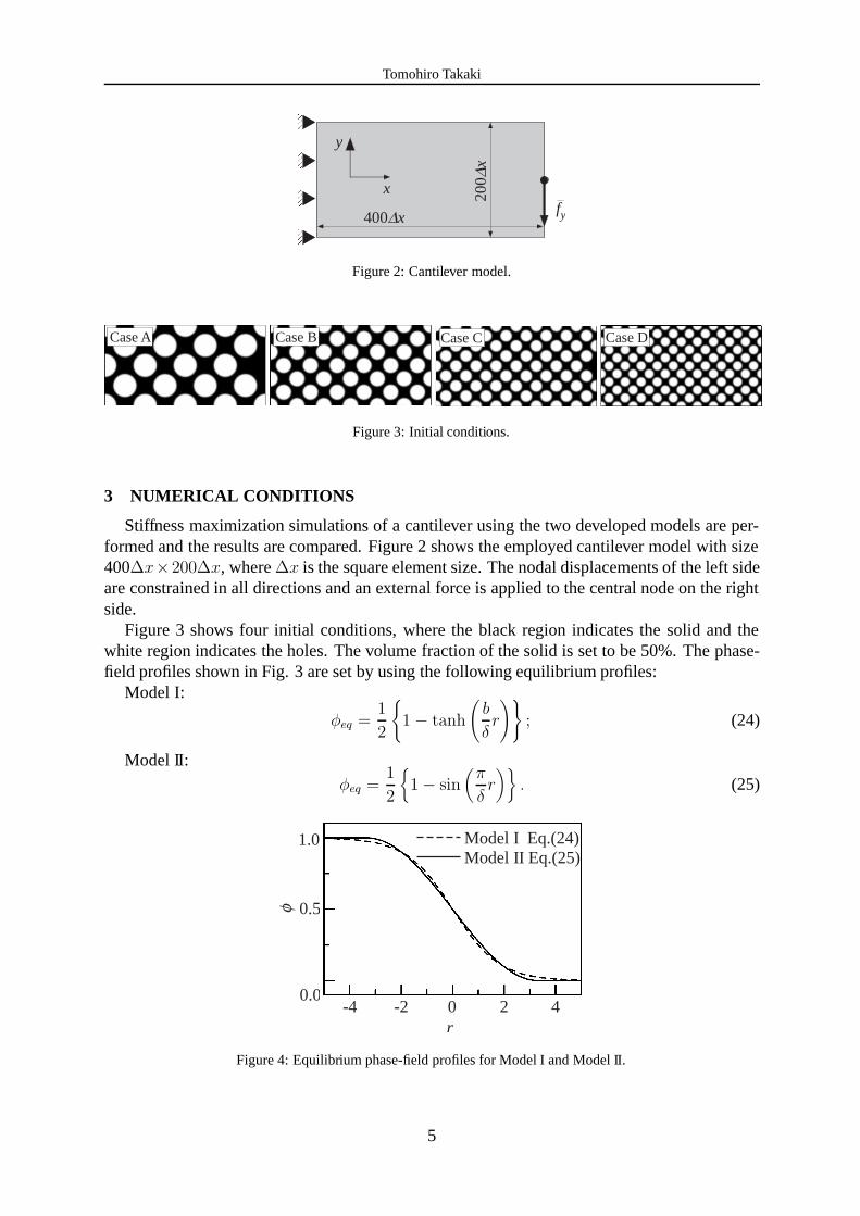
Figure 3 shows four initial conditions, where the black region indicates the solid and thewhite region indicates the holes. The volume fraction of the solid is set to be 50%. The phase-field profiles shown in Fig. 3 are set by using the following equilibrium profiles:

Model I:

φeq =1

2

{1 − tanh

(b

δr

)}; (24)

Model II:

φeq =1

2

{1 − sin

(π

δr)}

. (25)

0.0

1.0

0.5φ

-4 40r

2-2

Model I Eq.(24) Model II Eq.(25)

Figure 4: Equilibrium phase-field profiles for Model I and Model II.

5

Tomohiro Takaki

Figure 4 shows the phase-field profiles around the interface indicated by Eqs. (24) and (25).Here, δII = cδI = 1.682δI, δI = 4, and b = 2.2 are employed, where δI and δII are the interfacethickness δ for Model I and Model II, respectively. The relation c = 1.682 is derived by settingaI = aII or MφI = MφII.

Case A Case B Case C Case D

dI = 2Dx

dI = 3Dx

dI = 4Dx

dI = 5Dx

1.000

0.999

0.985

0.983

1.001

1.000

0.999

0.996

0.989

0.997

0.987

0.986

1.002

0.998

0.984

0.977

(a) Model I

dII = c2Dx

dII = c3Dx

dII = c4Dx

dII = c5Dx

Case A Case B Case C Case D

1.001

0.999

0.985

0.982

1.002

1.000

0.992

0.987

0.987

0.987

0.979

0.987

1.001

0.996

0.988

0.963

(b) Model II

Figure 5: Final morphologies.

4 NUMERICAL RESULTS

Figure 5 shows the final morphologies at 10000 steps for (a) Model I and (b) Model II.Here, the time increment Δt is set to 8b2(Δx)2/(5δ2) and π2(Δx)2/(5δ2) for Models I and II, respectively. The interface thicknesses δI for Model I are 2Δx, 3Δx, 4Δx, and 5Δx, and δII

6

Tomohiro Takaki

values for Model II are 3.364Δx, 5.046Δx, 6.728Δx, and 8.410Δx in order to keep the relationδII = 1.682δI. The numerical values indicated in Fig. 5 are the stiffness ratios for the conditionδI = 2Δx and Case A.

In Fig. 5, the effects of initial morphology on the final morphology are not absent but arerelatively small. There are one or two types of topologies with the same interface thickness, al-though there are a few exceptions. Therefore, it is concluded that the dependencies on the initialmorphology are relatively small. For the effects of interface thickness on the final morphology,it is observed that the stiffness increases with decreasing interface thickness. However, if theinterface thickness become smaller than 2Δx, the calculation become unstable. Therefore, thesuitable interface thickness is δ = 2Δx or 3Δx.

0 500 1000 1500

1.0

0.6

0.2

0.4

0

0.8

Step No.

Stif

fnes

s ra

tio

Model I Model II

Figure 6: Variations in stiffness ratio for the condition of δ = 2Δx and Case A.

100 step 200 step 300 step

400 step 500 step 10000 step

Figure 7: Morphological changes for Model I, with δ = 2Δx, for Case A.

Comparing Model I and Model II, we can see similar final morphologies. Figure 6 showsvariations in the stiffness ratio for the condition of δ = 2Δx and Case A. The stiffness is definedas the value where the applied force f̄ is divided by the displacement of the point. The ordinateof Fig. 6 is the ratio to the initial condition. It is confirmed that variations in the stiffness ratiofor both models are almost identical with monotonic increases. Figure 7 shows the variationsof morphology of Model I for the conditions of Fig. 6. At the beginning of the calculation, thecircular holes changed shape to squares in order to arrange the solid along the principal stressdirection. After that, the solid in the upper and lower regions around the applied concentrated

7

Tomohiro Takaki

force disappears. These morphological changes occur to increase the structure stiffness, asseen in Fig. 6. However, from Fig. 5(b), a few nonsymmetrical morphologies in the upperand lower regions can be observed in Model II. Therefore, it is concluded that a phase-fieldtopology optimization model with a double-obstacle function can be used to calculate almostthe same final morphologies as a model with a double-well function, although it sometimesexhibits unstable results.

5 CONCLUSIONS

A phase-field topology optimization model with a double-obstacle function was derived to-gether with a model with a double-well function. By performing two-dimensional topologyoptimization simulations for a cantilever subjected to a concentrated force, the fundamentalcharacteristics of the developed model were investigated. As a result, it was commonly con-cluded for both models that the effects of initial morphology on the final morphology are rel-atively small and higher stiffness values are obtained for thinner interfaces. Furthermore, thedeveloped model with a double-obstacle function can be used to calculate an almost similar finalmorphology with a similar stiffness as a model with a double-well function, although some finalnonsymmetrical shapes appear in upper and lower regions of the model with a double-obstaclefunction.

REFERENCES

[1] M. P. Bendsœ, O. Sigmund: Topology Optimization (2002), Springer.

[2] A. Takezawa, S. Nishiwaki, M. Kitamura: Shape and topology optimization based onthe phase field method and sensitivity analysis. Journal of Computational Physics, 229(2010), 2697–2718.

[3] T. Takaki: Development of phase-field topology optimization model and its fundamen-tal performance evaluations. Transactions of the Japan Society of Mechanical EngineersSeries A, 77 (2011), 1840–1850 (in Japanese).

[4] I. Steinbach, F. Pezzolla: A generalized field method for multiphase transformations usinginterface fields. Physica D, 134 (1999), 385–393.

8