A Method for Staffing Large Call Centers Based on Stochastic

Fluid Models

J. Michael Harrison∗

Stanford UniversityAssaf Zeevi

†

Columbia University

Submitted : September 2003 Revised: February 2004

To appear in Manufacturing & Service Operations Management

Abstract

We consider a call center model with m input flows and r pools of agents; the m-vector λ ofinstantaneous arrival rates is allowed to be time-dependent and to vary stochastically. Seekingto optimize the trade-off between personnel costs and abandonment penalties, we develop andillustrate a practical method for sizing the r agent pools. Using stochastic fluid models, thismethod reduces the staffing problem to a multi-dimensional newsvendor problem, which canbe solved numerically by a combination of linear programming and Monte Carlo simulation.Numerical examples are presented, and in all cases the pool sizes derived by means of theproposed method are very close to optimal.

Short Title: Staffing Large Call Centers

Keywords: Capacity sizing, call centers, fluid analysis, multi-dimensional newsvendor, non-stationarity.queueing, random environment, stochastic programming.

∗Graduate School of Business, e-mail: harrison michael@gsb.stanford.edu†Graduate School of Business, e-mail: assaf@gsb.columbia.edu

1

1 Introduction

From an operations research perspective, the two central problems of telephone call center man-

agement are (a) the assignment of agents to work schedules, which we call the staff scheduling

problem, and (b) the dynamic routing of calls to agents given system status, which we call the

dynamic routing problem. This paper is directly concerned with the first of those problems, and

because the two problems are inextricably linked, it is indirectly concerned with the second one as

well.

As usual in OR studies, we view a call center as a queueing system, frequently referring to

callers as “customers” and to call center agents as “servers.” The general model that we adopt

has m customer classes and r server pools. Server pool k consists of bk interchangeable agents

(k = 1, . . . , r) whose capabilities will be described shortly. Customers of the various classes arrive

randomly over time, and those who cannot be served immediately wait in a (possibly virtual)

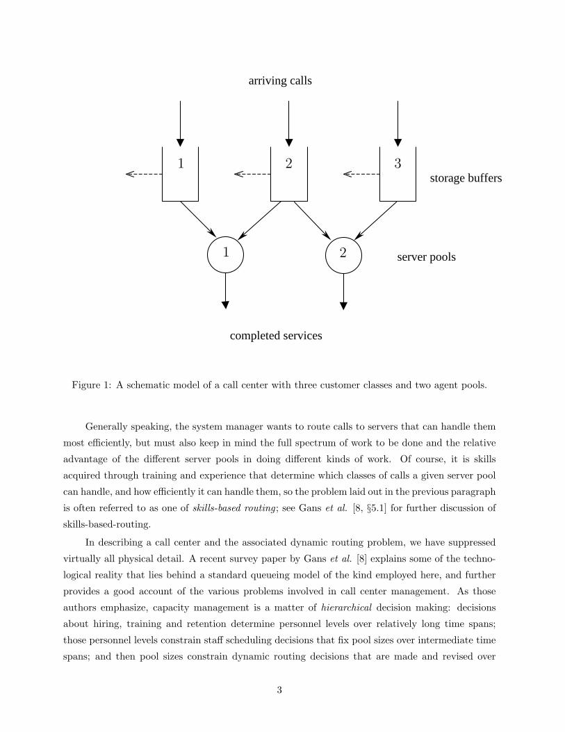
infinite-capacity buffer that is dedicated to their specific class. An example with m = 3 customer

classes and r = 2 server pools is portrayed schematically in Figure 1; buffers are represented by

open-ended rectangles and server pools by circles. An important assumption of our model is that

customers of any given class will abandon their calls if forced to wait too long before commencement

of service; abandoned calls are represented by the horizontal dotted arrows emanating from the

storage buffers in Figure 1. Our assumptions regarding speed of abandonment will be explained

later.

The servers in a given pool may be cross-trained to handle customers of several different

classes, and by the same token, there may be several pools able to handle a given customer class.

For the example portrayed in Figure 1, each server pool can handle two of the three customer

classes; customers of class 2 can be served by either pool, but each of the other two classes can be

served by just one pool. In general, we allow the service time distribution of a customer to depend

on both the customer’s class and on the pool from which the server comes.

The dynamic routing problem referred to earlier is the following. First, whenever a customer

arrives and there exist one or more idle servers who can handle that customer’s class, the system

manager must choose between routing the customer immediately to one of them versus putting

the customer into buffer storage for later disposition. If the customer is to be routed immediately,

there may be a further choice regarding the server pool to which it will be routed. Second, each

time a server completes the processing of a customer and there exist waiting customers of one or

more classes that the server can handle, the system manager must choose between routing one of

those customers to the server immediately versus idling the server in anticipation of future arrivals.

These resource allocation decisions are conditioned on system status information at the time of the

choice, including numbers of customers waiting in the various buffers and numbers of servers idle

in the various pools.

2

arriving calls

storage buffers

server pools completed services

1

1

2

2 3

Figure 1: A schematic model of a call center with three customer classes and two agent pools.

Generally speaking, the system manager wants to route calls to servers that can handle them

most efficiently, but must also keep in mind the full spectrum of work to be done and the relative

advantage of the different server pools in doing different kinds of work. Of course, it is skills

acquired through training and experience that determine which classes of calls a given server pool

can handle, and how efficiently it can handle them, so the problem laid out in the previous paragraph

is often referred to as one of skills-based routing ; see Gans et al. [8, §5.1] for further discussion of

skills-based-routing.

In describing a call center and the associated dynamic routing problem, we have suppressed

virtually all physical detail. A recent survey paper by Gans et al. [8] explains some of the techno-

logical reality that lies behind a standard queueing model of the kind employed here, and further

provides a good account of the various problems involved in call center management. As those

authors emphasize, capacity management is a matter of hierarchical decision making: decisions

about hiring, training and retention determine personnel levels over relatively long time spans;

those personnel levels constrain staff scheduling decisions that fix pool sizes over intermediate time

spans; and then pool sizes constrain dynamic routing decisions that are made and revised over

3

short time spans.

Ignoring the first or highest level of that hierarchy, we shall address the following, somewhat

stylized version of the second-level problem in the body of this paper, explaining afterward how the

analysis can be extended to recognize more of the fine structure that characterizes real-world staff

scheduling. First, the decision variables in our formulation are the pool sizes b1, . . . br identified

earlier, which we treat as continuous variables. The treatment of pool sizes as continuous variables

reflects our primary focus on large call centers; see section 3 for further discussion.

Second, in our formulation of the staff scheduling problem, a system manager must determine

in advance the capacity vector b = (b1, . . . , br) to be employed during a specified planning period;

by assumption, that decision cannot be revised as actual demand is observed during the period.

(In a typical application, a day would be broken into several such planning periods.) Third, we

express service-level concerns in our formulation by attaching a penalty of pi dollars to each class

i customer that abandons his or her call; as we shall explain later (see section 6), the formulation

can easily be extended to further incorporate a linear waiting cost for each customer class. Finally,

given the personnel cost ck associated with employing one server in pool k for the duration of

the planning period (k = 1, . . . , r), our objective is to minimize the sum of personnel costs plus

expected total abandonment cost.

The crucial task in addressing this problem is to estimate best achievable performance with a

given capacity vector b, by which we mean the smallest expected abandonment cost that can be

achieved over the course of the planning period with the specified capacity vector. Our proposed

method for call center staffing is based on a linear programming estimate of best achievable per-

formance, an estimate that appears crude but has nonetheless proved surprisingly accurate in a

realistic parameter regime (see section 3).

Roughly speaking, our method ignores all uncertainty and all variability in the call center

environment except for that associated with average arrival rates, or average demand rates. We

employ a very general model of call center demand in which the m-vector λ of average arrival

rates for the various customer classes (expressed in units like calls per minute) is both temporally

and stochastically variable; that is, we view λ itself as a stochastic process. As Gans et al. [8]

acknowledge in section 4.4 of their survey paper, such a view is realistic, although most published

papers on both call center staffing and dynamic routing treat average arrival rates as known and

constant over the relevant planning period. (Moreover, to the best of our knowledge, all commercial

software products that support those functions are based on similar modeling assumptions.)

To repeat, we take the view that temporal and stochastic variability of average demand rates,

over a time span that is appropriate for staff scheduling purposes, are not only significant but

actually dominant; we treat all other sources of variability as essentially negligible by comparison.

(To capture that perspective mathematically, we adopt a stochastic fluid model in which arrivals

4

and departures both appear as continuous fluid flows.)

The previous paragraphs suggest that our method for call center staffing stands in contrast

to other methods that have been proposed in the literature. That statement is somewhat decep-

tive, however, because there is no literature on staffing methods with multiple pools and multiple

customer classes, except for the fragmentary results reported in section 5 of Gans et al. [8]. The

correct statement is that when one specializes our method to the simple case of one customer class

and one server pool, which is essentially the only setting considered in the current literature, it is

clearly distinguished from earlier work. A striking virtue of our method is that it applies to the

general multi-class-and-multi-pool problem, which Gans et al. [8] characterize in section 5 of their

survey paper as far beyond the reach of current theory.

Existing modeling approaches and related work. As indicated above, studies of call

center staffing have focused on the case of a single pool of homogenous agents. Basic queueing

models, in particular, the Erlang-C formula for the M/M/N queueing model (see [8]), provide

the main mathematical analysis tool in that setting. A widely-used rule-of-thumb that emerges

from the Erlang-C formula is the square-root safety staffing rule, cf. Kolesar and Green [16], which

recommends a server pool size of the form N = R + β√

R, where R is the nominal incoming

load measured in Erlangs. This relationship apparently dates back to early work of Erlang in

1924, see [7] and Gans et al. [8, §4.1.1] for further discussion and references, and Halfin and

Whitt [11] for a more rigorous justification using diffusion limits. A recent asymptotic analysis

of the staffing problem in the context of the M/M/N single-class/single-pool call center model

was carried out by Borst et al. [4]. They refine the square-root rule by optimizing over β to

balance queueing and staffing costs. Garnett et al. [9] extend the square-root staffing principle

to account for abandonments, while Jennings et al. [15] adjust this formalism to account for

non-stationary demand using infinite-server approximations. All of these results pertain to the

single-class/single-pool Markovian queueing model. In the context of temporally varying demand,

heuristics such as pointwise stationary approximations (see [10]) are often used. Fluid limits, which

take a macroscopic view of the system dynamics, provide a more rigorous analysis framework for

non-stationary queueing systems; see [18] for a treatment of Markovian service networks which are

inspired by call center models, and [5] which studies a web-service system with transient overload

and uncertain demand using stochastic fluid models. Effects of uncertainty and non-stationarity

are discussed in [6], and [1] uses simulation and cutting plane methods to optimize costs subject to

service level constraints.

Planning periods and objective function. Two important elements of our problem for-

mulation deserve further emphasis. With regard to the critical notion of ”planning period,” we

implicitly assume that one or both of the following conditions prevail: (a) the staffing decision

for any given planning period must be finalized well before the period actually begins, so there is

5

significant uncertainty at the time of the decision about the average arrival rates that will apply;

(b) planning periods cannot be made so short (that is, staff levels cannot be changed so often)

that temporal variation in average arrival rates within a planning period is negligible. Thus, in

the typical situation that we envision, a call center will be either clearly overstaffed or clearly

understaffed most of the time, even with optimal decision making, because the system manager

lacks the ability to finely tune capacity in response to observed demand; one might say that our

modeling assumptions constitute a reduced-expectations view of system management. Based on

conversations with industry professionals, we believe this view is consistent with practical reality,

but we have no hard evidence to support that belief.

The system manager’s objective in our formulation is to minimize the sum of staffing costs and

expected abandonment penalties for the various customer classes. That is not the standard view of

optimal staffing in the call center industry. Call center managers are much more comfortable with

planning based on percentiles of the waiting time distribution. For example, a commonly stated

goal is to minimize staffing costs subject to the constraint that 80% of calls should be answered in 10

seconds or less; with two customer classes, it might be specified that 90% of class 1 customers wait

less than 10 seconds, and 80% of class 2 wait less than 20 seconds. At least on the surface, it is much

more difficult to minimize staffing costs subject to an array of such performance constraints than

to minimize the objective function that we propose. In our formulation, abandonment penalties

serve as surrogates for the system manager’s performance goals. Our hope and belief is that by

iteratively adjusting the abandonment penalties, one can eventually derive a policy that makes a

reasonable trade-off between staffing costs and customer service, and between service goals for the

different classes. To put this in another way, we proceed under the assumption that performance

goals can be adequately ”dualized” by a suitable choice of abandonment penalties.

The remainder of the paper. In section 2 we describe our method, emphasizing data

inputs and computational mechanics rather than model assumptions. Readers will find that our

specification of the method is less than fully detailed. In a sense, we reduce one problem to another,

without saying exactly how the latter is to be solved, but the missing elements can reasonably be

characterized as discretionary technical details. In section 3 we provide supporting logic for the

proposed method, including a description of the parameter regime in which we expect it to work

well. In the course of that discussion two mathematical conjectures regarding limit theory are

advanced in rough form, but we make no attempt to justify our method in a rigorous mathematical

sense, or even to specify with complete precision just what our model of a call center is.

Section 4 is devoted to the simple case with one customer class and one server pool, in order to

give readers a clearer understanding of our method’s essential character and to make connections

with existing literature. In section 5 we present a family of closely related numerical examples

that all have the following crucial and relatively rare property: there exists an obvious “dominant

6

strategy” for dynamic routing, and so one can use brute-force simulation to determine a nearly-

optimal staffing plan for each example, then compare its total cost against that achieved by our

method. (One cannot make such a comparison for an arbitrary example, because one does not

know the optimal dynamic routing policy given pool sizes.) In all cases considered, the vector

of pool sizes determined by our method is nearly optimal, and our seemingly crude estimate of

best achievable performance is very accurate as well. Section 6 contains some concluding remarks,

including refinements of our method (described in broad outline) to account for aspects of real-

world staff scheduling that are ignored in the body of the paper. The section also identifies several

obvious directions for further research.

2 Description of the Proposed Staffing Method

To describe server capabilities in our call center model, we shall use the previously established

notion of processing “activities” as in Harrison and Lopez [13]; see also Harrison [12] for a broader

discussion of this concept and its role in stochastic systems theory. There are a total of n pro-

cessing activities available to the system manager in our general call center model, each of which

corresponds to agents from one particular pool serving customers of one particular class. (Thus

the total number of activities is n = 4 for the system portrayed in Figure 1.) For each activity

j = 1, . . . , n we denote by i(j) the customer class being served, by k(j) the server pool involved,

and by µj the associated mean service rate (that is, the reciprocal of the mean of the associated

service time distribution).

Let R and A be an m × n matrix and an r × n matrix, respectively, defined as follows: for

each j = 1, . . . , n set Rij = µj if i = i(j) and Rij = 0 otherwise, and set Akj = 1 if k = k(j)

and Akj = 0 otherwise. Thus one interprets R as an input-output matrix, precisely as in Harrison

and Lopez [13]: its (i, j)th element specifies the average rate at which activity j removes class i

customers from the system. Also, A is a capacity consumption matrix as in [13]: its (k,j)th element

is 1 if activity j draws on the capacity of server pool k and is zero otherwise. In addition to the

matrices R and A, our method for call center staffing requires as data the vector p = (p1, . . . , pm)

of penalty rates, and the vector c = (c1, . . . , cr) of personnel costs (see section 1). The only other

input required is a probability distribution F on Rm+ that is associated with the demand process;

this will be explained in the paragraphs that follow.

In the following discussion of demand modeling, time t = 0 represents the start of the planning

period and time t = T is its end. For the sake of concreteness we shall speak initially in terms of a

doubly stochastic Poisson model of demand, which means the following. There is given a stochastic

process Λ = (Λ(t) : 0 ≤ t ≤ T ) taking values in Rm+ , and given that Λ(t) = λ = (λ1, . . . , λm), the

conditional distribution of arrivals in customer classes 1, . . . , m immediately after time t is that of

7

independent Poisson processes with average arrival rates λ1, . . . , λm respectively (0 ≤ t < T ). It is

the distribution of the stochastic process Λ with which we shall be concerned.

For each λ ∈ Rm+ and b ∈ R

r+ let us denote by π∗(λ, b) the optimal objective value of the

following linear program (LP): choose an n-vector x to

minimize π = p · (λ − Rx) (1)

subject to

Rx ≤ λ, Ax ≤ b, and x ≥ 0. (2)

This LP problem represents what might be called a local fluid version of the system manager’s

dynamic scheduling problem: attaching to λ and b the same meanings as before, one interprets x

as the number of servers dedicated to activity j in the immediate future (j = 1, . . . , n); Rx is the

vector of output rates from the various customer classes generated by that program of activities,

and Ax is a vector whose components show how many servers in the various pools are occupied

(as opposed to idle). Additional interpretation and motivation of the LP problem (1) – (2) will be

provided in the next section.

The initial specification of our proposed method for call center staffing, to be simplified shortly,

is the following: choose the capacity vector b to

minimize c · b + E

{∫ T

0

π∗(Λ(t), b) dt

}

, (3)

where E{·} denotes expected value over possible realizations of the stochastic process Λ. Again, the

reasoning that supports this recommendation is delayed until the next section. However, because

the initial term c · b in the objective function (3) represents the total personnel cost associated with

capacity vector b, readers may have already inferred that the second term in (3) is the LP-based

estimate of best achievable performance that was referred to in section 1. This is indeed the case.

To recast the optimization problem (3) in a standard form, let us define the cumulative

distribution function

F (λ) :=1

T

∫ T

0

P{Λ(t) ≤ λ} dt for λ ∈ Rm+ . (4)

One interprets F (λ) as the expected fraction of time (within the planning period under study)

during which Λ(·) ≤ λ. It is now an elementary exercise to prove that (3) is equivalent to the

following (if Λ is a finite-valued process, this is just a matter of definition, and then one can use a

monotone, finite-valued approximations to establish the general equivalence):

minimize c · b + T

∫

Rm

+

π∗(λ, b) dF (λ) =: φ(b). (5)

In the literature of stochastic programming, this kind of problem is called a two-stage LP with

recourse: at the first stage a system manager chooses the capacity vector b and incurs cost c ·b; then

8

a random demand vector λ with distribution F is observed, and given that observation, the system

manager chooses at the second stage a vector x of activity levels that solve the linear programming

problem (1)-(2). This particular kind of two-stage problem embodied in (5) is sometimes called a

multi-dimensional newsvendor problem; see, e.g., the recent survey by Van Mieghem [22].

With regard to numerical solution techniques, two distinct computational approaches appear in

the literature of stochastic programming, cf. [3]. First, various exact methods can be used when the

distribution F concentrates its mass on a relatively small number of points, and second, approximate

methods based on Monte Carlo simulation can be used in the general case. To elaborate on the

latter approach in our particular context, observe that π∗(λ, ·) is convex for each fixed λ (this is a

standard result in linear programming theory), which directly implies the following.

Proposition 1 The minimand φ in (5) is a convex function on Rr+.

Given that our problem is one of convex optimization, the gradient-descent method can be

used for its numerical solution, with Monte Carlo simulation providing the means to estimate ∇φ(b)

for each trial value of b; see Shapiro [21] for a recent survey of such methods. This approach will

be applied to a small-scale example in section 5, but it looks to be practical for problems of the

size encountered in real call center applications.

As stated earlier, the central feature of our call center model is the assumption of a random

demand environment, meaning that the vector of average or expected arrival rates is itself viewed

as a stochastic process Λ. We have thus far spoken in terms of doubly stochastic Poisson arrivals,

but the Poisson assumption has not actually been used. The method that we propose for call center

staffing does not depend on the fine stochastic structure of customer arrival processes given Λ (it

would make no difference, for example, if arrival streams were correlated given Λ), because we treat

routine stochastic variability given Λ as insignificant compared to variations in Λ itself.

Thus far nothing has been said about how to estimate the distribution F , which summarizes

all that is relevant about demand variability for purposes of our method, from operational data

in a given call center environment. That could be the subject of a paper by itself, and we cannot

claim to have even thought through the various alternatives systematically as yet. However, one

relatively simple and widely applicable approach will be described in section 6.

3 Supporting Logic

To motivate the staffing method described in section 2, we need to justify the second term in (3)

as a reasonable estimate of best achievable performance for a given capacity vector b. First, more

must be said about the abandonment mechanism in our call center model. We assume there exist

abandonment rates γ1, . . . , γm > 0 such that, when there are qi customers waiting for service in

9

the class i buffer at time t, the expected number of class i abandonments in the interval (t, t + h)

is approximately (γiqi)h for small h > 0 (i = 1, . . . , m). This may be viewed as a consequence of

the following more detailed assumption, which is standard in call center modeling, see Garnett et

al. [9], Harrison and Zeevi [14], and Gans et al. [8]: there is associated with each class i caller an

exponentially distributed random variable τ that has mean 1/γi, and the customer will abandon

the call when his or her waiting time (exclusive of service time) reaches a total of τ time units.

To justify the performance estimate embodied in (3), let us first consider a scenario where

the vector λ of average arrival rates is known and constant (that is, not time-varying) and the

time horizon for the dynamic routing problem is infinite. Assuming that the arrival rates λi are

large enough to make large pool sizes (on the order of tens, say) economically desirable, the law

of large numbers provides a rough justification for the following fluid model of dynamic routing,

cf. Maglaras [17]. First, the total number of class i customers at any given time t is modeled as

a continuous variable zi(t) ≥ 0, and the state of the system at time t is represented by the vector

z(t) = [z1(t), . . . , zm(t)]. Second, having observed z(t), the system manager chooses a control vector

x(t) = [x1(t), . . . , xn(t)] that satisfies the constraints

Ax(t) ≤ b, Bx(t) ≤ z(t), and x(t) ≥ 0, (6)

where B is an m × n matrix with Bij = 1 if i = i(j) and Bij = 0 otherwise. One interprets xj(t)

as the number of servers devoted to activity j at time t; recall that k(j) is the pool to which such

servers belong, and i(j) is the class of customers that they serve when engaged in activity j. The

first set of constraints in (6) requires that, for each pool k = 1, . . . , r, the total number of servers

from pool k that are assigned to various activities is no larger than the number bk that exist. The

second set of constraints requires that, for each customer class i = 1, . . . , m, the total number of

servers assigned to processing class i customers is no larger than the number of such customers

present in the system.

Let us define the m-vector q(t) = z(t) – Bx (t), so that qi(t) represents the number of class

i customers waiting at time t, excluding the ones being served, as above. Then yi(t) := γiqi(t)

is the instantaneous departure rate from buffer i at time t due to abandonment. That is, setting

Γ = diag(γ1, . . . , γm), we define an m-vector

y(t) = Γ[z(t) − Bx(t)], t ≥ 0, (7)

and then the dynamic evolution of our fluid control problem is governed by the following system

of ordinary differential equations:

z(t) = λ − Rx(t) − y(t), t ≥ 0. (8)

Also, the instantaneous cost rate at time t is

π(t) :=m

∑

i=1

piγiqi(t) = p · y(t), t ≥ 0. (9)

10

To avoid technical distractions, we shall restrict attention from the outset to controls x(·) for

which

x := limT→∞

1

T

∫ T

0

x(t) dt (10)

exists. Because all the abandonment rates γi are strictly positive by assumption, it is easy to prove

that z(·) is bounded. Thus, integrating (10) over the interval [0, T ], dividing both sides by T and

letting T → ∞, one has

1

T

∫ T

0

y(t) dt → (λ − Rx) =: y as T → ∞, (11)

and the long-run average cost rate π that we are striving to minimize in our fluid control problem

is given by

π := p · y = p · (λ − Rx). (12)

Let π∗(λ, b) be the optimal objective value of the linear programming problem (1)–(2) as in

section 2. Because y(t) ≥ 0 for all t ≥ 0, and hence y ≥ 0, we have from (11) that Rx ≤ λ, and

(6) implies Ax ≤ b and x ≥ 0. That is, x is a feasible solution for the LP problem (1)–(2). Thus,

under any admissible control x(·) one has

π ≥ π∗(λ, b). (13)

Fixing an optimal solution x∗ of the LP problem (1)–(2), it is easy to construct from x∗

an admissible control that achieves the lower bound in (13). In verbal terms, one simple way to

accomplish this is the following. First, for each j= 1, . . . , n we permanently dedicate x∗j servers from

pool k(j) to activity j, which means that those servers are permanently dedicated to processing

class i(j) customers. Any servers who are not permanently dedicated in that first step remain

permanently idle. Second, at each time t we match or assign as many customers as possible to

servers that have been dedicated to that class, and it is immaterial just how that matching is done.

To express this mathematically, let us focus specifically on customer class 1. Let the n activities

be numbered in such a way that activities j = 1, . . . , ℓ are the only ones that have i(j) = 1 and

x∗j > 0. That is, activities 1, . . . , ℓ are precisely the ones to which servers are permanently dedicated

for the processing of class 1 customers. Let

fj(z1) := [z1 − (x∗1 + · · · + x∗

j−1)]+ ∧ x∗

j for j = 1, . . . , l and z1 ≥ 0, (14)

with fj(·) = 0 for all j ∈ {l + 1, . . . , n} such that i(j) = 1. Now we take

xj(t) = fj(z1(t)), t ≥ 0, (15)

for all j ∈ {1, . . . , n} such that i(j) = 1. In words, this means the following: of the z1(t) class 1

customers who are present at time t, we first allocate as many as possible to the x∗1 servers from pool

11

k(1) who are dedicated to activity 1, then allocate as many as possible to the x∗2 servers from pool

k(2) who are dedicated to activity 2, and so on through the allocation of class 1 customers to servers

from pool k(ℓ) who are dedicated to activity ℓ; if not all class 1 customers have been allocated to

a server at that point, the remainder wait in buffer storage. The assignment of customers first

to servers from pool k(1), . . ., and last to those from pool k(ℓ) is arbitrary; what matters for the

argument below is that we assign or match as many customers as possible to dedicated servers.

It is easy to verify that, under the control strategy just described, the general relationship (8)

specializes to give

z1(t) = g1(z1(t)), t ≥ 0, (16)

where g1(·) is piecewise linear and strictly decreasing on [0,∞) with the following properties:

g1(0) = λ1 > 0, (17)

g1(z∗1) = 0, where z∗1 = (x∗

1 + · · · + x∗l ) +

1

γ1

(λ − Rx∗)1, (18)

g1(z1) = −γ1(z1 − z∗1) for z1 ≥ z∗1 . (19)

It follows that z1(t) → z∗1 as t → ∞; in fact, z1(t) ↑ z∗1 if z1(0) ≤ z∗1 and z1(t) ↓ z∗1 if z1(0) ≥ z∗1 .

For each j = 1, . . . , ℓ we have fj(z∗1) = x∗

j , implying that xj(t) → x∗j as t → ∞, and thus xj = x∗

j .

Repeating the construction and argument in identical fashion for other customer classes, one

obtains xj = x∗j for all j = 1, . . . , n, and hence π = (λ − Rx∗) = π∗(λ, b) by (11) and (12). In

words, π∗(λ, b) represents the best achievable performance (that is, the smallest achievable long

run average cost rate) in our fluid approximation to the steady-state dynamic scheduling problem

with λ known and constant.

To further develop our justification for the objective function in (3), consider a scenario where

sample paths of the stochastic process Λ(·) are constant over one-hour intervals within the planning

period, but the value of Λ(·) that will obtain over each such interval is unknown at the time when

pool sizes must be decided. Let us further suppose that the average service rates µ1, . . . , µn and

average abandonment rates γ1, . . . , γm are all around 60 per hour, which means that the average

service time for each customer class is something close to one minute, and so is the average time

that a customer will wait before abandoning a call. In this situation our dynamic routing problem

evolves on a much faster time scale than does the vector of average demand rates: given the value

λ taken on by Λ(·) at the beginning of a one-hour interval, and assuming as before that total flow

rates are large enough to justify a fluid approximation, one is led to approximate the minimum

average cost rate achievable over the interval by the steady-state performance estimate π∗(λ, b).

Generalizing that piecewise-constant demand scenario in the obvious way, we assume that

average service rates µj and average abandonment rates γi are large relative to the time scale on

which demand changes occur. Thus one can reasonably employ a steady-state approximation for

the lowest cost rate that is achievable in the dynamic scheduling problem given the value of Λ(·)

12

that pertains at any given time. Further assuming that call volumes are adequate to justify a fluid

approximation for the problem of steady-state performance estimation given that Λ(·) = λ, one

arrives at (3).

There are two standard means of bolstering user confidence in approximations like ours. The

first is to analyze numerical examples; that course will be followed in sections 4 and 5 below.

Second, one may strive to prove that the proposed approximation is in some sense “asymptotically

optimal” in a limiting parameter regime. We shall not attempt such an analysis here, but it may be

worthwhile to at least articulate in a concrete manner the form of such a result. (For further details

and a rigorous derivation see Bassamboo et al. [2].) Starting with a single call center model of the

kind described in section 1, let us denote by b∗ an optimal solution of the minimization problem

(3), and let f : R+ 7→ R+ be any non-decreasing and super-linear function (that is, κ−1f(κ) → ∞as κ → ∞). Now consider a cognate model defined as follows. First, all service and abandonment

processes are accelerated by a uniform factor of κ > 1. Second, the original cost vector c is replaced

by κc, which means that the effective cost of capacity, expressed in terms of potential services per

time unit, remains constant. Finally, all arrival processes are accelerated by a uniform factor of

f(κ), meaning that Λ(·) is replaced by f(κ)Λ(·).It is easy to verify that in the cognate model, the vector of pool sizes recommended by our

method is κ−1f(κ)b∗. That is, the original capacity choice b∗ is scaled up by a factor of f(κ) to

reflect the acceleration of arrival processes, but then scaled down by a factor of κ to reflect the

acceleration of service processes. In [2] it will be shown that this choice is asymptotically optimal

in the following sense: both the expected total cost (over the planning period being analyzed) with

our proposed vector of pool sizes, and the minimum expected total cost achievable with any choice,

are asymptotic to f(κ)φ(b∗) as κ → ∞, where φ(·) is defined for the original model via (8) and (9).

This statement corresponds to what is called fluid-scale asymptotic optimality in the literature of

applied probability, cf. Maglaras [17] and Meyn [19].

4 A Special Case: Homogeneous Customers and Agents

Let us consider now the special case with a single customer class (m = 1) and a single agent pool

(r = 1). There is then a single processing activity (n = 1), and we denote by µ > 0 the associated

average service rate. Recalling that T denotes the length of planning horizon, we assume that

c < Tpµ. (20)

That is, the cost to employ one server for the length of the planning period is less than the expected

total abandonment cost that the server can prevent if continuously busy. (If this inequality did not

hold, the optimal pool size would be b∗ = 0.)

13

In the current context one can solve the LP problem (1)–(2) by inspection: the optimal solution

is x∗ = λ ∧ (bµ), and the optimal objective value is

π∗(λ, b) = p(λ − x∗) = p(λ − bµ)+. (21)

Of course, F is now a probability distribution on [0,∞), and using (21) one can express the objective

function φ in our optimization problem (5) as

φ(b) = cb + Tp

∫ ∞

0

(λ − bµ)+dF (λ) = cb + Tp

∫ ∞

bµ

(1 − F (λ)) dλ . (22)

Assuming for simplicity that F is a continuous (atomless) distribution, one can differentiate (22)

with respect to b and set the derivative equal to zero to obtain the following characterization of the

optimal pool size b∗:

F (b∗µ) = 1 − c

Tpµ. (23)

Minimization of the objective function (22) is the classical newsvendor problem of operations re-

search: if one could know the demand λ before choosing a capacity b, the best choice would be

b = λ/µ, but lacking such clairvoyance, one must choose b so as to optimize the trade-off between

(linear) overage costs and (linear) underage costs; the choice which optimizes that trade-off is the

critical fractile solution (23).

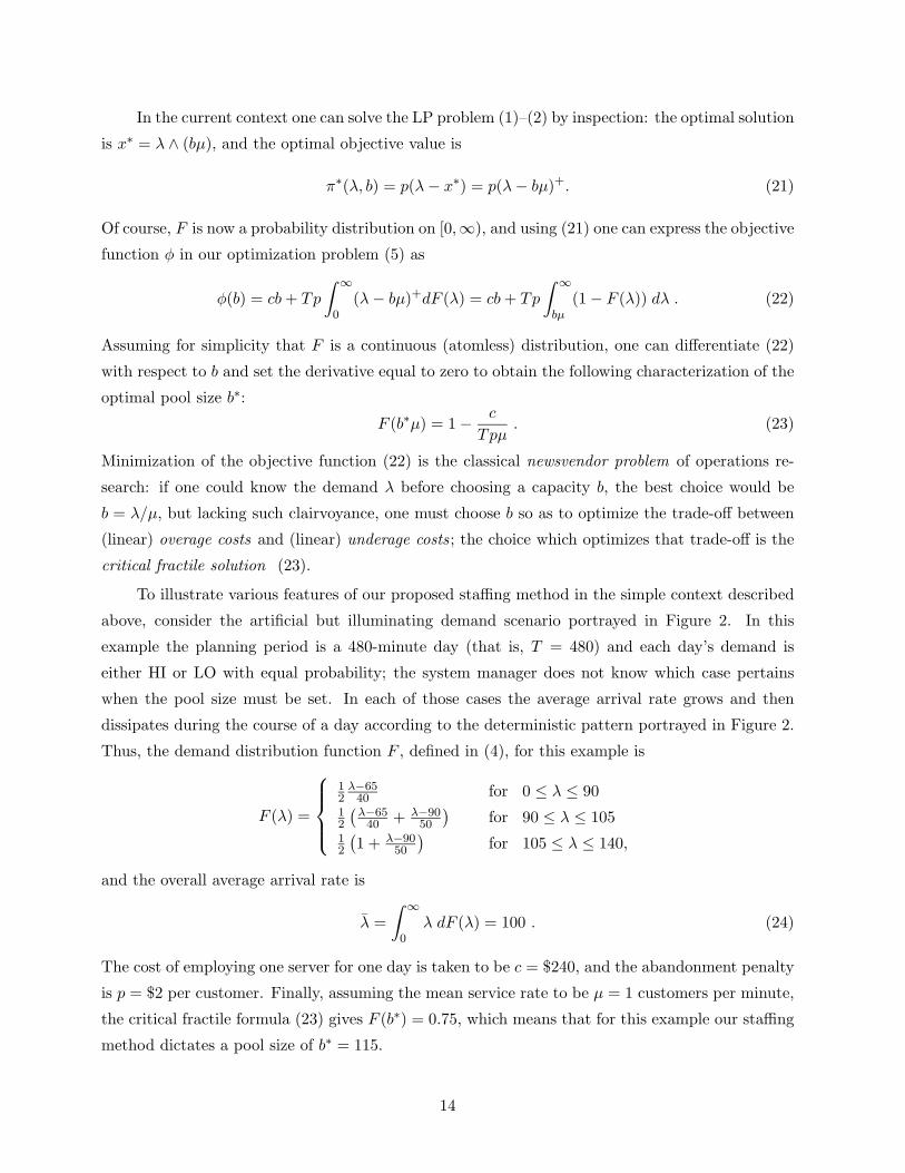
To illustrate various features of our proposed staffing method in the simple context described

above, consider the artificial but illuminating demand scenario portrayed in Figure 2. In this

example the planning period is a 480-minute day (that is, T = 480) and each day’s demand is

either HI or LO with equal probability; the system manager does not know which case pertains

when the pool size must be set. In each of those cases the average arrival rate grows and then

dissipates during the course of a day according to the deterministic pattern portrayed in Figure 2.

Thus, the demand distribution function F , defined in (4), for this example is

F (λ) =

1

2

λ−65

40for 0 ≤ λ ≤ 90

1

2

(

λ−65

40+ λ−90

50

)

for 90 ≤ λ ≤ 1051

2

(

1 + λ−90

50

)

for 105 ≤ λ ≤ 140,

and the overall average arrival rate is

λ =

∫ ∞

0

λ dF (λ) = 100 . (24)

The cost of employing one server for one day is taken to be c = $240, and the abandonment penalty

is p = $2 per customer. Finally, assuming the mean service rate to be µ = 1 customers per minute,

the critical fractile formula (23) gives F (b∗) = 0.75, which means that for this example our staffing

method dictates a pool size of b∗ = 115.

14

0 60 120 180 240 300 360 420 48060

70

80

90

100

110

120

130

140

150

160

Time (minutes)

Ave

rage

dem

and

rate

(cust

omer

sper

min

ute

)

HI

LO

Figure 2: Illustrative demand pattern.

To simplify analysis of the example, we make the following assumptions. First, both service

times and inter-abandonment times are exponentially distributed, with parameters µ = 1 and

γ = 0.5, respectively. Thus the average service time is one minute, and the average time that a

customer will wait in the queue before abandoning is two minutes. Second, arrivals occur according

to a non-homogeneous Poisson process whose intensity parameter Λ(·) evolves according to the

pattern portrayed in Figure 2. Of course, there are no dynamic routing decisions to be made in this

simple system: servers process customers on a first-in-first-out basis, say, and there is no motivation

to interrupt a service once it has begun, even if one assumes that is possible.

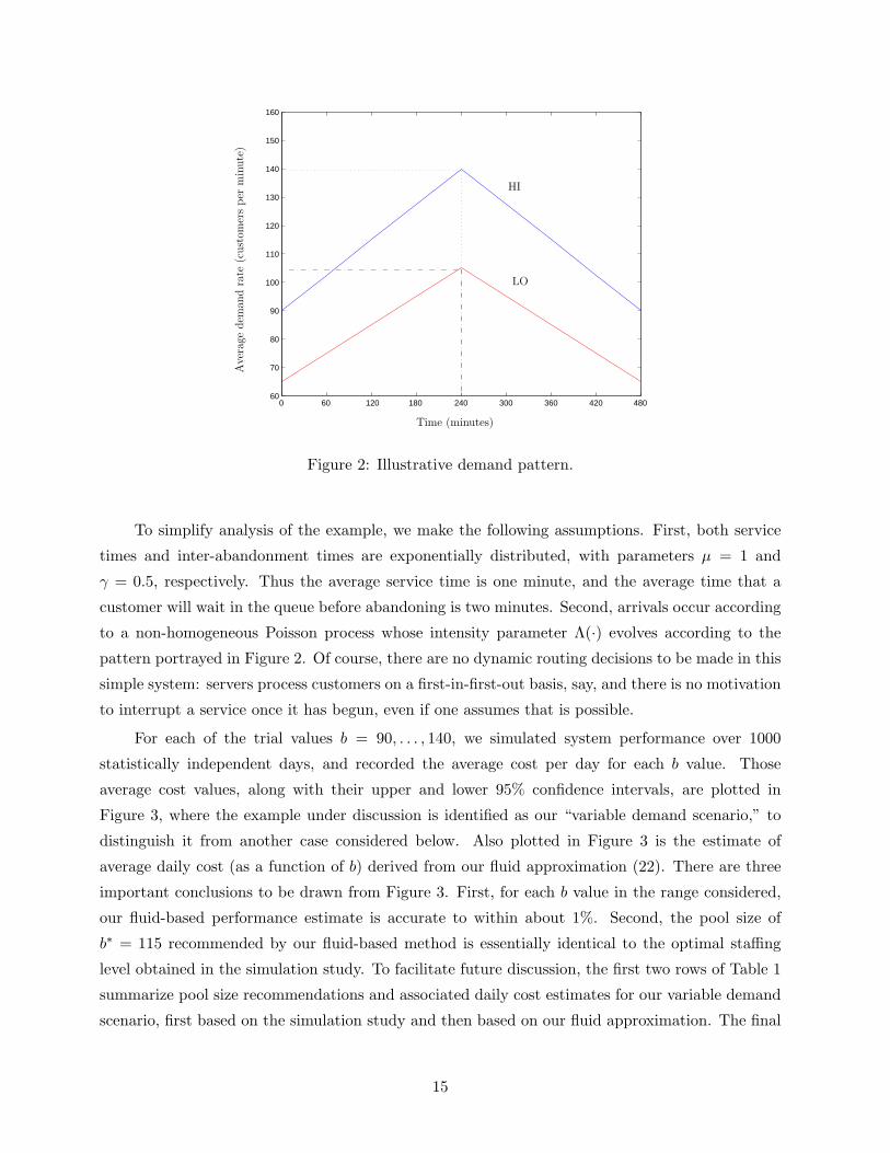
For each of the trial values b = 90, . . . , 140, we simulated system performance over 1000

statistically independent days, and recorded the average cost per day for each b value. Those

average cost values, along with their upper and lower 95% confidence intervals, are plotted in

Figure 3, where the example under discussion is identified as our “variable demand scenario,” to

distinguish it from another case considered below. Also plotted in Figure 3 is the estimate of

average daily cost (as a function of b) derived from our fluid approximation (22). There are three

important conclusions to be drawn from Figure 3. First, for each b value in the range considered,

our fluid-based performance estimate is accurate to within about 1%. Second, the pool size of

b∗ = 115 recommended by our fluid-based method is essentially identical to the optimal staffing

level obtained in the simulation study. To facilitate future discussion, the first two rows of Table 1

summarize pool size recommendations and associated daily cost estimates for our variable demand

scenario, first based on the simulation study and then based on our fluid approximation. The final

15

conclusion to be drawn from Figure 3 is that system performance is relatively insensitive to the

pool size b in the neighborhood of the minimizer, according to both our simulation results and

the fluid approximation. Finally, statistical variability in the simulation decreases as the pool size

increases, as seen in the “shrinking” confidence intervals in the figure, since more customers are

served upon arrival and queueing effects decrease.

90 95 100 105 110 115 120 125 130 135 1403

3.1

3.2

3.3

3.4

3.5

3.6

3.7

Number of servers (b)

Tot

alav

erag

edai

lyco

st($

10K

)

simulation

fluid approximation

upper 95% confidence interval

lower 95% confidence interval

Figure 3: Total average daily cost as a function of the number of servers: variable demand scenario.

Due to high variability in the simulation results, the plot depicts the 95% confidence interval (dotted

lines).

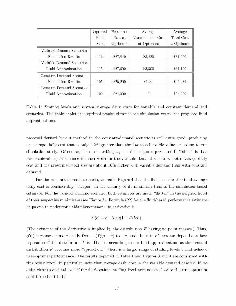
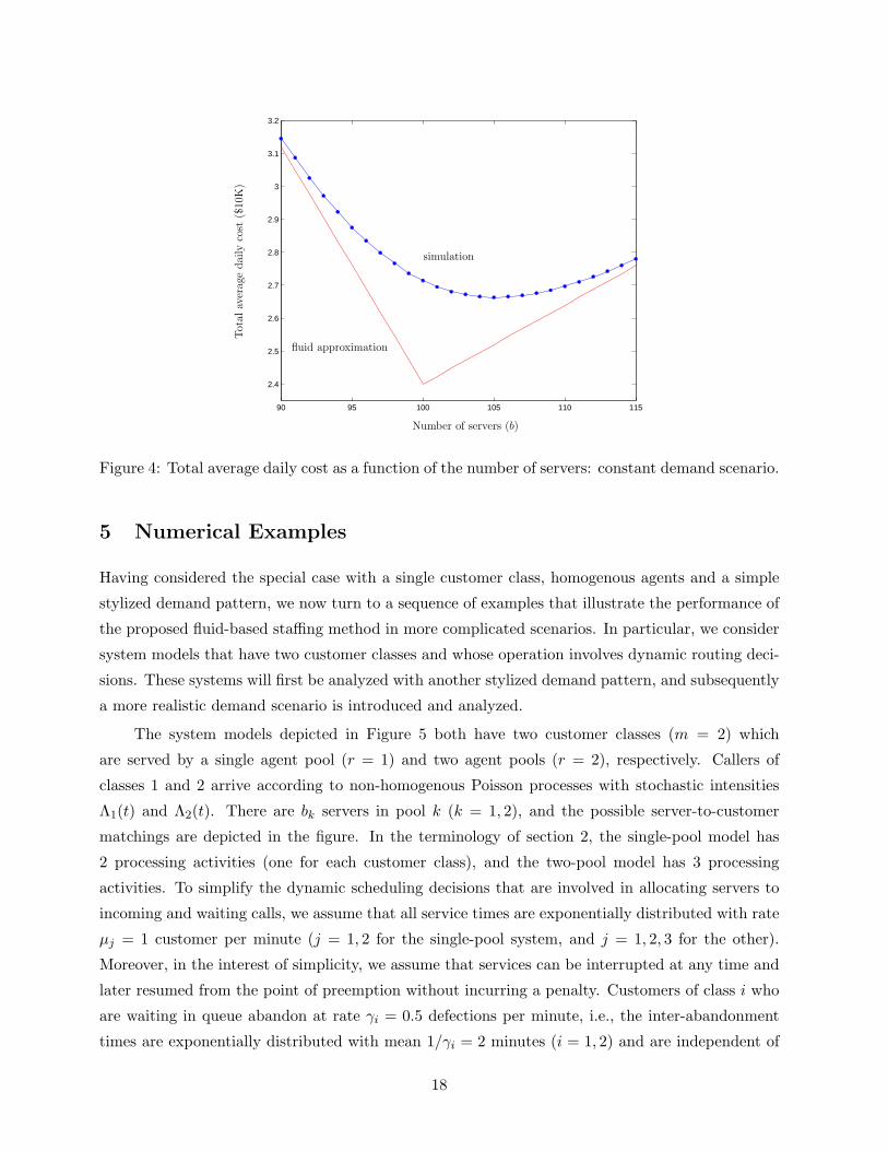
It is interesting to contrast the example just discussed with a “constant demand scenario”

where Λ(·) is identically equal to the overall average value, λ = 100 that was identified earlier in

(24). Figure 4 presents both the fluid-based performance estimate derived from (22) for that case,

and the corresponding simulation results, again based on a sample of 1000 independent days for

each b value. (In this case the 95% confidence intervals are so close to the simulation estimates

of average daily cost, relative to the scale of the graph, that we have just omitted them.) The

third and fourth rows of Table 1 summarize pool size recommendations and associated daily cost

estimates for the constant demand scenario, first based on the simulation study and then based

on our fluid approximation. Of course, the staffing level recommended by our method is trivially

b∗ = 100.

For choices of b close to the optimal value, our fluid-based approximation of average daily

cost is almost 10% lower in the constant-demand scenario than our simulation estimate. (Recall

that the error is about 1% in the variable-demand scenario.) On the other hand, the naıve staffing

16

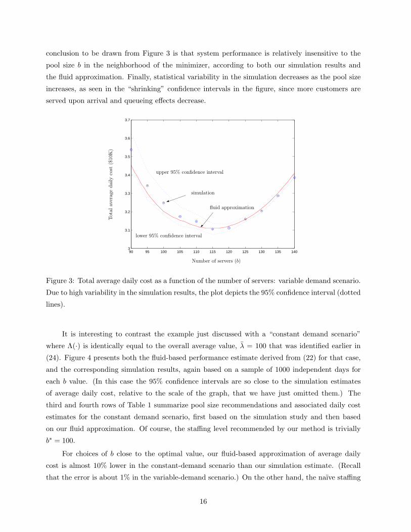
Optimal Personnel Average Average

Pool Cost at Abandonment Cost Total Cost

Size Optimum at Optimum at Optimum

Variable Demand Scenario:

Simulation Results 116 $27,840 $3,220 $31,060

Variable Demand Scenario:

Fluid Approximation 115 $27,600 $3,500 $31,100

Constant Demand Scenario:

Simulation Results 105 $25,200 $1439 $26,639

Constant Demand Scenario:

Fluid Approximation 100 $24,000 0 $24,000

Table 1: Staffing levels and system average daily costs for variable and constant demand and

scenarios. The table depicts the optimal results obtained via simulation versus the proposed fluid

approximations.

proposal derived by our method in the constant-demand scenario is still quite good, producing

an average daily cost that is only 1-2% greater than the lowest achievable value according to our

simulation study. Of course, the most striking aspect of the figures presented in Table 1 is that

best achievable performance is much worse in the variable demand scenario: both average daily

cost and the prescribed pool size are about 10% higher with variable demand than with constant

demand.

For the constant-demand scenario, we see in Figure 4 that the fluid-based estimate of average

daily cost is considerably “steeper” in the vicinity of its minimizer than is the simulation-based

estimate. For the variable-demand scenario, both estimates are much “flatter” in the neighborhood

of their respective minimizers (see Figure 3). Formula (22) for the fluid-based performance estimate

helps one to understand this phenomenon: its derivative is

φ′(b) = c − Tpµ(1 − F (bµ)).

(The existence of this derivative is implied by the distribution F having no point masses.) Thus,

φ′(·) increases monotonically from −(Tpµ − c) to +c, and the rate of increase depends on how

“spread out” the distribution F is. That is, according to our fluid approximation, as the demand

distribution F becomes more “spread out,” there is a larger range of staffing levels b that achieve

near-optimal performance. The results depicted in Table 1 and Figures 3 and 4 are consistent with

this observation. In particular, note that average daily cost in the variable demand case would be

quite close to optimal even if the fluid-optimal staffing level were not as close to the true optimum

as it turned out to be.

17

90 95 100 105 110 115

2.4

2.5

2.6

2.7

2.8

2.9

3

3.1

3.2

Number of servers (b)

Tot

alav

erag

edai

lyco

st($

10K

)

simulation

fluid approximation

Figure 4: Total average daily cost as a function of the number of servers: constant demand scenario.

5 Numerical Examples

Having considered the special case with a single customer class, homogenous agents and a simple

stylized demand pattern, we now turn to a sequence of examples that illustrate the performance of

the proposed fluid-based staffing method in more complicated scenarios. In particular, we consider

system models that have two customer classes and whose operation involves dynamic routing deci-

sions. These systems will first be analyzed with another stylized demand pattern, and subsequently

a more realistic demand scenario is introduced and analyzed.

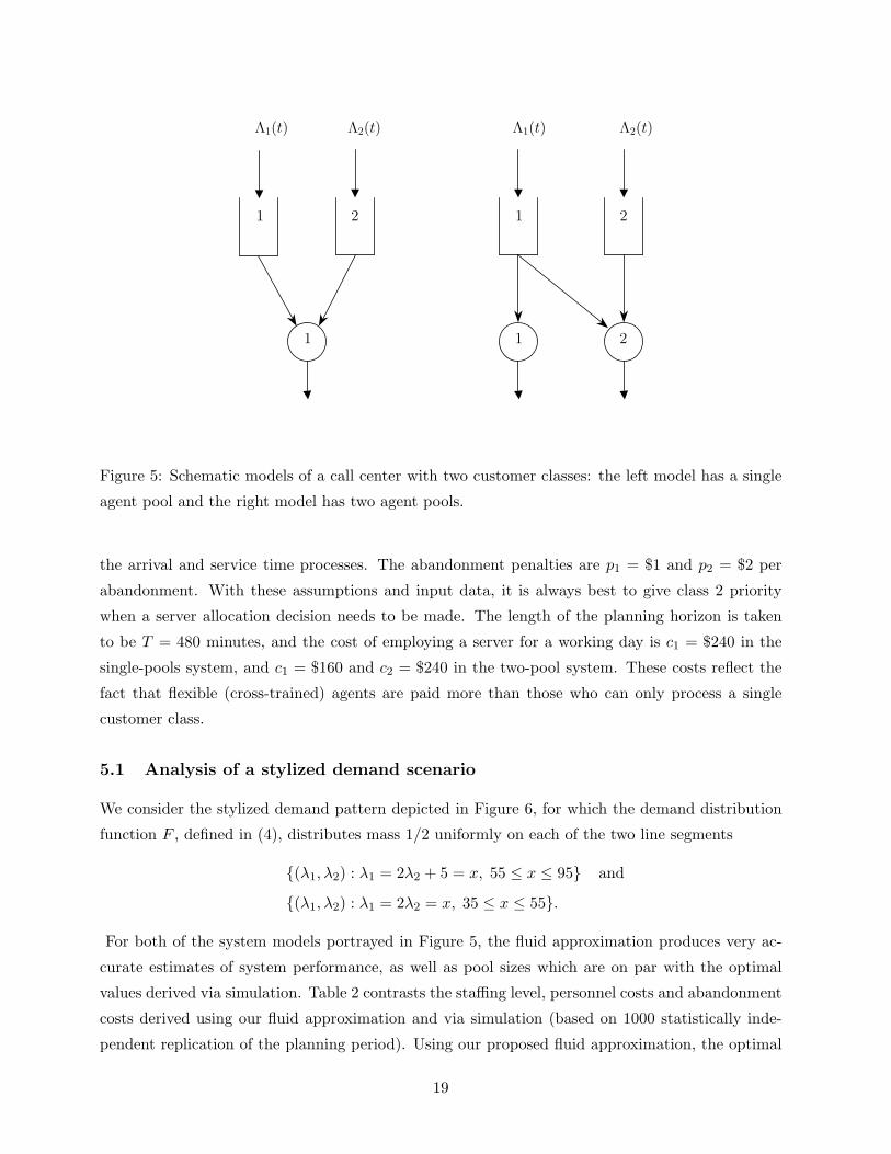
The system models depicted in Figure 5 both have two customer classes (m = 2) which

are served by a single agent pool (r = 1) and two agent pools (r = 2), respectively. Callers of

classes 1 and 2 arrive according to non-homogenous Poisson processes with stochastic intensities

Λ1(t) and Λ2(t). There are bk servers in pool k (k = 1, 2), and the possible server-to-customer

matchings are depicted in the figure. In the terminology of section 2, the single-pool model has

2 processing activities (one for each customer class), and the two-pool model has 3 processing

activities. To simplify the dynamic scheduling decisions that are involved in allocating servers to

incoming and waiting calls, we assume that all service times are exponentially distributed with rate

µj = 1 customer per minute (j = 1, 2 for the single-pool system, and j = 1, 2, 3 for the other).

Moreover, in the interest of simplicity, we assume that services can be interrupted at any time and

later resumed from the point of preemption without incurring a penalty. Customers of class i who

are waiting in queue abandon at rate γi = 0.5 defections per minute, i.e., the inter-abandonment

times are exponentially distributed with mean 1/γi = 2 minutes (i = 1, 2) and are independent of

18

Λ1(t)Λ1(t) Λ2(t)Λ2(t)

11

11

2

22

Figure 5: Schematic models of a call center with two customer classes: the left model has a single

agent pool and the right model has two agent pools.

the arrival and service time processes. The abandonment penalties are p1 = $1 and p2 = $2 per

abandonment. With these assumptions and input data, it is always best to give class 2 priority

when a server allocation decision needs to be made. The length of the planning horizon is taken

to be T = 480 minutes, and the cost of employing a server for a working day is c1 = $240 in the

single-pools system, and c1 = $160 and c2 = $240 in the two-pool system. These costs reflect the

fact that flexible (cross-trained) agents are paid more than those who can only process a single

customer class.

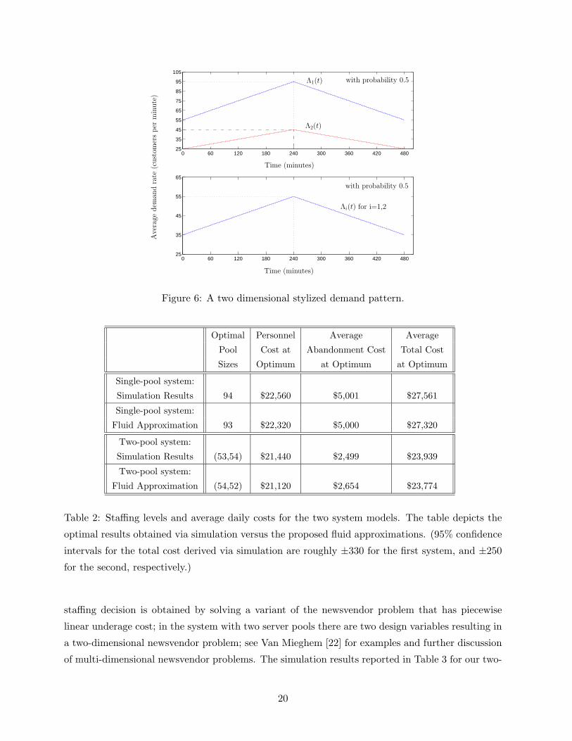
5.1 Analysis of a stylized demand scenario

We consider the stylized demand pattern depicted in Figure 6, for which the demand distribution

function F , defined in (4), distributes mass 1/2 uniformly on each of the two line segments

{(λ1, λ2) : λ1 = 2λ2 + 5 = x, 55 ≤ x ≤ 95} and

{(λ1, λ2) : λ1 = 2λ2 = x, 35 ≤ x ≤ 55}.

For both of the system models portrayed in Figure 5, the fluid approximation produces very ac-

curate estimates of system performance, as well as pool sizes which are on par with the optimal

values derived via simulation. Table 2 contrasts the staffing level, personnel costs and abandonment

costs derived using our fluid approximation and via simulation (based on 1000 statistically inde-

pendent replication of the planning period). Using our proposed fluid approximation, the optimal

19

0 60 120 180 240 300 360 420 48025

35

45

55

65

75

85

95

105

0 60 120 180 240 300 360 420 48025

35

45

55

65

Time (minutes)

Time (minutes)

Ave

rage

dem

and

rate

(cust

omer

sper

min

ute

)

Λ1(t)

Λ2(t)

Λi(t) for i=1,2

with probability 0.5

with probability 0.5

Figure 6: A two dimensional stylized demand pattern.

Optimal Personnel Average Average

Pool Cost at Abandonment Cost Total Cost

Sizes Optimum at Optimum at Optimum

Single-pool system:

Simulation Results 94 $22,560 $5,001 $27,561

Single-pool system:

Fluid Approximation 93 $22,320 $5,000 $27,320

Two-pool system:

Simulation Results (53,54) $21,440 $2,499 $23,939

Two-pool system:

Fluid Approximation (54,52) $21,120 $2,654 $23,774

Table 2: Staffing levels and average daily costs for the two system models. The table depicts the

optimal results obtained via simulation versus the proposed fluid approximations. (95% confidence

intervals for the total cost derived via simulation are roughly ±330 for the first system, and ±250

for the second, respectively.)

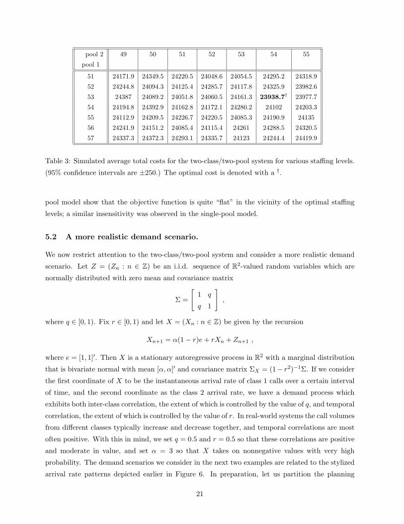
staffing decision is obtained by solving a variant of the newsvendor problem that has piecewise

linear underage cost; in the system with two server pools there are two design variables resulting in

a two-dimensional newsvendor problem; see Van Mieghem [22] for examples and further discussion

of multi-dimensional newsvendor problems. The simulation results reported in Table 3 for our two-

20

pool 2 49 50 51 52 53 54 55

pool 1

51 24171.9 24349.5 24220.5 24048.6 24054.5 24295.2 24318.9

52 24244.8 24094.3 24125.4 24285.7 24117.8 24325.9 23982.6

53 24387 24089.2 24051.8 24060.5 24161.3 23938.7† 23977.7

54 24194.8 24392.9 24162.8 24172.1 24280.2 24102 24203.3

55 24112.9 24209.5 24226.7 24220.5 24085.3 24190.9 24135

56 24241.9 24151.2 24085.4 24115.4 24261 24288.5 24320.5

57 24337.3 24372.3 24293.1 24335.7 24123 24244.4 24419.9

Table 3: Simulated average total costs for the two-class/two-pool system for various staffing levels.

(95% confidence intervals are ±250.) The optimal cost is denoted with a †.

pool model show that the objective function is quite “flat” in the vicinity of the optimal staffing

levels; a similar insensitivity was observed in the single-pool model.

5.2 A more realistic demand scenario.

We now restrict attention to the two-class/two-pool system and consider a more realistic demand

scenario. Let Z = (Zn : n ∈ Z) be an i.i.d. sequence of R2-valued random variables which are

normally distributed with zero mean and covariance matrix

Σ =

[

1 q

q 1

]

,

where q ∈ [0, 1). Fix r ∈ [0, 1) and let X = (Xn : n ∈ Z) be given by the recursion

Xn+1 = α(1 − r)e + rXn + Zn+1 ,

where e = [1, 1]′. Then X is a stationary autoregressive process in R2 with a marginal distribution

that is bivariate normal with mean [α, α]′ and covariance matrix ΣX = (1− r2)−1Σ. If we consider

the first coordinate of X to be the instantaneous arrival rate of class 1 calls over a certain interval

of time, and the second coordinate as the class 2 arrival rate, we have a demand process which

exhibits both inter-class correlation, the extent of which is controlled by the value of q, and temporal

correlation, the extent of which is controlled by the value of r. In real-world systems the call volumes

from different classes typically increase and decrease together, and temporal correlations are most

often positive. With this in mind, we set q = 0.5 and r = 0.5 so that these correlations are positive

and moderate in value, and set α = 3 so that X takes on nonnegative values with very high

probability. The demand scenarios we consider in the next two examples are related to the stylized

arrival rate patterns depicted earlier in Figure 6. In preparation, let us partition the planning

21

period (recall that its length is T = 480 minutes) into 18 sub-intervals of length ∆ = T/18 minutes,

and denote by ai(j) the expected average arrival rate for class i customers over the jth subinterval

when using the stylized demand model portrayed in Figure 6 (i = 1, 2 and j = 1, . . . , 18). Also, let

ai denote the expected average arrival rate for class i customers over the entire planning period in

the same demand model.

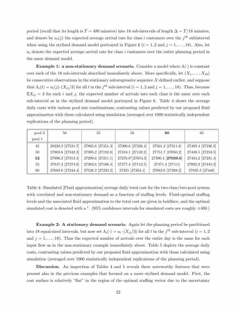
Example 1: a non-stationary demand scenario. Consider a model where Λ(·) is constant

over each of the 18 sub-intervals described immediately above. More specifically, let (X1, . . . , X18)

be consecutive observations in the stationary autoregressive sequence X defined earlier, and suppose

that Λi(t) = ai(j)·(Xij/3) for all t in the jth sub-interval (i = 1, 2 and j = 1, . . . , 18). Thus, because

EXij = 3 for each i and j, the expected number of arrivals into each class is the same over each

sub-interval as in the stylized demand model portrayed in Figure 6. Table 4 shows the average

daily costs with various pool size combinations, contrasting values predicted by our proposed fluid

approximation with those calculated using simulation (averaged over 1000 statistically independent

replications of the planning period).

pool 2 50 55 58 60 65

pool 1

45 28220.2 [27531.7] 27865.8 [27451.3] 27300.6 [27226.4] 27501.2 [27311.8] 27493.4 [27236.3]

50 27903.6 [27342.3] 27395.2 [27182.8] 27316.1 [27132.2] 27751.7 [27050.2] 27438.5 [27253.5]

52 27996.3 [27313.4] 27299.6 [27211.1] 27276.8†[27054.3] 27390.4 [27039.6] 27434.2 [27231.4]

55 27847.3 [27274.8] 27362.6 [27166.4] 27577.4 [27112.5] 27471.4 [27111] 27602.3 [27445.3]

60 27683.8 [27244.4] 27526.2 [27223.2] 27355 [27264.1] 27683.6 [27288.2] 27835.5 [27446]

Table 4: Simulated [Fluid approximation] average daily total cost for the two-class/two-pool system

with correlated and non-stationary demand as a function of staffing levels. Fluid-optimal staffing

levels and the associated fluid approximation to the total cost are given in boldface, and the optimal

simulated cost is denoted with a †. (95% confidence intervals for simulated costs are roughly ±400.)

Example 2: A stationary demand scenario. Again let the planning period be partitioned

into 18 equal-sized intervals, but now set Λi(·) = ai · (Xij/3) for all t in the jth sub-interval (i = 1, 2

and j = 1, . . . , 18). Thus the expected number of arrivals over the entire day is the same for each

input flow as in the non-stationary example immediately above. Table 5 depicts the average daily

costs, contrasting values predicted by our proposed fluid approximation with those calculated using

simulation (averaged over 1000 statistically independent replications of the planning period).

Discussion. An inspection of Tables 4 and 5 reveals three noteworthy features that were

present also in the previous examples that focused on a more stylized demand model. First, the

cost surface is relatively “flat” in the region of the optimal staffing vector due to the uncertainty

22

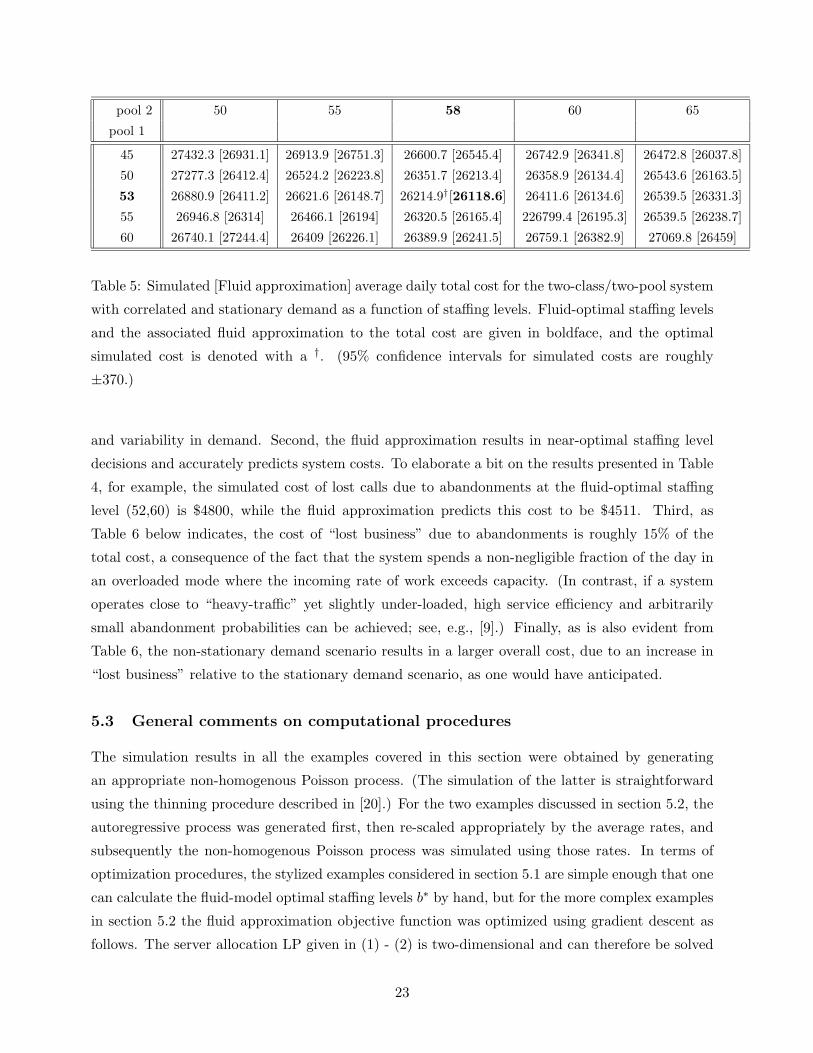
pool 2 50 55 58 60 65

pool 1

45 27432.3 [26931.1] 26913.9 [26751.3] 26600.7 [26545.4] 26742.9 [26341.8] 26472.8 [26037.8]

50 27277.3 [26412.4] 26524.2 [26223.8] 26351.7 [26213.4] 26358.9 [26134.4] 26543.6 [26163.5]

53 26880.9 [26411.2] 26621.6 [26148.7] 26214.9†[26118.6] 26411.6 [26134.6] 26539.5 [26331.3]

55 26946.8 [26314] 26466.1 [26194] 26320.5 [26165.4] 226799.4 [26195.3] 26539.5 [26238.7]

60 26740.1 [27244.4] 26409 [26226.1] 26389.9 [26241.5] 26759.1 [26382.9] 27069.8 [26459]

Table 5: Simulated [Fluid approximation] average daily total cost for the two-class/two-pool system

with correlated and stationary demand as a function of staffing levels. Fluid-optimal staffing levels

and the associated fluid approximation to the total cost are given in boldface, and the optimal

simulated cost is denoted with a †. (95% confidence intervals for simulated costs are roughly

±370.)

and variability in demand. Second, the fluid approximation results in near-optimal staffing level

decisions and accurately predicts system costs. To elaborate a bit on the results presented in Table

4, for example, the simulated cost of lost calls due to abandonments at the fluid-optimal staffing

level (52,60) is $4800, while the fluid approximation predicts this cost to be $4511. Third, as

Table 6 below indicates, the cost of “lost business” due to abandonments is roughly 15% of the

total cost, a consequence of the fact that the system spends a non-negligible fraction of the day in

an overloaded mode where the incoming rate of work exceeds capacity. (In contrast, if a system

operates close to “heavy-traffic” yet slightly under-loaded, high service efficiency and arbitrarily

small abandonment probabilities can be achieved; see, e.g., [9].) Finally, as is also evident from

Table 6, the non-stationary demand scenario results in a larger overall cost, due to an increase in

“lost business” relative to the stationary demand scenario, as one would have anticipated.

5.3 General comments on computational procedures

The simulation results in all the examples covered in this section were obtained by generating

an appropriate non-homogenous Poisson process. (The simulation of the latter is straightforward

using the thinning procedure described in [20].) For the two examples discussed in section 5.2, the

autoregressive process was generated first, then re-scaled appropriately by the average rates, and

subsequently the non-homogenous Poisson process was simulated using those rates. In terms of

optimization procedures, the stylized examples considered in section 5.1 are simple enough that one

can calculate the fluid-model optimal staffing levels b∗ by hand, but for the more complex examples

in section 5.2 the fluid approximation objective function was optimized using gradient descent as

follows. The server allocation LP given in (1) - (2) is two-dimensional and can therefore be solved

23

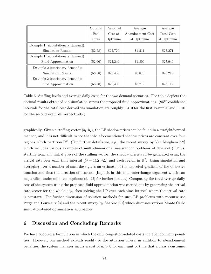
Optimal Personnel Average Average

Pool Cost at Abandonment Cost Total Cost

Sizes Optimum at Optimum at Optimum

Example 1 (non-stationary demand):

Simulation Results (52,58) $22,720 $4,511 $27,271

Example 1 (non-stationary demand):

Fluid Approximation (52,60) $22,240 $4,800 $27,040

Example 2 (stationary demand):

Simulation Results (53,58) $22,400 $3,815 $26,215

Example 2 (stationary demand):

Fluid Approximation (53,58) $22,400 $3,719 $26,119

Table 6: Staffing levels and average daily costs for the two demand scenarios. The table depicts the

optimal results obtained via simulation versus the proposed fluid approximations. (95% confidence

intervals for the total cost derived via simulation are roughly ±410 for the first example, and ±370

for the second example, respectively.)

graphically. Given a staffing vector (b1, b2), the LP shadow prices can be found in a straightforward

manner, and it is not difficult to see that the aforementioned shadow prices are constant over four

regions which partition R2. (For further details see, e.g., the recent survey by Van Mieghem [22]

which includes various examples of multi-dimensional newsvendor problems of this sort.) Thus,

starting from any initial guess of the staffing vector, the shadow prices can be generated using the

arrival rate over each time interval [(j − 1)∆, j∆) and each region in R2. Using simulation and

averaging over a number of such days gives an estimate of the expected gradient of the objective

function and thus the direction of descent. (Implicit in this is an interchange argument which can

be justified under mild assumptions; cf. [22] for further details.) Computing the total average daily

cost of the system using the proposed fluid approximation was carried out by generating the arrival

rate vector for the whole day, then solving the LP over each time interval where the arrival rate

is constant. For further discussion of solution methods for such LP problems with recourse see

Birge and Louveaux [3] and the recent survey by Shapiro [21] which discusses various Monte Carlo

simulation-based optimization approaches.

6 Discussion and Concluding Remarks

We have adopted a formulation in which the only congestion-related costs are abandonment penal-

ties. However, our method extends readily to the situation where, in addition to abandonment

penalties, the system manager incurs a cost of hi > 0 for each unit of time that a class i customer

24

spends waiting in the queue. (The term “linear holding cost” is commonly used to describe this

added model element.) By modifying appropriately the supporting logic described in section 2,

readers can verify that one arrives at the same staffing algorithm as before, except that the aban-

donment penalty pi that appears in the objective function (1) of our linear program is replaced by

pi + hi/γi (i = 1, . . . , m) in the case with linear holding costs.

In this paper, we have taken as given the basic system configuration, including the number

of server pools, the number of customer classes, the possible matchings of the latter to the former,

and the average service rates embodied in the input-output matrix R. We have developed a

fluid approximation that allows one to estimate best achievable system performance with a given

vector of pool sizes, and used that estimate to optimize pool sizes given the system configuration.

However, one can obviously extend this analytical method to evaluate and contrast competing

design configurations that propose different processing activities and agent pool structures. For

example, one can compare the two-class/two-pool system model depicted in Figure 5 with an

alternative that has two dedicated agent pools, each serving only a single designated class. In this

manner, it is possible to characterize the value of incorporating cross-trained agents into a given

system, as well as determine the extent to which such cross-training is necessary to achieve target

operating costs.

At least in principle, our method can be modified to take into account the workforce manage-

ment considerations described by Gans et al. in section 3.2 of their paper [8]. When one considers

the added structure that captures shift schedules, etc., one confronts a large set of discrete staffing

alternatives, rather than the continuum of choices assumed here. It is then possible to use our

proposed stochastic fluid approximation to estimate costs under each of those discrete alternatives.

Of course, this would require linking our performance evaluation method to an appropriate discrete

optimization technique. (For an example where simulation is used for purposes of performance

evaluation in conjunction with an integer program that is used to set staffing levels see Epelman

et al. [1].)

To apply our method in a given real-world context, the main task is to estimate the demand

distribution F defined by (4). A reasonable procedure for doing this, which accords well with

the estimation methods commonly used in call center practice, is the following. First, divide the

planing period into L intervals or “time buckets” of fixed length ∆, treating the process Λ as

piecewise constant over such intervals. (In practice it is common to take ∆ = one-half hour.) For

each realization of the arrival process over the planning period, and each time bucket ℓ = 1, . . . , L,

one can calculate an m-vector ξℓ of average arrival rates by taking the total number of arrivals in

each class i and dividing by ∆, and then ξ := (ξ1, . . . , ξL) describes one realization of the process

Λ. The empirical distribution of the finite sequence ξ, compiled from repeated observations of the

arrival process over the complete planning period, then provides the estimate of F for purposes of

25

our method. That is, drawing at random from the distribution F amounts to choosing at random

among the observed realizations of ξ, and then choosing at random a time bucket ℓ ∈ {1, . . . , L}.Obviously, the staffing method that we have proposed is only valid if one can devise a dynamic

routing policy whose performance with regard to expected abandonment costs approaches the LP-

based estimate of best achievable performance embodied in (3). In the interest of brevity we have

not attempted a systematic discussion of dynamic routing in this paper. However, a promising

general approach to dynamic routing is embodied in the “supporting logic” described in section 3.

Roughly speaking, the idea is to solve the linear programming problem (1)-(2) in real time, based

on a current estimate of the arrival rate vector λ, then allocate servers to customer classes over a

moderate time span based on the solution obtained, repeating this procedure at the end of that

time span. The asymptotic optimality of such an approach (in the parameter regime identified in

section 3), as well as variants of this basic idea that seem promising for practical implementation,

are the subject of Bassamboo et al. [2].

In this paper we have only emphasized uncertainty about the call center’s demand environ-

ment. In a similar fashion, call center managers are typically uncertain about actual capacity (in

the sense of average potential processing rates) given their staffing choices, due to factors such as

absenteeism, heterogeniety among agents who nominally belong to the same skill category, learning

effects, and a host of other factors. That is, call center managers are uncertain about their own

internal capabilities, quite apart from the statistical variation in service times. It seems plausible

that our method of accounting for large-scale demand uncertainty could be extended or modified

to account for uncertainty regarding internal capabilities, but no serious effort has been expended

in that direction to date.

Acknowledgements. The authors wish to thank Achal Bassamboo for his expert research as-

sistance with the simulation studies, and Andy Carr for sharing his knowledge and insights on

call center management. Also, the paper has benefitted substantially from the suggestions of two

anonymous referees.

References

[1] J. Atlason, M.A. Epelman, and S.G. Henderson. Call center staffing with simulation and

cutting plane methods. Ann. of Oper. Res., 2003. To appear.

[2] A. Bassamboo, J.M. Harrison, and A. Zeevi. Dynamic routing in large call centers: Asymptotic

analysis of an LP-based method. 2004. Working paper, Columbia University and Stanford

University.

26

[3] J.R. Birge and F. Louveaux. An introduction to stochastic programming. Springer Series in

Operations Research. Spinger, 1997.

[4] S. Borst, A. Mandelbaum, and M. Reiman. Dimensioning large call centers. Oper. Res., 2004.

To appear.

[5] J. Changa, H. Ayhan, J.G. Dai, and C.H. Xia. Dynamic scheduling of a multiclass fluid model

with transient overload. 2003. Working paper, Georgia Tech.

[6] B.P.K. Chen and S.G. Henderson. Two issues in setting call center staffing levels. Ann. of

Oper. Res., 108:175–192, 2001.

[7] A.K. Erlang. On the rational determination of the number of circuits. In H.L. Halstrom

E. Brockmeyer and A. Jensen, editors, The life and works of A.K. Erlang. The Copenhagen

Telephone Company, Copenhagen, 1948.

[8] N. Gans, G. Koole, and A. Mandelbaum. Telephone call centers: Tutorial, review, and research

prospects. Manufacturing & Service Operations Management, 5:79–141, 2003.

[9] O. Garnett, A. Mandelbaum, and M. Reiman. Designing a call center with impatient cus-

tomers. Manufacturing & Service Operations Management, 4:208–227, 2002.

[10] L.V. Green and P.J. Kolesar. The pointwise stationary approximation for queues with non-

stationary arrivals. Manag. Sci., 37:84–97, 1991.

[11] S. Halfin and W. Whitt. Heavy-traffic limits for queues with many exponential servers. Oper.

Res., 29:567–588, 1981.

[12] J.M. Harrison. Stochastic networks and activity analysis. In Y. Suhov, editor, Analytic methods

in Applied Probability, In memory of Fridrih Karpelevich. AMS, Providence, RI, 2002.

[13] J.M. Harrison and M.J. Lopez. Heavy traffic resourse pooling in parallel- server systems.

Queueing Systems, 33:339–368, 1999.

[14] J.M. Harrison and A. Zeevi. Dynamic scheduling of a multi-class queue in the Halfin-Whitt

heavy traffic regime. Oper. Res., 2004. To appear.

[15] O. Jennings, A. Mandelbaum, W. Massey, and W. Whitt. Server staffing to meet time-varying

demand. Manag. Sci., 42:1383–1394, 1996.

[16] P.J. Kolesar and L.V. Green. Insights on service system design from a normal approximation

to Erlang’s delay formula. Prod. Oper. Mgmt., 7:282–293, 1998.

27

[17] C. Maglaras. Discrete-review policies for scheduling stochastic networks: Trajectory tracking

and fluid-scale asymptotic optimality. Ann. Appl. Prob., 10:897–929, 2000.

[18] A. Mandelbaum, W. Massey, and M. Reiman. Strong approximations for Markovian service

networks. Queueing Systems, 30:149–201, 1998.

[19] S.P. Meyn. The policy improvement algorithm for M arkov decision processes with general

state space. IEEE Trans. Aut. Control, 42:1663–1680, 1997.

[20] S. Ross. Simulation. Academic Press, 1997.

[21] A. Shapiro. Stochastic programming by Monte Carlo simulation methods. In A. Ruszczyn-

ski and A. Shapiro, editors, Stochastic Programming, volume 10 of Handbooks in Operations

Research and Management Science. Elsevier North Holland, 2003.

[22] J.A. Van Mieghem. Capacity management, investment and hedging: Review and recent de-

velopments. Manufacturing & Service Operations Management, 5:269–302, 2003.

28