Stochastic Simulation: Lecture 7

Prof. Mike Giles

Oxford University Mathematical Institute

SDE Path Simulation

In these 2 lectures we are interested in SDEs of the form

dSt = a(St , t) dt + b(St , t) dWt

in which the multi-dimensional Brownian motion Wt hascovariance Σ.

The standard assumptions on the drift and diffusion functions are:

I Lipschitz in space:

‖a(x , t)−a(y , t)‖ ≤ La‖x−y‖, ‖b(x , t)−b(y , t)‖ ≤ Lb‖x−y‖,

I Holder in time:

‖a(x , s)− a(x , t)‖ ≤ La(1 + ‖x‖) |s−t|1/2,

‖b(x , s)− b(x , t)‖ ≤ Lb(1 + ‖x‖) |s−t|1/2

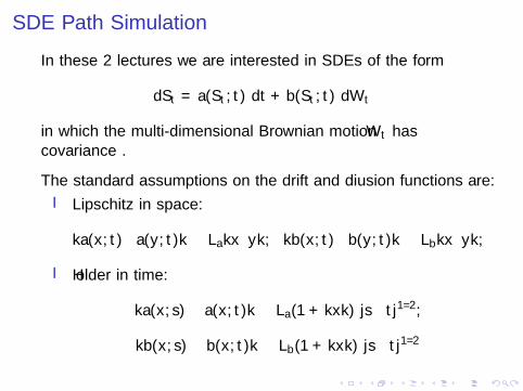
SDE Path Simulation

The simplest approximation is the forward Euler scheme, which isknown as the Euler-Maruyama approximation when applied toSDEs:

Sn+1 = Sn + a(Sn, tn) h + b(Sn, tn) ∆Wn

Here h is the timestep, Sn is the approximation to Snh and the∆Wn are i.i.d. N(0, hΣ) Brownian increments.

For ODEs, the forward Euler method has O(h) accuracy, and othermore accurate methods would usually be preferred.

However, SDEs are very much harder to approximate so theEuler-Maruyama method is used widely in practice.

Numerical analysis is also very difficult and even the definition of“accuracy” is tricky.

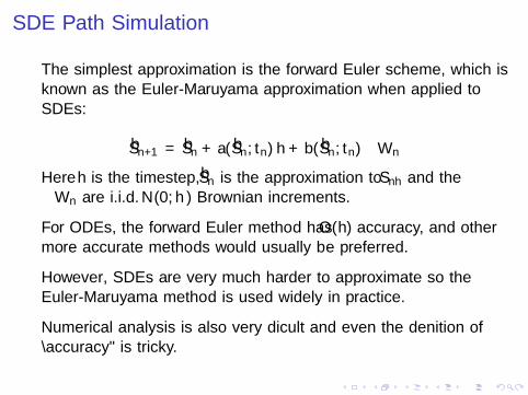
Weak convergence

In many applications, mostly concerned with weak errors, theerror in the expected value of an output quantity of interest (QoI).

If the QoI is f (ST ) this is

E[f (ST )]− E[f (ST/h)]

and it is of order α if

E[f (ST )]− E[f (ST/h)] = O(hα)

For a path-dependent QoI, the weak error is

E[f (S)]− E[f (S)]

where f (S) is a function of the entire path St , and f (S) is acorresponding approximation.

Weak convergence

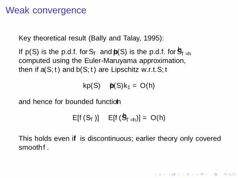
Key theoretical result (Bally and Talay, 1995):

If p(S) is the p.d.f. for ST and p(S) is the p.d.f. for ST/hcomputed using the Euler-Maruyama approximation,then if a(S , t) and b(S , t) are Lipschitz w.r.t. S , t

‖p(S)− p(S)‖1 = O(h)

and hence for bounded function f

E[f (ST )]− E[f (ST/h)] = O(h)

This holds even if f is discontinuous; earlier theory only coveredsmooth f .

Weak convergence

Numerical demonstration: Geometric Brownian Motion

dS = r S dt + σ S dW

r = 0.05, σ = 0.5, T = 1

European call: S0 = 100,K = 110.

Plot shows weak error versus analytic expectation when using 108

paths, and also Monte Carlo error (3 standard deviations)

Weak convergence

10-2

10-1

h

10-2

10-1

Err

or

Weak convergence -- comparison to exact solution

Weak error

MC error

Weak convergence

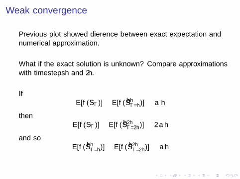
Previous plot showed difference between exact expectation andnumerical approximation.

What if the exact solution is unknown? Compare approximationswith timesteps h and 2h.

IfE[f (ST )]− E[f (Sh

T/h)] ≈ a h

thenE[f (ST )]− E[f (S2h

T/2h)] ≈ 2 a h

and soE[f (Sh

T/h)]− E[f (S2hT/2h)] ≈ a h

Weak convergence

To minimise the number of paths that need to be simulated, bestto use same driving Brownian path when doing 2h and happroximations – i.e. take Brownian increments for h simulationand sum in pairs to get Brownian increments for 2h simulation.

The variance is lower because the h and 2h paths are close to eachother (strong convergence).

This forms the basis for the Multilevel Monte Carlo method

Weak convergence

10-2

10-1

h

10-3

10-2

10-1

Err

or

Weak convergence -- difference from 2h approximation

Weak error

MC error

Strong convergence

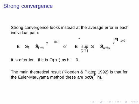
Strong convergence looks instead at the average error in eachindividual path:

(E[(

ST − ST/h

)2])1/2

or

(E

[sup[0,T ]

(St − Sbt/hc

)2])1/2

It is of order β if it is O(hβ) as h→ 0.

The main theoretical result (Kloeden & Platen 1992) is that forthe Euler-Maruyama method these are both O(

√h).

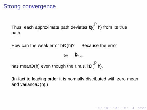
Strong convergence

Thus, each approximate path deviates by O(√h) from its true

path.

How can the weak error be O(h)? Because the error

ST − ST/h

has mean O(h) even though the r.m.s. is O(√h).

(In fact to leading order it is normally distributed with zero meanand variance O(h).)

Strong convergence

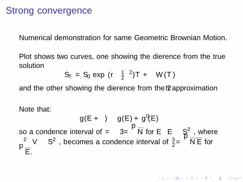
Numerical demonstration for same Geometric Brownian Motion.

Plot shows two curves, one showing the difference from the truesolution

ST = S0 exp((r− 1

2σ2)T + σW (T )

)and the other showing the difference from the 2h approximation

Note that:g(E + δ) ≈ g(E ) + g ′(E ) δ

so a confidence interval of δ=± 3σ/√N for E≡E

[∆S2

], where

σ2≡V[∆S2

], becomes a confidence interval of ±3

2σ/√N E for√

E .

Strong convergence

10-2

10-1

h

10-2

10-1

100

101

Err

or

Strong convergence -- difference from exact and 2h approximation

exact error

MC error

relative error

MC error

Mean Square Error

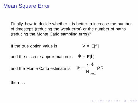
Finally, how to decide whether it is better to increase the numberof timesteps (reducing the weak error) or the number of paths(reducing the Monte Carlo sampling error)?

If the true option value is V = E[f ]

and the discrete approximation is V = E[f ]

and the Monte Carlo estimate is Y =1

N

N∑n=1

f (n)

then . . .

Mean Square Error

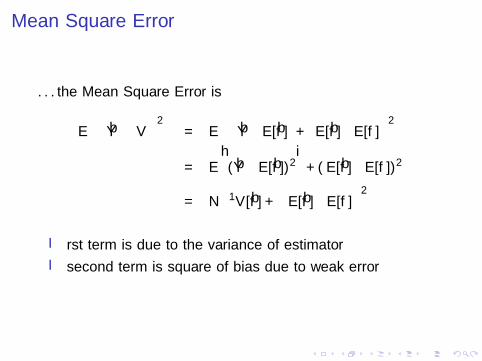
. . . the Mean Square Error is

E[(

Y − V)2]

= E[(

Y−E[f ] + E[f ]−E[f ])2]

= E[(Y−E[f ])2

]+ (E[f ]−E[f ])2

= N−1V[f ] +(E[f ]−E[f ]

)2I first term is due to the variance of estimator

I second term is square of bias due to weak error

Mean Square Error

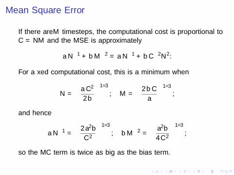
If there are M timesteps, the computational cost is proportional toC = NM and the MSE is approximately

aN−1 + bM−2 = aN−1 + b C−2N2.

For a fixed computational cost, this is a minimum when

N =

(a C 2

2 b

)1/3

, M =

(2 b C

a

)1/3

,

and hence

aN−1 =

(2 a2b

C 2

)1/3

, bM−2 =

(a2b

4C 2

)1/3

,

so the MC term is twice as big as the bias term.

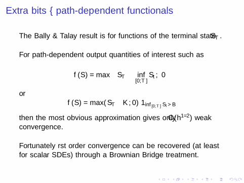
Extra bits – path-dependent functionals

The Bally & Talay result is for functions of the terminal state ST .

For path-dependent output quantities of interest such as

f (S) = max

(ST − inf

[0,T ]St , 0

)or

f (S) = max(ST−K , 0) 1inf [0,T ] St>B

then the most obvious approximation gives only O(h1/2) weakconvergence.

Fortunately first order convergence can be recovered (at leastfor scalar SDEs) through a Brownian Bridge treatment.

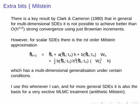
Extra bits – Milstein

There is a key result by Clark & Cameron (1980) that in generalfor multi-dimensional SDEs it is not possible to achieve better thanO(h1/2) strong convergence using just Brownian increments.

However, for scalar SDEs there is the first order Milsteinapproximation

Sn+1 = Sn + a(Sn, tn) h + b(Sn, tn) ∆Wn

+ 12 b(Sn, tn) b′(Sn, tn) (∆W 2

n − h)

which has a multi-dimensional generalisation under certainconditions.

I use this whenever I can, and for more general SDEs it is also thebasis for a very effective MLMC treatment (antithetic Milstein).

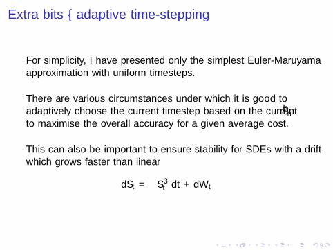
Extra bits – adaptive time-stepping

For simplicity, I have presented only the simplest Euler-Maruyamaapproximation with uniform timesteps.

There are various circumstances under which it is good toadaptively choose the current timestep based on the current Snto maximise the overall accuracy for a given average cost.

This can also be important to ensure stability for SDEs with a driftwhich grows faster than linear

dSt = −S3t dt + dWt

Extra bits – discontinuous drift

Recent research by Muller-Gronbach and Yaroslavtseva(arXiv, 2018) proves that Euler-Maruyama also has O(h1/2)strong convergence for SDEs with a discontinuous drift, such as

dSt = − sign(St) dt + dWt

There are also people researching what happens with discontinuousdiffusion coefficients.

Extra bits – jump-diffusion

Some applications (particularly in finance) use jump-diffusionmodels

dSt = a(St) dt + b(St)dWt + c(S−t )dJt

where J(t) is the number of jumps which have taken place beforetime t, and the jump times are typically modelled as a simplePoisson process.

The Merton model is

dSt = r St dt + σ St dWt + (k−1)S−t dJt

with jump times exponentially distributed with rate λ, and thejump magnitude k Normally distributed.

The numerical treatment of these is usually straightforward – yousimulate the jumps at the jump times, and in between useEuler-Maruyama for the SDE.

Extra bits – Levy processes

Jump-diffusion models have a finite rate of jumping.

A further generalisation is to Levy processes in which there canbe an infinite number of jumps in each time interval, but mostare extremely small.

Exponential Levy models have the form

St = exp(Lt)

where Lt is a Levy process, while Levy driven processes have theform

dSt = a(St) dt + b(St)dLt .

Numerical methods often simulate the big jumps and approximatethe small ones as a Brownian diffusion.

Extra bits – reflected diffusions

In 1D, the simplest reflected diffusion starting from S0 = x ≥ 0 is

St = Wt + x + Lt , Lt ≡ max(− inf[0,t]

Ws − x , 0)

which keeps St ≥ 0.

The multi-dimensional generalisation of this gets more complex,and there is a distinction between normal and oblique reflections.

This class of problems is important in queueing theory, and thereseems to be good potential for further research in this area.

Final Words

I simple Euler-Maruyama method is basis for most Monte Carlosimulation – O(h) weak convergence and O(

√h) strong

convergence

I weak convergence is very important when estimatingexpectations

I strong convergence is usually not important – but is key formultilevel Monte Carlo method to be discussed next

I Mean-Square-Error is minimised by balancing bias due toweak error and Monte Carlo sampling error

Key references

P. Kloeden and E. Platen. “Numerical Solution of StochasticDifferential Equations”. Springer, 1992.

D. Higham. “An algorithmic introduction to numerical simulationof stochastic differential equations”. SIAM Review, 43(3):525-546,2001.

P. Glasserman. “Monte Carlo Methods in Financial Engineering”.Springer, 2003.

S. Asmussen, P.W. Glynn. “Stochastic Simulation: Algorithmsand Analysis”. Springer, 2007.