A measurement of the branching ratio of the

vvK L00 π→ decay

Mikhail Yur’evich DOROSHENKO

March 2005

Department of Particle and Nuclear Physics, School of High Energy Accelerator Science,

The Graduate University for Advanced Science (SOKENDAI), Tsukuba, Ibaraki, Japan

2

Acknowledgments

My first thanks go to Prof. Takao Inagaki, my advisor at the Graduate University for

Advance Science (Sokendai), who spent much of his time to teach me and to help me

accommodate myself in Japan. I am also grateful to his wife, Mrs. Fukoko Inagaki, who has

always been very kind to me.

I would like to thank my Russian adviser, Dr. Alexander Kurilin, who strongly supported

me during this period, and made great efforts together with Prof. Inagaki to make this visit to

Japan possible.

My big thanks go to Prof. Hideki Okuno, who involved me to join the production and

testing of the detectors. Without his organization talent my work for the E391a experiment

would have been much harder. Dr. Yoshio Yoshimura helped me in mechanical work and gave

me good advice. I would like to thank Prof. Takahiro Sato, who participated in my teaching and

Dr. Gei-Youb Lim who always shared his time for discussions and explaining physics to me.

Great thanks go to the Dr. Takeshi Komatsubara for organizing useful seminars about theory and

experimental techniques. Special thanks go to Prof. Taku Yamanaka for his fruitful criticisms in

discussions of new ideas.

I would like to thank Dr. Mitsuhiro Yamaga and Dr. Hiroaki Watanabe who were always

ready to explain to me hard-to-understand points, and discussed with me new ideas. Dr.

Watanabe greatly helped me in writing this thesis. Also, my big thanks go to Ph.D students Mr.

Ken Sakashita and Mr. Toshi Sumida for fruitful discussions and team -work. I am also grateful

to master students from Saga and Osaka Universities, especially, Mr. Shojiro Ishibashi, who

participated in many work and nice evening-parties.

I am grateful to Dr. Evgenii Kuzmin from Joint Institute for Nuclea r research (JINR), who

guided me in constructing of the detectors, and taught me necessary software techniques. He

showed me the way how to reach the goal. I would like to thank the JINR team for fruitful team-

work.

My special thanks go to Elene Podolskoi, who greatly supported me during my stay in

Japan, and especially during writing the thesis. I could complete the thesis during a tight period

thanks to her.

This work was supported by a grant of the Japanese government.

3

Abstract

The vvKL00 π→ decay is a golden channel to study the origin of CP violation. The

branching ratio is proportional to the parameter η, which measures the magnitude of the CP

violation in the CKM matrix; the theoretical uncertainties are so small that the measurement

allows us to make a precise test of the Standard Model of CP violation.

Experiment E391a was designed to measure vvK L00 π→ decay with a goal of 10103 −⋅ single -

event sensitivity. A vvK L00 π→ decay is searched for by a signal of 00 π→LK ( γγπ →0 ) +

nothing. The energies and positions of the gammas were measured with a CsI calorimeter. The

“nothing” was confirmed by no additional signals in the veto system, which covered the whole

decay region. Several unique techniques were developed for E391a , such as a well-collimated

“pencil” beam, differential pumping, a double-decay chamber and highly sensitive veto detectors

to cover almost the whole 4π geometry.

During the beam time in February-June 2004, we collected a bout 6Tb of data, equivalent to

a full 60 days of operation. As the first step, we performed an analysis of one day of data, which

is a main topic of the present thesis. Good quality and stability of the data were confirmed by this

analysis. All detectors were calibrated by using punch-through and/or cosmic muons. In addition,

the CsI calorimeter was calibrated more precisely by using γ’s from the 0π ’s produced with an

aluminum target. The reconstruction of neutral decays ( γγππ ,2,3 000 →LK ) showed good

agreement with MC simulations and in the number of the 0LK yield. The pure signal and

background samples of γγππ ,2,3 000 →LK were used for a veto study, and showed good

agreement of the acceptance loss due to the veto cuts.

In the 2γ sample, which contains candidates for vvKL00 π→ decays, we observed various

sources of background events surrounding the signal box. They were from the other 0LK decays

and from halo neutron interactions; in addition, we found a clear effect due to the interactions of

the beam-core neutrons with the membrane separating the tw o vacuum chambers, which fell

down into the beam axis, accidentally.

Finally, we opened the signal box and observed no event inside. The single -event

sensitivity for vvK L00 π→ decay was estimated to be 8.3x10-7. This led to an upper limit of the

branching ratio of 6109.1 −⋅ at the 90% confidence level.

We conclude that the analysis of the one -day data was very valuable to understand the

performance of the experiment and to develop new software techniques for the analysis. The

results of this study were reflected in an upgrade of the experimental setup for the next run, RUN

II, which started in the middle of January, 2005.

4

Contents 1. Motivation of experiment

1.1. Theoretical background 1.1.1. General 1.1.2. vvK L

00 π→ decay in the Standard Model 1.1.3. vvK L

00 π→ decay beyond the Standard Model 1.2. Current status of other experiments 1.3. Motivation of the one-day analysis

2. Experimental method 2.1. Detection method

2.1.1. Setup 2.1.2. Pencil beam 2.1.3. High vacuum in the decay volume 2.1.4. Double-decay chamber 2.1.5. Highly sensitive veto system

2.2. Apparatus 2.2.1. Overview 2.2.2. Beam line 2.2.3. CsI calorimeter

2.2.3.1. Overview 2.2.3.2. CsI modules 2.2.3.3. Cooling system

2.2.4. Main and front barrels 2.2.4.1. Main barrel 2.2.4.2. Barrel charge veto 2.2.4.3. Front barrel 2.2.4.4. Assembling of modules

2.2.5. Collar counters and beam anti(BA) 2.2.6. Vacuum system

2.2.6.1. Overview 2.2.6.2. Scheme of pumping 2.2.6.3. Bench tests of the membrane

3. Data taking in physics run 3.1. DAQ system

3.1.1. Overview 3.1.2. Electronics 3.1.3. Trigger logic 3.1.4. Server computer and network 3.1.5. DAQ performance

3.2. Data taking in 2004 physical run 3.2.1. Triggers during physical data taking 3.2.2. Data taking

5

4. Calibrations of the detectors 4.1. Pedestals 4.2. Gain monitoring system (Xenon/LED) 4.3. Energy calibration of the CsI calorimeter

4.3.1. Calibration by cosmic muons 4.3.2. Calibration by punch-through muons 4.3.3. Comparison of the gain factors obtained by cosmic muons and punch-through

muons 4.3.4. Calibration by 0π ’s produced on an aluminum target

4.4. Energy calibration of the veto detectors 4.4.1. CC03 and sandwich counters 4.4.2. Collar counters (CC02,4,5,6,7) 4.4.3. Main charge veto 4.4.4. Main barrel and barrel charge veto 4.4.5. Beam catcher and beam charge veto

4.5. Timing calibration of the CsI calorimeter 5. Analysis

5.1. Data skimming 5.2. Kinematical reconstruction

5.2.1. Hit position of γ 5.2.2. Energy of γ 5.2.3. Decay vertex 5.2.4. Momentum correction

5.3. Reconstruction of the neutral decay modes 5.3.1. Introduction. 5.3.2. Online veto 5.3.3. MC simulation 5.3.4. Reconstruction of γγπ →0 decays (candidates of vvKL

00 π→ ) 5.3.4.1. Contributions of the neutral 0

LK decays 5.3.4.2. Contribution of the 00 πππ −+→LK decays 5.3.4.3. Halo neutrons 5.3.4.4. Beam core neutrons 5.3.4.5. Optimization of the kinematical cuts

o Cluster shape analysis o Distance and energy balance of gammas

5.3.5. Normalization channels 5.3.5.1. 6γ events and reconstruction of 00 3π→LK 5.3.5.2. 4γ events and reconstruction of 00 2π→LK 5.3.5.3. 2γ events and reconstruction of γγ→0

LK 5.3.5.4. Comparison of the branching ratios among three neutral decay

modes

6

5.4. Study of the veto counters 5.4.1. Pure signal and background samples ( γγππ ,2,3 000 →LK ) 5.4.2. Veto study of each detector

5.4.2.1. Main barrel (MBR) 5.4.2.2. CC03 5.4.2.3. CC02 5.4.2.4. Front barrel 5.4.2.5. CC04,CC05,CC06,CC07 5.4.2.6. Charge layers of the CC04 and CC05, Beam hole counter and Main

Charge Veto(CHV) 5.4.2.7. Beam anti detector 5.4.2.8. Summary

5.5. Study of the vvK L00 π→ decays

5.5.1. Candidate for vvK L00 π→ decays

5.5.2. Box opening and acceptance estimation

5.6. Results 5.7. Discussion

6. Conclusion

7

Chapter 1

Motivation of the experiment

1.1 Theoretical background

The asymmetry between a particle and its anti-particle, which is called CP violation, was

discovered in the neutral K-meson system in 1964 [1]. On the macroscopic scale, CP violation is

necessary to explain matter domination in the universe. On the microscopic scale, it has been an

important guide to understand elementary-particle interactions. The origin of CP violation,

however, is still not clear. Notably, the Koboyashi-Maskawa model, the Standard Model (SM) of

elementary particles, does not give strong enough CP violation effects to explain matter

domination in the universe. In order to uncover the origin of CP violation, it is important to test

predictions of the Kobayashi-Maskawa model. Measurements of direct CP violation processes

are especially important, since they offer power to discriminate various theoretical models.

Experiments for studying of CP violation using K-mesons have been actively pursued,

because K-mesons are easy to generate, and their CP sensitivity is high [1]. Similar to the K-

meson system, the B-meson system also has a high sensitivity for CP violation. Recently, B-

8

factory experiments, such as KEK-BELLE and SLAC-BABAR, have confirmed large CP

violation in the B-meson system [2] , where the validity of the KM model has been established by

observing the predicted indirect CP violation in the B-meson system due to mixing phenomena.

On the other hand, it is not yet clear if direct CP violation in B-meson decays is consistent with

the KM-model predictions.

We believe that the E391 experiment, which is searching for the vvKL00 π→ decay [3], will

shed light on the validity of the KM model and in the search for a new source of CP violation in

Nature. According to the Standard Model, the branching ratio of the vvKL00 π→ decay is

predicted to be 3x10-11.[4]. The vvKL00 π→ decay measurement can unambiguously determine

the height, η, of the unitarity triangle of the fundamental CKM (Cabibbo-Kobayashi-Maskawa)

parameters, because this process is theoretically very clean. On the other hand, the experiment of

B-meson decays can measure the angle, φ 1(β) , of the unitarity triangle. Therefore, it is possible

to test the KM Model and to search for a new source of CP violation by combining all of the

experimental results from K-meson and B-meson decays.

CP violation arises naturally in the three-generation Standard Model [5]. CP violation in

the Standard Model appears only in the charged-current interactions of quarks, and is described

by only one complex phase, the Kobayashi-Maskawa phase. First, a brief summary of CP

violation in the KM model is described. Then, the physics of the vvKL00 π→ decay is discussed.

1.1.1 General

The Lagrangian of the weak charged-current interactions of quarks is written as follows:

( )( )−++ ⋅+⋅= µµ

µµ γγ WuVdWdVu

gL LCKMLLCKMLCC 2

2 , (1.1)

where

( )tcuu ,,= ,

=

bs

d

d .

CKMV is the Cabibo-Koboyashi-Maskawa unitary matrix, 2g is the weak-coupling constant and

µγ are the Dirac matrices. The subscript L denotes “left-handed” spinors; ( )qqL 5121

γ−≡ . The

symbols u, d, s, c, b and t denote the quark mass eigenstate s of each flavor.

9

The Lagrangian changes under the CP transformation as follows:

( )+− ⋅+⋅= µµ

µµ γγ WdVuWuVdgLCP LCKMLL

TCKMLCC

*2 )()(2

)( . (1.2)

Therefore, if *)( CKMCKM VV ≠ , that is, if the CKM matrix contains an imaginary parameter ,

which cannot be absorbed by re -phasing of the quark fields, CP symmetry is violated in the weak

charged-current interactions of quarks.

A unitary nn × matrix for n quark generations is characterized by 2/)1( −= nnnθ rotation

angles and 2/)2)(1( −−= nnnδ physical phases. For 2=n , only the Cabibbo angle remains,

since we have 1=θn and 0=δn . For three generations, we have 3=θn and 1=δn . Therefore,

one CP phase in CKMV appears.

From the Lagrangian, the weak eigenstate of quarks is described by a mixed state of the

mass eigenstates of quarks with the 33× matrix, CKMV . Since CKMV is not diagonal, the ±W

boson can couple to quarks of different generations.

Wolfenstein parameterization of the CKM matrix in terms of four parameters

(λ, Α, ρ and η) is convenient, because it help us to estimate the hierarchy of the magnitudes of

the matrix elements[6]:

=

tbtstd

cbcscd

ubusud

CKM

VVV

VVVVVV

V

( )4

23

22

32

1)1(2/1

)(2/1

λληρλ

λλλ

ηρλλλ

OAiA

A

iA

+

−−−−−

−−

≈ , (1.3)

where ( ) cc θθλ ,sin≡ is the Cabibo angle. The parameter η represents the imaginary component

of CKMV in the Wolfenstein parameterization.

Our present knowledge of the CKM matrix elements comes from the following sources:

• udV =0.9738 ± 0.0005 [7]. The value was derived from two distinct sources:

the nuclear beta decays [8] and the decay of free neutrons [9]

• usV =0.2200 ± 0.0026 [10]. It was obtained from 3eK decays [11] with

various corrections [12,13]

• cdV =0.224 ± 0.012 [10]. It was deduced from neutrino and antineutrino

production of charm quark off valence d quarks [14-16]

10

• csV =0.996 ± 0.013 [13]. It was obtained from direct measurements of the

charm-tagged W decays [12]. However, the most precise value was derived

from measurements of the branching fraction of the leptonic decays of the W

boson [13].

• ( ) 3105.13.41 −⋅±=cbV [17]. It was extracted from exclusive measurements of

lvDB *→ decays and the inclusive one using the semileptonic width of

vXlB → decays.

• ( ) 31047.067.3 −⋅±=ubV [18]. The world average was calculated as the

weighted mean from inclusive and exclusive measurements of ulvb →

decays of B mesons.

• )24.0,31.0(94.0222

2

−+=++ tbtstd

tb

VVV

V [19]. This constraint was obtained

from a study of the branching fraction of vblt +→ decays.

The remain ing CKM matrix elements were calculated using the unitarity condition,

1=⋅ +CKMCKM VV . (1.4)

In the Wolfenstein parameterization, the parameters were determined as follows [14] (in brackets

the relative errors are shown) :

0026.02200.0 ±=λ (1.1%),

037.0853.0 ±=A (4.3%),

09.020.0 ±=ρ (4.5%),

05.033.0 ±=η (15%),

where ( )2/1 2λρρ −= and ( )2/1 2ληη −= . Thus the most ambiguous parameter is η , which ha s a

15% relative error.

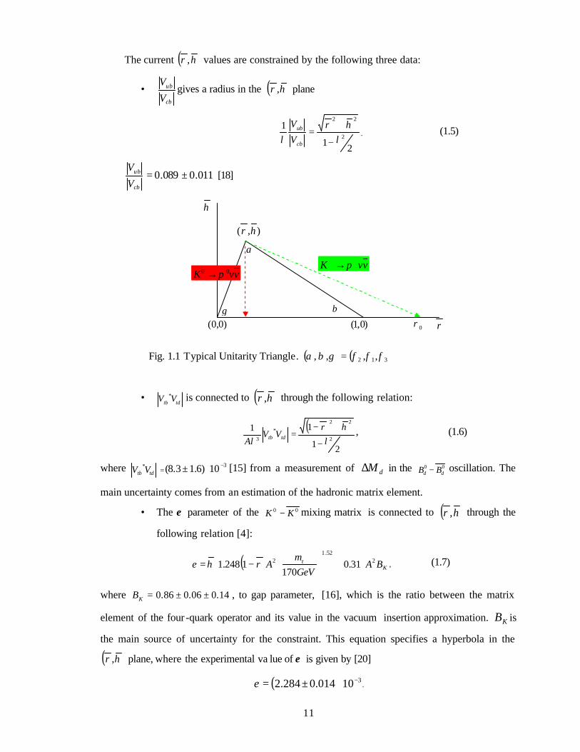
The unitarity of CKMV can be visually expressed as a triangle, “Unitarity Triangle”. Fig. 1.1

shows one of the typical Unitarity Triangle s. If all CP violation phenomena can be explained by

the Standard Model, the Unitarity Triangle is strictly closed. On the other hand, if the Unitarity

Triangle is not closed, there is new physics beyond the Standard Model. Since the relative

importance of the new physics effects may be different for each process, precise measurements

of various CKM parameters should be the keys to identify any new source of CP violation.

11

The current ( )ηρ, values are constrained by the following three data:

• cb

ub

V

Vgives a radius in the ( )ηρ, plane

21

12

22

ληρ

λ −

+=

cb

ub

V

V. (1.5)

cb

ub

V

V = 011.0089.0 ± [18]

Fig. 1.1 Typical Unitarity Triangle. ( ) ( )312 ,,,, φφφγβα =

• tdtb VV *

is connected to ( )ηρ, through the following relation:

( )

21

112

22

*

3 ληρ

λ −

+−=tdtb VV

A, (1.6)

where tdtb VV *

=310)6.13.8( −⋅± [15] from a measurement of dM∆ in the 00

dd BB − oscillation. The

main uncertainty comes from an estimation of the hadronic matrix element.

• The ε parameter of the 00 KK − mixing matrix is connected to ( )ηρ, through the

following relation [4]:

( ) Kt BA

GeVm

A 252.1

2 31.0170

1248.1

+

−= ρηε , (1.7)

where 14.006.086.0 ±±=KB , to gap parameter, [16], which is the ratio between the matrix

element of the four -quark operator and its value in the vacuum insertion approximation. KB is

the main source of uncertainty for the constraint. This equation specifies a hyperbola in the

( )ηρ, plane, where the experimental va lue of ε is given by [20]

( ) 310014.0284.2 −⋅±=ε .

ρ

η

)0,1(

),( ηρ

)0,0( 0ρ

vvK ++ →π

βγ

α

vvK 00 π→

12

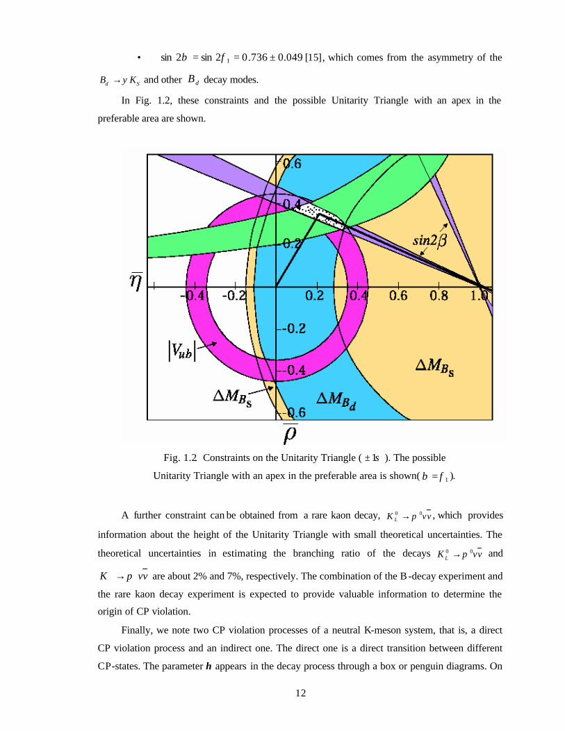
• 049.0736.02sin2sin 1 ±== φβ [15], which comes from the asymmetry of the

Sd KB ψ→ and other dB decay modes.

In Fig. 1.2, these constraints and the possible Unitarity Triangle with an apex in the

preferable area are shown.

Fig. 1.2. Constraints on the Unitarity Triangle ( σ1± ). The possible

Unitarity Triangle with an apex in the preferable area is shown ( 1φβ = ).

A further constraint can be obtained from a rare kaon decay, vvK L00 π→ , which provides

information about the height of the Unitarity Triangle with small theoretical uncertainties. The

theoretical uncertainties in estimating the branching ratio of the decays vvK L00 π→ and

vvK ++ →π are about 2% and 7%, respectively. The combination of the B -decay experiment and

the rare kaon decay experiment is expected to provide valuable information to determine the

origin of CP violation.

Finally, we note two CP violation processes of a neutral K-meson system, that is, a direct

CP violation process and an indirect one. The direct one is a direct transition between different

CP-states. The parameter η appears in the decay process through a box or penguin diagrams. On

13

the other hand, the indirect one appears in decays into the same CP-state , which is produced by

00 KK − oscillation. In the case of indirect CP violation, the η parameter appears in the

oscillation process.

1.1.2 vvK L00 π→ decay in the Standard Model

In this section, the theoretical bases of the vvKL00 π→ decay within the Standard Model,

namely the branching ratio prediction and its relation to the parameter η , are described.

The vvKL00 π→ decay offers one of the most transparent probes concerning the origin of

CP violation. It proceeds through the diagrams shown in Fig. 1. 3.

Fig. 1.3. D iagrams of the vvK L00 π→ decay

14

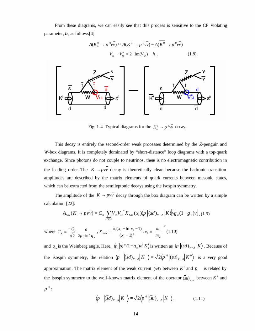
From these diagrams, we can easily see that this process is sensitive to the CP violating

parameter, η, as follows[4]:

)()()( 000000 vvKAvvKAvvKA L πππ →−→≈→

η∝⋅=−∝ )Im(2*tdtdtd VVV , (1.8)

Fig. 1.4. Typical diagrams for the vvKL

00 π→ decay.

This decay is entirely the second-order weak processes determined by the Z-penguin and

W-box diagrams. It is completely dominated by “short-distance” loop diagrams with a top-quark

exchange. Since photons do not couple to neutrinos, there is no electromagnetic contribution in

the leading order. The vvK π→ decay is theoretically clean because the hadronic transition

amplitudes are described by the matrix elements of quark currents between mesonic states,

which can be extracted from the semileptonic decays using the isospin symmetry.

The amplitude of the vvK π→ decay through the box diagram can be written by a simple

calculation [22]:

[ ]∑=

− −=→tci

aAViboxisidKbox vvKdsxXVVCvvKA,

5* )1()()()( γγππ , (1.9)

where w

FK

GC

θπα

2sin22

−≡ ,

2)1()1ln(

−−−

=i

iiibox x

xxxX ,

2

≡

w

ii m

mx (1.10)

and wθ is the Weinberg angle. Here, Kds a )1( 5γγπ − is written as Kds AV −)(π . Because of

the isospin symmetry, the relation 00 )(2)( KusKds AVAV −+

−+ = ππ is a very good

approximation. The matrix element of the weak current )( ds between K+ and +π is related by

the isospin symmetry to the well-known matrix element of the operatorAV

us−

)( between K+ and

0π :

+−

+−

+ = KusKds AVAV )(2)( 0ππ . (1.11)

15

The matrix element of the operator AV

us−

)( is measured in veK ++ → 0π decays. The amplitude

for this transition is given by

[ ]evKdsVG

veKA aAVusF

e )1()(2

)( 500 γγππ −=→ +

−++ . (1.12)

By using the veK ++ → 0π data, the branching ratio of vvK ++ → π is expressed as

2

42

20

sin2)()(

→=→ ++++

λθπαππ

DveKBvvKB

we , (1.13)

where ∑=

=tci

iisid xXVVD,

* )( .

We can express the amplitude of vvK L00 π→ decay as

)()()( 002

001

00 vvKAvvKAvvKA L ππεπ →+→=→ , (1.14)

where K1 and K2 are CP even and odd states, respectively. The an amplitudes of K1 and K2

decays are written as follows:

[ ] )15.1(),(Re)()(2

1)( 0000001 vvKAvvKAvvKAvvKA ++ →=→+→=→ ππππ

[ ] )16.1(),(Im)()(2

1)( 0000002 vvKAivvKAvvKAvvKA ++ →=→−→=→ ππππ

Since the CP parity of 01K is even, which is the same as that of the vv0π system, the amplitude

of vvK 001 π→ contributes to the process through indirect CP violation in the 00 KK − oscillation

proportional to the parameter ε .

From the above equations, the branching ratio can be approximated as a sum over the

contribution from indirect and direct CP-violationprocess,

[ ])()1()(1073.2)( 422501 tcindirect xXAxXvvKBr ρλεπ −+⋅≈→ − , (1.17)

[ ])(1073.2)( 42502 tdirect xXAvvKBr ηλπ −⋅≈→ . (1.18)

Since ε is small, ~10-3, the indirect contribution is negligibly small. The charm

contribution, which gives rise to some theoretical ambiguity, is small because the charm term is

significant only in the indirect contribution. This is the reason why the theoretical ambiguity is

small for vvK L00 π→ decay, as compared to vvK ++ → π decay.

By adding the Z-penguin diagrams, the )( ixX function given by Inami and Lim[23] is

−

++

−−

=1

2)2(63

8)(

2i

i

i

iii x

xx

xxxX . (1.19)

16

The SM prediction is hence

)20.1(,10)1.18.2(1008.4)()( 112410001

00 −− ⋅±=⋅=→≈→ ηππ AvvKBrvvKBr directL

Isospin-symmetry-violating quark mass effects and the electroweak radiative corrections

reduce this branching ratio by 5.6%.[24] . Next-to-leading order QCD effects are known with an

accuracy of ± 1.1%[25]. The overall theoretical uncertainty is estimated to be below 2%.

Finally, the theoretical features of vvKL00 π→ decay in the Standard Model are summarized

as follows:

• The branching ratio is predicted to be (2.8 ± 1.1)10-11, which is quadratically

proportional to the CP violation parameter, η.

• The direct CP violating processes are dominating. The contribution of the indirect CP

violating processes is about 10-4 of the contribution of the direct processes.

• The ambiguity in the theoretical prediction is very small, ~1 %, which is much

smaller than that of the vvK ++ → π decay due to the small charm contribution.

1.1.3 vvK L00 π→ decay beyond the Standard Model

There are many models beyond the Standard Model (BSM). The predictions for the

vvKL00 π→ branching ratio by various BSM models of CP violation process are listed in Table

1.1. These models are classified into three classes: SUSY (supersymmetry) models, extended

Higgs models and models with new fermions.

One feature of these BSM models is that the number of CP phases is increased. These new

phases generally contribute to additional diagrams. Therefore, whether the BSM models has 4th

generation, extra "vector-like" quarks, L-R (left-right) symmetry or many Higgs bosons, the

branching-ratio prediction tends to be larger than that of the Standard Model. For SUSY models,

the scale of ε Κ gives a strong constraint among additional CP phases, such that they tend to

predict a branching ratio that is almost the same as that predicted by the Standard Model. On the

other hand, a larger effect from the SUSY CP phases is expected for the Sd KJB ψ/→ decay.

Therefore, the Unitarity Triangle can become inconsistent between the Sd KJB ψ/→ and

vvKL00 π→ decays. From the pattern of inconsistency, there is a possibility to identify the

specific BSM model.

17

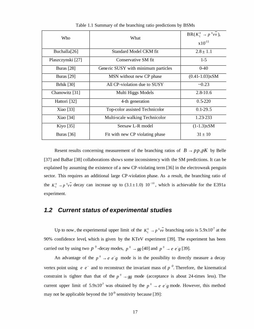
Table 1.1 Summary of the branching ratio predictions by BSMs

Who What BR( vvK L

00 π→ ),

x10-11

Buchalla[26] Standard Model CKM fit 2.8 ± 1.1

Plaszczynski [27] Conservative SM fit 1-5

Buras [28] Generic SUSY with minimum particles 0-40

Buras [29] MSN without new CP phase (0.41-1.03)xSM

Brhik [30] All CP-violation due to SUSY ~0.23

Chanowitz [31] Multi Higgs Models 2.8-10.6

Hattori [32] 4-th generation 0.5-220

Xiao [33] Top-color assisted Technicolor 0.1-29.5

Xiao [34] Multi-scale walking Technicolor 1.23-233

Kiyo [35] Seesaw L-R model (1-1.3)xSM

Buras [36] Fit with new CP violating phase 31 ± 10

Resent results concerning measurement of the branching ratios of KB πππ,→ by Belle

[37] and BaBar [38] collaborations shows some inconsistency with the SM predictions. It can be

explained by assuming the existence of a new CP-violating term [36] in the electroweak penguin

sector. This requires an additional large CP-violation phase. As a result, the branching ratio of

the vvK L00 π→ decay can increase up to 1010)0.11.3( −⋅± , which is achievable for the E391a

experiment.

1.2 Current status of experimental studies

Up to now, the experimental upper limit of the vvKL00 π→ branching ratio is 5.9x10-7 at the

90% confidence level, which is given by the KTeV experiment [39]. The experiment has been

carried out by using two 0π -decay modes, γγπ →0 [40] and γπ −+→ ee0 [39].

An advantage of the γπ −+→ ee0 mode is in the possibility to directly measure a decay

vertex point using −+ee and to reconstruct the invariant mass of π 0. Therefore, the kinematical

constraint is tighter than that of the γγπ →0 mode (acceptance is about 24-times less). The

current upper limit of 5.9x10-7 was obtained by the γπ −+→ ee0 mode. However, this method

may not be applicable beyond the 10-9 sensitivity because [39]:

18

• the branching ratio of the γπ −+→ ee0 decay is small, ~1%.

• the final state in the radiative veK L γπ m±→0 decay looks like γπ −+→ ee0 + nothing if

±π is misidentified as ±e . Since the branching ratio of veK L γπ m±→0 decay is as

large as 3.62x10-3, the miss-identification probability for ±π must be below 10-10,

which seems to be difficult to achieve.

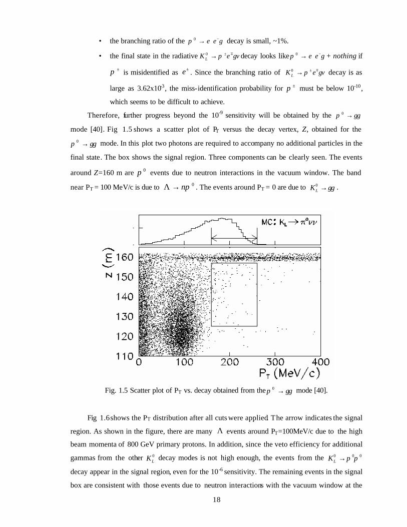
Therefore, further progress beyond the 10-9 sensitivity will be obtained by the γγπ →0

mode [40]. Fig 1.5 shows a scatter plot of PT versus the decay vertex, Z, obtained for the

γγπ →0 mode. In this plot two photons are required to accompany no additional particles in the

final state. The box shows the signal region. Three components can be clearly seen. The events

around Z=160 m are 0π events due to neutron interactions in the vacuum window. The band

near PT = 100 MeV/c is due to 0πn→Λ . The events around PT = 0 are due to γγ→0LK .

Fig. 1.5 Scatter plot of PT vs. decay obtained from the γγπ →0 mode [40].

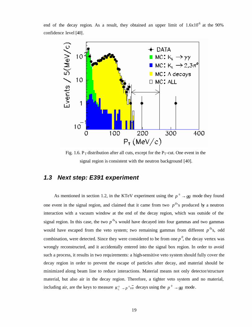
Fig 1.6 shows the PT distribution after all cuts were applied. The arrow indicates the signal

region. As shown in the figure, there are many Λ events around PT=100MeV/c due to the high

beam momenta of 800 GeV primary protons. In addition, since the veto efficiency for additional

gammas from the other 0LK decay modes is not high enough, the events from the 000 ππ→LK

decay appear in the signal region, even for the 10-6 sensitivity. The remaining events in the signal

box are consistent with those events due to neutron interactions with the vacuum window at the

19

end of the decay region. As a result, they obtained an upper limit of 1.6x10-6 at the 90%

confidence level [40].

Fig. 1.6. P T distribution after all cuts, except for the PT-cut. One event in the

signal region is consistent with the neutron background [40].

1.3 Next step: E391 experiment

As mentioned in section 1.2, in the KTeV experiment using the γγπ →0 mode they found

one event in the signal region, and claimed that it came from two π0’s produced by a neutron

interaction with a vacuum window at the end of the decay region, which was outside of the

signal region. In this case, the two π 0’s would have decayed into four gammas and two gammas

would have escaped from the veto system; two remaining gammas from different π 0’s, odd

combination, were detected. Since they were considered to be from one π 0, the decay vertex was

wrongly reconstructed, and it accidentally entered into the signal box region. In order to avoid

such a process, it results in two requirements: a high-sensitive veto system should fully cover the

decay region in order to prevent the escape of particles after decay, and material should be

minimized along beam line to reduce interactions. Material means not only detector/structure

material, but also air in the decay region. Therefore, a tighter veto system and no material,

including air, are the keys to measure vvK L00 π→ decays using the γγπ →0 mode.

20

One more important point is a narrow beam (‘pencil beam’). Because the decay vertex is

reconstructed on the beam axis, the reconstructed transverse momentum of 0π is smeared due to

the size of the beam. Better PT resolution is crucial to discriminate the background, because

many sources, such as multi-body decay, odd combination and hyperon decay, produce

background in the lower PT region. Although a narrow beam is better for background rejection,

but there is a competing process that restricts the size of the beam. If we collimate the beam into

a small size, the K0L flux is reduced. An optimum point should be chosen.

In the KTeV experiment an average K0L momentum was about 70 GeV/c . Even after a long

flight of 90 m from target, the beam contained hyperons. They could easily produce π 0 in the

decay region. It is serious background because the neutron, which is the other decayed participle,

is hard to be detected. Since hyperons have a short lifetime compared with K0L, their flux

surviving at the detector region decreases with a decrease of the beam momentum. A smaller

momentum of K0L can reduce such backgrounds.

The E391 experiment was proposed in 1996 to search of the vvK L00 π→ decay at a single -

event sensitivity of 3x10-10. All hints from the KTeV experiment mentioned above are realized in

E391 setup. The veto system fully covers the decays region. The background decays at the

entrance of the decay region is suppressed by a long additional decay chamber installed before

the main decay chamber. A high vacuum is reached by separating of the decay region and the

detector region by a thin membrane, and separated evacuation systems for two vacuum regions

are used. Vacuum windows are located far from the decay region. The beam is collimated within

2 mrad by the system of 6 collimators. The average K0L momentum is about 2 GeV/c. A deta iled

description of the apparatus is presented in chapter 2.

1.4 Motivation of the one day analysis

We had runs for about 100 days, and took physics data for about 60 days. We then

performed a detail analysis of a one -day data sample, which is reported in this thesis. A careful

analysis of a small fraction of the data is very valuable for understanding the quality of the data ,

and for setting up a working strategy for further analysis. Since the sensitivity obtained from the

one-day sample is expected to be comparable with that of the previous KTeV experiment, the

result will be a good starting point. Any problems that we encounter in the one-day analysis will

guide us to more a effective strategy for processing a large data sample in the future. The MC

tools and the reconstruction routines can be checked critically in this analysis. The data

skimming process is one of the crucial tools to be developed and tested. Moreover, we can

21

examine the consistency between our expectations and reality. Unexpected phenomena may

appear beyond our expectations.

In summary, an analysis of the one-day sample is very valuable for the first overall check

of the E391a experiment at a comparable sensitivity with that of KTeV. Since the data size is not

very big and can be processed within a reasonable time , it is convenient for developing and

testing reconstruction routines. Further analysis of large samples, as well as modifications of the

experimental setup in successive runs, will be done based on knowledge obtained from this one-

day analysis.

22

Chapter 2

Experimental method

2.1 Detection method

The vvKL00 π→ decay is planned to be observed by a signal of 00 π→LK ( γγπ →0 ) +

nothing. The energies and positions of two photons are measured with a CsI calorimeter. The

“nothing” is confirmed by no additional signals in a veto system that covers the whole K0L decay

region.

All background K0L decays have additional photons or charged particles , which can be

detected by the veto system. Although the γγ→0LK decay has no additional particles, it can be

discriminated from the vvKL00 π→ decay using transverse momentum and acoplanarity angle

cuts.

Since the CsI calorimeter measures two γ’s positively, precise energy and position

determinations of γ are important to identify the vvKL00 π→ decay. In addition, a precise hit-

timing measurement is mandatory to reject accidental hits in the CsI calorimeter. An undoped-

23

CsI crystal, which has a moderate light output and a fast time response, is one of the best

materials to meet these requirements.

2.1.1. Setup

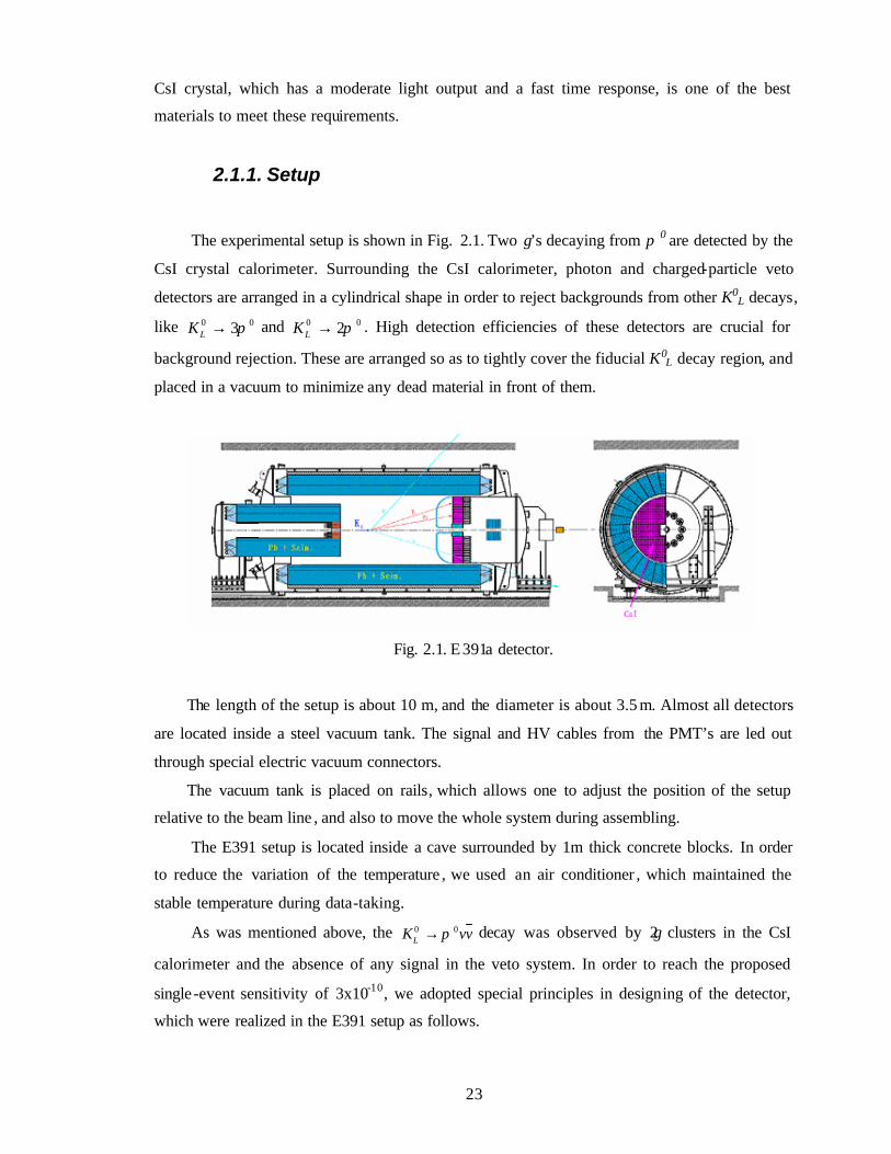
The experimental setup is shown in Fig. 2.1. Two γ’s decaying from π 0 are detected by the

CsI crystal calorimeter. Surrounding the CsI calorimeter, photon and charged-particle veto

detectors are arranged in a cylindrical shape in order to reject backgrounds from other K0L decays,

like 00 3π→LK and 00 2π→LK . High detection efficiencies of these detectors are crucial for

background rejection. These are arranged so as to tightly cover the fiducial K0L decay region, and

placed in a vacuum to minimize any dead material in front of them.

Fig. 2.1. E391a detector.

The length of the setup is about 10 m, and the diameter is about 3.5 m. Almost all detectors

are located inside a steel vacuum tank. The signal and HV cables from the PMT’s are led out

through special electric vacuum connectors.

The vacuum tank is placed on rails, which allows one to adjust the position of the setup

relative to the beam line , and also to move the whole system during assembling.

The E391 setup is located inside a cave surrounded by 1m thick concrete blocks. In order

to reduce the variation of the temperature , we used an air conditioner , which maintained the

stable temperature during data-taking.

As was mentioned above, the vvKL00 π→ decay was observed by 2γ clusters in the CsI

calorimeter and the absence of any signal in the veto system. In order to reach the proposed

single -event sensitivity of 3x10-10, we adopted special principles in designing of the detector,

which were realized in the E391 setup as follows.

24

2.1.2. Pencil beam

In the vvKL00 π→ decay, only two γ’s as a product of the π 0 decay are detectable. A

measurement of the direction of γ is not so easy, and only the energy and the hit position can be

measured with good accuracy. Without direction measurements of γ’s, the decay vertex can be

obtained with an assumption that two γ’s come from π 0. In this case, there still remains an

ambiguity of the vertex position in the transverse direction. It is thus required to assume that the

decay vertex is on the beam axis. This results in a requirement concerning the very small size of

the beam cross section.

In the E391 experiment, we used a so-called ‘pencil beam’. A system of collimators selects

only a 2 mrad angle from the target, so that at the exit of the last collimator, C6, the radius of the

core beam is about 2 cm. At the calorimeter position (~18 m from the target), the radius of the

core beam is less than 4 cm. A halo of the beam is suppressed by more than 5 orders of

magnitude relative to the beam core intensity, as described in 2.2.2.

2.1.3. High vacuum in a decay volume

From a MC study of the interaction of neutrons with air, it was found that the background

contribution is less than 0.1 events at a vacuum pressure of 10-5 Pa for a sensitivity of 3x10-11 for

the vvK L00 π→ decay. Since the E391a experiment proposes to reach a sensitivity of 3x10-10, a

vacuum higher than 10-4 Pa is required in order to reduce the background down to a negligible

level (< 0.1 events).

In the E391 setup, almost all detectors are located inside of the vacuum region. This makes

it hard to reach the required vacuum level of ~ 10-4 Pa, or better, because of out-gassing from

large a lead-scintillator sandwich detectors. We adopted the solution of differential pumping, in

which a low vacuum region containing detectors and a high vacuum decay volume are separated

with a thin membrane of 20 mg/cm2 thickness. Each vacuum level is maintained by a different

evacuation system, namely by the mechanical booster pumps for the low-vacuum region and by

the turbo-molecular pumps for the high-vacuum region.

25

2.1.4. Double decay chamber

The background events from the other decays may appear in a signal box of the vvKL00 π→

decay due to additional particles escaping from the veto system. We tightly cover almost all of

the decay volume with a 4π geometry by veto detectors. However, if the K0L decay occurs at the

entrance of the decay volume, the particles can escape back from the veto system. In order to

avoid this situation we developed an additional decay chamber before the main decay volume.

Decays occurring in the first decay volume are rejected by a front barrel veto detector

surrounding the beam axis and the CC02 counter located at the end of the first decay volume.

The γ’s going forward are suppressed by a small beam hole of CC02. If a decay occurs at the

border between the first and the main decay volumes, the possibility for γ’s to escape in the

backward direction along the beam line is suppressed by a long (2.75 m) front barrel veto

detector.

2.1.5. Highly-sensitive veto system

The K0L decay, which may become a main background source , is 00 2π→LK decay, where

two γ’s from the π 0 decay hit the CsI calorimeter and remaining γ’s are not detected by the veto

system. The branching ratio of this decay is 9.27x10-4, which is about 8 orders higher than that of

the vvKL00 π→ decay. This results in a requirement of the inefficiency of the veto system to be

level of about 10-4 for an individual γ. We carefully developed, constructed and assembled the

veto detectors while aspiring to reach this inefficiency level.

2.2. Apparatus

2.2.1. Overview

The E391 setup consists of the CsI calorimeter and veto detectors that cover almost the full

4π geometry of the K0L decay volume. In Fig. 2.2, a schematic view is presented.

The front barrel and CC02 form a first decay chamber for collima ting of the decays before

the main decay volume. The main barrel surrounds the decay volume , and covers some part of

the front barrel and the CsI calorimeter. In order to suppress charge decay modes, a main charge

veto before the calorimeter and a barrel charge veto on the inner surface of the main barrel are

26

installed. The main charge veto detector also covers the beam path between the charge veto and

CC03.

A large gap between the front barrel and the main barrel (~10cm) is used for a channel for

evacuating of the K0L decay region. A small gap between the main barrel and the CsI calorimeter

(~2cm) is used for readout of the charge veto counters.

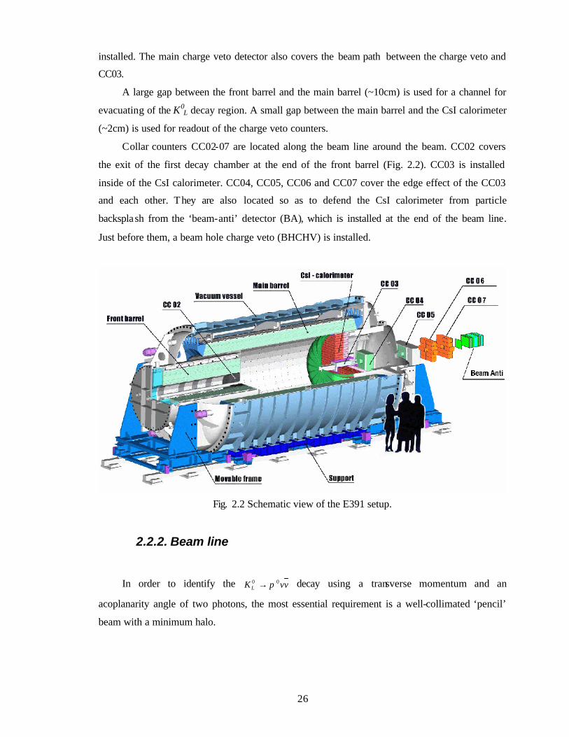
Collar counters CC02-07 are located along the beam line around the beam. CC02 covers

the exit of the first decay chamber at the end of the front barrel (Fig. 2.2). CC03 is installed

inside of the CsI calorimeter. CC04, CC05, CC06 and CC07 cover the edge effect of the CC03

and each other. They are also located so as to defend the CsI calorimeter from particle

backsplash from the ‘beam-anti’ detector (BA), which is installed at the end of the beam line.

Just before them, a beam hole charge veto (BHCHV) is installed.

Fig. 2.2 Schematic view of the E391 setup.

2.2.2. Beam line

In order to identify the vvKL00 π→ decay using a transverse momentum and an

acoplanarity angle of two photons, the most essential requirement is a well-collimated ‘pencil’

beam with a minimum halo.

27

A primary proton beam with a momentum of 13 GeV/c hits the K0L production target made

of platinum with 60 mm thickness and 8 mm diameter. The target is inclined by 4o horizontally

relative to the primary beam axis.

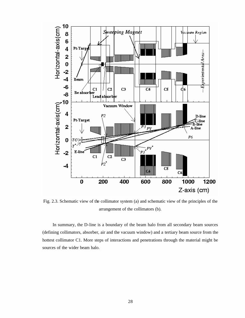
In Fig. 2.3(a), the beam collimator scheme is shown [41]. It consists of 6 collimators, a pair

of sweeping magnets, as well as Be and lead absorbers. The first three collimators (C1,C2,C3)

are used to define the beam profile with an aperture of 2 mrad in a half -cone angle. The last two

collimators (C5 and C6) are used to trim the beam halo. The lead and Be absorber is used to

reduce the γ and neutron fluxes relative to the K0L flux. Two dipole magnets are used for

sweeping out charged particles. The last collimator (C6) also acts as a sensitive detector to veto

the background events produced by a beam halo at that place. Because the length of the beam

line is about 10 m, hyperons in the neutral beam are reduced to a negligible level.

In Fig. 2.3 (b), the beam collimation scheme is presented by various lines:

• A-line is drawn as a line of the 2 mrad cone from the target center. The inner

surfaces of collimators C2 and C3 are placed along this line and define the core

profile of the beam.

• B-line is a line connecting T* and P3. C5 and the upstream-half of C6 are

arranged along this line. This line shows penumbra due to the finite size of the

target. The aperture of C5 and the upstream-half of C6 have a clearance of 0.2

mm with respect to the B-line. Then, the particles produced at the target do not

hit C5 and C6 directly.

• C-line connects P2* and P6. A lead absorber of 5 cm thick is placed between C1

and C2. Since its lateral size is small (1cm in diameter) and it is within the C-

line (extrapolated to the upstream direction), the free run-through of the

secondaries produced at the absorber is limited in the cone defined by this C-line.

• D-line is a line connecting PV* and P6. Since the upstream defining collimators

are enveloped in the D-line, it is a boundary for secondaries produced at the

defining collimators. It is also a boundary for the secondaries scattered by air

before the vacuum region and the window. The tertiaries originating from the

secondaries at C1 are also within this envelope, because the acceptance of the

secondaries from C1 is limited by the E-line. The latter half of C6 is arranged

along the D-line in order to prevent edge scatte ring of the particles from the

tertiaries mentioned above.

• E-line connects P2* and P3. The inner surface of C1 is arranged along this line.

Secondaries, which are produced at C1, should have a larger angle than the E-

line.

28

Fig. 2.3. Schematic view of the collimator system (a) and schematic view of the principles of the

arrangement of the collimators (b).

In summary, the D-line is a boundary of the beam halo from all secondary beam sources

(defining collimators, absorber, air and the vacuum window) and a tertiary beam source from the

hottest collimator C1. More steps of interactions and penetrations through the material might be

sources of the wider beam halo.

29

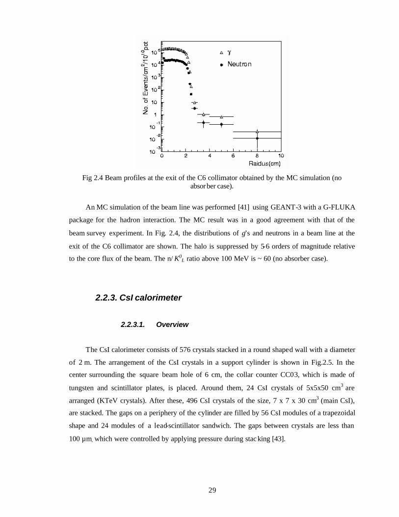
Fig 2.4 Beam profiles at the exit of the C6 collimator obtained by the MC simulation (no

absorber case).

An MC simulation of the beam line was performed [41] using GEANT-3 with a G-FLUKA

package for the hadron interaction. The MC result was in a good agreement with that of the

beam survey experiment. In Fig. 2.4, the distributions of γ’s and neutrons in a beam line at the

exit of the C6 collimator are shown. The halo is suppressed by 5-6 orders of magnitude relative

to the core flux of the beam. The n/ K0L ratio above 100 MeV is ~ 60 (no absorber case).

2.2.3. CsI calorimeter

2.2.3.1. Overview

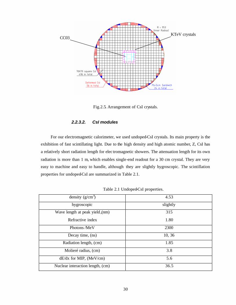
The CsI calorimeter consists of 576 crystals stacked in a round shaped wall with a diameter

of 2 m. The arrangement of the CsI crystals in a support cylinder is shown in Fig.2.5. In the

center surrounding the square beam hole of 6 cm, the collar counter CC03, which is made of

tungsten and scintillator plates, is placed. Around them, 24 CsI crystals of 5x5x50 cm3 are

arranged (KTeV crystals). After these, 496 CsI crystals of the size, 7 x 7 x 30 cm3 (main CsI),

are stacked. The gaps on a periphery of the cylinder are filled by 56 CsI modules of a trapezoidal

shape and 24 modules of a lead-scintillator sandwich. The gaps between crystals are less than

100 µm, which were controlled by applying pressure during stac king [43].

30

Fig.2.5. Arrangement of CsI crystals.

2.2.3.2. CsI modules

For our electromagnetic calorimeter, we used undoped-CsI crystals. Its main property is the

exhibition of fast scintillating light. Due to the high density and high atomic number, Z, CsI has

a relatively short radiation length for elec tromagnetic showers. The attenuation length for its own

radiation is more than 1 m, which enables single-end readout for a 30 cm crystal. They are very

easy to machine and easy to handle, although they are slightly hygroscopic. The scintillation

properties for undoped-CsI are summarized in Table 2.1.

Table 2.1 Undoped-CsI properties.

density (g/cm3) 4.53

hygroscopic slightly

Wave length at peak yield ,(nm) 315

Refractive index 1.80

Photons /MeV 2300

Decay time, (ns) 10, 36

Radiation length, (cm) 1.85

Molieré radius, (cm) 3.8

dE/dx for MIP, (MeV/cm) 5.6

Nuclear interaction length, (cm) 36.5

KTeV crystals CC03

31

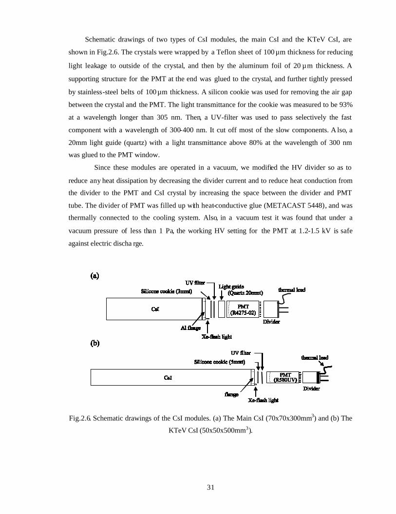
Schematic drawings of two types of CsI modules, the main CsI and the KTeV CsI, are

shown in Fig.2.6. The crystals were wrapped by a Teflon sheet of 100 µm thickness for reducing

light leakage to outside of the crystal, and then by the aluminum foil of 20 µm thickness. A

supporting structure for the PMT at the end was glued to the crystal, and further tightly pressed

by stainless-steel belts of 100 µm thickness. A silicon cookie was used for removing the air gap

between the crystal and the PMT. The light transmittance for the cookie was measured to be 93%

at a wavelength longer than 305 nm. Then, a UV-filter was used to pass selectively the fast

component with a wavelength of 300-400 nm. It cut off most of the slow components. A lso, a

20mm light guide (quartz) with a light transmittance above 80% at the wavelength of 300 nm

was glued to the PMT window.

Since these modules are operated in a vacuum, we modified the HV divider so as to

reduce any heat dissipation by decreasing the divider current and to reduce heat conduction from

the divider to the PMT and CsI crystal by increasing the space between the divider and PMT

tube. The divider of PMT was filled up with heat-conductive glue (METACAST 5448), and was

thermally connected to the cooling system. Also, in a vacuum test it was found that under a

vacuum pressure of less than 1 Pa, the working HV setting for the PMT at 1.2-1.5 kV is safe

against electric discha rge.

Fig.2.6. Schematic drawings of the CsI modules. (a) The Main CsI (70x70x300mm3) and (b) The

KTeV CsI (50x50x500mm3).

32

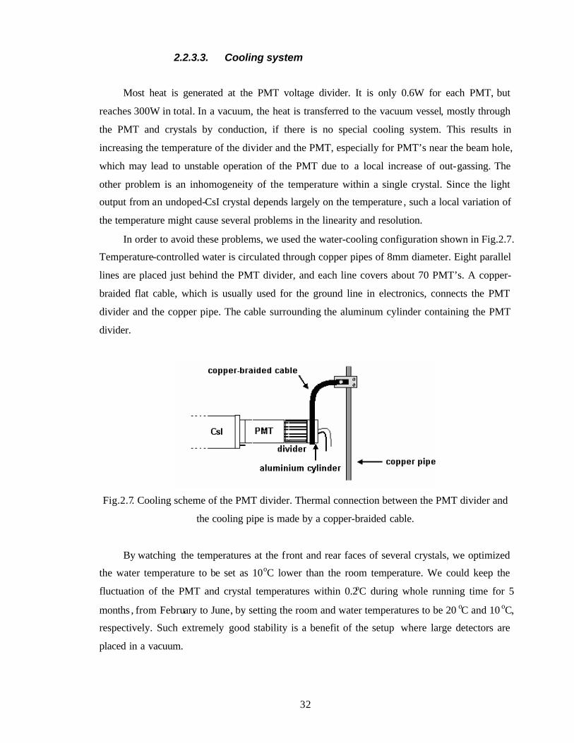
2.2.3.3. Cooling system

Most heat is generated at the PMT voltage divider. It is only 0.6W for each PMT, but

reaches 300W in total. In a vacuum, the heat is transferred to the vacuum vessel, mostly through

the PMT and crystals by conduction, if there is no special cooling system. This results in

increasing the temperature of the divider and the PMT, especially for PMT’s near the beam hole,

which may lead to unstable operation of the PMT due to a local increase of out-gassing. The

other problem is an inhomogeneity of the temperature within a single crystal. Since the light

output from an undoped-CsI crystal depends largely on the temperature , such a local variation of

the temperature might cause several problems in the linearity and resolution.

In order to avoid these problems, we used the water-cooling configuration shown in Fig.2.7.

Temperature-controlled water is circulated through copper pipes of 8mm diameter. Eight parallel

lines are placed just behind the PMT divider, and each line covers about 70 PMT’s. A copper-

braided flat cable, which is usually used for the ground line in electronics, connects the PMT

divider and the copper pipe. The cable surrounding the aluminum cylinder containing the PMT

divider.

Fig.2.7. Cooling scheme of the PMT divider. Thermal connection between the PMT divider and

the cooling pipe is made by a copper-braided cable.

By watching the temperatures at the front and rear faces of several crystals, we optimized

the water temperature to be set as 10oC lower than the room temperature. We could keep the

fluctuation of the PMT and crystal temperatures within 0.2oC during whole running time for 5

months , from February to June, by setting the room and water temperatures to be 20 oC and 10 oC,

respectively. Such extremely good stability is a benefit of the setup where large detectors are

placed in a vacuum.

33

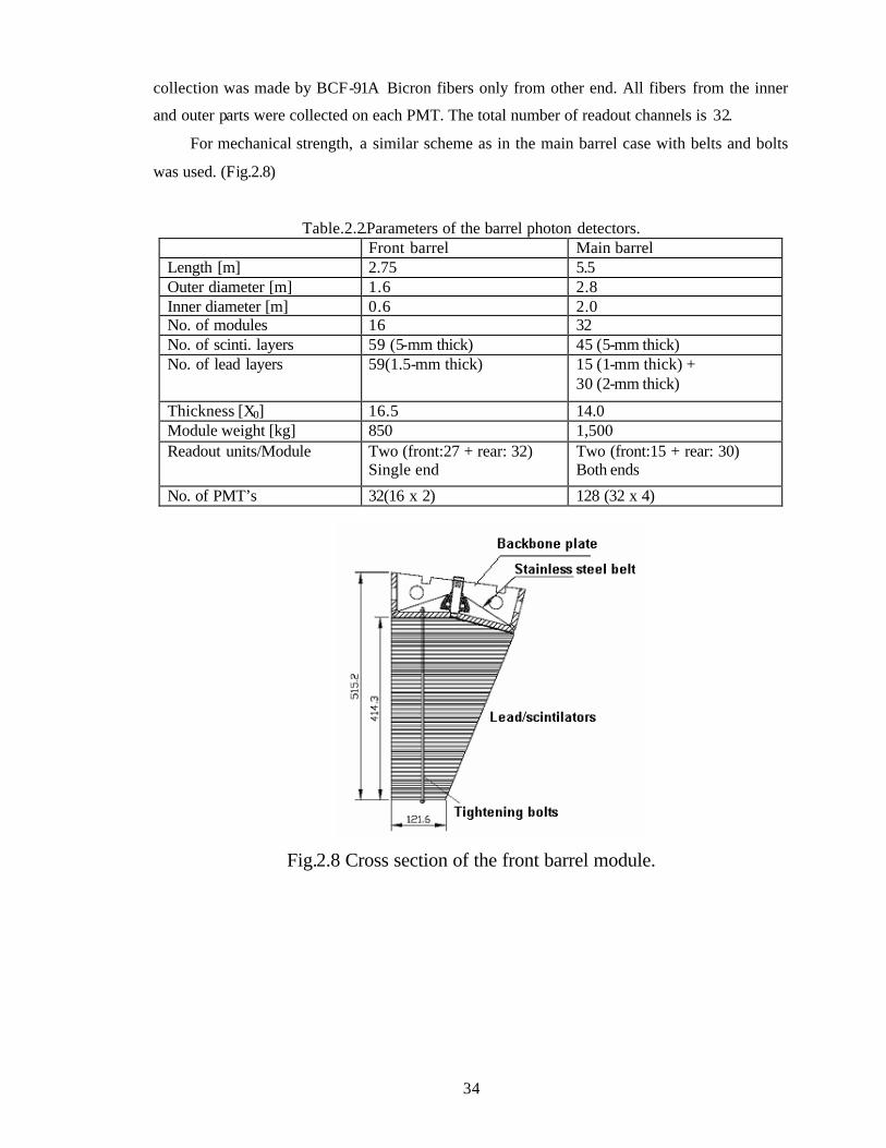
2.2.4. Main and front barrels

2.2.4.1. Main barrel

The main barrel modules of about 550cm length are lead/scintillator sandwiches with

wavelength shifter fiber readout form both ends. The readout layers are separated into two parts:

the inner part with 16 lead plates with 1mm thickness, and the outer part with 29 lead plates with

2mm thickness. The thickness of the scintillator is 5 mm. The scintillation light is collected by

wavelength shifter fibers (KURARAY-Y11-M). For reducing the light loss, reflector sheets of

TiO2PET with a thickness of 188 µm were inserted between the lead and scintillator layers. All

fibers from each layer were collected to one PMT, so that each module had 4 PMT’s. In total, we

had 128 readout channels.

For mechanical strength of the module, a thick stainless-steel plate was used as a backbone

structure. The scintillators and lead sheets were tightened to the backbone plate by 50 bolts of 5

mm diameter passing through holes in the scintillator and lead plates over the 550 cm length. A 3

mm-thick steel plate was placed at the opposite side of the backbone plate to fix the nuts , as

shown in Fig.2.9.

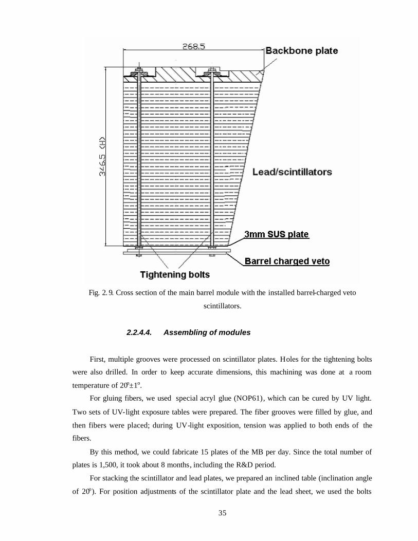
2.2.4.2. Barrel charge veto

A barrel charge veto detector was installed on the inner surface of MBR, as shown in Fig

2.9. Two scintillator sheets of 5mm each were glued to each other with a small shift to cover the

gap between the modules. The ends of the bolts of the main barrel modules were used for fixing

the scintillators on the inner surface of the main barrel. A reflector sheet of TiO2PET was glued

over the scintillator to reduce any light leakage. Fibers at each side were connected to a 1-inch

PMT. The total number of readout channels is 64.

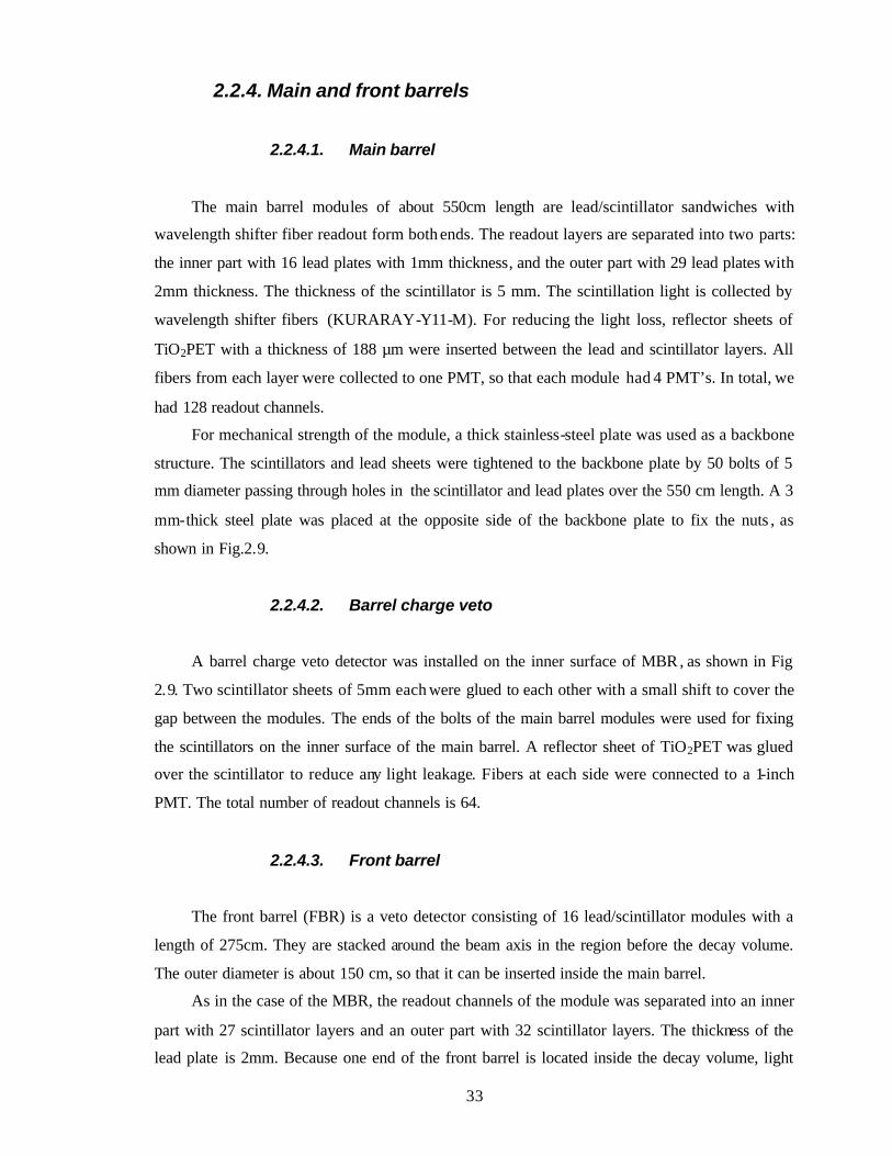
2.2.4.3. Front barrel

The front barrel (FBR) is a veto detector consisting of 16 lead/scintillator modules with a

length of 275cm. They are stacked around the beam axis in the region before the decay volume.

The outer diameter is about 150 cm, so that it can be inserted inside the main barrel.

As in the case of the MBR, the readout channels of the module was separated into an inner

part with 27 scintillator layers and an outer part with 32 scintillator layers. The thickness of the

lead plate is 2mm. Because one end of the front barrel is located inside the decay volume, light

34

collection was made by BCF-91A Bicron fibers only from other end. All fibers from the inner

and outer parts were collected on each PMT. The total number of readout channels is 32.

For mechanical strength, a similar scheme as in the main barrel case with belts and bolts

was used. (Fig.2.8)

Table.2.2.Parameters of the barrel photon detectors. Front barrel Main barrel Length [m] 2.75 5.5 Outer diameter [m] 1.6 2.8 Inner diameter [m] 0.6 2.0 No. of modules 16 32 No. of scinti. layers 59 (5-mm thick) 45 (5-mm thick) No. of lead layers 59(1.5-mm thick)

15 (1-mm thick) + 30 (2-mm thick)

Thickness [X0] 16.5 14.0 Module weight [kg] 850 1,500 Readout units/Module Two (front:27 + rear: 32)

Single end Two (front:15 + rear: 30) Both ends

No. of PMT’s 32(16 x 2) 128 (32 x 4)

Fig.2.8 Cross section of the front barrel module.

35

Fig. 2. 9. Cross section of the main barrel module with the installed barrel-charged veto

scintillators.

2.2.4.4. Assembling of modules

First, multiple grooves were processed on scintillator plates. Holes for the tightening bolts

were also drilled. In order to keep accurate dimensions, this machining was done at a room

temperature of 20o±1o.

For gluing fibers, we used special acryl glue (NOP61), which can be cured by UV light.

Two sets of UV-light exposure tables were prepared. The fiber grooves were filled by glue, and

then fibers were placed; during UV-light exposition, tension was applied to both ends of the

fibers.

By this method, we could fabricate 15 plates of the MB per day. Since the total number of

plates is 1,500, it took about 8 months, including the R&D period.

For stacking the scintillator and lead plates, we prepared an inclined table (inclination angle

of 20o). For position adjustments of the scintillator plate and the lead sheet, we used the bolts

36

passing through the module. Since the length of the lead sheet is limited to be less than 1.5 m for

easy handling, we used four separate sheets for the MBR and two for the FBR. Between the

scintillator plate and the lead sheet, we inserted a reflector sheet of TiO2PET. After stacking a

half layer of the laminate, we applied a pressure of 3 tons/m from the backside by a press. By

doing this press, lead sheets were flattened and the thickness of the module could be checked

during the stacking process. Inaccuracies of the thickness resulted from thickness variations of

the lead sheets.

After stacking all lead and scintillator plates, we attached the backbone plate and applied

a pressure of about 3 tons/m for at least 12 hours. Under the pressed condition, we attached five

steel belts and six stud bolts for the FBR, and 50 stud bolts for the MBR. After adjusting the

torque for each nut, we released the pressure that had been applied by the press.

Light readout was made from a single end in the case of the FBR and from both ends in the

case of the MBR. These fibers were bundled at the end, and fixed to a plastic holder with glue.

We then cut the fiber bundle together with the plastic holder with a diamond cutter to make a flat

contact surface. For a good optical transmission of light, we polished the cut surface with

polishing powders. PMT’s were attached to the flat surface through silicone rubber of 3 mm-

thick.

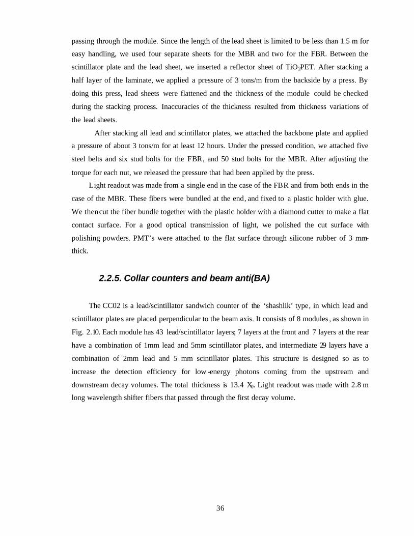
2.2.5. Collar counters and beam anti(BA)

The CC02 is a lead/scintillator sandwich counter of the ‘shashlik’ type, in which lead and

scintillator plate s are placed perpendicular to the beam axis. It consists of 8 modules , as shown in

Fig. 2.10. Each module has 43 lead/scintillator layers; 7 layers at the front and 7 layers at the rear

have a combination of 1mm lead and 5mm scintillator plates, and intermediate 29 layers have a

combination of 2mm lead and 5 mm scintillator plates. This structure is designed so as to

increase the detection efficiency for low -energy photons coming from the upstream and

downstream decay volumes. The total thickness is 13.4 X0. Light readout was made with 2.8 m

long wavelength shifter fibers that passed through the first decay volume.

37

Fig. 2.10 CC02 schematic view. The CC02 counter is installed inside the front barrel.

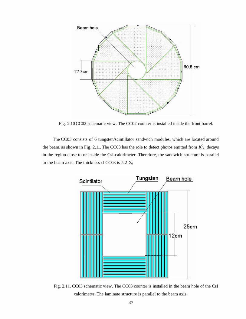
The CC03 consists of 6 tungsten/scintillator sandwich modules, which are located around

the beam, as shown in Fig. 2.11. The CC03 has the role to detect photos emitted from K0L decays

in the region close to or inside the CsI calorimeter. Therefore, the sandwich structure is parallel

to the beam axis. The thickness of CC03 is 5.2 X0

Fig. 2.11. CC03 schematic view. The CC03 counter is installed in the beam hole of the CsI

calorimeter. The laminate structure is parallel to the beam axis.

38

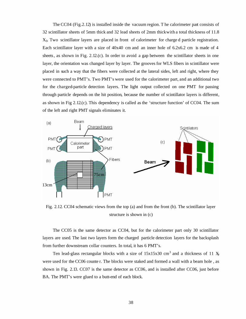
The CC04 (Fig.2.12) is installed inside the vacuum region. T he calorimeter part consists of

32 scintillator sheets of 5mm thick and 32 lead sheets of 2mm thick with a total thickness of 11.8

X0. Two scintillator layers are placed in front of calorimeter for charge d particle registration.

Each scintillator layer with a size of 40x40 cm and an inner hole of 6.2x6.2 cm is made of 4

sheets , as shown in Fig. 2.12.(c). In order to avoid a gap between the scintillator sheets in one

layer, the orientation was changed layer by layer. The grooves for WLS fibers in scintillator were

placed in such a way that the fibers were collected at the lateral sides, left and right, where they

were connected to PMT’s. Two PMT’s were used for the calorimeter part, and an additional two

for the charged-particle detection layers. The light output collected on one PMT for passing

through particle depends on the hit position, because the number of scintillator layers is different,

as shown in Fig 2.12.(c). This dependency is called as the ‘structure function’ of CC04. The sum

of the left and right PMT signals eliminates it.

Fig. 2.12. CC04 schematic views from the top (a) and from the front (b). The scintillator layer

structure is shown in (c)

The CC05 is the same detector as CC04, but for the calorimeter part only 30 scintillator

layers are used. The last two layers form the charged particle detection layers for the backsplash

from further downstream collar counters. In total, it has 6 PMT’s.

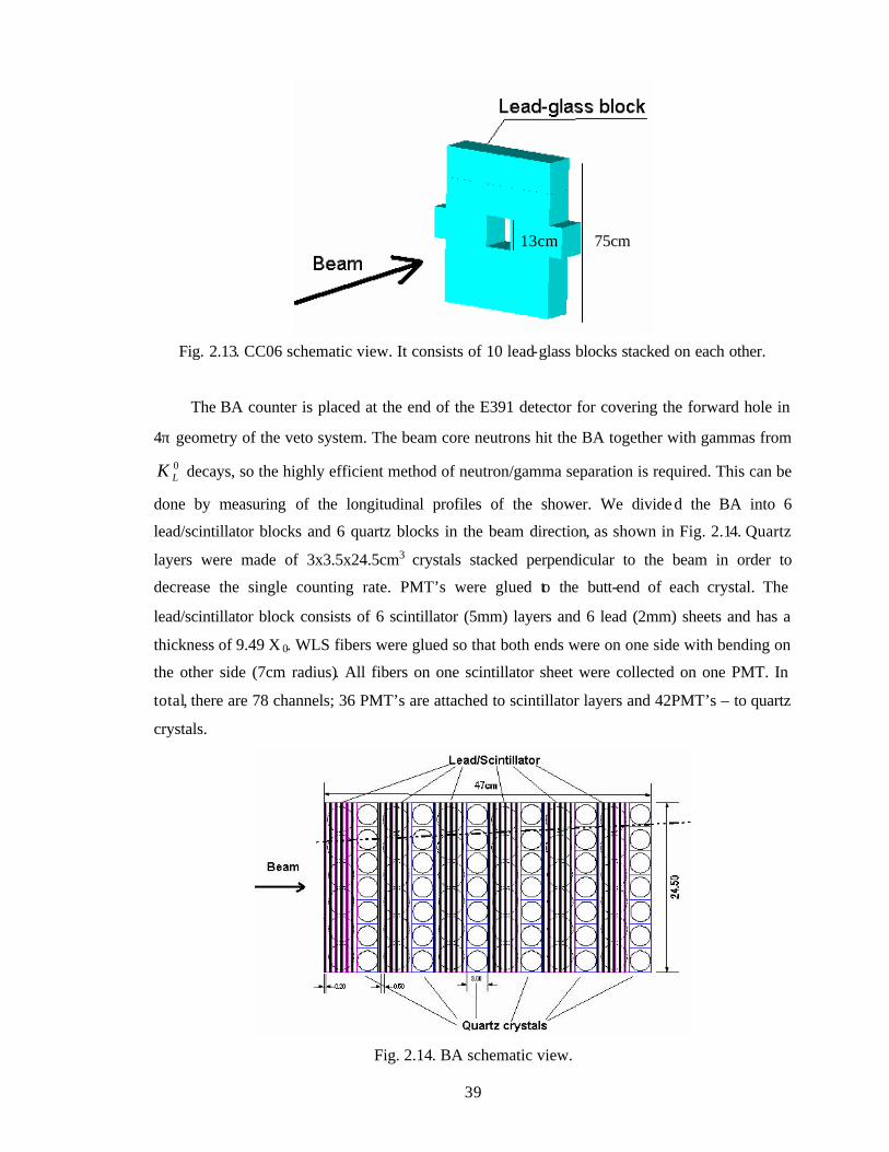
Ten lead-glass rectangular blocks with a size of 15x15x30 cm3 and a thickness of 11 X0

were used for the CC06 counte r. The blocks were staked and formed a wall with a beam hole , as

shown in Fig. 2.13. CC07 is the same detector as CC06, and is installed after CC06, just before

BA. The PMT’s were glued to a butt-end of each block.

75cm

13cm

39

Fig. 2.13. CC06 schematic view. It consists of 10 lead-glass blocks stacked on each other.

The BA counter is placed at the end of the E391 detector for covering the forward hole in

4π geometry of the veto system. The beam core neutrons hit the BA together with gammas from

0LK decays, so the highly efficient method of neutron/gamma separation is required. This can be

done by measuring of the longitudinal profiles of the shower. We divide d the BA into 6

lead/scintillator blocks and 6 quartz blocks in the beam direction, as shown in Fig. 2.14. Quartz

layers were made of 3x3.5x24.5cm3 crystals stacked perpendicular to the beam in order to

decrease the single counting rate. PMT’s were glued to the butt-end of each crystal. The

lead/scintillator block consists of 6 scintillator (5mm) layers and 6 lead (2mm) sheets and has a

thickness of 9.49 X 0. WLS fibers were glued so that both ends were on one side with bending on

the other side (7cm radius). All fibers on one scintillator sheet were collected on one PMT. In

total, there are 78 channels; 36 PMT’s are attached to scintillator layers and 42PMT’s – to quartz

crystals.

Fig. 2.14. BA schematic view.

75cm 13cm

40

2.2.6. Vacuum system

2.2.6.1. Overview

For the vvKL00 π→ decay, a very high vacuum along the beam path is required to reduce

the background due to interactions of the beam with residual gas. For our experimental setup, an

estimation of the background has already been done [41]. Background events of 0.08 (G-

FLUKA), 0.01 (G-CALOR) and 0.006 (GHEISHA) are predicted at a vacuum pressure of 10-5

Pa for a sensitivity of 3x10-11 for the vvKL00 π→ decay. Therefore, in the case of E391a, whose

sensitivity is 3x10-10, a vacuum of higher than 10-4 Pa is required in order to reduce the

background down to a negligible level (< 0.1 events), even for the worst case predicted by G-

FLUKA. On the other hand, an experiment for vvKL00 π→ decay requires highly sensitive

detection for particles in order to reduce the backgrounds from other decay modes and from

interactions of the halo neutrons.

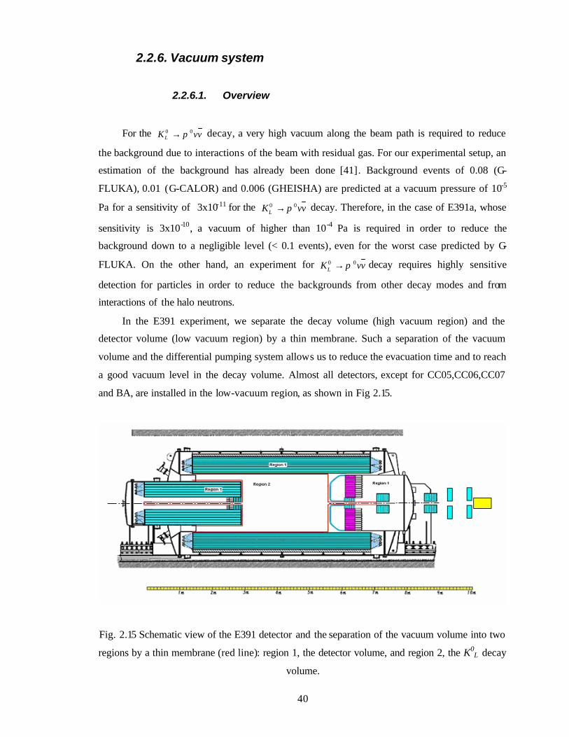
In the E391 experiment, we separate the decay volume (high vacuum region) and the

detector volume (low vacuum region) by a thin membrane. Such a separation of the vacuum

volume and the differential pumping system allows us to reduce the evacuation time and to reach

a good vacuum level in the decay volume. Almost all detectors, except for CC05,CC06,CC07

and BA, are installed in the low-vacuum region, as shown in Fig 2.15.

Fig. 2.15 Schematic view of the E391 detector and the separation of the vacuum volume into two

regions by a thin membrane (red line): region 1, the detector volume, and region 2, the K0L decay

volume.

41

2.2.6.2. Scheme of pumping

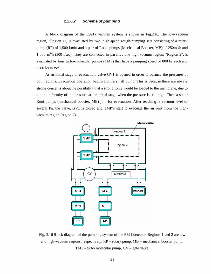
A block diagram of the E391a vacuum system is shown in Fig.2.16. The low-vacuum

region, “Region 1”, is evacuated by two high-speed rough-pumping sets consisting of a rotary

pump (RP) of 1,500 l/min and a pair of Roots pumps (Mechanical Booster, MB) of 250m3/h and

1,000 m3/h (300 l/sec). They are connected in parallel. The high-vacuum region, “Region 2”, is

evacuated by four turbo-molecular pumps (TMP) that have a pumping speed of 800 l/s each and

3200 l/s in total.

At an initial stage of evacuation, valve GV1 is opened in order to balance the pressures of

both regions. Evacuation operation begins from a small pump. This is because there are always

strong concerns about the possibility that a strong force would be loaded to the membrane, due to

a non-uniformity of the pressure at the initial stage when the pressure is still high. Then a set of

Root pumps (mechanical booster, MB) join for evacuation. After reaching a vacuum level of

several Pa, the valve, GV1 is closed and TMP’s start to evacuate the air only from the high-

vacuum region (region 2).

.

Fig. 2.16 Block diagram of the pumping system of the E391 detector. Regions 1 and 2 are low

and high-vacuum regions, respectively. RP – rotary pump, MB – mechanical booster pump,

TMP –turbo molecular pump, GV – gate valve.

42

2.2.6.3. Bench tests of the membrane

To separate the low and high-vacuum regions, a plastic sheet, called EVON, was chosen. It

is a lamination of 80 µm low-density polyethylene, 15 µm aluminized EVAL film, 15 µm nylon

and 80 µm low-density polyethylene. It is ordinarily used for an airship, which is required to be

mechanically very strong. The total thickness of the sheet is 20 mg/cm2.

Through a bench test, it was found that the outgassing rate is 9x10-6 Pa m3 / (sec m2 ) at

room temperature after 167.7 hours of evacuation. It was also observed that a kind of baking

effect decreased the outgassing rate to 4.2x10-8 Pa m3 / (sec m2) after a heat-up to 50 degrees.

The main component of the out-gas, which was analyzed by a mass separator, was water vapor.

According to their catalogue , transmission of gas through EVON is 1, 0.030, <0.1 and <0.01

cc/m2 /24 hours for He, O2, CO2 and N2 gas, respectively. These values are far below the

required level for the E391 vacuum.

Another merit of this material is that sheets can be easily jointed with each other by

applying heat to the low-density polyethylene layers on both sides.

43

Chapter 3

Data taking in a physics run

3.1 DAQ system

3.1.1 Overview

A distributed and parallel processing DAQ system has been developed for the E391a

experiment. Data from front-end FASTBUS-ADC’s and TKO-TDC’s are read out by VME

board computers , and sent to the server computer via a network.

The E391 detector consists of electromagnetic calorimeter and veto counters covering full

4 π geometry. All of these detectors use photomultipliers (PMT) for light readout. Table 4.1 lists

the number of channels of each detector subsystem. Both the charge and the timing of each PMT

signal are measured by the DAQ system. These signals are also used for online triggering. The

total number of readout channe ls is about 1000.

44

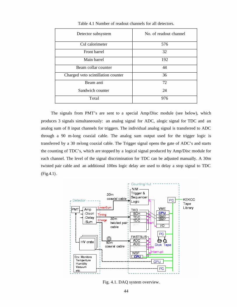
Table 4.1 Number of readout channels for all detectors.

Detector subsystem No. of readout channel

CsI calorimeter 576

Front barrel 32

Main barrel 192

Beam collar counter 44

Charged veto scintillation counter 36

Beam anti 72

Sandwich counter 24

Total 976

The signals from PMT’s are sent to a special Amp/Disc module (see below), which

produces 3 signals simultaneously: an analog signal for ADC, alogic signal for TDC and an

analog sum of 8 input channels for triggers. The individual analog signal is transferred to ADC

through a 90 m-long coaxial cable. The analog sum output used for the trigger logic is

transferred by a 30 m-long coaxial cable. The Trigger signal opens the gate of ADC’s and starts

the counting of TDC’s, which are stopped by a logical signal produced by Amp/Disc module for

each channel. The level of the signal discrimination for TDC can be adjusted manually. A 30m

twisted pair cable and an additional 100ns logic delay are used to delay a stop signal to TDC

(Fig.4.1) .

Fig. 4.1. DAQ system overview.

45

The HV power supplies are installed in the beam area near to the detectors. We used 7

CAEN SY527 crates which have a remote control system, and allow us to board up 10 modules.

Modules (A737N) having 16 channels with an output HV of up to 3kV were used.

Various environmental parameters, the temperature, the vacuum level and so on are

monitored. Information from them is saved to the disk for the further analysis.

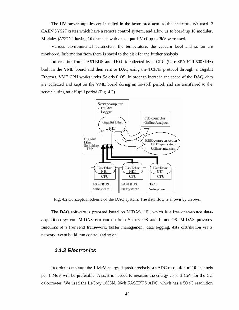
Information from FASTBUS and TKO is collected by a CPU (UltraSPARCII 500MHz)

built in the VME board, and then sent to DAQ using the TCP/IP protocol through a Gigabit

Ethernet. VME CPU works under Solaris 8 OS. In order to increase the speed of the DAQ, data

are collected and kept on the VME board during an on-spill period, and are transferred to the

server during an off-spill period (Fig. 4.2)

Fig. 4.2 Conceptual scheme of the DAQ system. The data flow is shown by arrows.

The DAQ software is prepared based on MIDAS [10], which is a free open-source data-

acquis ition system. MIDAS can run on both Solaris OS and Linux OS. MIDAS provides

functions of a front-end framework, buffer management, data logging, data distribution via a

network, event build, run control and so on.

3.1.2 Electronics

In order to measure the 1 MeV energy deposit precisely, an ADC resolution of 10 channels

per 1 MeV will be preferable. Also, it is needed to measure the energy up to 3 GeV for the CsI

calorimeter. We used the LeCroy 1885N, 96ch FASTBUS ADC, which has a 50 fC resolution

46

per channel. The charge conversion time is 750 µsec , which restricts the speed of data

acquisition up to 1000 Hz, at most.

In order to reduce accidental background events, 1 nsec of the event-timing resolution is

required. In some cases, we also have to distinguish the incident angle of γ to the CsI calorimeter

for a further reduction of the background. For that purpose, less than 0.1 nsec of the timing

resolution is necessary. We decided to use 64ch TKO-TDC as a TDC module. The resolution is

0.05 nsec. The TDC is operated in the common-start and individual-stop mode.

Multihit TDC is useful in some cases. BA suffers from a huge counting rate due to the

neutral beam. We need to separate the γ’s from K0 decays and γ’s and neutrons in the beam. We

have chosen the LeCroy 1877S FASTBUS TDC. It has 96 channels in a module, and each

channel has a 16 bit depth of the buffer. Because dynamic range is 32 µsec, the resolution is 0.5

nsec The data-conversion time is less than 80 µsec.

3.1.3 Trigger logic

The global trigger logic accepts multiple trigger signals simultaneously from multiple

subsystems: a random trigger from the clock generator, a cosmic event trigger from MBR, a

Xenon/LED flush, number-of-CsI-cluster (N cluster) trigger from the cluster counting logic,

accidental triggers and so on. A trigger decision is made within 200 nsec after a trigger request.

During the data collection time, the next trigger requests and a flash of the xenon lamp are

suppressed.

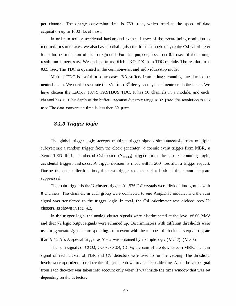
The main trigger is the N-cluster trigger. All 576 CsI crystals were divided into groups with

8 channels. The channels in each group were connected to one Amp/Disc module , and the sum

signal was transferred to the trigger logic. In total, the CsI calorimeter was divided onto 72

clusters, as shown in Fig. 4.3.

In the trigger logic, the analog cluster signals were discriminated at the level of 60 MeV

and then 72 logic output signals were summed up. Discriminators with different thresholds were

used to generate signals corresponding to an event with the number of hit-clusters equal or grate

than N ( N≥ ). A special trigger as N = 2 was obtained by a simple logic )3()2( ≥⋅≥ NN .

The sum signals of CC02, CC03, CC04, CC05; the sum of the downstream MBR, the sum

signal of each cluster of FBR and CV detectors were used for online vetoing. The threshold

levels were optimized to reduce the trigger rate down to an acceptable rate. Also, the veto signal

from each detector was taken into account only when it was inside the time window that was set

depending on the detector.

47

Fig. 4.3 Scheme of the CsI cluster layout.

3.1.4 Server computer and network

The server computer is a PC with a Linux OS. Data from each detector are collected on the

server and built by using MIDAS builder software , and are saved on the hard disk of the server

(Fig. 4.2). Online analysis is performed by a sub-computer using a part of the built data sent via

the network. The stored data are sent to a tape library in the KEK central computer-system in

order to perform an offline analysis. The VME computer has a network interface (NIC) for the

Fast Ethernet.

Although the network speed is sufficient to send data from each subsystem, the total traffic

with sending data to the tape library is huge. Therefore we adopted a NIC of Giga-Bit Ethernet

on the server computer. The server computer and subsystems are connected with a switching hub,

which is used for both the Fast and Giga-bit Ethernet.

3.1.5 DAQ performance

The beam from KEK-PS comes in a 4-second cycle and the beam duration is about 2

seconds. The subsystem stores data during a beam spill, and sends the stored data when the beam

48

is off. The dead time for one-event data taking is 1800 secµ for FASTBUS and 420 secµ for

TKO

The DAQ was tested in an Engineering run in Oct.-Dec. in 2002. At that time, not all of the

detectors were ready. However, our main detector, the CsI calorimeter that has the largest

number of channels, had been prepared for the engineering run. The proton-beam intensity was

about 1012 per spill and the trigger rate was less than 200 Hz. In a physics run in 2004, the

FASTBUS ADC’s were upgraded in terms of reducing the dead time. We reached a dead time of

1000 secµ which allowed us to increase the trigger rate up to about 500 Hz during the physics

run.

3.2 Data taking in 2004 physics runs

In February 15, we started physics data taking. The beam run continued until June 30. The

first two weeks were used for beam tuning, DAQ tuning and detector calibration by the muon

beam. At the end of the data taking, 15 shifts were used for calibration of the CsI calorimeter by

π 0‘s produced on a target. In total, we had 175 shifts of physics data taking. The duration of the

shift is 8 hours.

3.2.1 Triggers during physics data taking

o Physics trigger

During physics data taking, we collected data with various triggers simultaneously. The

main trigger was ≥clusterN 2 + veto. Our goal was to collect as many 2γ events as possible.

Furthermore, data from other decay modes , such as 00 3π→LK and 00 2π→LK , were needed to

monitor the number of 0LK ’s coming to the E391 setup. Thus, this trigger mode allowed us to

collect data for all 0LK decays with the number of γ‘s more than or equal to 2.

The online veto thresholds were optimized so as reduce background events , and not to lose

real events. In order to reduce the acceptance loss due to accidental hits, the time windows of the

veto signals were set in the trigger logic.

o Monitor triggers

In order to monitor accidental events, three special triggers were prepared. They were the

signal of TMON, a counter telescope near the K0 production target used to monitor the targeting

efficiency; the signal of C6, located at the exit of the beam line; and the signal from BA.

49

The pedestal events triggered by a clock and the Xenon/LED events triggered by a signal to

the flash Xenon lamp and LED were used to monitor the drift of the system during data taking.

These triggers were fired in both the beam-on and off periods in order to check the beam-loading

effects.

o Minimum bias triggers

To study the veto inefficiency, a minimum bias trigger was also prepared. It was ≥clusterN 1

without any veto. An additional one was ≥clusterN 2 without any veto, which was useful to study

the veto inefficiency with the same trigger condition as the main physics trigger.

o Triggers for calibration

Additional triggers were a cosmic trigger, a coincidence of the opposite main barrel

clusters; and a muon trigger , a coincidence of the CC04 and CC05 beam collar counters. The

comic trigger was fired only in the beam-off time. The muon trigger was used to calibrate the

beam counter, and during physics data taking, for monitoring their gain constants.

3.2.2 Data taking

o Physics data

We collected about 6Tb data by the physics trigger ≥clusterN 2 + veto. The main trigger

allowed us to collect data of various K0 decay modes. The 00 3π→LK decay is very clean in

terms of the background, and can be used for a detailed comparison of the data and the MC

simulation results. The 00 2π→LK and γγ→0LK decays can be used to monitor the number of

K0‘s coming to the E391 setup.

o Special runs for the detector calibration

For detector calibration, we performed special runs using the muon beam by closing the C3

collimator. For CsI calibration, the trigger was clusterN =1 without any veto. The collar counters

were calibrated using the coincidence of the CC04 and CC05 as a trigger. The data for the BA

calibration was taken by a self-trigger. Special runs using cosmic rays were performed to

calibrate the CsI calorimeter during a beam break.

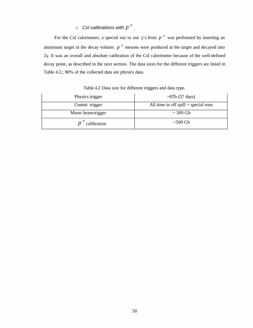
50

o CsI calibrations with 0π .

For the CsI calorimeter, a special run to use γ’s from 0π was performed by inserting an

aluminum target in the decay volume. 0π mesons were produced at the target and decayed into

2γ. It was an overall and absolute calibration of the CsI calorimeter because of the well-defined

decay point, as described in the next section. The data sizes for the different triggers are listed in

Table 4.2.; 80% of the collected data are physics data.

Table 4.2 Data size for different triggers and data type.

Physics trigger ~6Tb (57 days)

Cosmic trigger All time in off spill + special runs

Muon beam trigger ~ 300 Gb

0π calibration ~500 Gb

51

Chapter 4

Calibration of the detectors

4.1 Pedestals

In order to monitor the stability of the electronics system, we measured the ADC pedestals

with a 1Hz frequency in the physics run. Our ADC’s work in two modes: a high-gain mode (0.05

pC/ch) and a low-gain mode (0.4 pC/ch). The pedestals in both modes were periodically

measured during the beam-off and the beam-on periods.

In Fig. 4.1, typical distributions of the pedestals for all detectors (high-gain mode) in the

beam-on period are presented. All of the detectors, except for the sandwich counters (see below),

have small pedestal fluctuations (σ) of about 1.5 channels (high-gain mode) and about 1 channel

(low -gain mode). The pedestals of some detectors suffer from accidental hits, but there is no

meaningful difference between the peak position of the pedestals in on-spill data and that in off-

spill data. In Fig. 4.2, the distributions of the pedestal width (σ) for the high and low-gain modes

for all CsI crystals are shown. All other detectors, except the sandwich counters , have the same

width of pedestals.

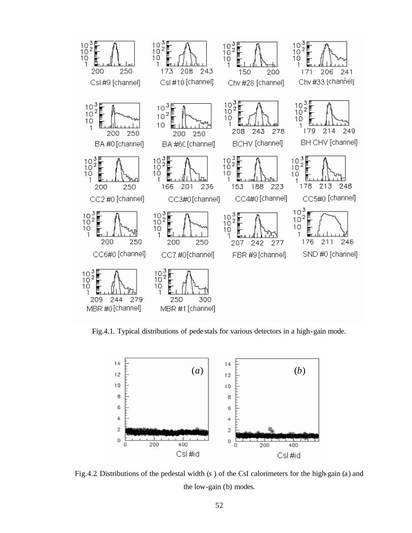
52

Fig.4.1. Typical distributions of pedestals for various detectors in a high-gain mode.

Fig.4.2. Distributions of the pedestal width (σ) of the CsI calorimeters for the high-gain (a) and

the low-gain (b) modes.

)(a )(b

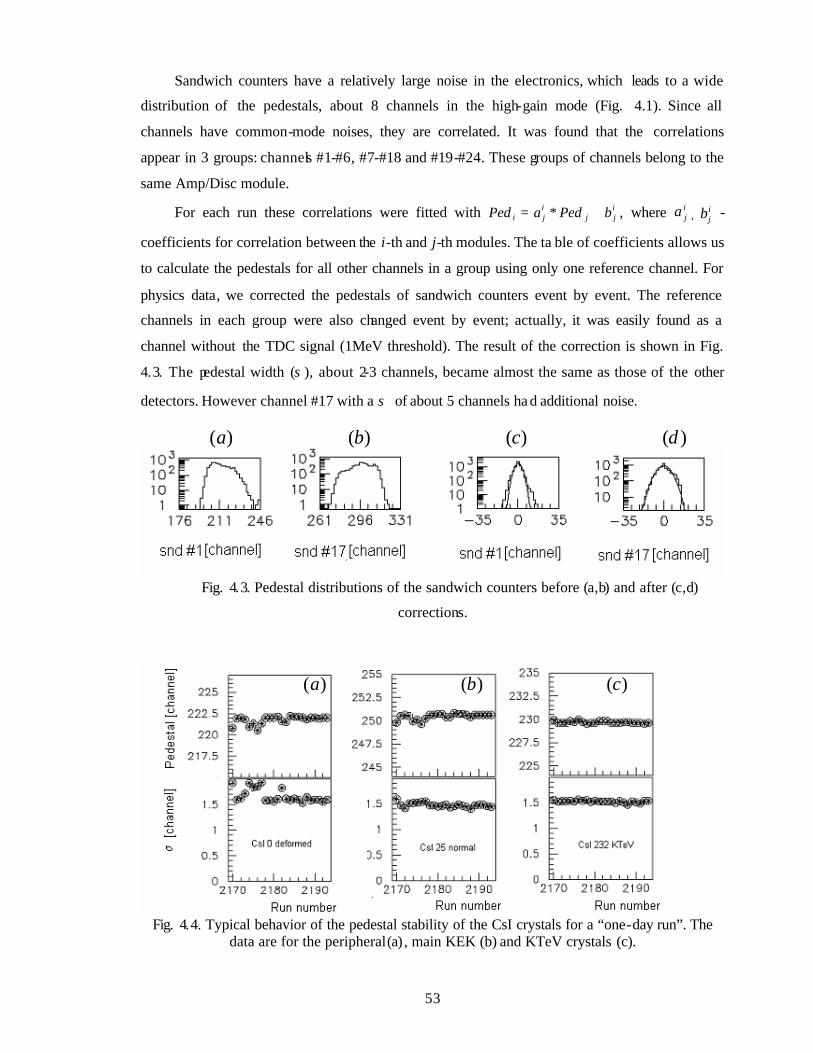
53

Sandwich counters have a relatively large noise in the electronics, which leads to a wide

distribution of the pedestals, about 8 channels in the high-gain mode (Fig. 4.1). Since all

channels have common-mode noises, they are correlated. It was found that the correlations

appear in 3 groups: channels #1-#6, #7-#18 and #19-#24. These groups of channels belong to the

same Amp/Disc module.

For each run these correlations were fitted with ijj

iji bPedaPed += * , where i

ja , ijb -

coefficients for correlation between the i-th and j-th modules. The ta ble of coefficients allows us

to calculate the pedestals for all other channels in a group using only one reference channel. For

physics data, we corrected the pedestals of sandwich counters event by event. The reference

channels in each group were also changed event by event; actually, it was easily found as a

channel without the TDC signal (1MeV threshold). The result of the correction is shown in Fig.

4.3. The pedestal width (σ), about 2-3 channels, became almost the same as those of the other

detectors. However channel #17 with a σ of about 5 channels ha d additional noise.

Fig. 4.3. Pedestal distributions of the sandwich counters before (a,b) and after (c,d)

corrections.

Fig. 4.4. Typical behavior of the pedestal stability of the CsI crystals for a “one-day run”. The

data are for the peripheral (a) , main KEK (b) and KTeV crystals (c).

)(c )(d

)(a )(b

)(a )(b

)(c

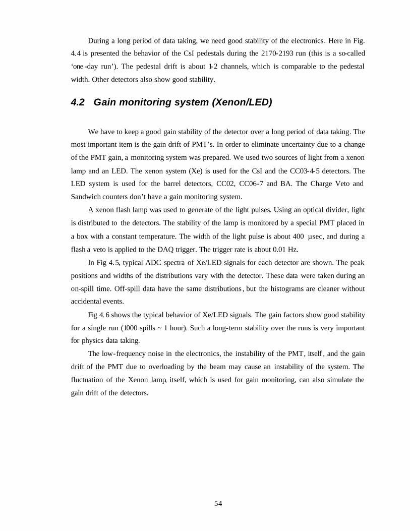
54

During a long period of data taking, we need good stability of the electronics. Here in Fig.

4.4 is presented the behavior of the CsI pedestals during the 2170-2193 run (this is a so-called

‘one -day run’). The pedestal drift is about 1-2 channels, which is comparable to the pedestal

width. Other detectors also show good stability.

4.2 Gain monitoring system (Xenon/LED)

We have to keep a good gain stability of the detector over a long period of data taking. The

most important item is the gain drift of PMT’s. In order to eliminate uncertainty due to a change

of the PMT gain, a monitoring system was prepared. We used two sources of light from a xenon

lamp and an LED. The xenon system (Xe) is used for the CsI and the CC03-4-5 detectors. The

LED system is used for the barrel detectors, CC02, CC06-7 and BA. The Charge Veto and

Sandwich counters don’t have a gain monitoring system.

A xenon flash lamp was used to generate of the light pulses. Using an optical divider, light

is distributed to the detectors. The stability of the lamp is monitored by a special PMT placed in

a box with a constant temperature. The width of the light pulse is about 400 µsec, and during a

flash a veto is applied to the DAQ trigger. The trigger rate is about 0.01 Hz.

In Fig 4.5, typical ADC spectra of Xe/LED signals for each detector are shown. The peak

positions and widths of the distributions vary with the detector. These data were taken during an

on-spill time. Off-spill data have the same distributions , but the histograms are cleaner without

accidental events.

Fig 4. 6 shows the typical behavior of Xe/LED signals. The gain factors show good stability

for a single run (1000 spills ~ 1 hour). Such a long-term stability over the runs is very important

for physics data taking.

The low-frequency noise in the electronics, the instability of the PMT, itself , and the gain

drift of the PMT due to overloading by the beam may cause an instability of the system. The

fluctuation of the Xenon lamp, itself, which is used for gain monitoring, can also simulate the

gain drift of the detectors.

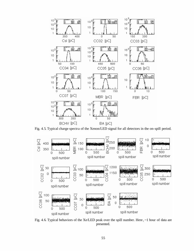
55

Fig. 4.5. Typical charge spectra of the Xenon/LED signal for all detectors in the on-spill period.

Fig. 4.6. Typical behaviors of the Xe/LED peak over the spill number. Here , ~1 hour of data are

presented.

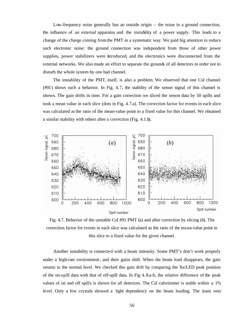
56

Low-frequency noise generally has an outside origin – the noise in a ground connection,

the influence of an external apparatus and the instability of a power supply. This leads to a

change of the charge coming from the PMT in a systematic way. We paid big attention to reduce

such electronic noise: the ground connection was independent from those of other power

supplies, power stabilizers were introduced, and the electronics were disconnected from the

external networks. We also made an effort to separate the grounds of all detectors in order not to

disturb the whole system by one bad channel.

The instability of the PMT, itself, is also a problem. We observed that one CsI channel

(#91) shows such a behavior. In Fig. 4.7, the stability of the xenon signal of this channel is

shown. The gain drifts in time. For a gain correction we sliced the xenon data by 50 spills and

took a mean value in each slice (dots in Fig. 4.7.a). The correction factor for events in each slice

was calculated as the ratio of the mean-value point to a fixed value for this channel. We obtained

a similar stability with others after a correction (Fig. 4.1.b).

Fig. 4.7. Behavior of the unstable CsI #91 PMT (a) and after correction by slicing (b). The

correction factor for events in each slice was calculated as the ratio of the mean-value point in

this slice to a fixed value for the given channel.

Another instability is connecte d with a beam intensity. Some PMT’s don’t work properly

under a high-rate environment , and their gains shift. When the beam load disappears, the gain

returns to the normal level. We checked this gain drift by comparing the Xe/LED peak position

of the on-spill data with that of off-spill data. In Fig 4. 8.a-b, the relative difference of the peak

values of on and off spills is shown for all detectors. The CsI calorimeter is stable within a 1%

level. Only a few crystals showed a light dependency on the beam loading. The main veto

)(a )(b

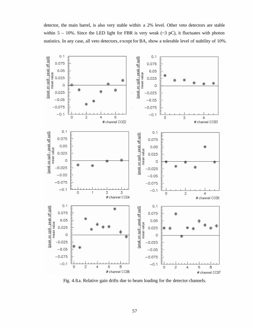
57

detector, the main barrel, is also very stable within a 2% level. Other veto detectors are stable

within 5 – 10%. Since the LED light for FBR is very weak (~3 pC), it fluctuates with photon

statistics. In any case, all veto detectors, except for BA, show a tolerable level of stability of 10%.

Fig. 4.8.a. Relative gain drifts due to beam loading for the detector channels.

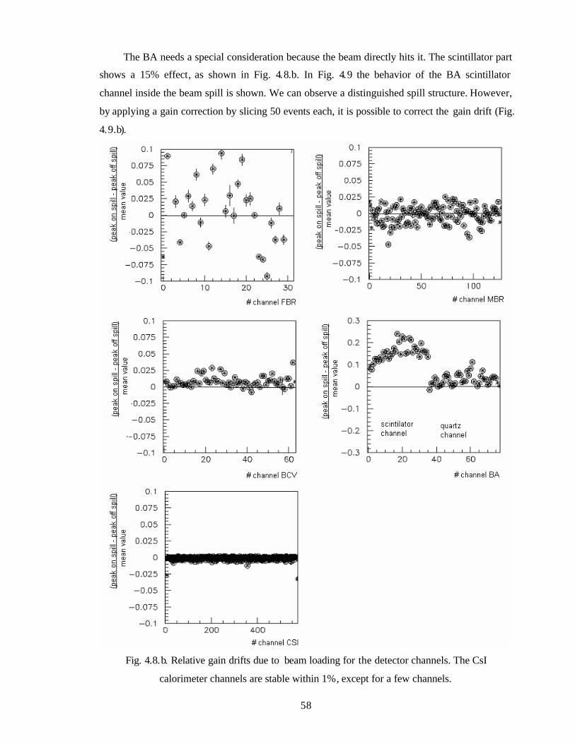
58

The BA needs a special consideration because the beam directly hits it. The scintillator part

shows a 15% effect, as shown in Fig. 4.8.b. In Fig. 4.9 the behavior of the BA scintillator

channel inside the beam spill is shown. We can observe a distinguished spill structure. However,

by applying a gain correction by slicing 50 events each, it is possible to correct the gain drift (Fig.

4.9.b).

Fig. 4.8.b. Relative gain drifts due to beam loading for the detector channels. The CsI

calorimeter channels are stable within 1%, except for a few channels.

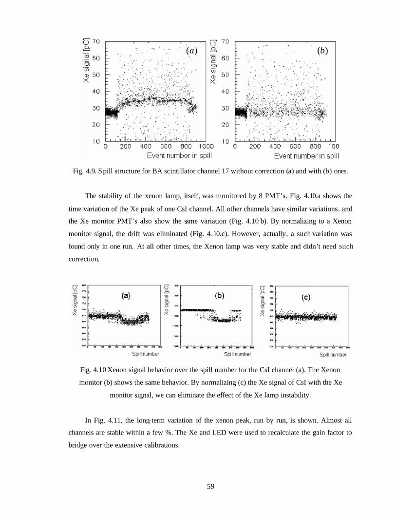
59

Fig. 4.9. Spill structure for BA scintillator channel 17 without correction (a) and with (b) ones.

The stability of the xenon lamp, itself, was monitored by 8 PMT’s. Fig. 4.10.a shows the

time variation of the Xe peak of one CsI channel. All other channels have similar variations. and

the Xe monitor PMT’s also show the same variation (Fig. 4.10.b). By normalizing to a Xenon

monitor signal, the drift was eliminated (Fig. 4.10.c). However, actually, a such variation was

found only in one run. At all other times, the Xenon lamp was very stable and didn’t need such

correction.

Fig. 4.10 Xenon signal behavior over the spill number for the CsI channel (a). The Xenon

monitor (b) shows the same behavior. By normalizing (c) the Xe signal of CsI with the Xe

monitor signal, we can eliminate the effect of the Xe lamp instability.

In Fig. 4.11, the long-term variation of the xenon peak, run by run, is shown. Almost all

channels are stable within a few %. The Xe and LED were used to recalculate the gain factor to

bridge over the extensive calibrations.

)(a )(b

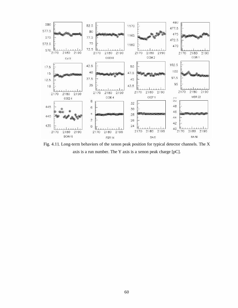
60

Fig. 4.11. Long-term behaviors of the xenon peak position for typical detector channels. The X

axis is a run number. The Y axis is a xenon peak charge [pC].

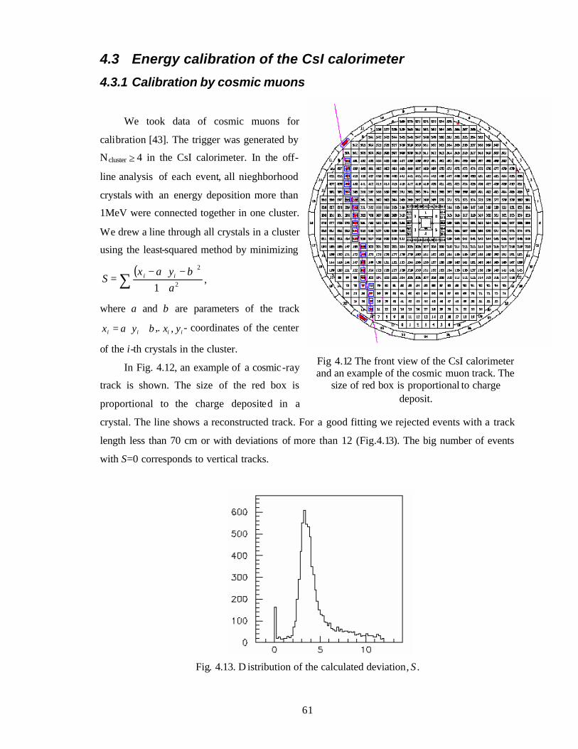
61

4.3 Energy calibration of the CsI calorimeter

4.3.1 Calibration by cosmic muons

We took data of cosmic muons for

calibration [43]. The trigger was generated by

Ncluster ≥ 4 in the CsI calorimeter. In the off-

line analysis of each event, all nieghborhood

crystals with an energy deposition more than

1MeV were connected together in one cluster.

We drew a line through all crystals in a cluster

using the least-squared method by minimizing

( )∑ +−⋅−

=2

2

1 abyax

S ii ,

where a and b are parameters of the track

byax ii +⋅= ,. ii yx , - coordinates of the center

of the i-th crystals in the cluster.

In Fig. 4.12, an example of a cosmic-ray

track is shown. The size of the red box is

proportional to the charge deposited in a

crystal. The line shows a reconstructed track. For a good fitting we rejected events with a track

length less than 70 cm or with deviations of more than 12 (Fig.4.13). The big number of events

with S=0 corresponds to vertical tracks.

Fig. 4.13. D istribution of the calculated deviation, S .

Fig 4.12 The front view of the CsI calorimeter and an example of the cosmic muon track. The

size of red box is proportional to charge deposit.

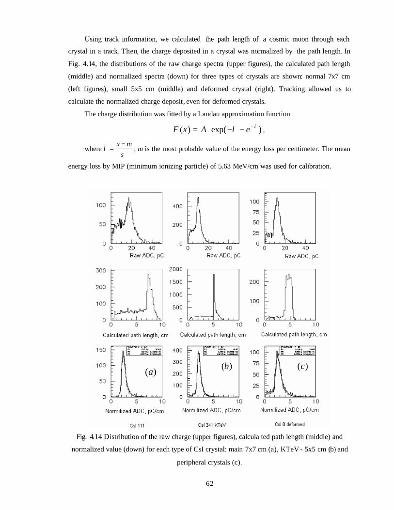
62

Using track information, we calculated the path length of a cosmic muon through each

crystal in a track. Then, the charge deposited in a crystal was normalized by the path length. In

Fig. 4.14, the distributions of the raw charge spectra (upper figures), the calculated path length

(middle) and normalized spectra (down) for three types of crystals are shown: normal 7x7 cm

(left figures), small 5x5 cm (middle) and deformed crystal (right). Tracking allowed us to

calculate the normalized charge deposit, even for deformed crystals.

The charge distribution was fitted by a Landau approximation function

)exp()( λλ −−−⋅= eAxF ,

whereσ

λmx −

= ; m is the most probable value of the energy loss per centimeter. The mean

energy loss by MIP (minimum ionizing particle) of 5.63 MeV/cm was used for calibration.

Fig. 4.14 Distribution of the raw charge (upper figures), calcula ted path length (middle) and

normalized value (down) for each type of CsI crystal: main 7x7 cm (a), KTeV - 5x5 cm (b) and

peripheral crystals (c).

)(c)(a

)(b

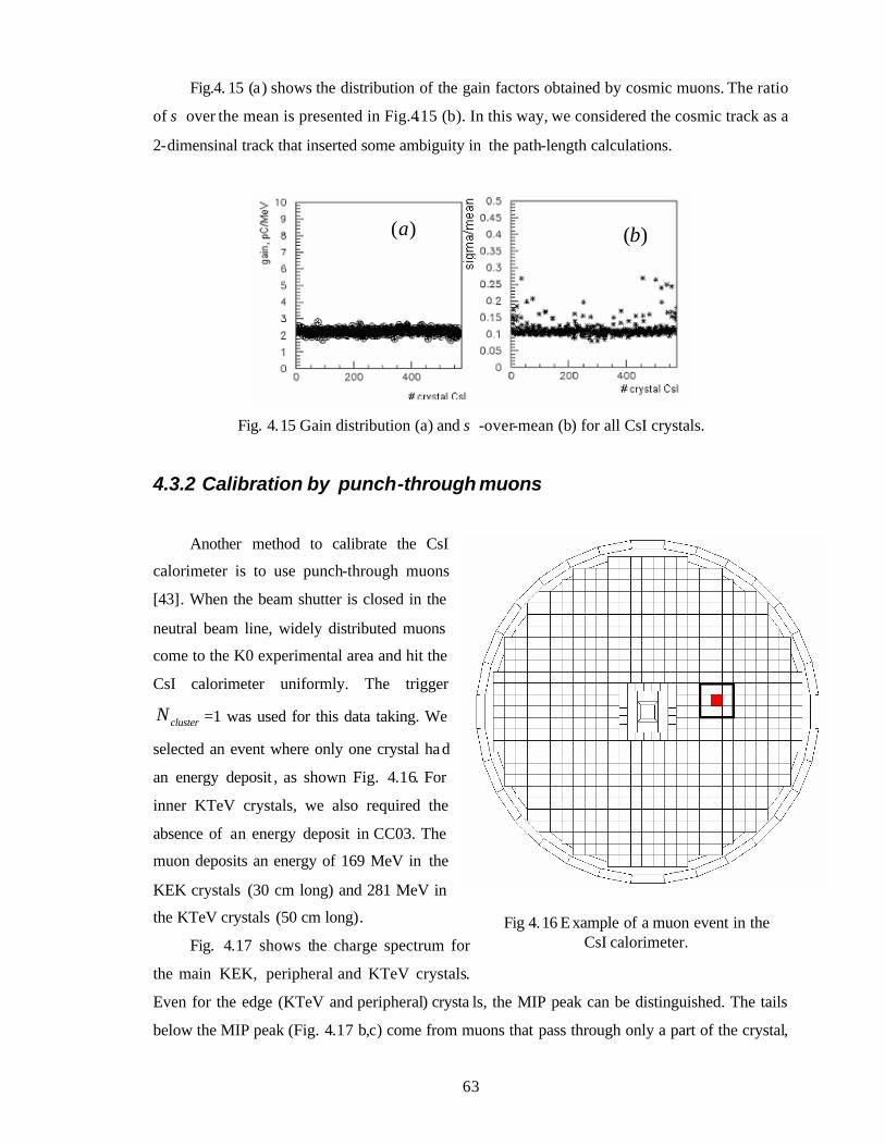
63

Fig 4.16 Example of a muon event in the CsI calorimeter.

Fig.4. 15 (a) shows the distribution of the gain factors obtained by cosmic muons. The ratio

of σ over the mean is presented in Fig.4.15 (b). In this way, we considered the cosmic track as a

2-dimensinal track that inserted some ambiguity in the path-length calculations.

Fig. 4.15 Gain distribution (a) and σ -over-mean (b) for all CsI crystals.

4.3.2 Calibration by punch-through muons

Another method to calibrate the CsI

calorimeter is to use punch-through muons

[43]. When the beam shutter is closed in the

neutral beam line, widely distributed muons

come to the K0 experimental area and hit the

CsI calorimeter uniformly. The trigger

clusterN =1 was used for this data taking. We

selected an event where only one crystal had

an energy deposit , as shown Fig. 4.16. For

inner KTeV crystals, we also required the

absence of an energy deposit in CC03. The

muon deposits an energy of 169 MeV in the

KEK crystals (30 cm long) and 281 MeV in

the KTeV crystals (50 cm long).

Fig. 4.17 shows the charge spectrum for

the main KEK, peripheral and KTeV crystals.

Even for the edge (KTeV and peripheral) crysta ls, the MIP peak can be distinguished. The tails

below the MIP peak (Fig. 4.17 b,c) come from muons that pass through only a part of the crystal,

)(a )(b

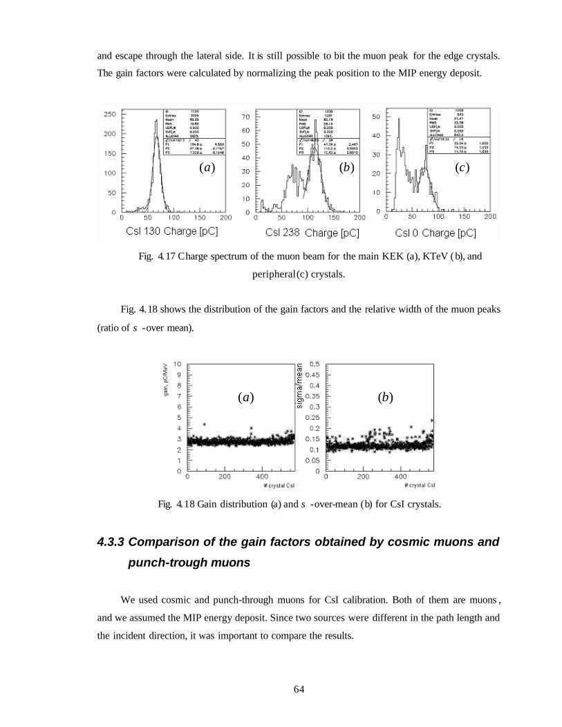
64

and escape through the lateral side. It is still possible to bit the muon peak for the edge crystals.

The gain factors were calculated by normalizing the peak position to the MIP energy deposit.

Fig. 4.17 Charge spectrum of the muon beam for the main KEK (a), KTeV (b), and

peripheral (c) crystals.

Fig. 4.18 shows the distribution of the gain factors and the relative width of the muon peaks

(ratio of σ -over mean).

Fig. 4.18 Gain distribution (a) and σ -over-mean (b) for CsI crystals.

4.3.3 Comparison of the gain factors obtained by cosmic muons and

punch-trough muons

We used cosmic and punch-through muons for CsI calibration. Both of them are muons ,

and we assumed the MIP energy deposit. Since two sources were different in the path length and

the incident direction, it was important to compare the results.

)(b)(a )(c

)(b)(a

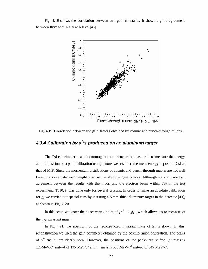
65

Fig. 4.19 shows the correlation between two gain constants. It shows a good agreement

between them within a few% level [43] .

Fig. 4.19. Correlation between the gain factors obtained by cosmic and punch-through muons.

4.3.4 Calibration by π 0’s produced on an aluminum target

The CsI calorimeter is an electromagnetic calorimeter that has a role to measure the energy

and hit position of a γ. In calibration using muons we assumed the mean energy deposit in CsI as

that of MIP. Since the momentum distributions of cosmic and punch-through muons are not well

known, a systematic error might exist in the absolute gain factors. Although we confirmed an

agreement between the results with the muon and the electron beam within 5% in the test

experiment , T510, it was done only for several crystals. In order to make an absolute calibration

for γ, we carried out special runs by inserting a 5 mm-thick aluminum target in the detector [43],

as shown in Fig. 4. 20.

In this setup we know the exact vertex point of γγπ →0 , which allows us to reconstruct

the γ γ invariant mass.

In Fig 4.21, the spectrum of the reconstructed invariant mass of 2γ is shown. In this

reconstruction we used the gain parameter obtained by the cosmic-muon calibration. The peaks

of π 0 and η are clearly seen. However, the positions of the peaks are shifted: π0 mass is

126MeV/c2 instead of 135 MeV/c 2 and η mass is 508 MeV/c 2 instead of 547 MeV/c2.

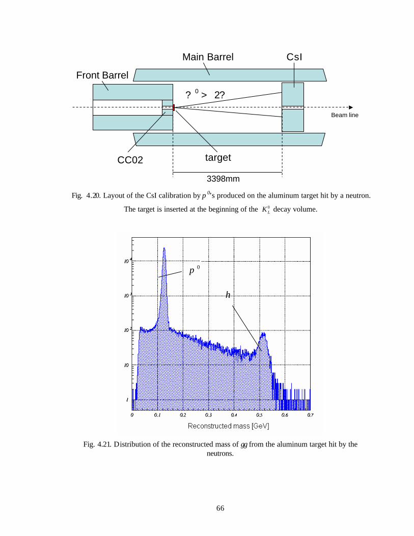
66

Fig. 4.20. Layout of the CsI calibration by π 0’s produced on the aluminum target hit by a neutron.

The target is inserted at the beginning of the 0LK decay volume.

Fig. 4.21. Distribution of the reconstructed mass of γγ from the aluminum target hit by the neutrons.

Main Barrel

Front Barrel

CC02

CsI

target

Beam line

? 0 > 2?

3398mm

0π

η

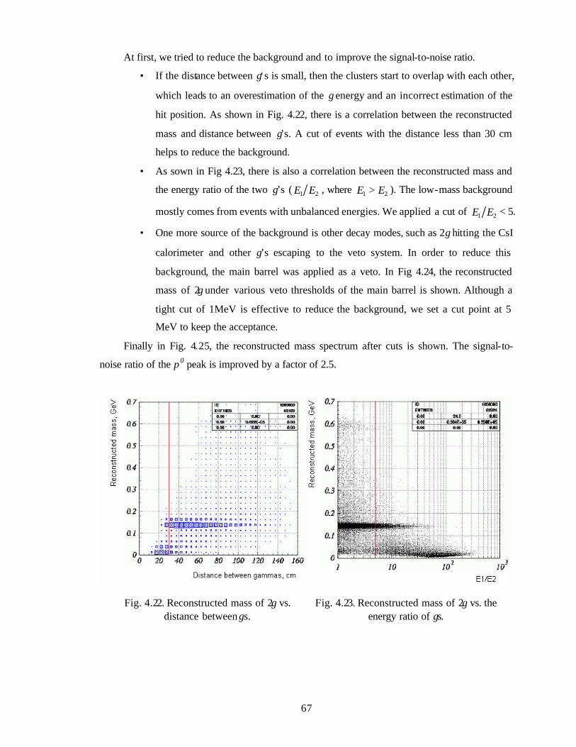
67

Fig. 4.22. Reconstructed mass of 2γ vs. distance between γs.

Fig. 4.23. Reconstructed mass of 2γ vs. the energy ratio of γs.

At first, we tried to reduce the background and to improve the signal-to-noise ratio.

• If the distance between γ‘s is small, then the clusters start to overlap with each other,

which leads to an overestimation of the γ energy and an incorrect estimation of the

hit position. As shown in Fig. 4.22, there is a correlation between the reconstructed

mass and distance between γ’s. A cut of events with the distance less than 30 cm

helps to reduce the background.

• As sown in Fig 4.23, there is also a correlation between the reconstructed mass and

the energy ratio of the two γ’s ( 21 EE , where 21 EE > ). The low-mass background

mostly comes from events with unbalanced energies. We applied a cut of 21 EE < 5.

• One more source of the background is other decay modes, such as 2γ hitting the CsI

calorimeter and other γ’s escaping to the veto system. In order to reduce this

background, the main barrel was applied as a veto. In Fig 4.24, the reconstructed

mass of 2γ under various veto thresholds of the main barrel is shown. Although a

tight cut of 1MeV is effective to reduce the background, we set a cut point at 5

MeV to keep the acceptance.

Finally in Fig. 4.25, the reconstructed mass spectrum after cuts is shown. The signal-to-

noise ratio of the π0 peak is improved by a factor of 2.5.

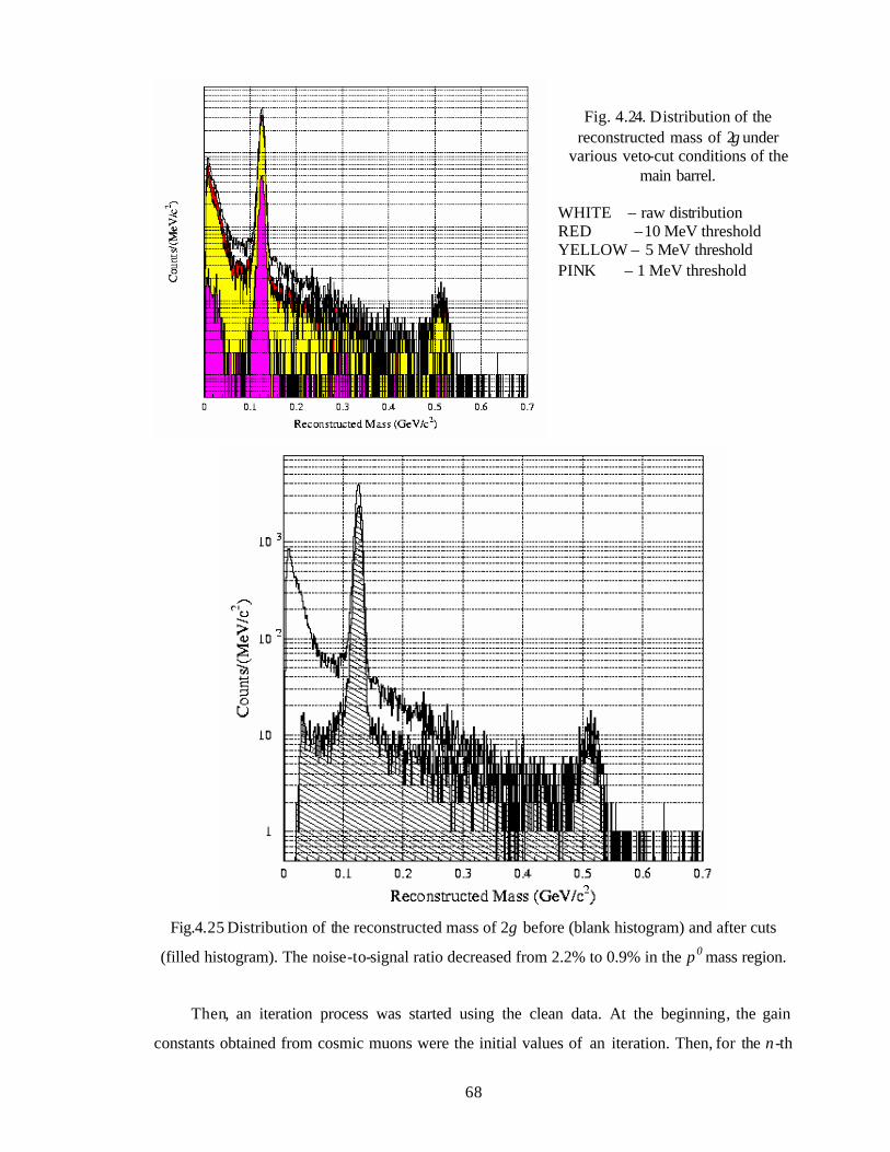
68

Fig.4.25 Distribution of the reconstructed mass of 2γ before (blank histogram) and after cuts

(filled histogram). The noise-to-signal ratio decreased from 2.2% to 0.9% in the π0 mass region.

Then, an iteration process was started using the clean data. At the beginning, the gain

constants obtained from cosmic muons were the initial values of an iteration. Then, for the n -th

Fig. 4.24. Distribution of the reconstructed mass of 2γ under

various veto-cut conditions of the main barrel.

WHITE – raw distribution RED –10 MeV threshold YELLOW – 5 MeV threshold PINK – 1 MeV threshold

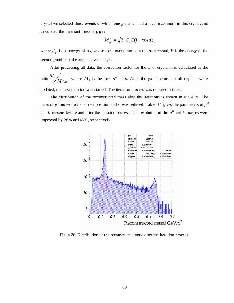
69

crystal we selected those events of which one γ cluster had a local maximum in this crystal, and

calculated the invariant mass of γ γ as

)cos1(2 θγγ −⋅= EEM nn ,

where nE is the energy of a γ whose local maximum is in the n -th crystal, E is the energy of the

second γ and θ is the angle between 2 γs.

After processing all data, the correction factor for the n -th crystal was calculated as the

ratioγγ

πnM

M, where πM is the true π0 mass. After the gain factors for all crystals were

updated, the next iteration was started. The iteration process was repeated 5 times.

The distribution of the reconstructed mass after the iterations is shown in Fig 4. 26. The

mass of π 0 moved to its correct position and σ was reduced. Table 4.1 gives the parameters of π 0

and η mesons before and after the iteration process. The resolution of the π0 and η masses were

improved by 28% and 45% , respectively.

Fig. 4.26. Distribution of the reconstructed mass after the iteration process.

Reconstructed mass,[GeV/c2]

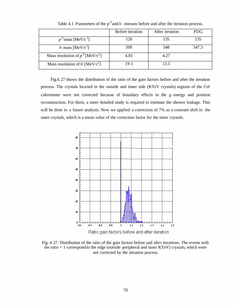
70

Table 4.1. Parameters of the π 0 and η -mesons before and after the iteration process.

Before iteration After iteration PDG

π 0 mass [MeV/c 2] 126 135 135

η mass [MeV/c2] 508 548 547.3

Mass resolution of π 0 [MeV/c2] 4.81 4.27

Mass resolution of η [MeV/c2] 19.1 13.5

Fig.4. 27 shows the distribution of the ratio of the gain factors before and after the iteration

process. The crystals loca ted in the outside and inner side (KTeV crystals) regions of the CsI

calorimeter were not corrected because of boundary effects in the γ energy and position

reconstruction. For them, a more detailed study is required to estimate the shower leakage. This

will be done in a future analysis. Now we applied a correction of 7% as a constant shift to the

outer crystals, which is a mean value of the correction factor for the inner crystals.

Fig. 4.27. Distribution of the ratio of the gain factors before and afte r iterations. The events with

the ratio = 1 correspond to the edge (outside peripheral and inner KTeV) crystals, which were not corrected by the iteration process.

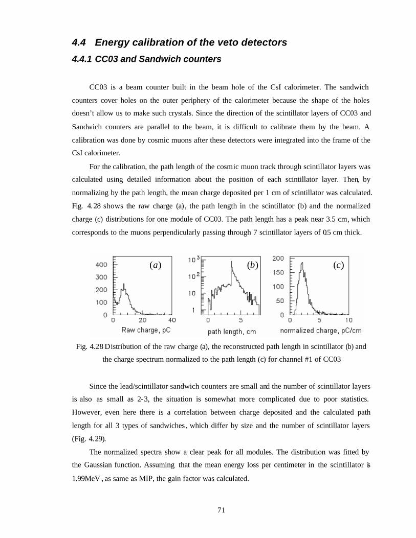
71

4.4 Energy calibration of the veto detectors

4.4.1 CC03 and Sandwich counters

CC03 is a beam counter built in the beam hole of the CsI calorimeter. The sandwich

counters cover holes on the outer periphery of the calorimeter because the shape of the holes

doesn’t allow us to make such crystals. Since the direction of the scintillator layers of CC03 and

Sandwich counters are parallel to the beam, it is difficult to calibrate them by the beam. A

calibration was done by cosmic muons after these detectors were integrated into the frame of the

CsI calorimeter.

For the calibration, the path length of the cosmic muon track through scintillator layers was

calculated using detailed information about the position of each scintillator layer. Then, by

normalizing by the path length, the mean charge deposited per 1 cm of scintillator was calculated.

Fig. 4.28 shows the raw charge (a) , the path length in the scintillator (b) and the normalized

charge (c) distributions for one module of CC03. The path length has a peak near 3.5 cm, which

corresponds to the muons perpendicularly passing through 7 scintillator layers of 0.5 cm thick.

Fig. 4.28 Distribution of the raw charge (a), the reconstructed path length in scintillator (b) and

the charge spectrum normalized to the path length (c) for channel #1 of CC03

Since the lead/scintillator sandwich counters are small and the number of scintillator layers

is also as small as 2-3, the situation is somewhat more complicated due to poor statistics.

However, even here there is a correlation between charge deposited and the calculated path

length for all 3 types of sandwiches , which differ by size and the number of scintillator layers

(Fig. 4.29).

The normalized spectra show a clear peak for all modules. The distribution was fitted by

the Gaussian function. Assuming that the mean energy loss per centimeter in the scintillator is

1.99MeV , as same as MIP, the gain factor was calculated.

)(a )(b )(c

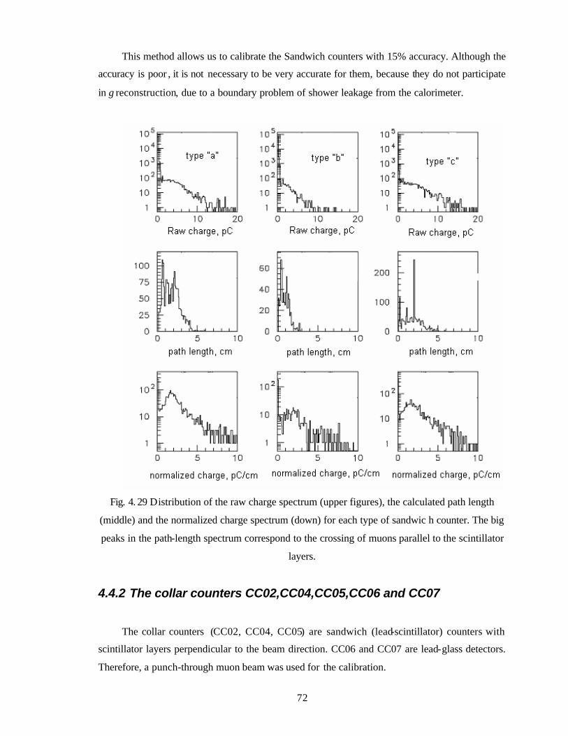
72

This method allows us to calibrate the Sandwich counters with 15% accuracy. Although the

accuracy is poor , it is not necessary to be very accurate for them, because they do not participate

in γ reconstruction, due to a boundary problem of shower leakage from the calorimeter.

Fig. 4. 29 Distribution of the raw charge spectrum (upper figures), the calculated path length

(middle) and the normalized charge spectrum (down) for each type of sandwic h counter. The big

peaks in the path-length spectrum correspond to the crossing of muons parallel to the scintillator

layers.

4.4.2 The collar counters CC02,CC04,CC05,CC06 and CC07

The collar counters (CC02, CC04, CC05) are sandwich (lead-scintillator) counters with

scintillator layers perpendicular to the beam direction. CC06 and CC07 are lead-glass detectors.

Therefore, a punch-through muon beam was used for the calibration.

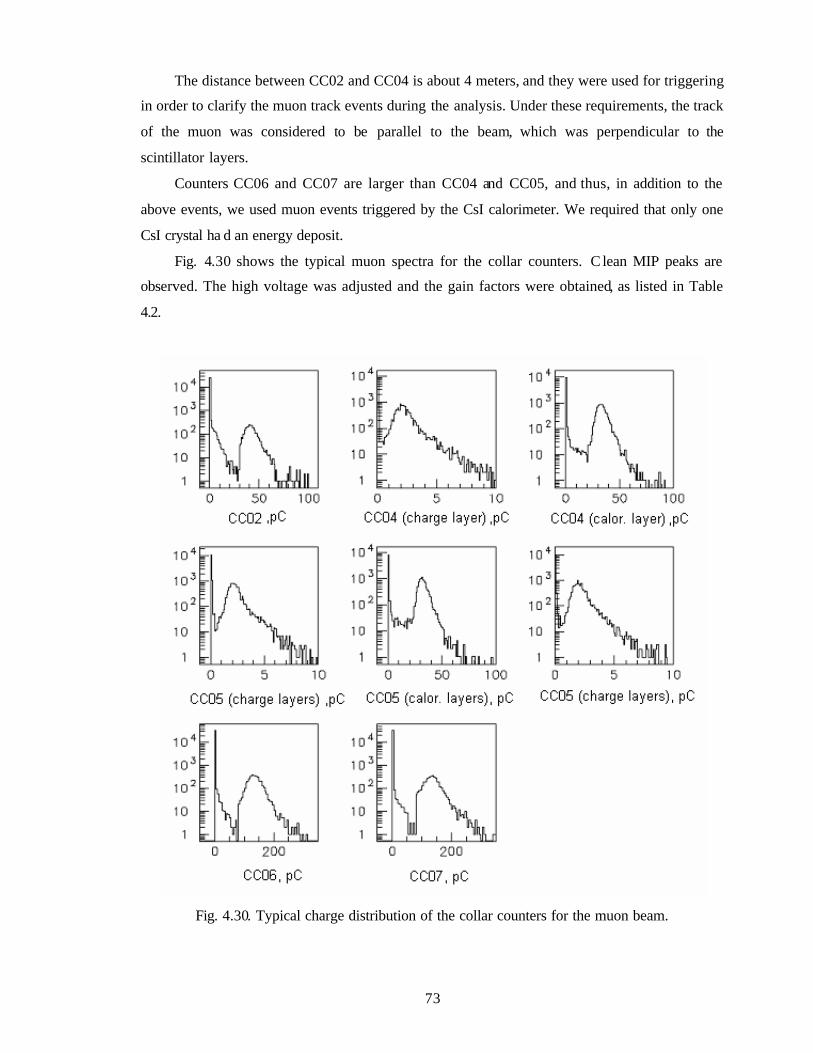
73

The distance between CC02 and CC04 is about 4 meters, and they were used for triggering

in order to clarify the muon track events during the analysis. Under these requirements, the track

of the muon was considered to be parallel to the beam, which was perpendicular to the

scintillator layers.

Counters CC06 and CC07 are larger than CC04 and CC05, and thus, in addition to the

above events, we used muon events triggered by the CsI calorimeter. We required that only one

CsI crystal ha d an energy deposit.

Fig. 4.30 shows the typical muon spectra for the collar counters. C lean MIP peaks are

observed. The high voltage was adjusted and the gain factors were obtained, as listed in Table

4.2.

Fig. 4.30. Typical charge distribution of the collar counters for the muon beam.

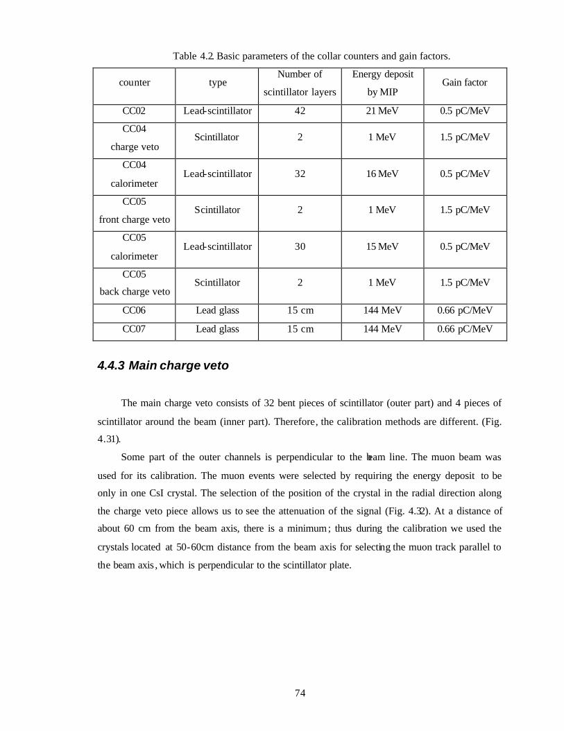
74

Table 4.2. Basic parameters of the collar counters and gain factors.

counter type Number of

scintillator layers

Energy deposit

by MIP Gain factor

CC02 Lead-scintillator 42 21 MeV 0.5 pC/MeV

CC04

charge veto Scintillator 2 1 MeV 1.5 pC/MeV

CC04

calorimeter Lead-scintillator 32 16 MeV 0.5 pC/MeV

CC05

front charge veto Scintillator 2 1 MeV 1.5 pC/MeV

CC05

calorimeter Lead-scintillator 30 15 MeV 0.5 pC/MeV

CC05

back charge veto Scintillator 2 1 MeV 1.5 pC/MeV

CC06 Lead glass 15 cm 144 MeV 0.66 pC/MeV

CC07 Lead glass 15 cm 144 MeV 0.66 pC/MeV

4.4.3 Main charge veto

The main charge veto consists of 32 bent pieces of scintillator (outer part) and 4 pieces of

scintillator around the beam (inner part). Therefore, the calibration methods are different. (Fig.

4.31).

Some part of the outer channels is perpendicular to the beam line. The muon beam was

used for its calibration. The muon events were selected by requiring the energy deposit to be

only in one CsI crystal. The selection of the position of the crystal in the radial direction along

the charge veto piece allows us to see the attenuation of the signal (Fig. 4.32). At a distance of

about 60 cm from the beam axis, there is a minimum; thus during the calibration we used the

crystals located at 50-60cm distance from the beam axis for selecting the muon track parallel to

the beam axis , which is perpendicular to the scintillator plate.

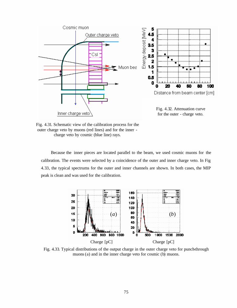
75

Fig. 4.31. Schematic view of the calibration process for the outer charge veto by muons (red lines) and for the inner -

charge veto by cosmic (blue line) rays.

Fig. 4.32. Attenuation curve for the outer - charge veto.

Because the inner pieces are located parallel to the beam, we used cosmic muons for the

calibration. The events were selected by a coincidence of the outer and inner charge veto. In Fig

4.33, the typical spectrums for the outer and inner channels are shown. In both cases, the MIP

peak is clean and was used for the calibration.

Fig. 4.33. Typical distributions of the output charge in the outer charge veto for punch-through

muons (a) and in the inner charge veto for cosmic (b) muons.

Charge [pC] Charge [pC]

)(a )(b

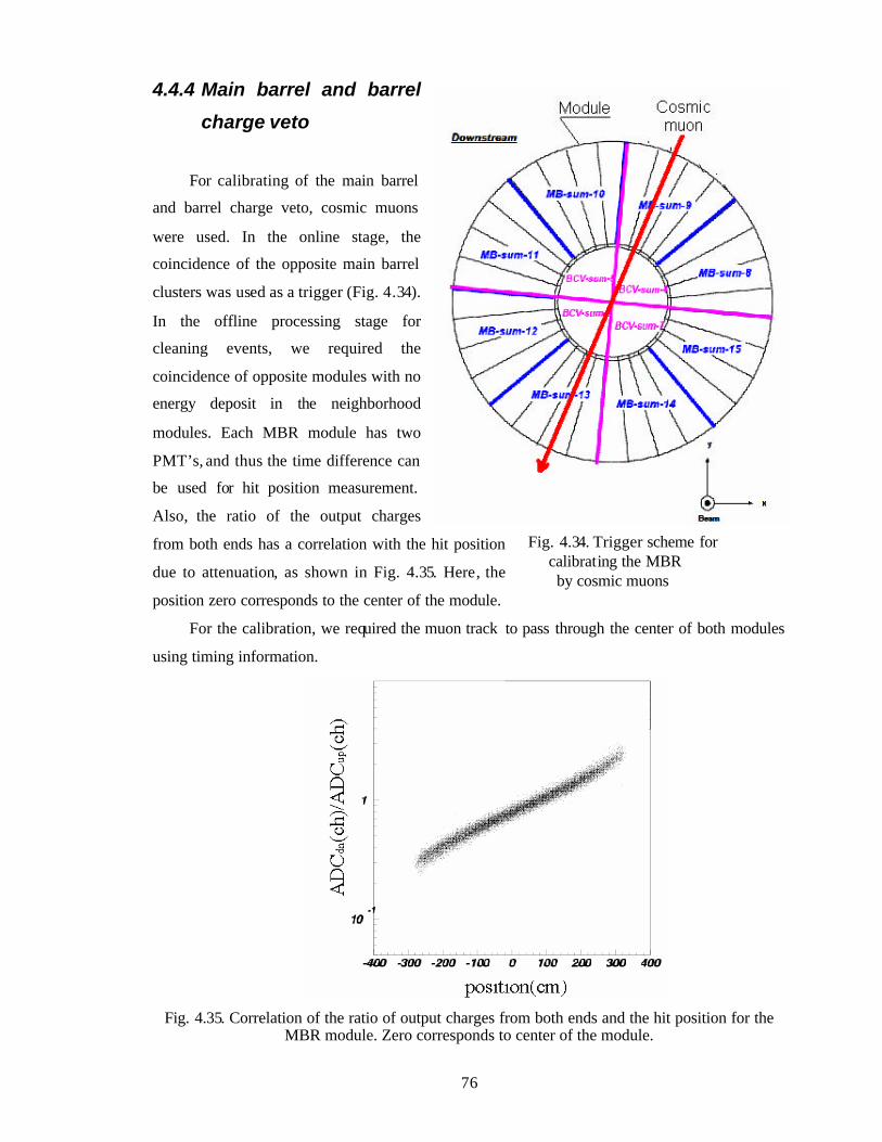
76

4.4.4 Main barrel and barrel

charge veto

For calibrating of the main barrel

and barrel charge veto, cosmic muons

were used. In the online stage, the

coincidence of the opposite main barrel

clusters was used as a trigger (Fig. 4.34).

In the offline processing stage for

cleaning events, we required the

coincidence of opposite modules with no

energy deposit in the neighborhood

modules. Each MBR module has two

PMT’s, and thus the time difference can

be used for hit position measurement.

Also, the ratio of the output charges

from both ends has a correlation with the hit position

due to attenuation, as shown in Fig. 4.35. Here, the

position zero corresponds to the center of the module.

For the calibration, we required the muon track to pass through the center of both modules

using timing information.

Fig. 4.35. Correlation of the ratio of output charges from both ends and the hit position for the MBR module. Zero corresponds to center of the module.

Fig. 4.34. Trigger scheme for calibrating the MBR by cosmic muons

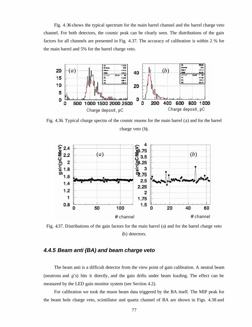
77

Fig. 4.36 shows the typical spectrum for the main barrel channel and the barrel charge veto

channel. For both detectors, the cosmic peak can be clearly seen. The distributions of the gain

factors for all channels are presented in Fig. 4.37. The accuracy of calibration is within 2 % for

the main barrel and 5% for the barrel charge veto.

Fig. 4.36. Typical charge spectra of the cosmic muons for the main barrel (a) and for the barrel

charge veto (b).

Fig. 4.37. Distributions of the gain factors for the main barrel (a) and for the barrel charge veto

(b) detectors.

4.4.5 Beam anti (BA) and beam charge veto

The beam anti is a difficult detector from the view point of gain calibration. A neutral beam

(neutrons and γ’s) hits it directly, and the gain drifts under beam loading. The effect can be

measured by the LED gain monitor system (see Section 4.2).

For calibration we took the muon beam data triggered by the BA itself. The MIP peak for

the beam hole charge veto, scintillator and quartz channel of BA are shown in Figs. 4.38 and

)(a )(b

)(a )(b

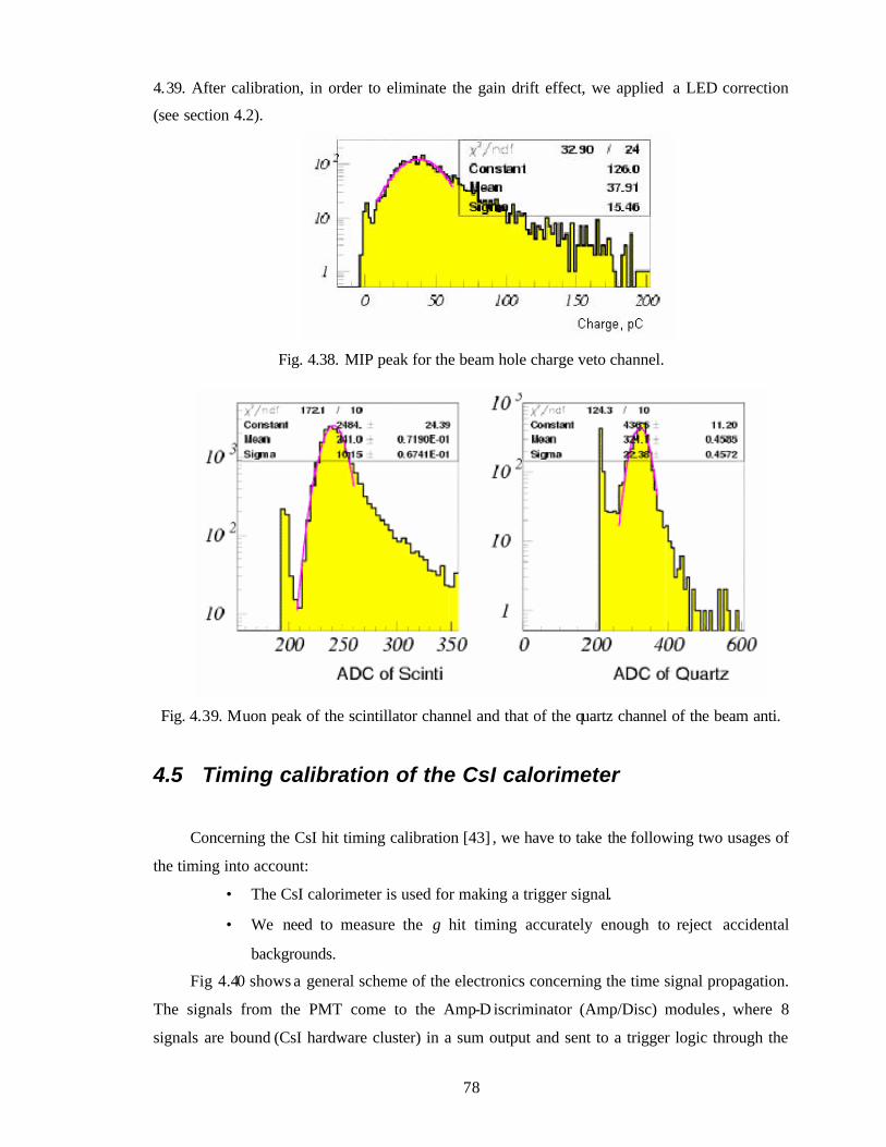
78

4.39. After calibration, in order to eliminate the gain drift effect, we applied a LED correction

(see section 4.2).

Fig. 4.38. MIP peak for the beam hole charge veto channel.

Fig. 4.39. Muon peak of the scintillator channel and that of the quartz channel of the beam anti.

4.5 Timing calibration of the CsI calorimeter

Concerning the CsI hit timing calibration [43] , we have to take the following two usages of

the timing into account:

• The CsI calorimeter is used for making a trigger signal.

• We need to measure the γ hit timing accurately enough to reject accidental

backgrounds.

Fig 4.40 shows a general scheme of the electronics concerning the time signal propagation.

The signals from the PMT come to the Amp-D iscriminator (Amp/Disc) modules , where 8

signals are bound (CsI hardware cluster) in a sum output and sent to a trigger logic through the

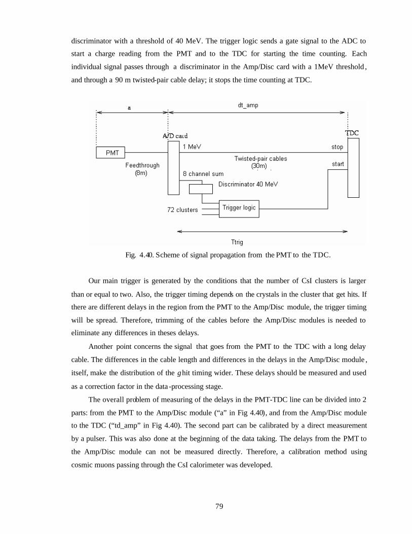
79

discriminator with a threshold of 40 MeV. The trigger logic sends a gate signal to the ADC to

start a charge reading from the PMT and to the TDC for starting the time counting. Each

individual signal passes through a discriminator in the Amp/Disc card with a 1MeV threshold ,

and through a 90 m twisted-pair cable delay; it stops the time counting at TDC.

Fig. 4.40. Scheme of signal propagation from the PMT to the TDC.

Our main trigger is generated by the conditions that the number of CsI clusters is larger

than or equal to two. Also, the trigger timing depends on the crystals in the cluster that get hits. If

there are different delays in the region from the PMT to the Amp/Disc module, the trigger timing

will be spread. Therefore, trimming of the cables before the Amp/Disc modules is needed to

eliminate any differences in theses delays.

Another point concerns the signal that goes from the PMT to the TDC with a long delay

cable. The differences in the cable length and differences in the delays in the Amp/Disc module ,

itself, make the distribution of the γ hit timing wider. These delays should be measured and used

as a correction factor in the data -processing stage.

The overall problem of measuring of the delays in the PMT-TDC line can be divided into 2

parts: from the PMT to the Amp/Disc module (“a” in Fig 4.40), and from the Amp/Disc module

to the TDC (“td_amp” in Fig 4.40). The second part can be calibrated by a direct measurement

by a pulser. This was also done at the beginning of the data taking. The delays from the PMT to

the Amp/Disc module can not be measured directly. Therefore, a calibration method using

cosmic muons passing through the CsI calorimeter was developed.

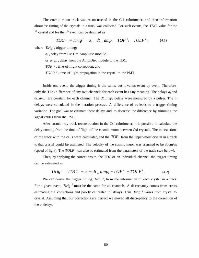
80

The cosmic muon track was reconstructed in the CsI calorimeter , and then information

about the timing of the crystals in a track was collected. For such events, the TDCi value for the

ith crystal and for the jth event can be descried as

ij

ij

iij

ij TOLPTOFampdtaTtrigTDC ++++= _ , (4.1)

where Ttrig j , trigger timing;

ai , delay from PMT to Amp/Disc module ;

dt_ampi , delay from the Amp/Disc module to the TDC;

TOF i j , time-of-flight correction; and

TOLPi j , time-of-light-propagation in the crystal to the PMT.

Inside one event, the trigger timing is the same, but it varies event by event. Therefore ,

only the TDC difference of any two channels for each event has a ny meaning. The delays ai and

dt_amp i are constant for each channel. The dt_amp i delays were measured by a pulser. The a i

delays were calculated in the iteration process. A difference of a i leads to a trigger timing

variation. The goal was to estimate these delays and to decrease the difference by trimming the

signal cables from the PMT.

After cosmic –ray track reconstruction in the CsI calorimeter, it is possible to calculate the

delay coming from the time of flight of the cosmic muon between CsI crystals. The intersections

of the track with the cells were calculated, and the iTOF from the upper-most crystal in a track

to that crystal could be estimated. The velocity of the cosmic muon was assumed to be 30cm/ns

(speed of light). The TOLP i can also be estimated from the parameters of the track (see below).

Then, by applying the corrections to the TDC of an individual channel, the trigger timing

can be estimated as

jii

jiii

jj TOLPTOFampdtaTDCTtrig −−−−= _ . (4.2)

We can derive the trigger timing, Ttrig j, from the information of each crystal in a track.

For a given event, Ttrig j must be the same for all channels. A discrepancy comes from errors

estimating the corrections and poorly calibrated a i delays. Thus Ttrig j varies from crystal to

crystal. Assuming that our corrections are perfect we moved all discrepancy to the correction of

the ai delays.

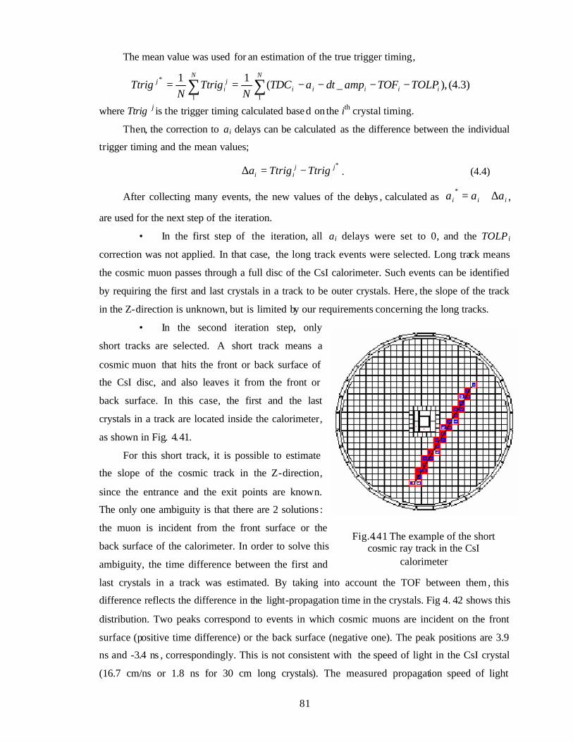
81

Fig.4.41 The example of the short cosmic ray track in the CsI

calorimeter

The mean value was used for an estimation of the true trigger timing,

)3.4(,)_(11

11

* ∑∑ −−−−==N

iiiii

Nj

ij TOLPTOFampdtaTDC

NTtrig

NTtrig

where Ttrig j is the trigger timing calculated based on the ith crystal timing.

Then, the correction to ai delays can be calculated as the difference between the individual

trigger timing and the mean values;

*jj

ii TtrigTtriga −=∆ . (4.4)

After collecting many events, the new values of the delays , calculated as iii aaa ∆+=*,

are used for the next step of the iteration.

• In the first step of the iteration, all ai delays were set to 0, and the TOLP i

correction was not applied. In that case, the long track events were selected. Long track means

the cosmic muon passes through a full disc of the CsI calorimeter. Such events can be identified

by requiring the first and last crystals in a track to be outer crystals. Here, the slope of the track

in the Z-direction is unknown, but is limited by our requirements concerning the long tracks.

• In the second iteration step, only

short tracks are selected. A short track means a

cosmic muon that hits the front or back surface of

the CsI disc, and also leaves it from the front or

back surface. In this case, the first and the last

crystals in a track are located inside the calorimeter,

as shown in Fig. 4.41.

For this short track, it is possible to estimate

the slope of the cosmic track in the Z-direction,

since the entrance and the exit points are known.

The only one ambiguity is that there are 2 solutions :

the muon is incident from the front surface or the

back surface of the calorimeter. In order to solve this

ambiguity, the time difference between the first and

last crystals in a track was estimated. By taking into account the TOF between them, this

difference reflects the difference in the light-propagation time in the crystals. Fig 4. 42 shows this

distribution. Two peaks correspond to events in which cosmic muons are incident on the front

surface (positive time difference) or the back surface (negative one). The peak positions are 3.9

ns and -3.4 ns , correspondingly. This is not consistent with the speed of light in the CsI crystal

(16.7 cm/ns or 1.8 ns for 30 cm long crystals). The measured propagation speed of light

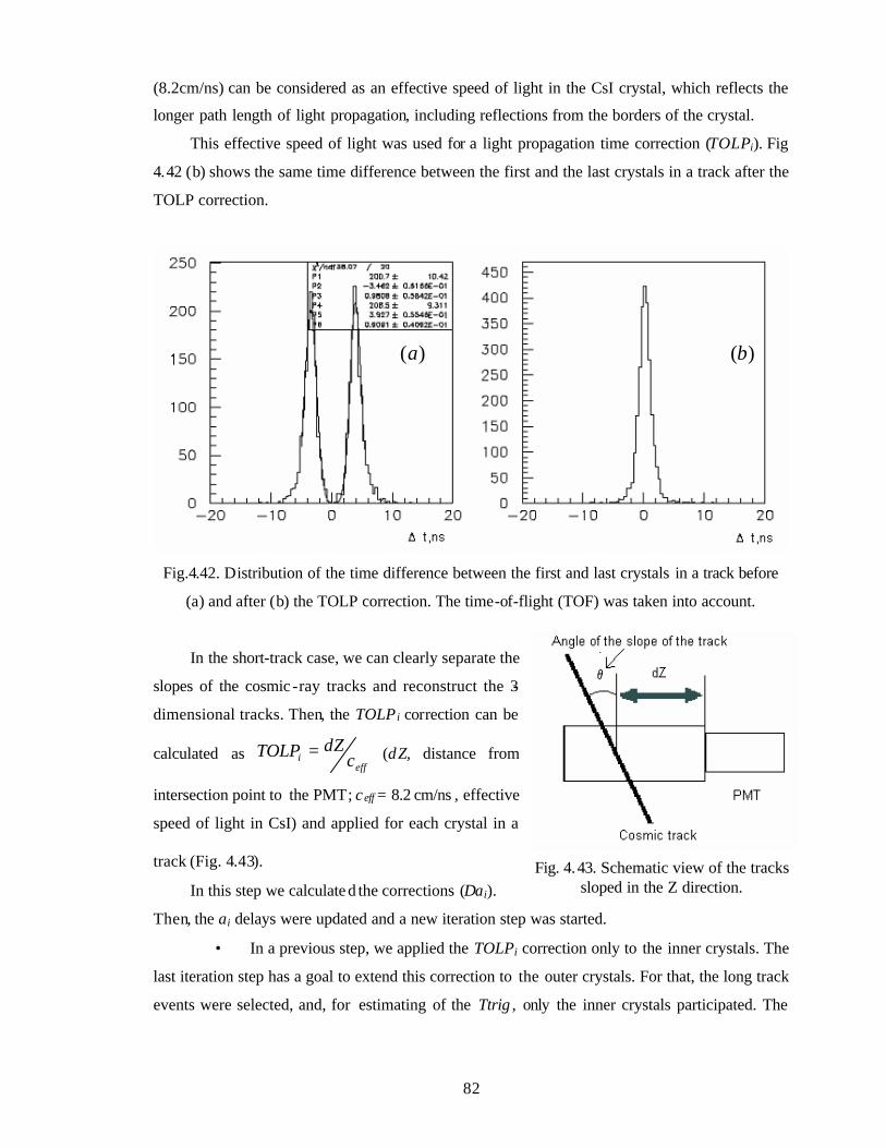
82

(8.2cm/ns) can be considered as an effective speed of light in the CsI crystal, which reflects the

longer path length of light propagation, including reflections from the borders of the crystal.

This effective speed of light was used for a light propagation time correction (TOLPi). Fig

4.42 (b) shows the same time difference between the first and the last crystals in a track after the

TOLP correction.

Fig.4.42. Distribution of the time difference between the first and last crystals in a track before

(a) and after (b) the TOLP correction. The time-of-flight (TOF) was taken into account.

In the short-track case, we can clearly separate the

slopes of the cosmic -ray tracks and reconstruct the 3-

dimensional tracks. Then, the TOLP i correction can be

calculated as eff

i cdZTOLP = (dZ, distance from

intersection point to the PMT; ceff = 8.2 cm/ns , effective

speed of light in CsI) and applied for each crystal in a

track (Fig. 4.43).

In this step we calculate d the corrections (∆ai).

Then, the ai delays were updated and a new iteration step was started.

• In a previous step, we applied the TOLPi correction only to the inner crystals. The

last iteration step has a goal to extend this correction to the outer crystals. For that, the long track

events were selected, and, for estimating of the Ttrig , only the inner crystals participated. The

Fig. 4.43. Schematic view of the tracks sloped in the Z direction.

)(a )(b

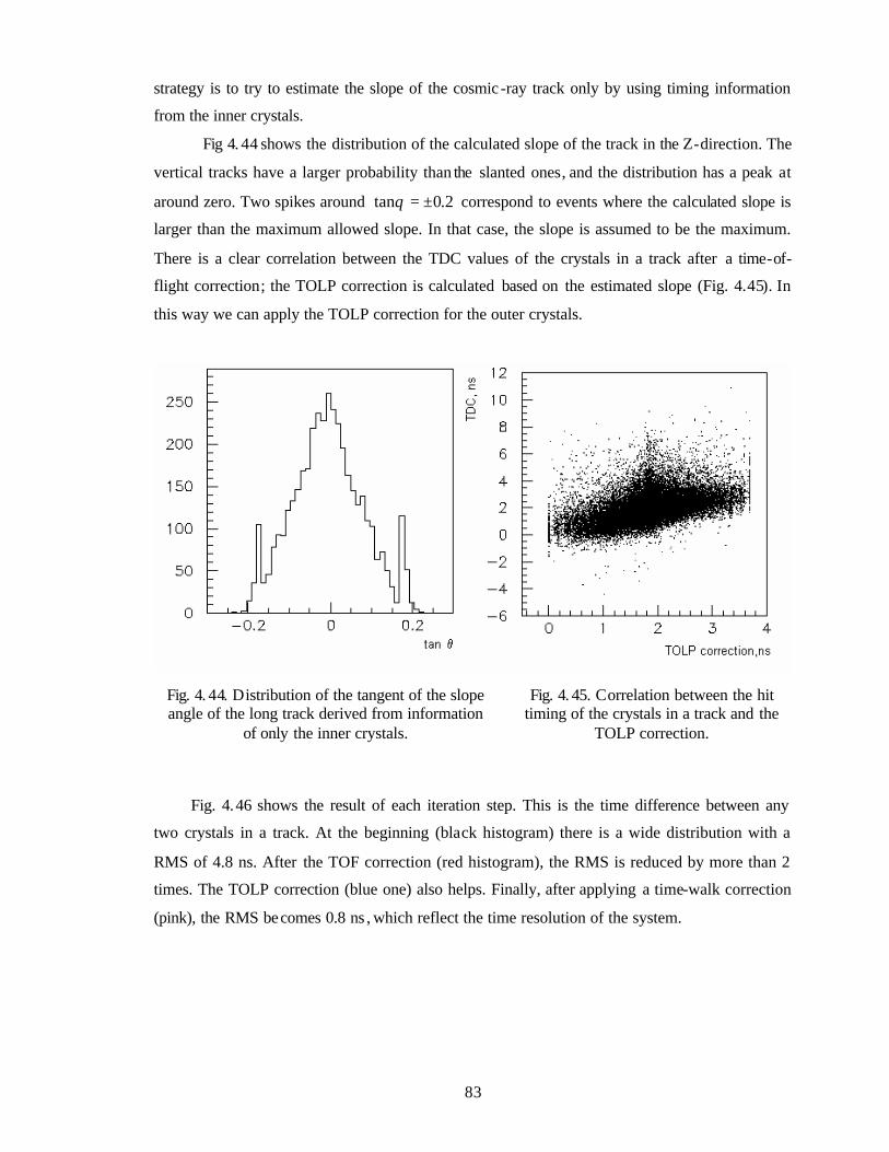
83

strategy is to try to estimate the slope of the cosmic -ray track only by using timing information

from the inner crystals.

Fig 4. 44 shows the distribution of the calculated slope of the track in the Z-direction. The

vertical tracks have a larger probability than the slanted ones, and the distribution has a peak at

around zero. Two spikes around 2.0tan ±=θ correspond to events where the calculated slope is

larger than the maximum allowed slope. In that case, the slope is assumed to be the maximum.

There is a clear correlation between the TDC values of the crystals in a track after a time-of-

flight correction; the TOLP correction is calculated based on the estimated slope (Fig. 4.45). In

this way we can apply the TOLP correction for the outer crystals.

Fig. 4.46 shows the result of each iteration step. This is the time difference between any

two crystals in a track. At the beginning (black histogram) there is a wide distribution with a

RMS of 4.8 ns. After the TOF correction (red histogram), the RMS is reduced by more than 2

times. The TOLP correction (blue one) also helps. Finally, after applying a time-walk correction

(pink), the RMS becomes 0.8 ns , which reflect the time resolution of the system.

Fig. 4. 44. Distribution of the tangent of the slope angle of the long track derived from information

of only the inner crystals.

Fig. 4. 45. Correlation between the hit timing of the crystals in a track and the

TOLP correction.

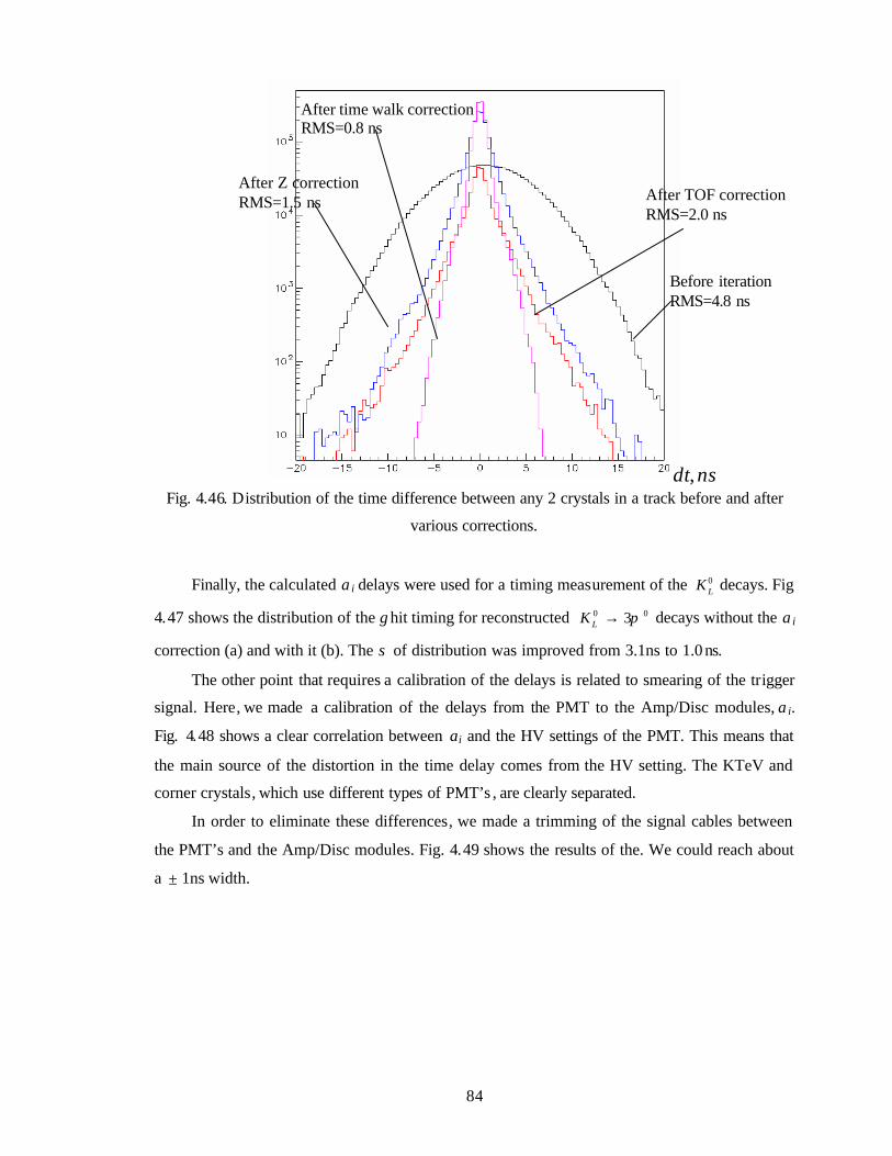
84

Fig. 4.46. Distribution of the time difference between any 2 crystals in a track before and after

various corrections.

Finally, the calculated a i delays were used for a timing measurement of the 0LK decays. Fig

4.47 shows the distribution of the γ hit timing for reconstructed 00 3π→LK decays without the a i

correction (a) and with it (b). The σ of distribution was improved from 3.1ns to 1.0 ns.

The other point that requires a calibration of the delays is related to smearing of the trigger

signal. Here, we made a calibration of the delays from the PMT to the Amp/Disc modules, a i.

Fig. 4.48 shows a clear correlation between ai and the HV settings of the PMT. This means that

the main source of the distortion in the time delay comes from the HV setting. The KTeV and

corner crystals, which use different types of PMT’s , are clearly separated.

In order to eliminate these differences, we made a trimming of the signal cables between

the PMT’s and the Amp/Disc modules. Fig. 4.49 shows the results of the. We could reach about

a ± 1ns width.

After Z correction RMS=1.5 ns After TOF correction

RMS=2.0 ns

nsdt,

After time walk correction RMS=0.8 ns

Before iteration RMS=4.8 ns

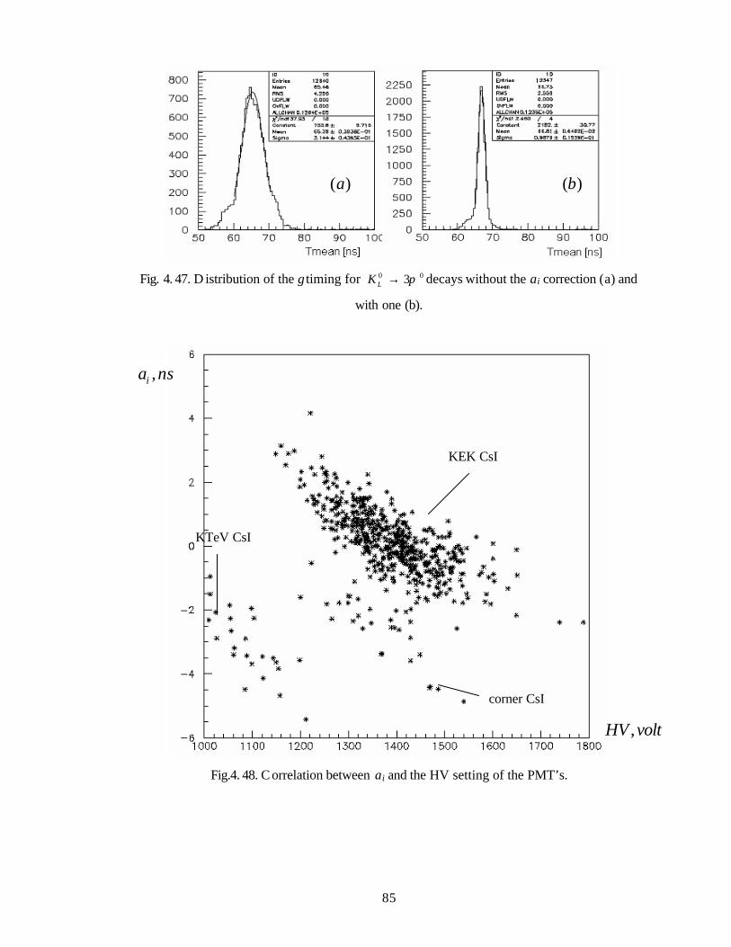
85

Fig. 4. 47. D istribution of the γ timing for 00 3π→LK decays without the ai correction (a) and

with one (b).

Fig.4. 48. C orrelation between ai and the HV setting of the PMT’s.

KEK CsI

KTeV CsI

corner CsI

nsai ,

voltHV ,

)(a )(b

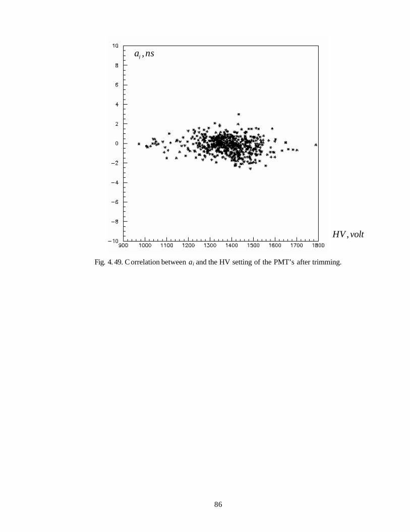
86

Fig. 4. 49. C orrelation between ai and the HV setting of the PMT’s after trimming.

nsai ,

voltHV ,

87

Chapter 5

Analysis

5.1 Data skimming

During the run we collected about 6 Tb of physics data. Because this is very large, it was

very hard to process these data directly. Also, the data files contained data for all triggers. In

order to remove non-physics events, we did a skim of the data. Also, additional cuts for

preliminary identification of events were applied to separate the data into streams characterized

by the number of γ clusters. Then, the 2γ, 4γ, 6γ streams were used to reconstruct the vvKL00 π→

and γγ→0LK , 00 2π→LK , 00 3π→LK decays, correspondingly. This data skimming saved

processing time and reduced the data size of each stream.

During the run we simultaneously collected data with various triggers:

• Pedestal trigger (1Hz)

• Cosmic trigger (~60Hz, during off-spill)

• Xe/LED trigger (~1Hz)

• Ncluster ≥2 – phys ics trigger (~200Hz)

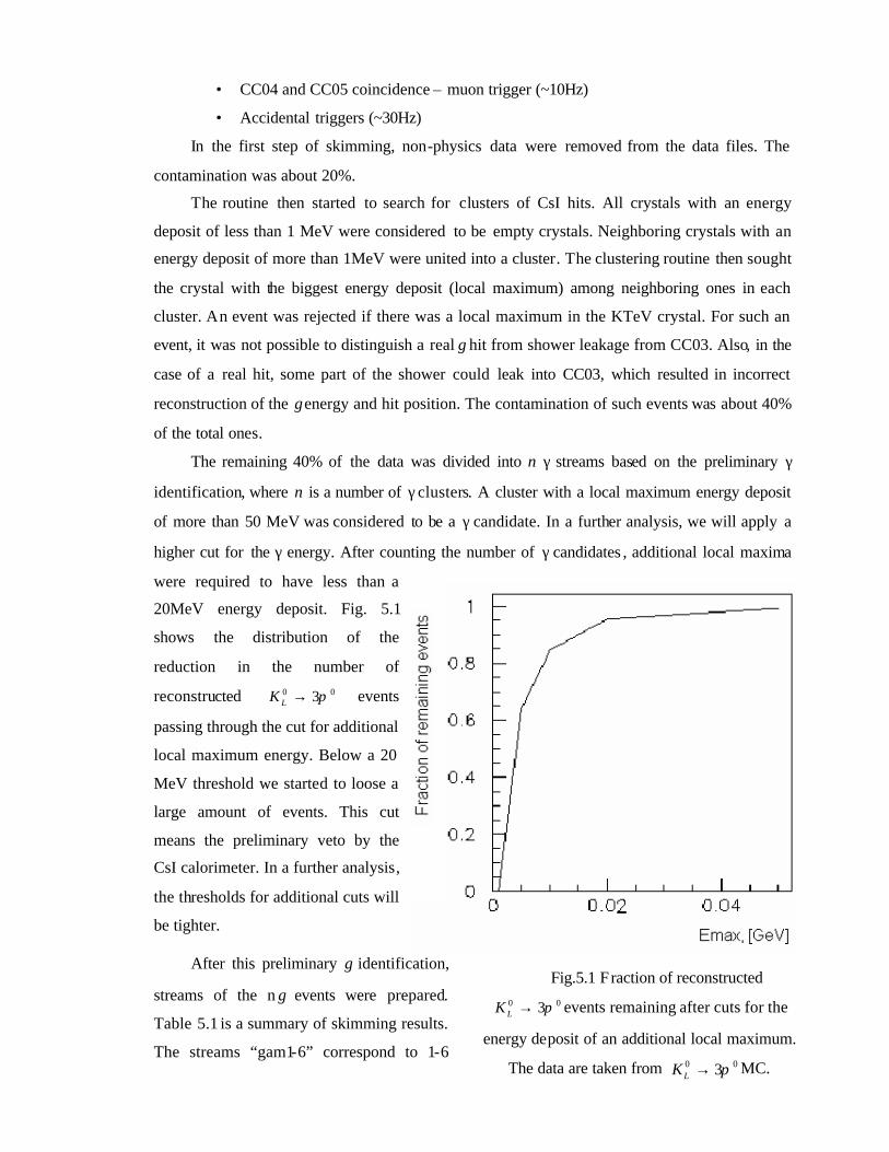
88

• CC04 and CC05 coincidence – muon trigger (~10Hz)

• Accidental triggers (~30Hz)

In the first step of skimming, non-physics data were removed from the data files. The

contamination was about 20%.

The routine then started to search for clusters of CsI hits. All crystals with an energy

deposit of less than 1 MeV were considered to be empty crystals. Neighboring crystals with an

energy deposit of more than 1MeV were united into a cluster. The clustering routine then sought

the crystal with the biggest energy deposit (local maximum) among neighboring ones in each

cluster. An event was rejected if there was a local maximum in the KTeV crystal. For such an

event, it was not possible to distinguish a real γ hit from shower leakage from CC03. Also, in the

case of a real hit, some part of the shower could leak into CC03, which resulted in incorrect

reconstruction of the γ energy and hit position. The contamination of such events was about 40%

of the total ones.

The remaining 40% of the data was divided into n γ streams based on the preliminary γ

identification, where n is a number of γ clusters. A cluster with a local maximum energy deposit

of more than 50 MeV was considered to be a γ candidate. In a further analysis, we will apply a

higher cut for the γ energy. After counting the number of γ candidates , additional local maxima

were required to have less than a

20MeV energy deposit. Fig. 5.1

shows the distribution of the

reduction in the number of

reconstructed 00 3π→LK events

passing through the cut for additional

local maximum energy. Below a 20

MeV threshold we started to loose a

large amount of events. This cut

means the preliminary veto by the

CsI calorimeter. In a further analysis,

the thresholds for additional cuts will

be tighter.

After this preliminary γ identification,

streams of the n γ events were prepared.

Table 5.1 is a summary of skimming results.

The streams “gam1-6” correspond to 1-6

Fig.5.1 Fraction of reconstructed 00 3π→LK events remaining after cuts for the

energy deposit of an additional local maximum.

The data are taken from 00 3π→LK MC.

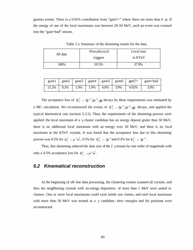
89

gamma events. There is a 0.02% contribution from “gam7+” where there are more than 6 γs. If

the energy of one of the local maximums was between 20-50 MeV, such an event was counted

into the “gam+bad” stream.

Table 5.1. Summary of the skimming results for the data.

gam1 gam2 gam3 gam4 gam5 gam6 gam7+ gam+bad

15.2% 9.3% 1.9% 1.9% 4.0% 3.9% 0.02% 5.0%

The acceptance loss of γγππ ,2,3 000 →LK decays by these requirements was estimated by

a MC calculation. We reconstructed the events of γγππ ,2,3 000 →LK decays , and applied the

typical kinematical cuts (section 5.3.5). Then, the requirements of the skimming process were

applied: the local maximum of a γ cluster candidate has an energy deposit grater than 50 MeV,

there is no additional local maximum with an energy over 20 MeV, and there is no local

maximum in the KTeV crystals. It was found that the acceptance loss due to this skimming

process was 0.5% for vvKL00 π→ , 0.5% for 00 2π→LK and 0.2% for 00 3π→LK .

Thus, this skimming reduced the data size of the 2 γ stream by one order of magnitude with

only a 0.5% acceptance loss for vvKL00 π→ .

5.2 Kinematical reconstruction

At the beginning of off-line data processing, the clustering routine scanned all crystals, and

then the neighboring crystals with an energy deposition of more than 1 MeV were united in

clusters. One or more local maximums could exist inside one cluster, and each local maximum

with more than 50 MeV was treated as a γ candidate ; their energies and hit positions were

reconstructed.

All data Non-physical

triggers

Local max

in KTeV

100% 19.5% 37.9%

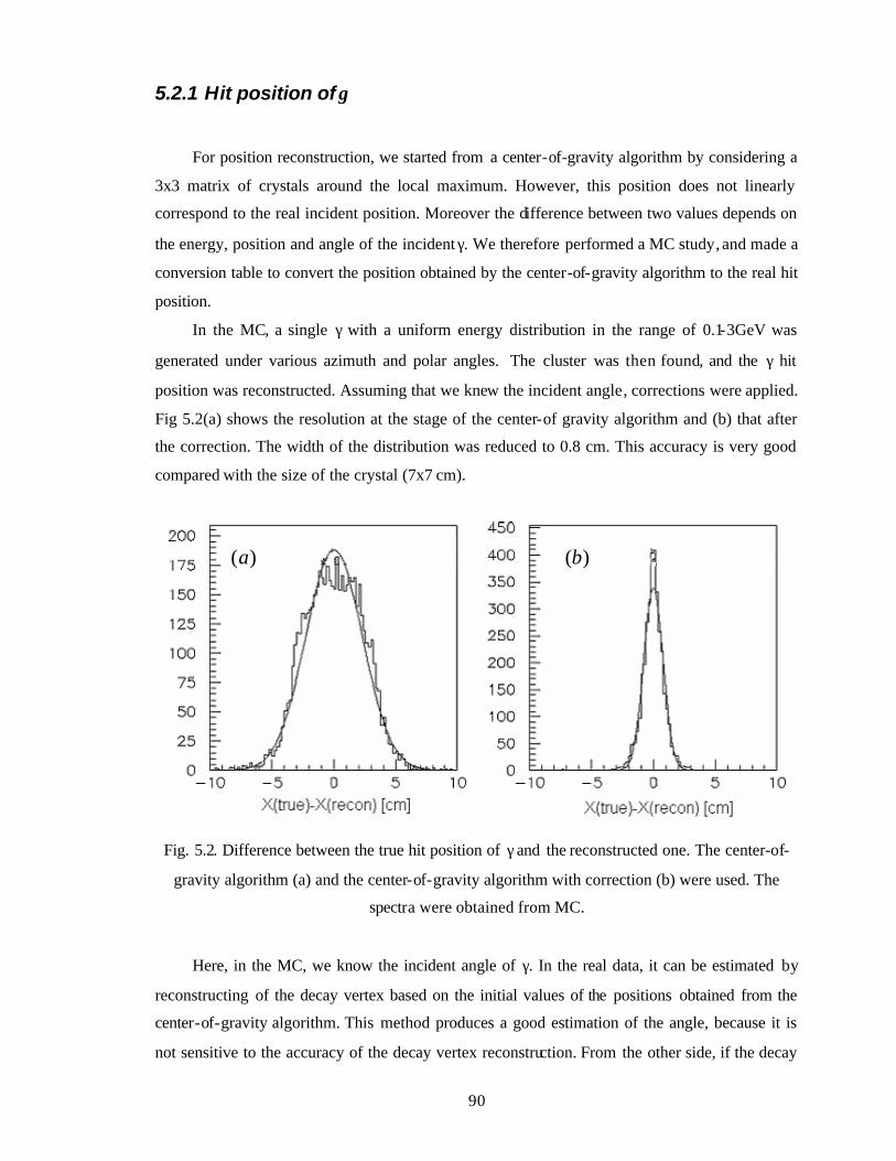
90

5.2.1 Hit position of γ

For position reconstruction, we started from a center-of-gravity algorithm by considering a

3x3 matrix of crystals around the local maximum. However, this position does not linearly

correspond to the real incident position. Moreover the difference between two values depends on

the energy, position and angle of the incident γ. We therefore performed a MC study, and made a

conversion table to convert the position obtained by the center-of-gravity algorithm to the real hit

position.

In the MC, a single γ with a uniform energy distribution in the range of 0.1-3GeV was

generated under various azimuth and polar angles. The cluster was then found, and the γ hit

position was reconstructed. Assuming that we knew the incident angle, corrections were applied.

Fig 5.2(a) shows the resolution at the stage of the center-of gravity algorithm and (b) that after

the correction. The width of the distribution was reduced to 0.8 cm. This accuracy is very good

compared with the size of the crystal (7x7 cm).

Fig. 5.2. Difference between the true hit position of γ and the reconstructed one. The center-of-

gravity algorithm (a) and the center-of-gravity algorithm with correction (b) were used. The

spectra were obtained from MC.

Here, in the MC, we know the incident angle of γ. In the real data, it can be estimated by

reconstructing of the decay vertex based on the initial values of the positions obtained from the

center-of-gravity algorithm. This method produces a good estimation of the angle, because it is

not sensitive to the accuracy of the decay vertex reconstruction. From the other side, if the decay

)(a )(b

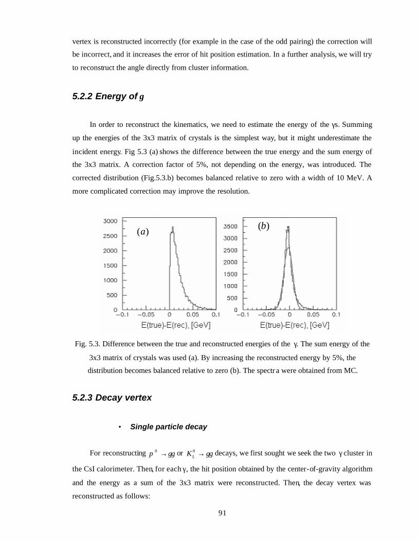
91

vertex is reconstructed incorrectly (for example in the case of the odd pairing) the correction will

be incorrect, and it increases the error of hit position estimation. In a further analysis, we will try

to reconstruct the angle directly from cluster information.

5.2.2 Energy of γ

In order to reconstruct the kinematics, we need to estimate the energy of the γs. Summing

up the energies of the 3x3 matrix of crystals is the simplest way, but it might underestimate the

incident energy. Fig 5.3 (a) shows the difference between the true energy and the sum energy of

the 3x3 matrix. A correction factor of 5%, not depending on the energy, was introduced. The

corrected distribution (Fig.5.3.b) becomes balanced relative to zero with a width of 10 MeV. A

more complicated correction may improve the resolution.

Fig. 5.3. Difference between the true and reconstructed energies of the γ. The sum energy of the

3x3 matrix of crystals was used (a). By increasing the reconstructed energy by 5%, the

distribution becomes balanced relative to zero (b). The spectr a were obtained from MC.

5.2.3 Decay vertex

• Single particle decay

For reconstructing γγπ →0 or γγ→0LK decays, we first sought we seek the two γ cluster in

the CsI calorimeter. Then, for each γ, the hit position obtained by the center-of-gravity algorithm

and the energy as a sum of the 3x3 matrix were reconstructed. Then, the decay vertex was

reconstructed as follows:

)(a )(b

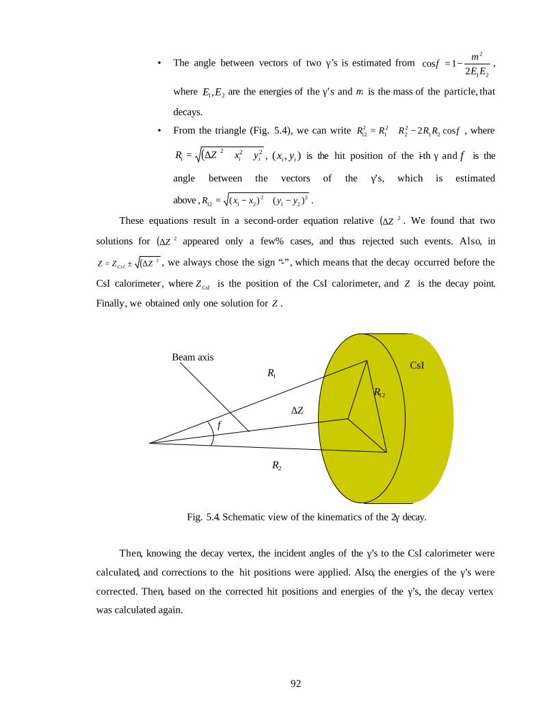
92

• The angle between vectors of two γ’s is estimated from 21

2

21cos

EEm

−=φ ,

where 21,EE are the energies of the γ’s and m is the mass of the particle, that

decays.

• From the triangle (Fig. 5.4), we can write φcos2 2122

21

212 RRRRR −+= , where

( ) 222iii yxZR ++∆= , ),( ii yx is the hit position of the i-th γ and φ is the

angle between the vectors of the γ’s, which is estimated

above , 221

22112 )()( yyxxR −+−= .

These equations result in a second-order equation relative ( )2Z∆ . We found that two

solutions for ( )2Z∆ appeared only a few% cases, and thus rejected such events. Also, in

( )2ZZZ CsI ∆±= , we always chose the sign “-”, which means that the decay occurred before the

CsI calorimeter , where CsIZ is the position of the CsI calorimeter, and Z is the decay point.

Finally, we obtained only one solution for Z .

Fig. 5.4. Schematic view of the kinematics of the 2γ decay.

Then, knowing the decay vertex, the incident angles of the γ’s to the CsI calorimeter were

calculated, and corrections to the hit positions were applied. Also, the energies of the γ’s were

corrected. Then, based on the corrected hit positions and energies of the γ’s, the decay vertex

was calculated again.

12R

2R

1R

Z∆φ

CsI Beam axis

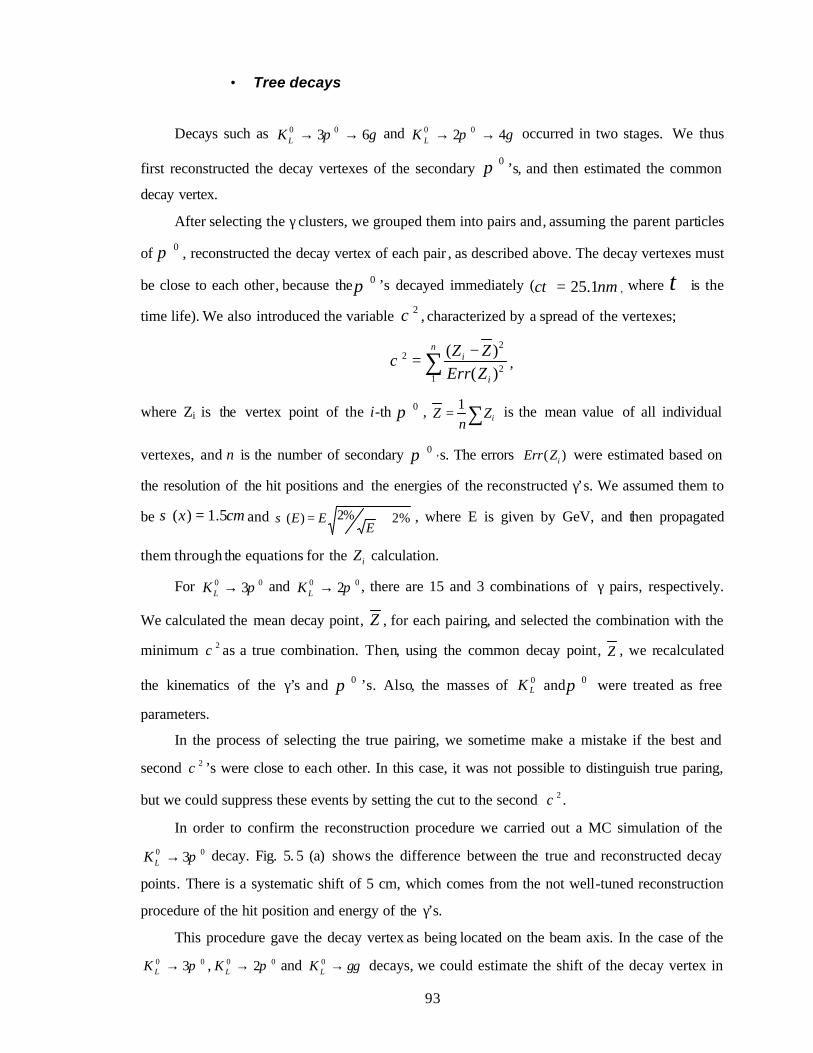
93

• Tree decays

Decays such as γπ 63 00 →→LK and γπ 42 00 →→LK occurred in two stages. We thus

first reconstructed the decay vertexes of the secondary 0π ’s, and then estimated the common

decay vertex.

After selecting the γ clusters, we grouped them into pairs and, assuming the parent particles

of 0π , reconstructed the decay vertex of each pair , as described above. The decay vertexes must

be close to each other, because the 0π ’s decayed immediately ( nmc 1.25=τ , where τ is the

time life). We also introduced the variable 2χ , characterized by a spread of the vertexes;

∑ −=n

i

i

ZErrZZ

12

22

)()(χ ,

where Zi is the vertex point of the i-th 0π , ∑= iZn

Z1 is the mean value of all individual

vertexes, and n is the number of secondary 0π ’s. The errors )( iZErr were estimated based on

the resolution of the hit positions and the energies of the reconstructed γ’s. We assumed them to

be cmx 5.1)( =σ and %2%2)( ⊕=E

EEσ , where E is given by GeV, and then propagated

them through the equations for the iZ calculation.

For 00 3π→LK and 00 2π→LK , there are 15 and 3 combinations of γ pairs, respectively.

We calculated the mean decay point, Z , for each pairing, and selected the combination with the

minimum 2χ as a true combination. Then, using the common decay point, Z , we recalculated

the kinematics of the γ’s and 0π ’s. Also, the masses of 0LK and 0π were treated as free

parameters.

In the process of selecting the true pairing, we sometime make a mistake if the best and

second 2χ ’s were close to each other. In this case, it was not possible to distinguish true paring,

but we could suppress these events by setting the cut to the second 2χ .

In order to confirm the reconstruction procedure we carried out a MC simulation of the 00 3π→LK decay. Fig. 5. 5 (a) shows the difference between the true and reconstructed decay

points. There is a systematic shift of 5 cm, which comes from the not well-tuned reconstruction

procedure of the hit position and energy of the γ’s.

This procedure gave the decay vertex as being located on the beam axis. In the case of the 00 3π→LK , 00 2π→LK and γγ→0

LK decays, we could estimate the shift of the decay vertex in

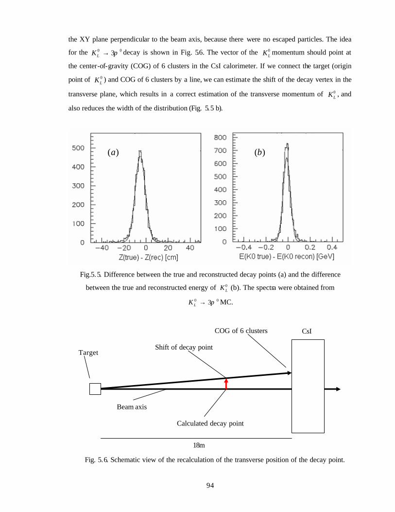
94

the XY plane perpendicular to the beam axis, because there were no escaped particles. The idea

for the 00 3π→LK decay is shown in Fig. 5.6. The vector of the 0LK momentum should point at

the center-of-gravity (COG) of 6 clusters in the CsI calorimeter. If we connect the target (origin

point of 0LK ) and COG of 6 clusters by a line, we can estimate the shift of the decay vertex in the

transverse plane, which results in a correct estimation of the transverse momentum of 0LK , and

also reduces the width of the distribution (Fig. 5.5 b).

Fig.5.5. Difference between the true and reconstructed decay points (a) and the difference

between the true and reconstructed energy of 0LK (b). The spectra were obtained from

00 3π→LK MC.

Fig. 5.6. Schematic view of the recalculation of the transverse position of the decay point.

CsI

Beam axis

Target

COG of 6 clusters

Calculated decay point

Shift of decay point

18m

)(a )(b

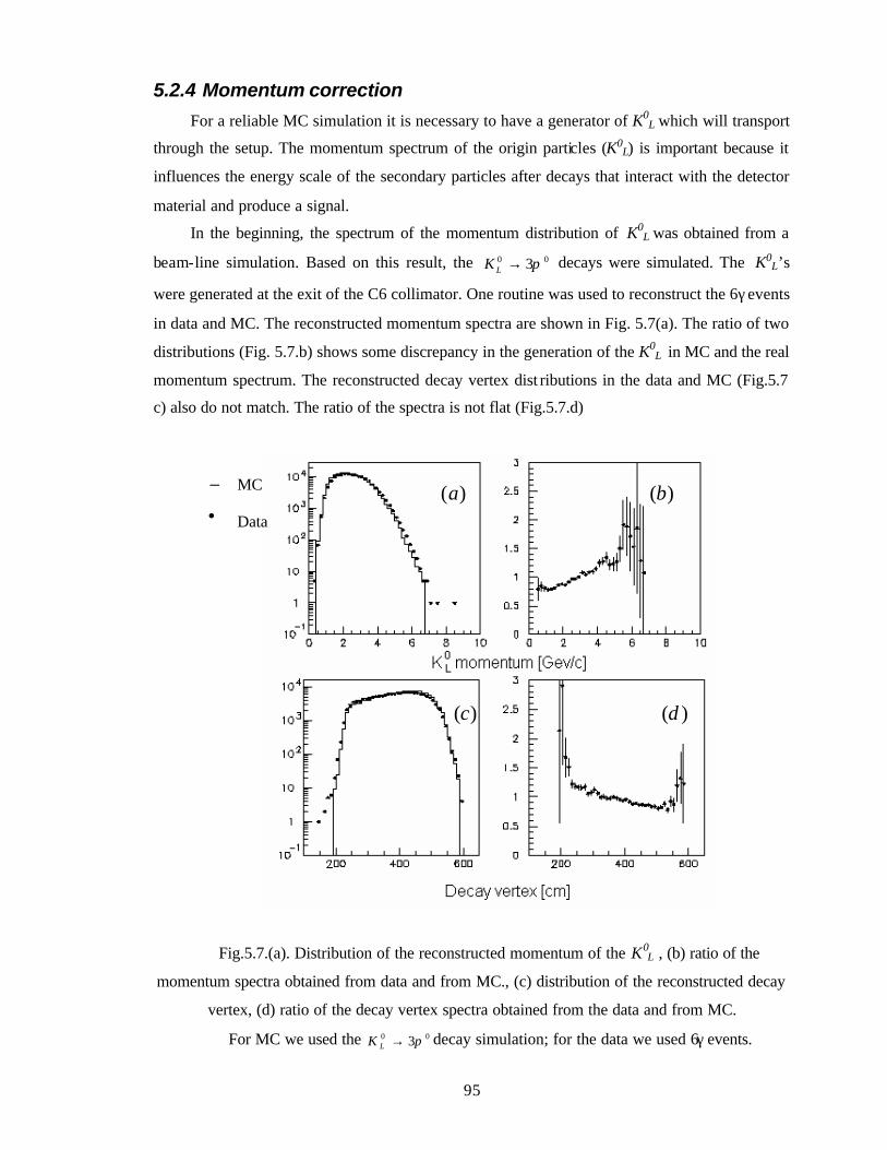
95

5.2.4 Momentum correction

For a reliable MC simulation it is necessary to have a generator of K0L which will transport

through the setup. The momentum spectrum of the origin particles (K0L) is important because it

influences the energy scale of the secondary particles after decays that interact with the detector

material and produce a signal.

In the beginning, the spectrum of the momentum distribution of K0L was obtained from a

beam-line simulation. Based on this result, the 00 3π→LK decays were simulated. The K0L’s

were generated at the exit of the C6 collimator. One routine was used to reconstruct the 6γ events

in data and MC. The reconstructed momentum spectra are shown in Fig. 5.7(a). The ratio of two

distributions (Fig. 5.7.b) shows some discrepancy in the generation of the K0L in MC and the real

momentum spectrum. The reconstructed decay vertex dist ributions in the data and MC (Fig.5.7

c) also do not match. The ratio of the spectra is not flat (Fig.5.7.d)

Fig.5.7.(a). Distribution of the reconstructed momentum of the K0L , (b) ratio of the

momentum spectra obtained from data and from MC., (c) distribution of the reconstructed decay

vertex, (d) ratio of the decay vertex spectra obtained from the data and from MC.

For MC we used the 00 3π→LK decay simulation; for the data we used 6γ events.

)(a )(b

)(c )(d

MC Data

•−

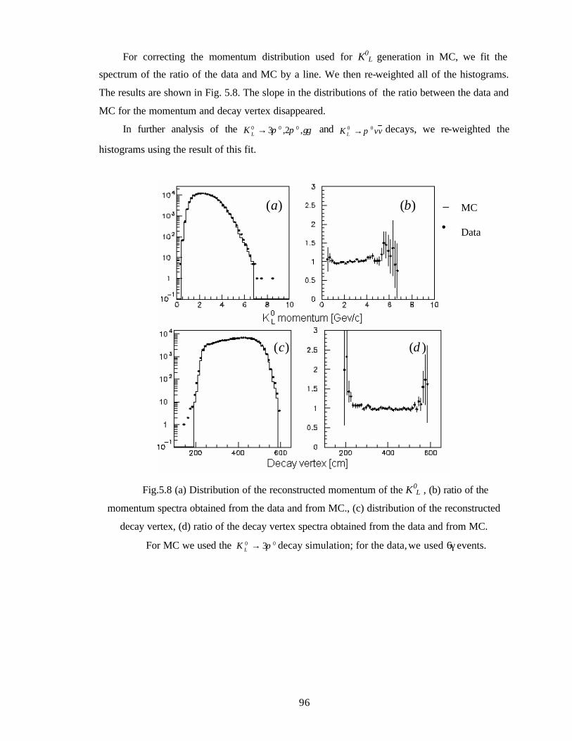
96

For correcting the momentum distribution used for K0L generation in MC, we fit the

spectrum of the ratio of the data and MC by a line. We then re-weighted all of the histograms.

The results are shown in Fig. 5.8. The slope in the distributions of the ratio between the data and

MC for the momentum and decay vertex disappeared.

In further analysis of the γγππ ,2,3 000 →LK and vvK L00 π→ decays, we re-weighted the

histograms using the result of this fit.

Fig.5.8 (a) Distribution of the reconstructed momentum of the K0L , (b) ratio of the

momentum spectra obtained from the data and from MC., (c) distribution of the reconstructed

decay vertex, (d) ratio of the decay vertex spectra obtained from the data and from MC.

For MC we used the 00 3π→LK decay simulation; for the data, we used 6γ events.

)(a )(b

)(c )(d

MC Data •

−

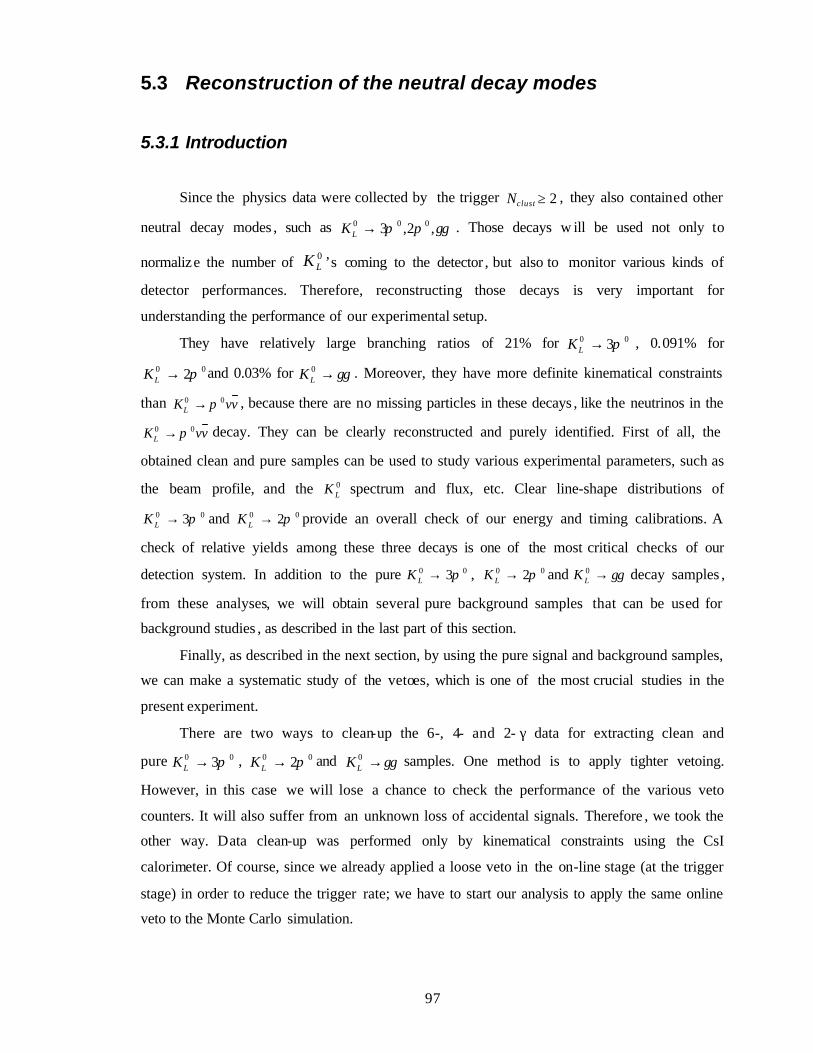
97

5.3 Reconstruction of the neutral decay modes

5.3.1 Introduction

Since the physics data were collected by the trigger 2≥clustN , they also contained other

neutral decay modes , such as γγππ ,2,3 000 →LK . Those decays w ill be used not only to

normalize the number of 0LK ’s coming to the detector , but also to monitor various kinds of

detector performances. Therefore, reconstructing those decays is very important for

understanding the performance of our experimental setup.

They have relatively large branching ratios of 21% for 00 3π→LK , 0.091% for

00 2π→LK and 0.03% for γγ→0LK . Moreover, they have more definite kinematical constraints

than vvKL00 π→ , because there are no missing particles in these decays , like the neutrinos in the

vvKL00 π→ decay. They can be clearly reconstructed and purely identified. First of all, the

obtained clean and pure samples can be used to study various experimental parameters, such as

the beam profile, and the 0LK spectrum and flux, etc. Clear line-shape distributions of

00 3π→LK and 00 2π→LK provide an overall check of our energy and timing calibrations. A

check of relative yields among these three decays is one of the most critical checks of our

detection system. In addition to the pure 00 3π→LK , 00 2π→LK and γγ→0LK decay samples ,

from these analyses, we will obtain several pure background samples that can be used for

background studies , as described in the last part of this section.

Finally, as described in the next section, by using the pure signal and background samples,

we can make a systematic study of the vetoes, which is one of the most crucial studies in the

present experiment.

There are two ways to clean-up the 6-, 4- and 2- γ data for extracting clean and

pure 00 3π→LK , 00 2π→LK and γγ→0LK samples. One method is to apply tighter vetoing.

However, in this case we will lose a chance to check the performance of the various veto

counters. It will also suffer from an unknown loss of accidental signals. Therefore , we took the

other way. Data clean-up was performed only by kinematical constraints using the CsI

calorimeter. Of course, since we already applied a loose veto in the on-line stage (at the trigger

stage) in order to reduce the trigger rate; we have to start our analysis to apply the same online

veto to the Monte Carlo simulation.

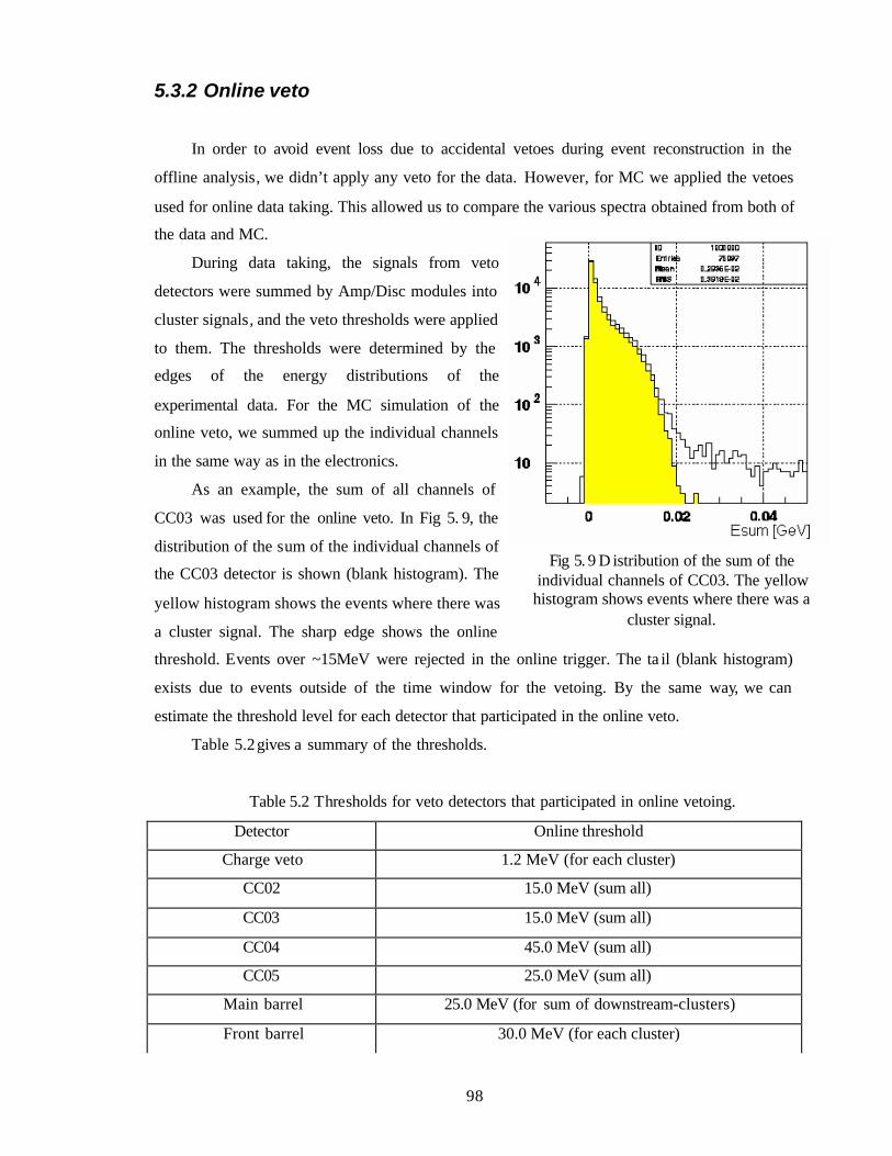
98

Fig 5. 9 D istribution of the sum of the individual channels of CC03. The yellow

histogram shows events where there was a cluster signal.

5.3.2 Online veto

In order to avoid event loss due to accidental vetoes during event reconstruction in the

offline analysis, we didn’t apply any veto for the data. However, for MC we applied the vetoes

used for online data taking. This allowed us to compare the various spectra obtained from both of

the data and MC.

During data taking, the signals from veto

detectors were summed by Amp/Disc modules into

cluster signals, and the veto thresholds were applied

to them. The thresholds were determined by the

edges of the energy distributions of the

experimental data. For the MC simulation of the

online veto, we summed up the individual channels

in the same way as in the electronics.

As an example, the sum of all channels of

CC03 was used for the online veto. In Fig 5. 9, the

distribution of the sum of the individual channels of

the CC03 detector is shown (blank histogram). The

yellow histogram shows the events where there was

a cluster signal. The sharp edge shows the online

threshold. Events over ~15MeV were rejected in the online trigger. The ta il (blank histogram)

exists due to events outside of the time window for the vetoing. By the same way, we can

estimate the threshold level for each detector that participated in the online veto.

Table 5.2 gives a summary of the thresholds.

Table 5.2 Thresholds for veto detectors that participated in online vetoing.

Detector Online threshold

Charge veto 1.2 MeV (for each cluster)

CC02 15.0 MeV (sum all)

CC03 15.0 MeV (sum all)

CC04 45.0 MeV (sum all)

CC05 25.0 MeV (sum all)

Main barrel 25.0 MeV (for sum of downstream-clusters)

Front barrel 30.0 MeV (for each cluster)

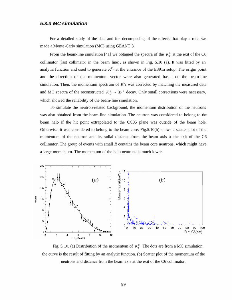
99

5.3.3 MC simulation

For a detailed study of the data and for decomposing of the effects that play a role, we

made a Monte-Carlo simulation (MC) using GEANT 3.

From the beam-line simulation [41] we obtained the spectra of the 0LK at the exit of the C6

collimator (last collimator in the beam line) , as shown in Fig. 5.10 (a). It was fitted by an

analytic function and used to generate K0L at the entrance of the E391a setup. The origin point

and the direction of the momentum vector were also generated based on the beam-line

simulation. Then, the momentum spectrum of K0L was corrected by matching the measured data

and MC spectra of the reconstructed 00 3π→LK decay. Only small corrections were necessary,

which showed the reliability of the beam-line simulation.

To simulate the neutron-related background, the momentum distribution of the neutrons

was also obtained from the beam-line simulation. The neutron was considered to belong to the

beam halo if the hit point extrapolated to the CC05 plane was outside of the beam hole.

Otherwise, it was considered to belong to the beam core. Fig.5.10(b) shows a scatter plot of the

momentum of the neutron and its radial distance from the beam axis at the exit of the C6

collimator. The group of events with small R contains the beam core neutrons, which might have

a large momentum. The momentum of the halo neutrons is much lower.

Fig. 5. 10. (a) Distribution of the momentum of 0LK . The dots are from a MC simulation;

the curve is the result of fitting by an analytic function. (b) Scatter plot of the momentum of the

neutrons and distance from the beam axis at the exit of the C6 collimator.

)(a )(b

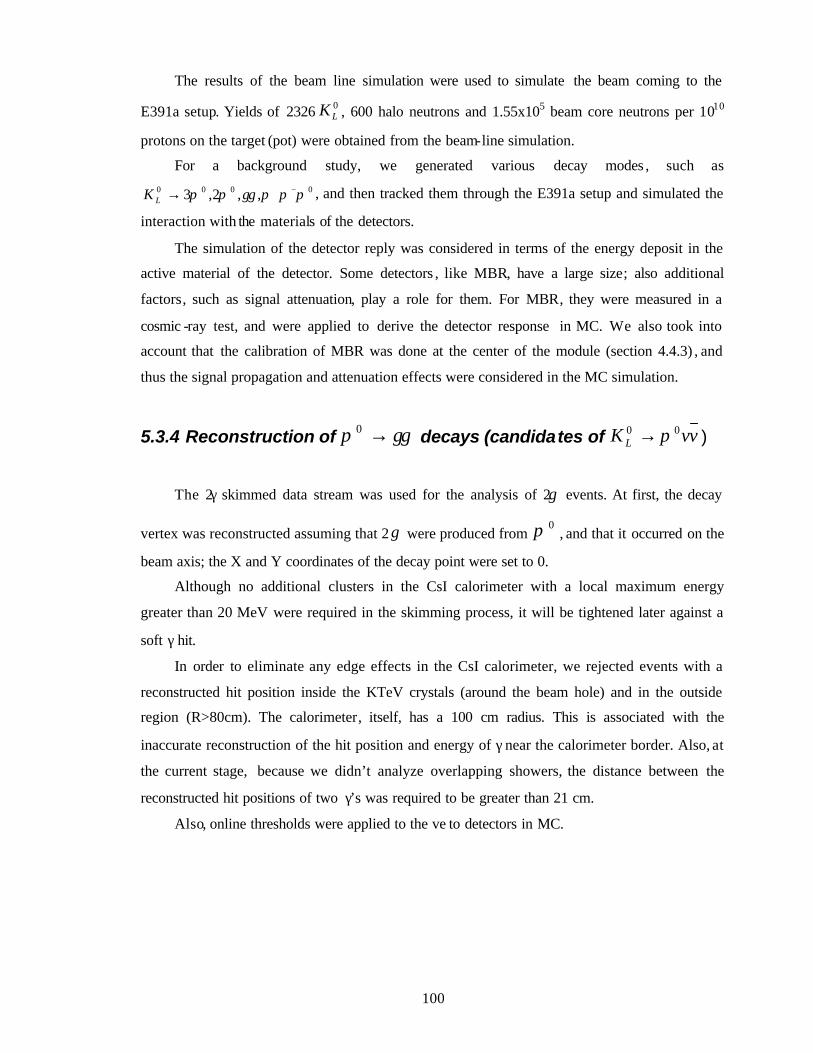
100

The results of the beam line simulation were used to simulate the beam coming to the

E391a setup. Yields of 2326 0LK , 600 halo neutrons and 1.55x105 beam core neutrons per 1010

protons on the target (pot) were obtained from the beam-line simulation.

For a background study, we generated various decay modes , such as 0000 ,,2,3 πππγγππ −+→LK , and then tracked them through the E391a setup and simulated the

interaction with the materials of the detectors.

The simulation of the detector reply was considered in terms of the energy deposit in the

active material of the detector. Some detectors , like MBR, have a large size; also additional

factors, such as signal attenuation, play a role for them. For MBR, they were measured in a

cosmic -ray test, and were applied to derive the detector response in MC. We also took into

account that the calibration of MBR was done at the center of the module (section 4.4.3) , and

thus the signal propagation and attenuation effects were considered in the MC simulation.

5.3.4 Reconstruction of γγπ →0 decays (candidates of vvK L00 π→ )

The 2γ skimmed data stream was used for the analysis of 2γ events. At first, the decay

vertex was reconstructed assuming that 2 γ were produced from 0π , and that it occurred on the

beam axis; the X and Y coordinates of the decay point were set to 0.

Although no additional clusters in the CsI calorimeter with a local maximum energy

greater than 20 MeV were required in the skimming process, it will be tightened later against a

soft γ hit.

In order to eliminate any edge effects in the CsI calorimeter, we rejected events with a

reconstructed hit position inside the KTeV crystals (around the beam hole) and in the outside

region (R>80cm). The calorimeter, itself, has a 100 cm radius. This is associated with the

inaccurate reconstruction of the hit position and energy of γ near the calorimeter border. Also, at

the current stage, because we didn’t analyze overlapping showers, the distance between the

reconstructed hit positions of two γ’s was required to be greater than 21 cm.

Also, online thresholds were applied to the ve to detectors in MC.

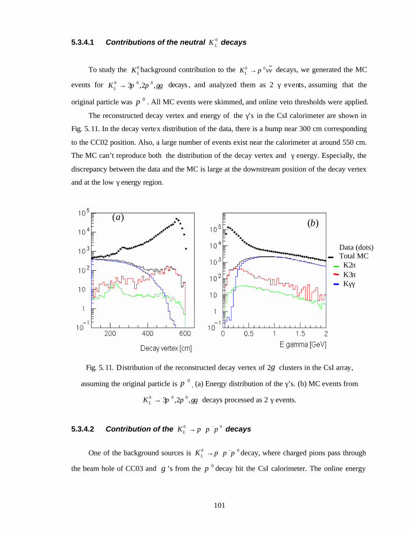
101

5.3.4.1 Contributions of the neutral 0LK decays

To study the 0LK background contribution to the vvKL

00 π→ decays, we generated the MC

events for γγππ ,2,3 000 →LK decays , and analyzed them as 2 γ events, assuming that the

original particle was 0π . All MC events were skimmed, and online veto thresholds were applied.

The reconstructed decay vertex and energy of the γ’s in the CsI calorimeter are shown in

Fig. 5. 11. In the decay vertex distribution of the data, there is a bump near 300 cm corresponding

to the CC02 position. Also, a large number of events exist near the calorimeter at around 550 cm.

The MC can’t reproduce both the distribution of the decay vertex and γ energy. Especially, the

discrepancy between the data and the MC is large at the downstream position of the decay vertex

and at the low γ energy region.

Fig. 5. 11. Distribution of the reconstructed decay vertex of 2γ clusters in the CsI array,

assuming the original particle is 0π . (a) Energy distribution of the γ’s. (b) MC events from

γγππ ,2,3 000 →LK decays processed as 2 γ events.

5.3.4.2 Contribution of the 00 πππ −+→LK decays

One of the background sources is 00 πππ −+→LK decay, where charged pions pass through

the beam hole of CC03 and γ ’s from the 0π decay hit the CsI calorimeter. The online energy

)(a)(b

Data (dots) Total MC

K2π K3π Κγγ

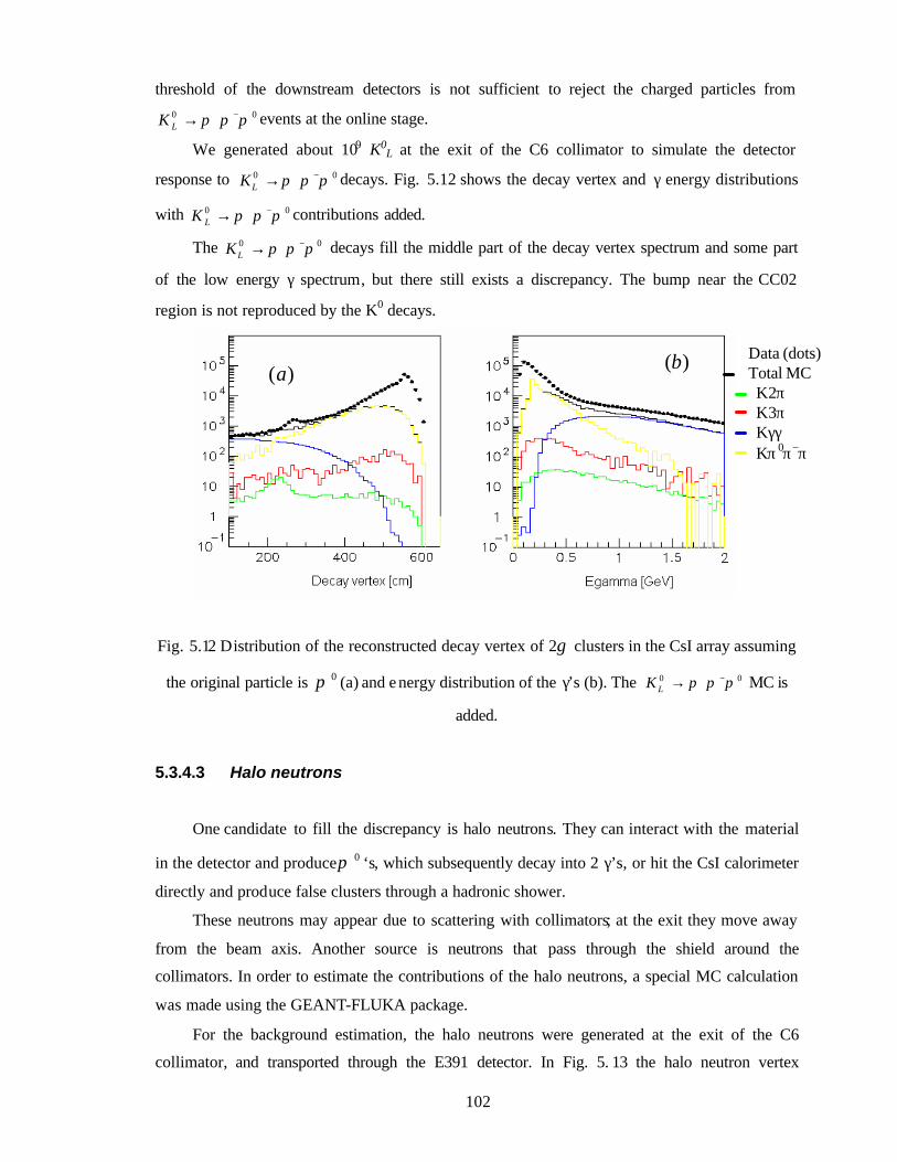
102

threshold of the downstream detectors is not sufficient to reject the charged particles from 00 πππ −+→LK events at the online stage.

We generated about 109 K0L at the exit of the C6 collimator to simulate the detector

response to 00 πππ −+→LK decays. Fig. 5.12 shows the decay vertex and γ energy distributions

with 00 πππ −+→LK contributions added.

The 00 πππ −+→LK decays fill the middle part of the decay vertex spectrum and some part

of the low energy γ spectrum, but there still exists a discrepancy. The bump near the CC02

region is not reproduced by the K0 decays.

Fig. 5.12 Distribution of the reconstructed decay vertex of 2γ clusters in the CsI array assuming

the original particle is 0π (a) and e nergy distribution of the γ’s (b). The 00 πππ −+→LK MC is

added.

5.3.4.3 Halo neutrons

One candidate to fill the discrepancy is halo neutrons. They can interact with the material

in the detector and produce 0π ‘s, which subsequently decay into 2 γ’s, or hit the CsI calorimeter

directly and produce false clusters through a hadronic shower.

These neutrons may appear due to scattering with collimators; at the exit they move away

from the beam axis. Another source is neutrons that pass through the shield around the

collimators. In order to estimate the contributions of the halo neutrons, a special MC calculation

was made using the GEANT-FLUKA package.

For the background estimation, the halo neutrons were generated at the exit of the C6

collimator, and transported through the E391 detector. In Fig. 5. 13 the halo neutron vertex

)(a )(b Data (dots) Total MC K2π K3π Κγγ Kπ 0π−π+

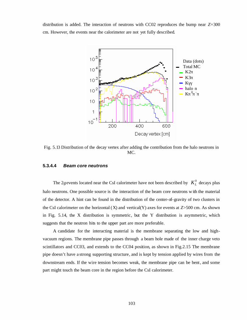
103

distribution is added. The interaction of neutrons with CC02 reproduces the bump near Z=300

cm. However, the events near the calorimeter are not yet fully described.

Fig. 5.13 Distribution of the decay vertex after adding the contribution from the halo neutrons in MC.

5.3.4.4 Beam core neutrons

The 2γ events located near the CsI calorimeter have not been described by 0LK decays plus

halo neutrons. One possible source is the interaction of the beam core neutrons w ith the material

of the detector. A hint can be found in the distribution of the center-of-gravity of two clusters in

the CsI calorimeter on the horizontal (X) and vertical(Y) axes for events at Z>500 cm. As shown

in Fig. 5.14, the X distribution is symmetric, but the Y distribution is asymmetric, which

suggests that the neutron hits to the upper part are more preferable.

A candidate for the interacting material is the membrane separating the low and high-

vacuum regions. The membrane pipe passes through a beam hole made of the inner charge veto

scintillators and CC03, and extends to the CC04 position, as shown in Fig.2.15 The membrane

pipe doesn’t have a strong supporting structure, and is kept by tension applied by wires from the

downstream ends. If the wire tension becomes weak, the membrane pipe can be bent , and some

part might touch the beam core in the region before the CsI calorimeter.

Data (dots) Total MC K2π K3π Κγγ halo n Kπ 0π−π+

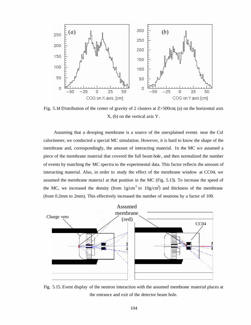
104

Fig. 5.14 Distribution of the center of gravity of 2 clusters at Z>500cm; (a) on the horizontal axis

X, (b) on the vertical axis Y .

Assuming that a drooping membrane is a source of the unexplained events near the CsI

calorimeter, we conducted a special MC simulation. However, it is hard to know the shape of the

membrane and, correspondingly, the amount of interacting material. In the MC we assumed a

piece of the membrane material that covered the full beam hole , and then normalized the number

of events by matching the MC spectra to the experimental data. This factor reflects the amount of

interacting material. Also, in order to study the effect of the membrane window at CC04, we

assumed the membrane materia l at that position in the MC (Fig. 5.15). To increase the speed of

the MC, we increased the density (from 1g/cm3 to 10g/cm3) and thickness of the membrane

(from 0.2mm to 2mm). This effectively increased the number of neutrons by a factor of 100.

Fig. 5.15. Event display of the neutron interaction with the assumed membrane material places at

the entrance and exit of the detector beam hole.

Assumed membrane

(red) CC04

Charge veto

)(a )(b

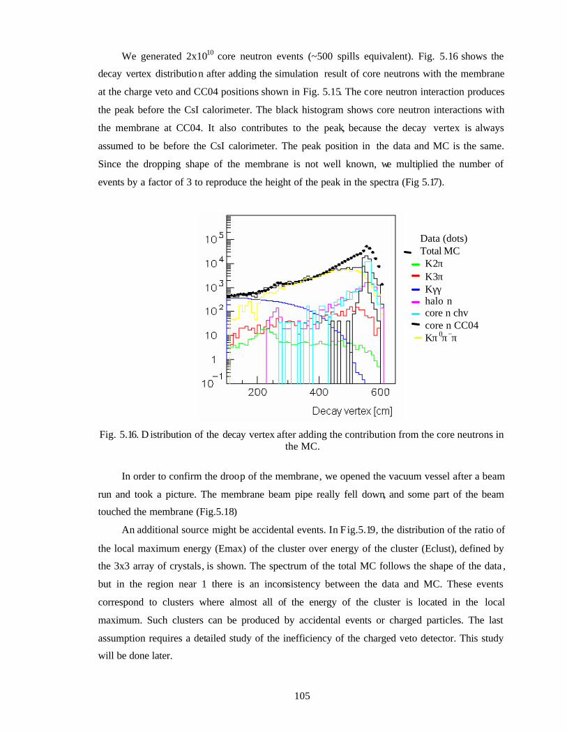
105

We generated 2x1010 core neutron events (~500 spills equivalent). Fig. 5.16 shows the

decay vertex distribution after adding the simulation result of core neutrons with the membrane

at the charge veto and CC04 positions shown in Fig. 5.15. The core neutron interaction produces

the peak before the CsI calorimeter. The black histogram shows core neutron interactions with

the membrane at CC04. It also contributes to the peak, because the decay vertex is always

assumed to be before the CsI calorimeter. The peak position in the data and MC is the same.

Since the dropping shape of the membrane is not well known, we multiplied the number of

events by a factor of 3 to reproduce the height of the peak in the spectra (Fig 5.17).

Fig. 5.16. D istribution of the decay vertex after adding the contribution from the core neutrons in the MC.

In order to confirm the droop of the membrane, we opened the vacuum vessel after a beam

run and took a picture. The membrane beam pipe really fell down, and some part of the beam

touched the membrane (Fig.5.18)

An additional source might be accidental events. In F ig.5.19, the distribution of the ratio of

the local maximum energy (Emax) of the cluster over energy of the cluster (Eclust), defined by

the 3x3 array of crystals, is shown. The spectrum of the total MC follows the shape of the data ,

but in the region near 1 there is an inconsistency between the data and MC. These events

correspond to clusters where almost all of the energy of the cluster is located in the local

maximum. Such clusters can be produced by accidental events or charged particles. The last

assumption requires a detailed study of the inefficiency of the charged veto detector. This study

will be done later.

Data (dots) Total MC K2π K3π Κγγ halo n core n chv core n CC04 Kπ 0π−π+

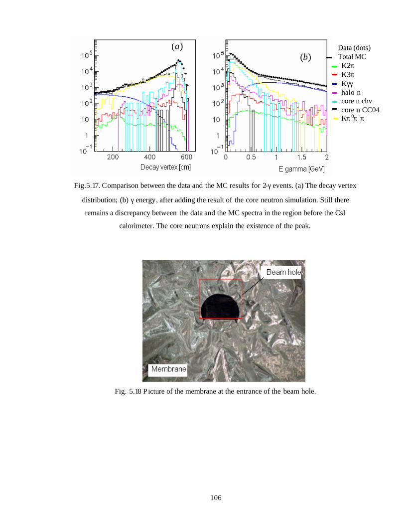
106

Fig.5.17. Comparison between the data and the MC results for 2-γ events. (a) The decay vertex

distribution; (b) γ energy, after adding the result of the core neutron simulation. Still there

remains a discrepancy between the data and the MC spectra in the region before the CsI

calorimeter. The core neutrons explain the existence of the peak.

Fig. 5.18 P icture of the membrane at the entrance of the beam hole.

)(a)(b

Data (dots) Total MC K2π K3π Κγγ halo n core n chv core n CC04 Kπ 0π−π+

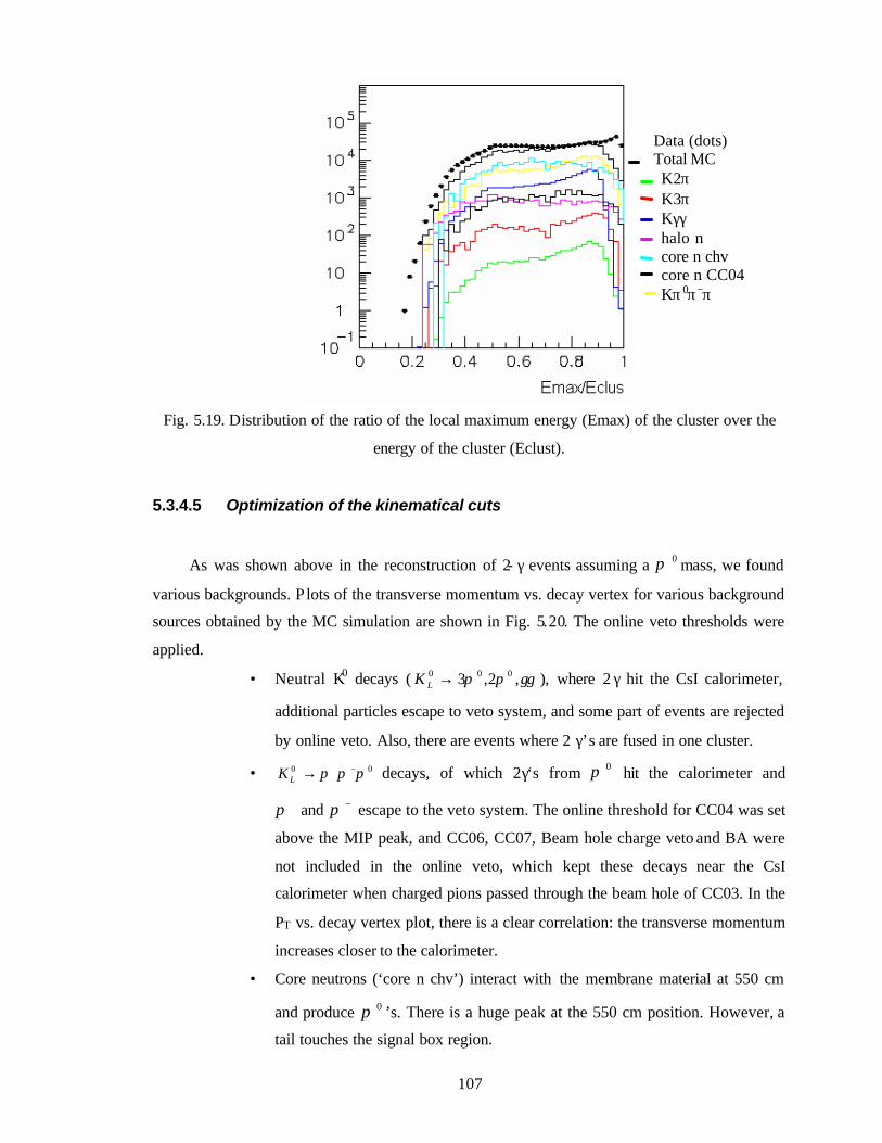
107

Fig. 5.19. Distribution of the ratio of the local maximum energy (Emax) of the cluster over the

energy of the cluster (Eclust).

5.3.4.5 Optimization of the kinematical cuts

As was shown above in the reconstruction of 2- γ events assuming a 0π mass, we found

various backgrounds. P lots of the transverse momentum vs. decay vertex for various background

sources obtained by the MC simulation are shown in Fig. 5.20. The online veto thresholds were

applied.

• Neutral K0 decays ( γγππ ,2,3 000 →LK ), where 2 γ hit the CsI calorimeter,

additional particles escape to veto system, and some part of events are rejected

by online veto. Also, there are events where 2 γ’s are fused in one cluster.

• 00 πππ −+→LK decays, of which 2γ‘s from 0π hit the calorimeter and

+π and −π escape to the veto system. The online threshold for CC04 was set

above the MIP peak, and CC06, CC07, Beam hole charge veto and BA were

not included in the online veto, which kept these decays near the CsI

calorimeter when charged pions passed through the beam hole of CC03. In the

PT vs. decay vertex plot, there is a clear correlation: the transverse momentum

increases closer to the calorimeter.

• Core neutrons (‘core n chv’) interact with the membrane material at 550 cm

and produce 0π ’s. There is a huge peak at the 550 cm position. However, a

tail touches the signal box region.

Data (dots) Total MC K2π K3π Κγγ halo n core n chv core n CC04 Kπ 0π−π+

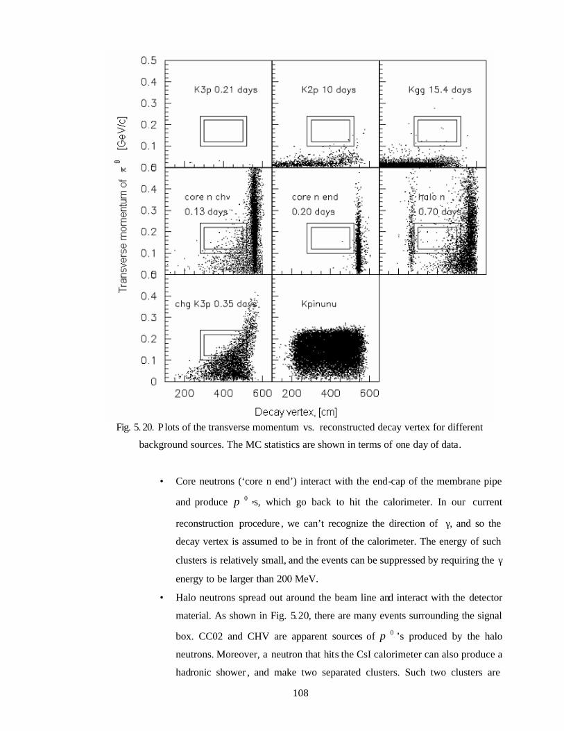
108

Fig. 5. 20. P lots of the transverse momentum vs. reconstructed decay vertex for different

background sources. The MC statistics are shown in terms of one day of data.

• Core neutrons (‘core n end’) interact with the end-cap of the membrane pipe

and produce 0π ’s, which go back to hit the calorimeter. In our current

reconstruction procedure , we can’t recognize the direction of γ, and so the

decay vertex is assumed to be in front of the calorimeter. The energy of such

clusters is relatively small, and the events can be suppressed by requiring the γ

energy to be larger than 200 MeV.

• Halo neutrons spread out around the beam line and interact with the detector

material. As shown in Fig. 5.20, there are many events surrounding the signal

box. CC02 and CHV are apparent sources of 0π ’s produced by the halo

neutrons. Moreover, a neutron that hits the CsI calorimeter can also produce a

hadronic shower , and make two separated clusters. Such two clusters are

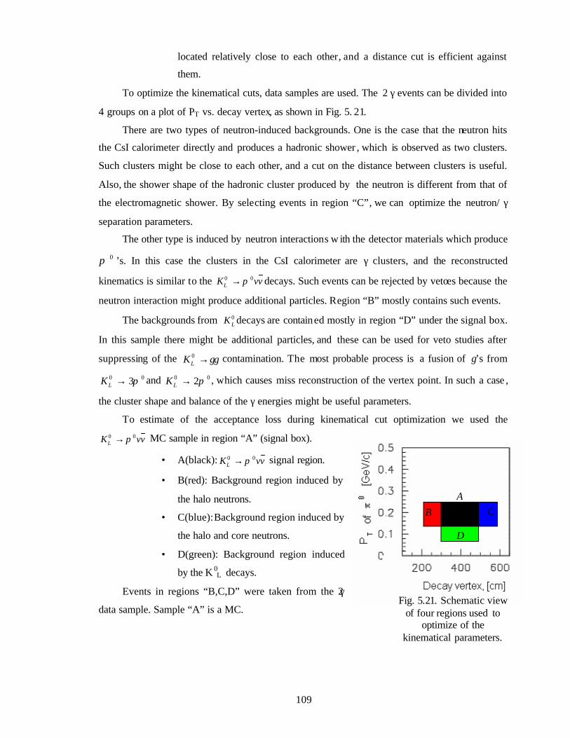
109

located relatively close to each other, and a distance cut is efficient against

them.

To optimize the kinematical cuts, data samples are used. The 2 γ events can be divided into

4 groups on a plot of PT vs. decay vertex, as shown in Fig. 5. 21.

There are two types of neutron-induced backgrounds. One is the case that the neutron hits

the CsI calorimeter directly and produces a hadronic shower , which is observed as two clusters.

Such clusters might be close to each other, and a cut on the distance between clusters is useful.

Also, the shower shape of the hadronic cluster produced by the neutron is different from that of

the electromagnetic shower. By selecting events in region “C”, we can optimize the neutron/ γ

separation parameters.

The other type is induced by neutron interactions w ith the detector materials which produce

0π ’s. In this case the clusters in the CsI calorimeter are γ clusters, and the reconstructed

kinematics is similar to the vvKL00 π→ decays. Such events can be rejected by vetoes because the

neutron interaction might produce additional particles. Region “B” mostly contains such events.

The backgrounds from 0LK decays are contained mostly in region “D” under the signal box.

In this sample there might be additional particles, and these can be used for veto studies after

suppressing of the γγ→0LK contamination. The most probable process is a fusion of γ’s from

00 3π→LK and 00 2π→LK , which causes miss reconstruction of the vertex point. In such a case ,

the cluster shape and balance of the γ energies might be useful parameters.

To estimate of the acceptance loss during kinematical cut optimization we used the

vvKL00 π→ MC sample in region “A” (signal box).

• A(black): vvKL00 π→ signal region.

• B(red): Background region induced by

the halo neutrons.

• C(blue): Background region induced by

the halo and core neutrons.

• D(green): Background region induced

by the K 0L decays.

Events in regions “B,C,D” were taken from the 2γ

data sample. Sample “A” is a MC.

Fig. 5.21. Schematic view of four regions used to

optimize of the kinematical parameters.

B CA

D

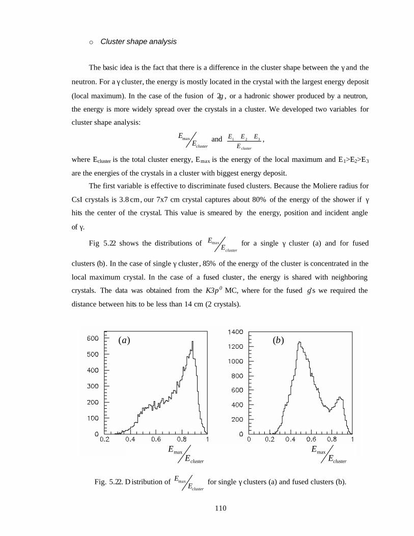
110

o Cluster shape analysis

The basic idea is the fact that there is a difference in the cluster shape between the γ and the

neutron. For a γ cluster, the energy is mostly located in the crystal with the largest energy deposit

(local maximum). In the case of the fusion of 2γ , or a hadronic shower produced by a neutron,

the energy is more widely spread over the crystals in a cluster. We developed two variables for

cluster shape analysis:

clusterEEmax and

clusterEEEE 321 ++ ,

where Ecluster is the total cluster energy, Emax is the energy of the local maximum and E1>E2>E3

are the energies of the crystals in a cluster with biggest energy deposit.

The first variable is effective to discriminate fused clusters. Because the Moliere radius for

CsI crystals is 3.8 cm, our 7x7 cm crystal captures about 80% of the energy of the shower if γ

hits the center of the crystal. This value is smeared by the energy, position and incident angle

of γ.

Fig 5.22 shows the distributions of clusterE

Emax for a single γ cluster (a) and for fused

clusters (b). In the case of single γ cluster , 85% of the energy of the cluster is concentrated in the

local maximum crystal. In the case of a fused cluster , the energy is shared with neighboring

crystals. The data was obtained from the K3π0 MC, where for the fused γ’s we required the

distance between hits to be less than 14 cm (2 crystals).

Fig. 5.22. D istribution of clusterE

Emax for single γ clusters (a) and fused clusters (b).

)(a )(b

clusterE

Emax

clusterEEmax

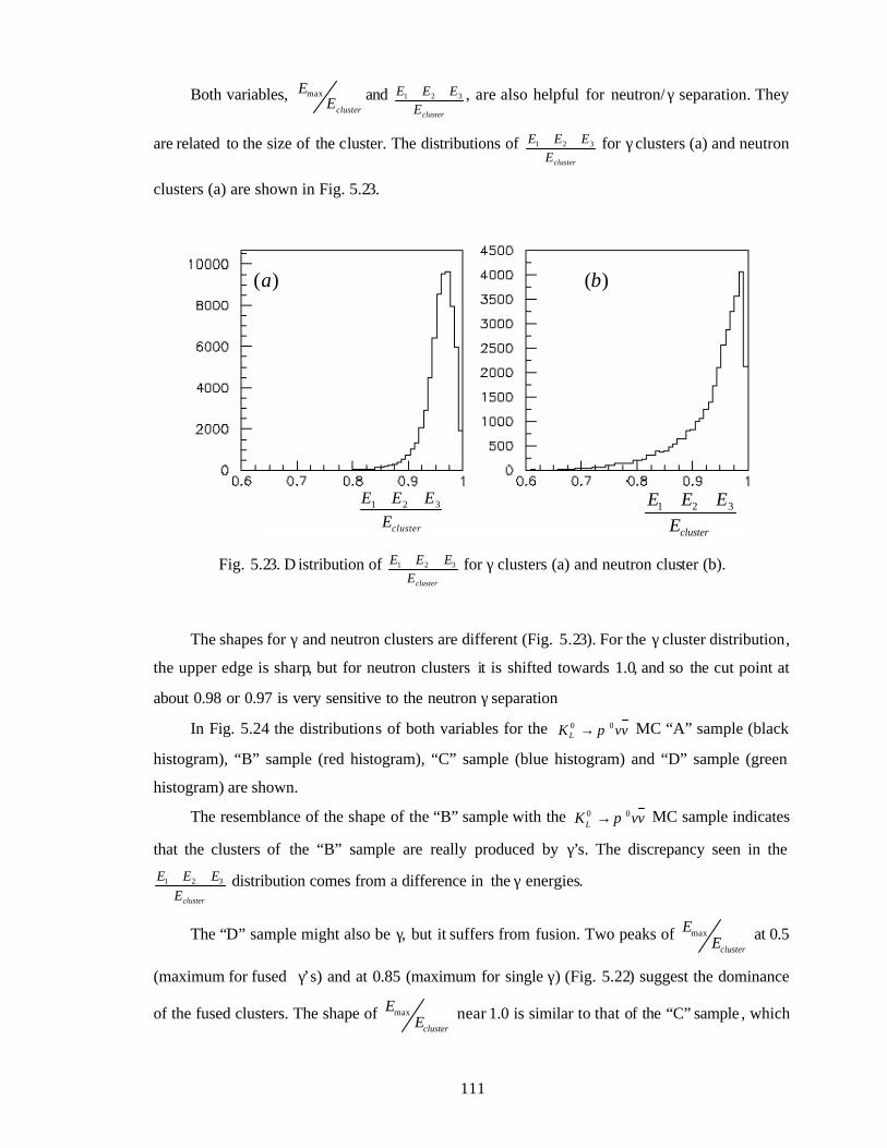
111

Both variables, clusterE

Emax and clusterE

EEE 321 ++ , are also helpful for neutron/ γ separation. They

are related to the size of the cluster. The distributions of clusterE

EEE 321 ++ for γ clusters (a) and neutron

clusters (a) are shown in Fig. 5.23.

Fig. 5.23. D istribution of clusterE

EEE 321 ++ for γ clusters (a) and neutron cluster (b).

The shapes for γ and neutron clusters are different (Fig. 5.23). For the γ cluster distribution,

the upper edge is sharp, but for neutron clusters it is shifted towards 1.0, and so the cut point at

about 0.98 or 0.97 is very sensitive to the neutron γ separation

In Fig. 5.24 the distributions of both variables for the vvKL00 π→ MC “A” sample (black

histogram), “B” sample (red histogram), “C” sample (blue histogram) and “D” sample (green

histogram) are shown.

The resemblance of the shape of the “B” sample with the vvKL00 π→ MC sample indicates

that the clusters of the “B” sample are really produced by γ’s. The discrepancy seen in the

clusterEEEE 321 ++ distribution comes from a difference in the γ energies.

The “D” sample might also be γ, but it suffers from fusion. Two peaks of clusterE

Emax at 0.5

(maximum for fused γ’s) and at 0.85 (maximum for single γ) (Fig. 5.22) suggest the dominance

of the fused clusters. The shape of clusterE

Emax near 1.0 is similar to that of the “C” sample , which

)(a )(b

clusterE

EEE 321 ++

clusterEEEE 321 ++

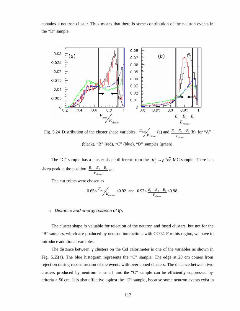
112

contains a neutron cluster. Thus means that there is some contribution of the neutron events in

the “D” sample.

Fig. 5.24. Distribution of the cluster shape variables, clusterE

Emax (a) and clusterE

EEE 321 ++ (b), for “A”

(black), “B” (red), “C” (blue), “D” samples (green).

The “C” sample has a cluster shape different from the vvKL00 π→ MC sample. There is a

sharp peak at the position 1321 =++

clusterEEEE .

The cut points were chosen as

0.65<clusterE

Emax <0.92 and 0.92<clusterE

EEE 321 ++ <0.98.

o Distance and energy balance of ?γ’s

The cluster shape is valuable for rejection of the neutron and fused clusters, but not for the

“B” samples, which are produced by neutron interactions with CC02. For this region, we have to

introduce additional variables.

The distance between γ clusters on the CsI calorimeter is one of the variables as shown in

Fig. 5.25(a). The blue histogram represents the “C” sample. The edge at 20 cm comes from

rejection during reconstruction of the events with overlapped clusters. The distance between two

clusters produced by neutrons is small, and the “C” sample can be efficiently suppressed by

criteria > 50 cm. It is also effective against the “D” sample , because some neutron events exist in

)(a )(b

clusterE

EEE 321 ++clusterE

Emax

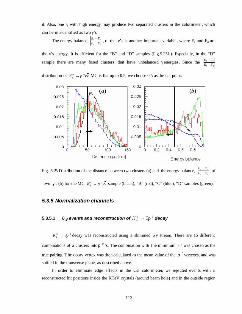
113

it. Also, one γ with high energy may produce two separated clusters in the calorimeter, which

can be misidentified as two γ’s.

The energy balance, 21

21

EEEE

+− , of the γ’s is another important variable, where E1 and E2 are

the γ’s energy. It is efficient for the “B” and “D” samples (Fig.5.25.b). Especially, in the “D”

sample there are many fused clusters that have unbalanced γ energies. Since the 21

21

EEEE

+−

distribution of vvKL00 π→ MC is flat up to 0.5, we choose 0.5 as the cut point.

Fig. 5.25 Distribution of the distance between two clusters (a) and the energy balance, 21

21

EEEE

+−

, of

two γ’s (b) for the MC vvKL00 π→ sample (black), “B” (red), “C” (blue), “D” samples (green).

5.3.5 Normalization channels

5.3.5.1 6 γ events and reconstruction of 00 3π→LK decay

00 3π→LK decay was reconstructed using a skimmed 6 γ stream. There are 15 different

combinations of a clusters into 0π ’s. The combination with the minimum 2χ was chosen as the

true pairing. The decay vertex was then calculated as the mean value of the 0π vertexes, and was

shifted in the transverse plane , as described above.

In order to eliminate edge effects in the CsI calorimeter, we rejected events with a

reconstructed hit positions inside the KTeV crystals (around beam hole) and in the outside region

)(a )(b

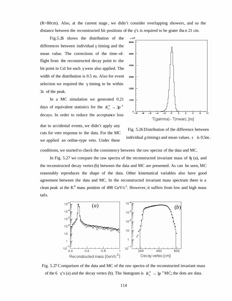
114

Fig. 5.26 Distribution of the difference between

individual γ timings and mean values. σ is 0.5ns.

(R>80cm). Also, at the current stage , we didn’t consider overlapping showers, and so the

distance between the reconstructed hit positions of the γ’s is required to be grater tha n 21 cm.

Fig.5.26 shows the distribution of the

differences between individual γ timing and the

mean value. The corrections of the time-of-

flight from the reconstructed decay point to the

hit point in CsI for each γ were also applied. The

width of the distribution is 0.5 ns. Also for event

selection we required the γ timing to be within

3σ of the peak.

In a MC simulation we generated 0.21

days of equivalent statistics for the 00 3π→LK decays. In order to reduce the acceptance loss

due to accidental events, we didn’t apply any

cuts for veto response to the data. For the MC

we applied an online-type veto. Under these

conditions, we started to check the consistency between the raw spectra of the data and MC.

In Fig. 5.27 we compare the raw spectra of the reconstructed invariant mass of 6γ (a), and

the reconstructed decay vertex (b) between the data and MC are presented. As can be seen, MC

reasonably reproduces the shape of the data. Other kinematical variables also have good

agreement between the data and MC. In the reconstructed invariant mass spectrum there is a

clean peak at the K0 mass position of 498 GeV/c2. However, it suffers from low and high mass

tails.

Fig. 5.27 C omparison of the data and MC of the raw spectra of the reconstructed invariant mass

of the 6 γ’s (a) and the decay vertex (b). The histogram is 00 3π→LK MC; the dots are data.

)(a )(b

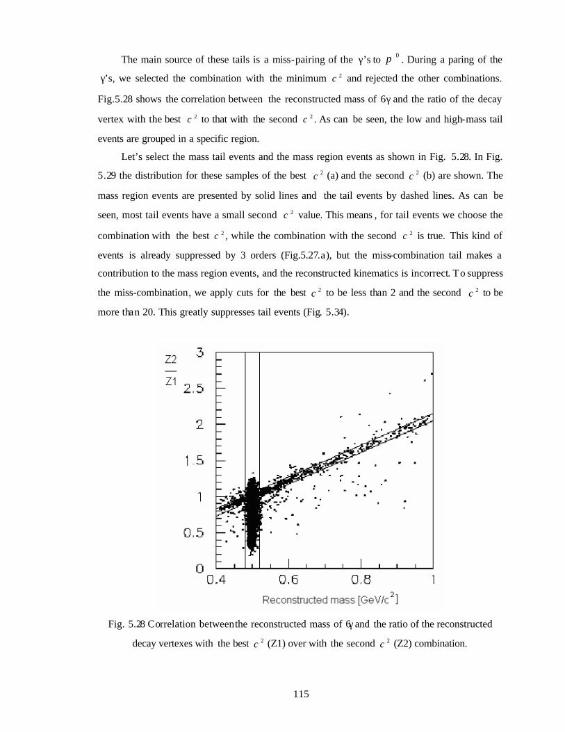
115

The main source of these tails is a miss-pairing of the γ’s to 0π . During a paring of the

γ’s, we selected the combination with the minimum 2χ and rejected the other combinations.

Fig.5.28 shows the correlation between the reconstructed mass of 6γ and the ratio of the decay

vertex with the best 2χ to that with the second 2χ . As can be seen, the low and high-mass tail

events are grouped in a specific region.

Let’s select the mass tail events and the mass region events as shown in Fig. 5.28. In Fig.

5.29 the distribution for these samples of the best 2χ (a) and the second 2χ (b) are shown. The

mass region events are presented by solid lines and the tail events by dashed lines. As can be

seen, most tail events have a small second 2χ value. This means , for tail events we choose the

combination with the best 2χ , while the combination with the second 2χ is true. This kind of

events is already suppressed by 3 orders (Fig.5.27.a), but the miss-combination tail makes a

contribution to the mass region events, and the reconstructed kinematics is incorrect. To suppress

the miss-combination, we apply cuts for the best 2χ to be less than 2 and the second 2χ to be

more than 20. This greatly suppresses tail events (Fig. 5.34).

Fig. 5.28 Correlation between the reconstructed mass of 6γ and the ratio of the reconstructed

decay vertexes with the best 2χ (Z1) over with the second 2χ (Z2) combination.

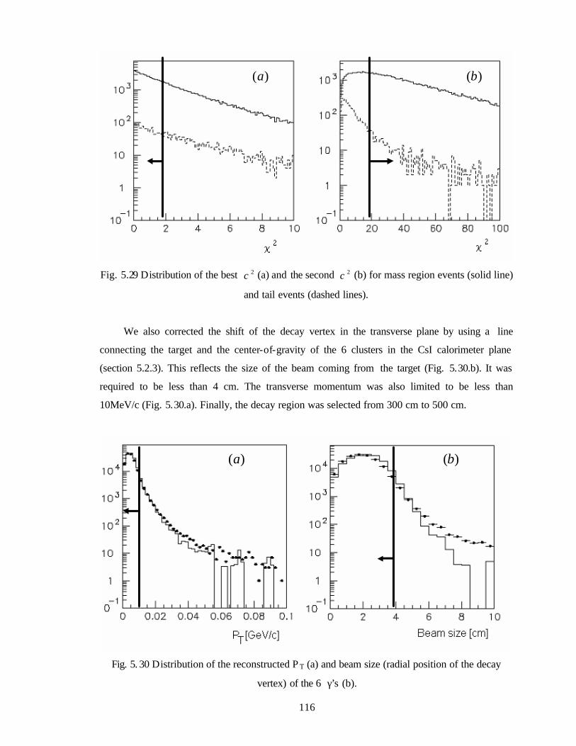
116

Fig. 5.29 Distribution of the best 2χ (a) and the second 2χ (b) for mass region events (solid line)

and tail events (dashed lines).

We also corrected the shift of the decay vertex in the transverse plane by using a line

connecting the target and the center-of-gravity of the 6 clusters in the CsI calorimeter plane

(section 5.2.3). This reflects the size of the beam coming from the target (Fig. 5.30.b). It was

required to be less than 4 cm. The transverse momentum was also limited to be less than

10MeV/c (Fig. 5.30.a). Finally, the decay region was selected from 300 cm to 500 cm.

Fig. 5. 30 Distribution of the reconstructed P T (a) and beam size (radial position of the decay

vertex) of the 6 γ’s (b).

)(a )(b

)(a )(b

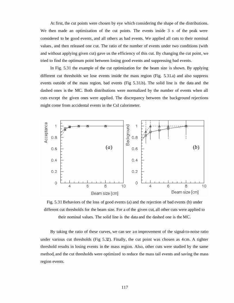
117

At first, the cut points were chosen by eye which considering the shape of the distributions.

We then made an optimization of the cut points. The events inside 3 σ of the peak were

considered to be good events, and all others as bad events. We applied all cuts to their nominal

values , and then released one cut. The ratio of the number of events under two conditions (with

and without applying given cut) gave us the efficiency of this cut. By changing the cut point, we

tried to find the optimum point between losing good events and suppressing bad events.

In Fig. 5.31 the example of the cut optimization for the beam size is shown. By applying

different cut thresholds we lose events inside the mass region (Fig. 5.31.a) and also suppress

events outside of the mass region, bad events (Fig 5.31.b). The solid line is the data and the

dashed ones is the MC. Both distributions were normalized by the number of events when all

cuts except the given ones were applied. The discrepancy between the background rejections

might come from accidental events in the CsI calorimeter.

Fig. 5.31 Behaviors of the loss of good events (a) and the rejection of bad events (b) under

different cut thresholds for the beam size. For a of the given cut, all other cuts were applied to

their nominal values. The solid line is the data and the dashed one is the MC.

By taking the ratio of these curves, we can see an improvement of the signal-to-noise ratio

under various cut thresholds (Fig 5.32). Finally, the cut point was chosen as 4 cm. A tighter

threshold results in losing events in the mass region. Also, other cuts were studied by the same

method, and the cut thresholds were optimized to reduce the mass tail events and saving the mass

region events.

)(a )(b

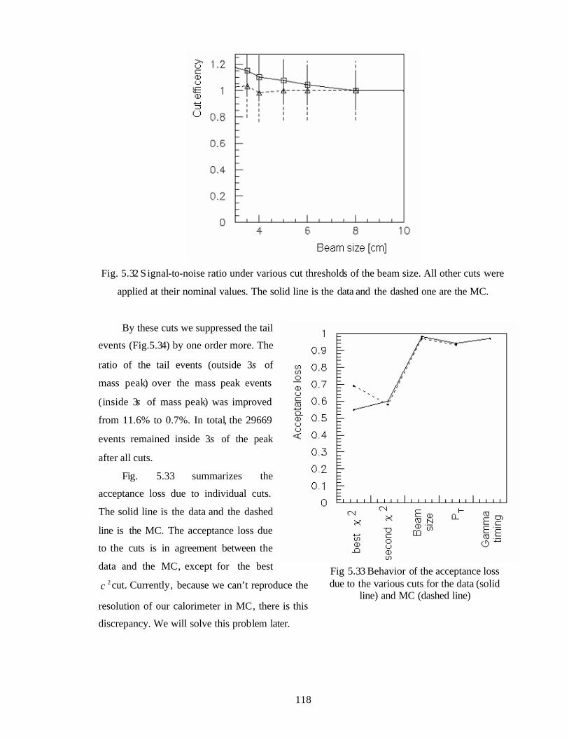
118

Fig 5.33 Behavior of the acceptance loss due to the various cuts for the data (solid

line) and MC (dashed line)

Fig. 5.32 S ignal-to-noise ratio under various cut thresholds of the beam size. All other cuts were

applied at their nominal values. The solid line is the data and the dashed one are the MC.

By these cuts we suppressed the tail

events (Fig.5.34) by one order more. The

ratio of the tail events (outside 3σ of

mass peak) over the mass peak events

(inside 3σ of mass peak) was improved

from 11.6% to 0.7%. In total, the 29669

events remained inside 3σ of the peak

after all cuts.

Fig. 5.33 summarizes the

acceptance loss due to individual cuts.

The solid line is the data and the dashed

line is the MC. The acceptance loss due

to the cuts is in agreement between the

data and the MC, except for the best 2χ cut. Currently, because we can’t reproduce the

resolution of our calorimeter in MC, there is this

discrepancy. We will solve this problem later.

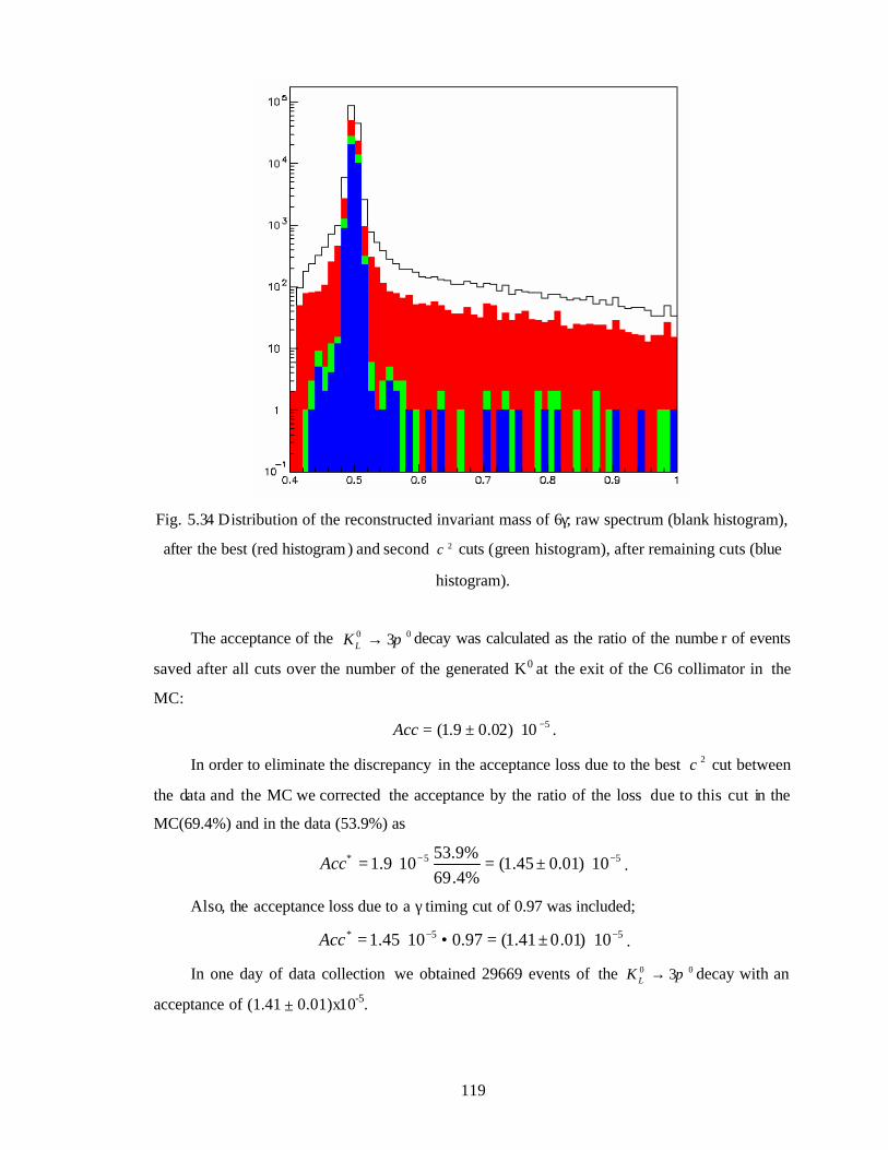
119

Fig. 5.34 Distribution of the reconstructed invariant mass of 6γ; raw spectrum (blank histogram),

after the best (red histogram) and second 2χ cuts (green histogram), after remaining cuts (blue

histogram).

The acceptance of the 00 3π→LK decay was calculated as the ratio of the numbe r of events

saved after all cuts over the number of the generated K0 at the exit of the C6 collimator in the

MC: 510)02.09.1( −⋅±=Acc .

In order to eliminate the discrepancy in the acceptance loss due to the best 2χ cut between

the data and the MC we corrected the acceptance by the ratio of the loss due to this cut in the

MC(69.4%) and in the data (53.9%) as

55* 10)01.045.1(%4.69%9.53

109.1 −− ⋅±=⋅=Acc .

Also, the acceptance loss due to a γ timing cut of 0.97 was included;

55* 10)01.041.1(97.01045.1 −− ⋅±=•⋅=Acc .

In one day of data collection we obtained 29669 events of the 00 3π→LK decay with an

acceptance of (1.41 ± 0.01)x10-5.

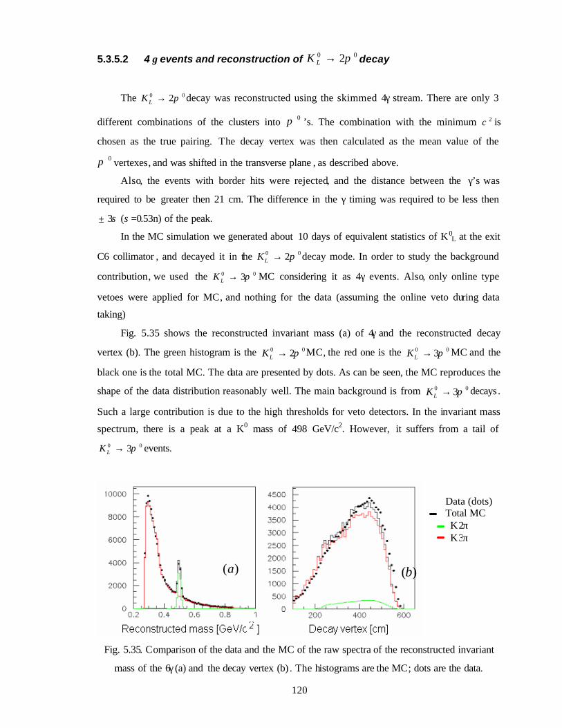
120

5.3.5.2 4 γ events and reconstruction of 00 2π→LK decay

The 00 2π→LK decay was reconstructed using the skimmed 4γ stream. There are only 3

different combinations of the clusters into 0π ’s. The combination with the minimum 2χ is

chosen as the true pairing. The decay vertex was then calculated as the mean value of the

0π vertexes, and was shifted in the transverse plane , as described above.

Also, the events with border hits were rejected, and the distance between the γ’s was

required to be greater then 21 cm. The difference in the γ timing was required to be less then

± 3σ (σ=0.53n) of the peak.

In the MC simulation we generated about 10 days of equivalent statistics of K0L at the exit

C6 collimator , and decayed it in the 00 2π→LK decay mode. In order to study the background

contribution, we used the 00 3π→LK MC considering it as 4γ events. Also, only online type

vetoes were applied for MC, and nothing for the data (assuming the online veto during data

taking)

Fig. 5.35 shows the reconstructed invariant mass (a) of 4γ and the reconstructed decay

vertex (b). The green histogram is the 00 2π→LK MC, the red one is the 00 3π→LK MC and the

black one is the total MC. The data are presented by dots. As can be seen, the MC reproduces the

shape of the data distribution reasonably well. The main background is from 00 3π→LK decays.

Such a large contribution is due to the high thresholds for veto detectors. In the invariant mass

spectrum, there is a peak at a K0 mass of 498 GeV/c2. However, it suffers from a tail of 00 3π→LK events.

Fig. 5.35. Comparison of the data and the MC of the raw spectra of the reconstructed invariant

mass of the 6γ (a) and the decay vertex (b) . The histograms are the MC; dots are the data.

)(a )(b

Data (dots) Total MC K2π K3π

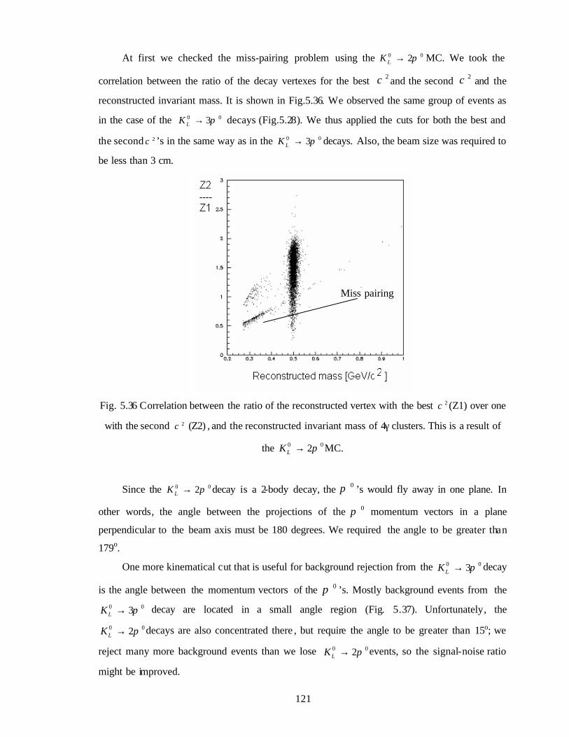
121

At first we checked the miss-pairing problem using the 00 2π→LK MC. We took the

correlation between the ratio of the decay vertexes for the best 2χ and the second 2χ and the

reconstructed invariant mass. It is shown in Fig.5.36. We observed the same group of events as

in the case of the 00 3π→LK decays (Fig.5.28). We thus applied the cuts for both the best and

the second 2χ ’s in the same way as in the 00 3π→LK decays. Also, the beam size was required to

be less than 3 cm.

Fig. 5.36 Correlation between the ratio of the reconstructed vertex with the best 2χ (Z1) over one

with the second 2χ (Z2) , and the reconstructed invariant mass of 4γ clusters. This is a result of

the 00 2π→LK MC.

Since the 00 2π→LK decay is a 2-body decay, the 0π ’s would fly away in one plane. In

other words, the angle between the projections of the 0π momentum vectors in a plane

perpendicular to the beam axis must be 180 degrees. We required the angle to be greater than

179o.

One more kinematical cut that is useful for background rejection from the 00 3π→LK decay

is the angle between the momentum vectors of the 0π ’s. Mostly background events from the 00 3π→LK decay are located in a small angle region (Fig. 5.37). Unfortunately, the

00 2π→LK decays are also concentrated there , but require the angle to be greater than 15o; we

reject many more background events than we lose 00 2π→LK events, so the signal-noise ratio

might be improved.

Miss pairing

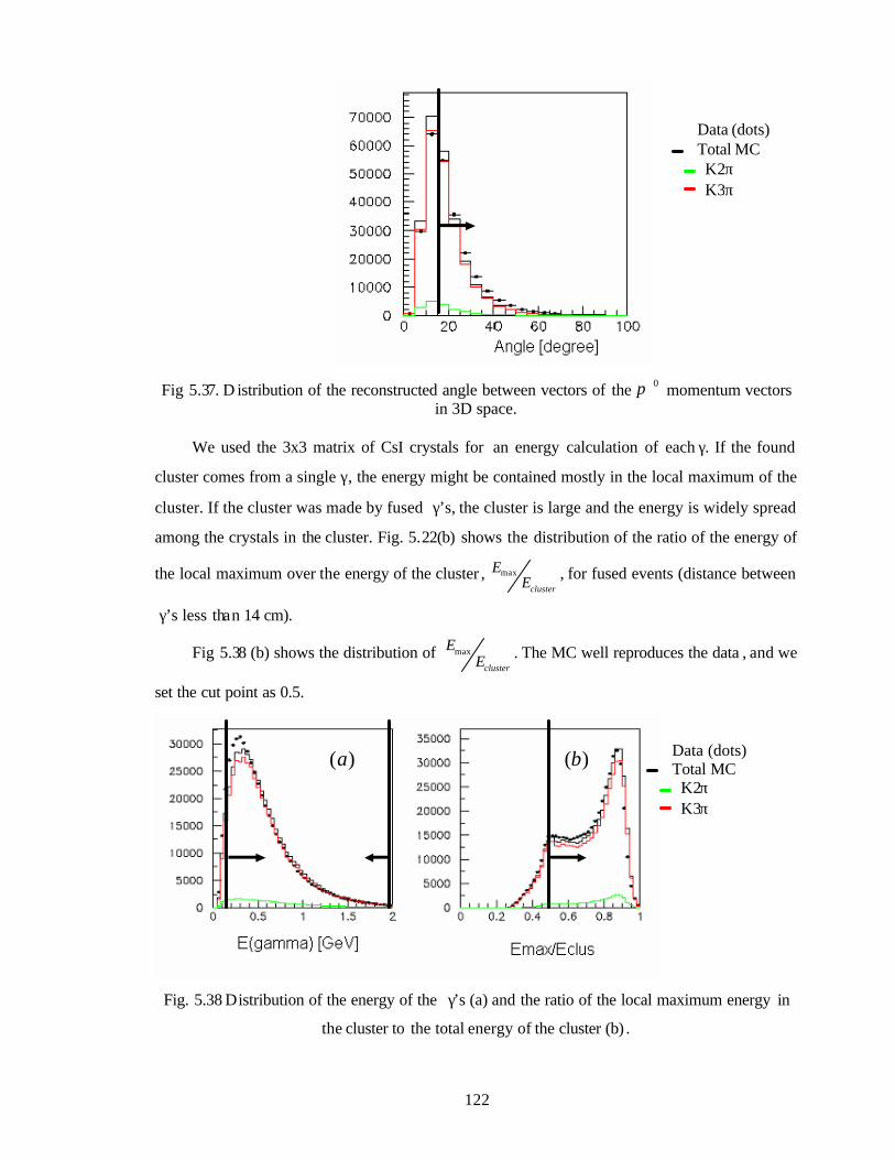
122

Fig 5.37. D istribution of the reconstructed angle between vectors of the 0π momentum vectors in 3D space.

We used the 3x3 matrix of CsI crystals for an energy calculation of each γ. If the found

cluster comes from a single γ, the energy might be contained mostly in the local maximum of the

cluster. If the cluster was made by fused γ’s, the cluster is large and the energy is widely spread

among the crystals in the cluster. Fig. 5.22(b) shows the distribution of the ratio of the energy of

the local maximum over the energy of the cluster , clusterE

Emax , for fused events (distance between

γ’s less than 14 cm).

Fig 5.38 (b) shows the distribution of clusterE

Emax . The MC well reproduces the data , and we

set the cut point as 0.5.

Fig. 5.38 Distribution of the energy of the γ’s (a) and the ratio of the local maximum energy in

the cluster to the total energy of the cluster (b) .

Data (dots) Total MC K2π K3π

)(a )(b Data (dots) Total MC

K2π K3π

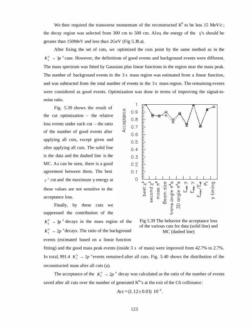
123

Fig 5.39 The behavior the acceptance loss of the various cuts for data (solid line) and

MC (dashed line)

We then required the transverse momentum of the reconstructed K0 to be less 15 MeV/c ;

the decay region was selected from 300 cm to 500 cm. Also, the energy of the γ’s should be

greater than 150MeV and less than 2GeV (Fig 5.38.a).

After fixing the set of cuts, we optimized the cuts point by the same method as in the 00 3π→LK case. However, the definitions of good events and background events were different.

The mass spectrum was fitted by Gaussian plus linear functions in the region near the mass peak.

The number of background events in the 3 σ mass region was estimated from a linear function,

and was subtracted from the total number of events in the 3 σ mass region. The remaining events

were considered as good events. Optimization was done in terms of improving the signal-to-

noise ratio.

Fig. 5.39 shows the result of

the cut optimization – the relative

loss events under each cut – the ratio

of the number of good events after

applying all cuts, except given and

after applying all cuts. The solid line

is the data and the dashed line is the

MC. As can be seen, there is a good

agreement between them. The best 2χ cut and the maximum γ energy at

these values are not sensitive to the

acceptance loss.

Finally, by these cuts we

suppressed the contribution of the 00 3π→LK decays in the mass region of the

00 2π→LK decays. The ratio of the background

events (estimated based on a linear function

fitting) and the good mass peak events (inside 3 σ of mass) were improved from 42.7% to 2.7%.

In total, 991.4 00 2π→LK events remained after all cuts. Fig. 5.40 shows the distribution of the

reconstructed mass after all cuts (a).

The acceptance of the 00 2π→LK decay was calculated as the ratio of the number of events

saved after all cuts over the number of generated K0’s at the exit of the C6 collimator: 410)01.012.1( −⋅±=Acc .

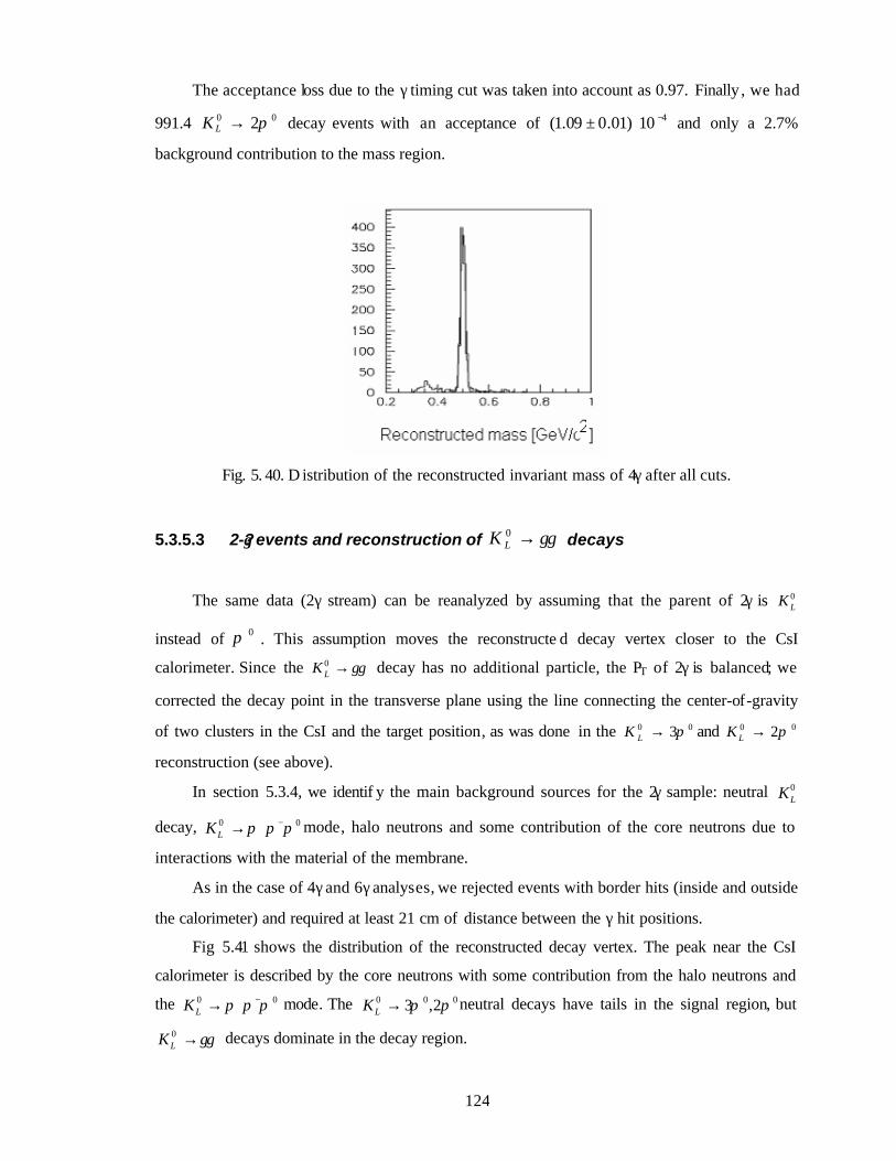
124

The acceptance loss due to the γ timing cut was taken into account as 0.97. Finally , we had

991.4 00 2π→LK decay events with an acceptance of 410)01.009.1( −⋅± and only a 2.7%

background contribution to the mass region.

Fig. 5. 40. D istribution of the reconstructed invariant mass of 4γ after all cuts.

5.3.5.3 2-?γ events and reconstruction of γγ→0LK decays

The same data (2γ stream) can be reanalyzed by assuming that the parent of 2γ is 0LK

instead of 0π . This assumption moves the reconstructe d decay vertex closer to the CsI

calorimeter. Since the γγ→0LK decay has no additional particle, the PT of 2γ is balanced; we

corrected the decay point in the transverse plane using the line connecting the center-of-gravity

of two clusters in the CsI and the target position, as was done in the 00 3π→LK and 00 2π→LK

reconstruction (see above).

In section 5.3.4, we identif y the main background sources for the 2γ sample: neutral 0LK

decay, 00 πππ −+→LK mode, halo neutrons and some contribution of the core neutrons due to

interactions with the material of the membrane.

As in the case of 4γ and 6γ analyses, we rejected events with border hits (inside and outside

the calorimeter) and required at least 21 cm of distance between the γ hit positions.

Fig 5.41 shows the distribution of the reconstructed decay vertex. The peak near the CsI

calorimeter is described by the core neutrons with some contribution from the halo neutrons and

the 00 πππ −+→LK mode. The 000 2,3 ππ→LK neutral decays have tails in the signal region, but

γγ→0LK decays dominate in the decay region.

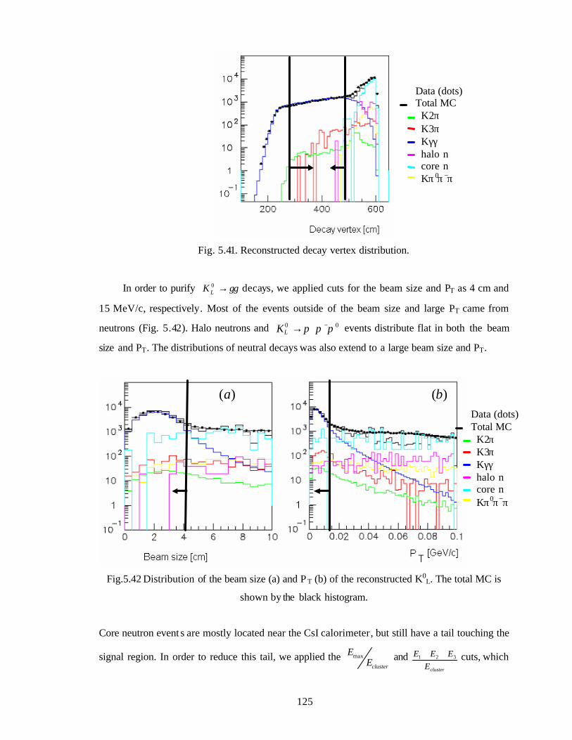
125

Fig. 5.41. Reconstructed decay vertex distribution.

In order to purify γγ→0LK decays, we applied cuts for the beam size and PT as 4 cm and

15 MeV/c, respectively. Most of the events outside of the beam size and large PT came from

neutrons (Fig. 5.42). Halo neutrons and 00 πππ −+→LK events distribute flat in both the beam

size and PT. The distributions of neutral decays was also extend to a large beam size and PT.

Fig.5.42 Distribution of the beam size (a) and P T (b) of the reconstructed K0

L. The total MC is

shown by the black histogram.

Core neutron event s are mostly located near the CsI calorimeter, but still have a tail touching the

signal region. In order to reduce this tail, we applied the clusterE

Emax

and

clusterEEEE 321 ++ cuts, which

)(a )(b

Data (dots) Total MC

K2π K3π Κγγ halo n core n Kπ 0π −π +

Data (dots) Total MC

K2π K3π Κγγ halo n core n Kπ0π−π +

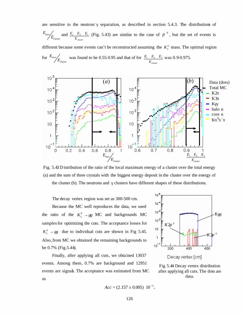
126

Fig 5.44 Decay vertex distribution after applying all cuts. The dots are

data.

are sensitive to the neutron/ γ separation, as described in section 5.4.3. The distributions of

clusterEEmax and

clusterEEEE 321 ++ (Fig. 5.43) are similar to the case of 0π , but the set of events is

different because some events can’t be reconstructed assuming the 0LK mass. The optimal region

for clusterE

Emax was found to be 0.55-0.95 and that of for clusterE

EEE 321 ++ was 0.9-0.975.

Fig. 5.43 D istribution of the ratio of the local maximum energy of a cluster over the total energy

(a) and the sum of three crystals with the biggest energy deposit in the cluster over the energy of

the cluster (b). The neutrons and γ clusters have different shapes of these distributions.

The decay vertex region was set as 300-500 cm.

Because the MC well reproduces the data, we used

the ratio of the γγ→0LK MC and backgrounds MC

samples for optimizing the cuts. The acceptance losses for

γγ→0LK due to individual cuts are shown in Fig 5.45.

Also, from MC we obtained the remaining backgrounds to

be 0.7% (Fig.5.44).

Finally, after applying all cuts, we obta ined 13037

events. Among them, 0.7% are background and 12951

events are signals. The acceptance was estimated from MC

as 310)005.0157.2( −⋅±=Acc ,

03πK

02πK

γγK

)(a )(b

clusterE

EEE 321 ++

clusterEEmax

Data (dots) Total MC

K2π K3π Κγγ halo n core n Kπ0π−π+

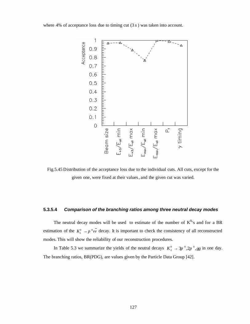
127

where 4% of acceptance loss due to timing cut (3 σ) was taken into account.

Fig.5.45 Distribution of the acceptance loss due to the individual cuts. All cuts, except for the

given one, were fixed at their values , and the given cut was varied.

5.3.5.4 Comparison of the branching ratios among three neutral decay modes

The neutral decay modes will be used to estimate of the number of K0‘s and for a BR

estimation of the vvKL00 π→ decay. It is important to check the consistency of all reconstructed

modes. This will show the reliability of our reconstruction procedures.

In Table 5.3 we summarize the yields of the neutral decays γγππ ,2,3 000 →LK in one day.

The branching ratios, BR(PDG), are values given by the Particle Data Group [42].

128

Table 5.3 Summary of the reconstructed neutral K0L decays.

00 3π→LK 00 2π→LK γγ→0LK

BR(PDG) 21.13% 9.27x10-4 5.86x10-4

Number of reconstructed events

(background are subtracted) 29669 991.4 12951

Acceptance 1.41x10-5 1.09x10-4 2.157x10-3

Backgrounds contribution 2.7% 0.7%

Number of K0L (N*) 0.99x1010 0.98x1010 1.02x1010

The number of events, N*, which are normalized by the acceptance and the branching ratio ,

reflects the number of K0‘s coming to the setup. This number should not depend on the decay

mode.

It is found that the yields of all three decay modes agree with each other within 4%, which

is within the statistical errors.

5.4 Study of the veto counters

One of the background sources to the vvKL00 π→ decay is other K0 decays, where 2γ hit

the CsI calorimeter, and other particles hit the veto counters. Since the additional particles take

away the transverse momentum, it results in fake events of vvK L00 π→ if they are undetected.

Such events can not be killed by kinematical cuts, and must be suppressed by the veto counters.

In the E391 setup, the veto and the CsI calorimeter cover almost full 4π geometry. The

calorimeter also plays the role of vetoes against additional clusters. They are suppressed by a

skimming process , but it is still necessary to take care of soft γ’s, which escaped the above

process. We thus made a study and optimization of the veto counters and the calorimeter used as

a veto.

04.002.1)3()2(

)2()3(

)3()2(

)2()3(

0

0

0

0

0

0

0*

0*

±==ππ

ππ

ππ

ππ

KAccKAcc

KNKN

KBRKBR

KNKN

04.096.0)()2(

*

0*

±=γγπ

KNKN

02.097.0)()3(

*

0*

±=γγπ

KNKN

129

5.4.1 Pure signal and background samples ( γγππ ,2,3 000 →LK )

To estimate the acceptance loss due to veto cuts, it is useful to prepare clean data samples

of the decay process without any additional particles. The data sample must be purified without

touching the veto by applying only the kinematical cuts. If the purity of the sample is high

enough, the reduction of events due to the veto is equal to the acceptance loss. Also, by applying

all veto cuts we can estimate the total acceptance loss due to the veto.

On the other hand, an event sample having additional particles is always a pure background

sample, which may be used to estimate background rejection by the veto.

In a veto study, the timing information is also crucial. It can be used to separate between

direct hits of real additional particles and shower leakage effects appearing in a veto detector. It

greatly helps to avoid the acceptance loss.

We thus have prepared pure sample s of the 00 3π→LK , 00 2π→LK and γγ→0LK decays .

They were purified only by kinematical cuts. No tighter veto than the online veto was applied.

The background contaminations for 00 3π→LK , 00 2π→LK (2.7%) and γγ→0LK (0.7%) samples

were negligibly small, and the numbers of events in these samples were about 30k, 1k and 13k,

respectively.

To study the background structure in the veto detectors, we must prepare pure samples of

events having additional particles. One of the pure background samples is a cluster of events

below the 0LK mass peak in the 4γ invariant mass distribution, which is shown in Fig. 5.35(a).

The mass distribution is well reproduced by 00 3π→LK MC, where only 4 clusters are identified

in the CsI calorimeter out of 6γ from 00 3π→LK . The other background sample, which we can

prepare, is events in the γγ→0LK sample with a decay vertex greater than 500 cm (Fig.5.41) ,

and with PT greater than 15MeV/c (Fig. 5.42.a). In this region the backgrounds from 0LK decays

and neutrons are concentrated and the contamination of the γγ→0LK decay is suppressed.

The differences in the energy and timing distributions of the veto counters between pure

signal and background samples can be used for background structure identification. The time

windows for the vetoing might be selected only for those events that must be rejected without

touching the shower leakage region. In this way we can reject background events without losing

the acceptance for signal events. Also, because we concentrated the rejection only in the direct

hit timing region, the acceptance loss is mostly due to accidental events. This means that all 3

pure signal samples must show the same acceptance loss.

130

For veto optimization we used a “D” sample of 2γ events (Fig. 5.21). As shown in Fig. 5.20,

the events from 00 3π→LK , 00 2π→LK and 00 πππ −+→LK decays are mostly located in the “D”

region. After removing γγ→0LK decays that have no additional particles, by selecting a large

acoplanarity angle, events in the “D” region can be defined as a background sample. K inematical

cuts, which are described in previous section, are also applied in order to reduce the neutron

events.

We can thus prepare three signal samples to estimate of the acceptance loss and the

background sample (region “D”) to study background rejection. By taking the ratio of events

reduction for these signal and background samples as a function of the veto threshold, we can

obtain the Figure-of-Merit of a given cut.

For a veto study it is very important to check the correlation between the energy deposit

and the hit timing of the veto detectors for both the signal and background samples. Setting the

time window for the veto is another important step in the veto study in order to keep the

acceptance for the signal.

5.4.2 Veto study of each detector

The procedure for the study of the veto detector is as follows:

• Study the correlation between the energy deposit and the hit timing for the

signal and background samples and set the time window for the veto.

• Apply the various cuts for the energy deposit and calculate the acceptance loss

using signal samples.

• The background rejection is estimated form the event loss of the “D” sample.

• Define the Figure-of-Merit and select the optimum point for the energy

threshold.

5.4.2.1 Main barrel (MBR)

The main barrel is the main detector for a veto. It has the biggest aperture, and is most

important for background rejection. The main barrel covers the decay region before the CsI

calorimeter , and also some part of the CsI calorimeter, in order to prevent the particles that hit

the edge of the calorimeter to escape .

Fig. 5.46 shows the correlation between the mean and the difference of the timings of the

downstream and upstream PMT’s for the inner modules. In those plots the large values of

T(down)-T(up) and Tmean mean the upstream hit and the later timing, respectively. Figures

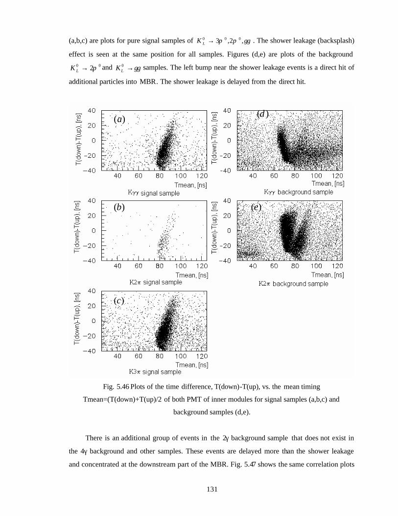
131

(a,b,c) are plots for pure signal samples of γγππ ,2,3 000 →LK . The shower leakage (backsplash)

effect is seen at the same position for all samples. Figures (d,e) are plots of the background 00 2π→LK and γγ→0

LK samples. The left bump near the shower leakage events is a direct hit of

additional particles into MBR. The shower leakage is delayed from the direct hit.

Fig. 5.46 Plots of the time difference, T(down)-T(up), vs. the mean timing

Tmean=(T(down)+T(up)/2 of both PMT of inner modules for signal samples (a,b,c) and

background samples (d,e).

There is an additional group of events in the 2γ background sample that does not exist in

the 4γ background and other samples. These events are delayed more than the shower leakage

and concentrated at the downstream part of the MBR. Fig. 5.47 shows the same correlation plots

)(a

)(b

)(c

)(d

)(e

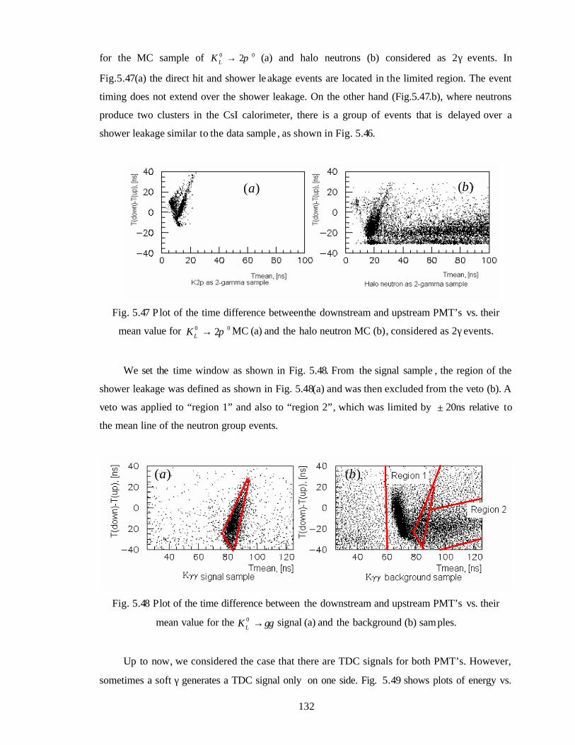
132

for the MC sample of 00 2π→LK (a) and halo neutrons (b) considered as 2γ events. In

Fig.5.47(a) the direct hit and shower le akage events are located in the limited region. The event

timing does not extend over the shower leakage. On the other hand (Fig.5.47.b), where neutrons

produce two clusters in the CsI calorimeter, there is a group of events that is delayed over a

shower leakage similar to the data sample , as shown in Fig. 5.46.

Fig. 5.47 P lot of the time difference between the downstream and upstream PMT’s vs. their

mean value for 00 2π→LK MC (a) and the halo neutron MC (b), considered as 2γ events.

We set the time window as shown in Fig. 5.48. From the signal sample , the region of the

shower leakage was defined as shown in Fig. 5.48(a) and was then excluded from the veto (b). A

veto was applied to “region 1” and also to “region 2”, which was limited by ± 20ns relative to

the mean line of the neutron group events.

Fig. 5.48 Plot of the time difference between the downstream and upstream PMT’s vs. their

mean value for the γγ→0LK signal (a) and the background (b) samples.

Up to now, we considered the case that there are TDC signals for both PMT’s. However,

sometimes a soft γ generates a TDC signal only on one side. Fig. 5.49 shows plots of energy vs.

)(a )(b

)(a )(b

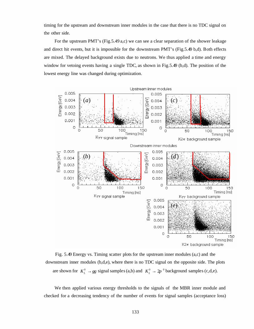
133

timing for the upstream and downstream inner modules in the case that there is no TDC signal on

the other side.

For the upstream PMT’s (Fig.5.49 a,c) we can see a clear separation of the shower leakage

and direct hit events, but it is impossible for the downstream PMT’s (Fig.5.49 b,d). Both effects

are mixed. The delayed background exists due to neutrons. We thus applied a time and energy

window for vetoing events having a single TDC, as shown in Fig.5.49 (b,d). The position of the

lowest energy line was changed during optimization.

Fig. 5.49 Energy vs. Timing scatter plots for the upstream inner modules (a,c) and the

downstream inner modules (b,d,e), where there is no TDC signal on the opposite side. The plots

are shown for γγ→0LK signal samples (a,b) and 00 2π→LK background samples (c,d,e).

We then applied various energy thresholds to the signals of the MBR inner module and

checked for a decreasing tendency of the number of events for signal samples (acceptance loss)

)(a

)(b

)(c

)(d

)(e

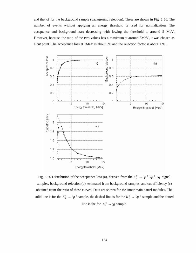
134

and that of for the background sample (background rejection). These are shown in Fig. 5. 50. The

number of events without applying an energy threshold is used for normalization. The

acceptance and background start decreasing with lowing the threshold to around 5 MeV.

However, because the ratio of the two values has a maximum at around 3MeV , it was chosen as

a cut point. The acceptance loss at 3MeV is about 5% and the rejection factor is about 10%.

Fig. 5.50 Distribution of the acceptance loss (a), derived from the γγππ ,2,3 000 →LK signal

samples, background rejection (b), estimated from background samples, and cut efficiency (c)

obtained from the ratio of these curves. Data are shown for the inner main barrel modules. The

solid line is for the 00 3π→LK sample, the dashed line is for the 00 2π→LK sample and the dotted

line is the for γγ→0LK sample.

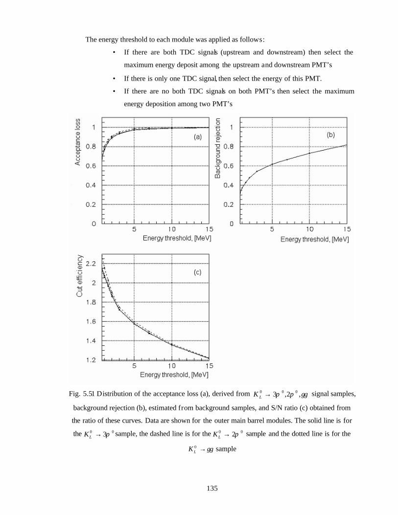
135

The energy threshold to each module was applied as follows:

• If there are both TDC signals (upstream and downstream) then select the

maximum energy deposit among the upstream and downstream PMT’s

• If there is only one TDC signal, then select the energy of this PMT.

• If there are no both TDC signals on both PMT’s then select the maximum

energy deposition among two PMT’s

Fig. 5.51 Distribution of the acceptance loss (a), derived from γγππ ,2,3 000 →LK signal samples,

background rejection (b), estimated from background samples, and S/N ratio (c) obtained from

the ratio of these curves. Data are shown for the outer main barrel modules. The solid line is for

the 00 3π→LK sample, the dashed line is for the 00 2π→LK sample and the dotted line is for the

γγ→0LK sample

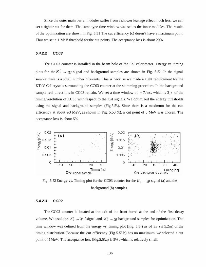
136

Since the outer main barrel modules suffer from a shower leakage effect much less, we can

set a tighter cut for them. The same type time window was set as the inner modules. The results

of the optimization are shown in Fig. 5.51 The cut efficiency (c) doesn’t have a maximum point.

Thus we set a 1 MeV threshold for the cut points. The acceptance loss is about 20%.

5.4.2.2 CC03

The CC03 counter is installed in the beam hole of the CsI calorimeter. Energy vs. timing

plots for the γγ→0LK signal and background samples are shown in Fig. 5.52. In the signal

sample there is a small number of events. This is because we made a tight requirement for the

KTeV CsI crystals surrounding the CC03 counter at the skimming procedure. In the background

sample real direct hits in CC03 remain. We set a time window of ± 7.4ns , which is 3 σ of the

timing resolution of CC03 with respect to the CsI signals. We optimized the energy thresholds

using the signal and background samples (Fig.5.53). Since there is a maximum for the cut

efficiency at about 2-3 MeV, as shown in Fig. 5.53 (b), a cut point of 3 MeV was chosen. The

acceptance loss is about 5%.

Fig. 5.52 Energy vs. Timing plot for the CC03 counter for the γγ→0LK signal (a) and the

background (b) samples.

5.4.2.3 CC02

The CC02 counter is located at the exit of the front barrel at the end of the first decay

volume. We used the 00 3π→LK signal and γγ→0LK background samples for optimization. The

time window was defined from the energy vs. timing plot (Fig. 5.54) as of 3 σ ( ± 5.2ns) of the

timing distribution. Because the cut efficiency (Fig.5.55.b) has no maximum, we selected a cut

point of 1MeV. The acceptance loss (Fig.5.55.a) is 5% , which is relatively small.

)(a )(b

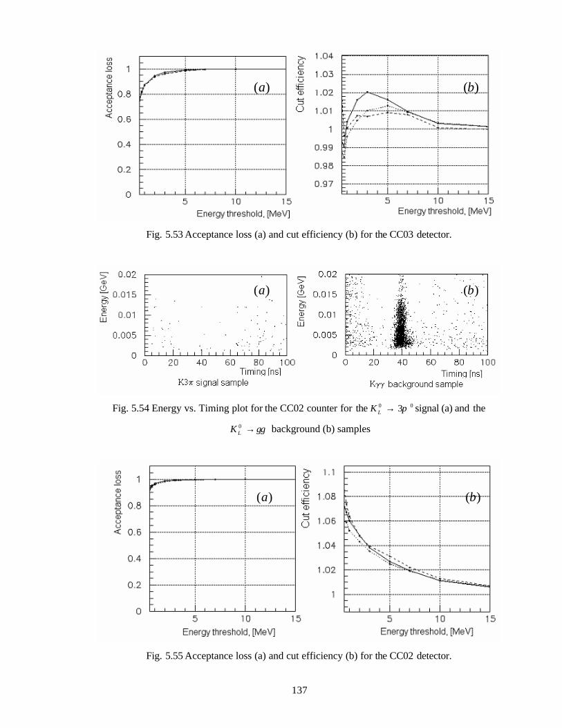
137

Fig. 5.53 Acceptance loss (a) and cut efficiency (b) for the CC03 detector.

Fig. 5.54 Energy vs. Timing plot for the CC02 counter for the 00 3π→LK signal (a) and the

γγ→0LK background (b) samples

Fig. 5.55 Acceptance loss (a) and cut efficiency (b) for the CC02 detector.

)(a )(b

)(a )(b

)(a )(b

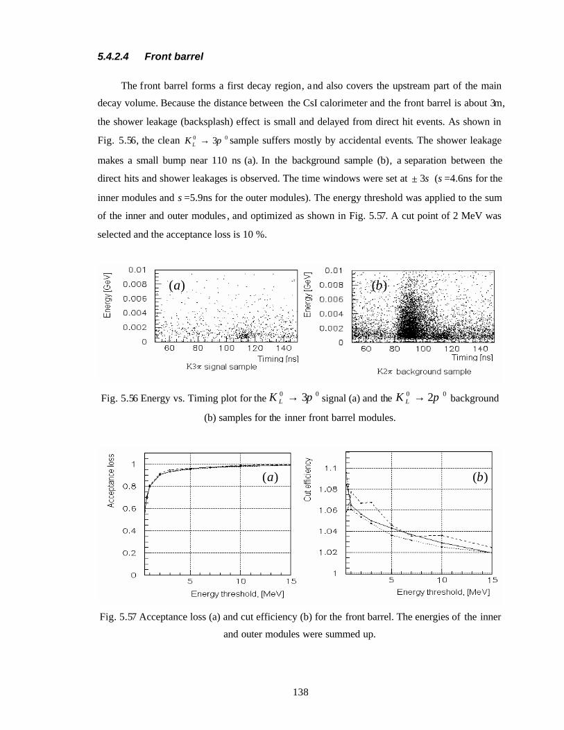
138

5.4.2.4 Front barrel

The front barrel forms a first decay region, and also covers the upstream part of the main

decay volume. Because the distance between the CsI calorimeter and the front barrel is about 3m,

the shower leakage (backsplash) effect is small and delayed from direct hit events. As shown in

Fig. 5.56, the clean 00 3π→LK sample suffers mostly by accidental events. The shower leakage

makes a small bump near 110 ns (a). In the background sample (b), a separation between the

direct hits and shower leakages is observed. The time windows were set at ± 3σ (σ=4.6ns for the

inner modules and σ=5.9ns for the outer modules). The energy threshold was applied to the sum

of the inner and outer modules , and optimized as shown in Fig. 5.57. A cut point of 2 MeV was

selected and the acceptance loss is 10 %.

Fig. 5.56 Energy vs. Timing plot for the 00 3π→LK signal (a) and the 00 2π→LK background

(b) samples for the inner front barrel modules.

Fig. 5.57 Acceptance loss (a) and cut efficiency (b) for the front barrel. The energies of the inner

and outer modules were summed up.

)(a )(b

)(a )(b

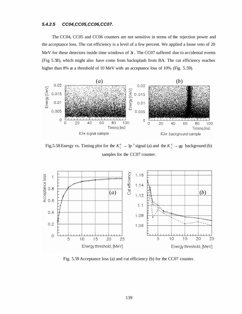
139

5.4.2.5 CC04,CC05,CC06,CC07.

The CC04, CC05 and CC06 counters are not sensitive in terms of the rejection power and

the acceptance loss. The cut efficiency is a level of a few percent. We applied a loose veto of 20

MeV for these detectors inside time windows of 3σ. The CC07 suffered due to accidental events

(Fig 5.58), which might also have come from backsplash from BA. The cut efficiency reaches

higher than 8% at a threshold of 10 MeV with an acceptance loss of 10% (Fig. 5.59).

Fig.5.58 Energy vs. Timing plot for the 00 3π→LK signal (a) and the γγ→0LK background (b)

samples for the CC07 counter.

Fig. 5.59 Acceptance loss (a) and cut efficiency (b) for the CC07 counter.

)(a)(b

)(a )(b

)(b

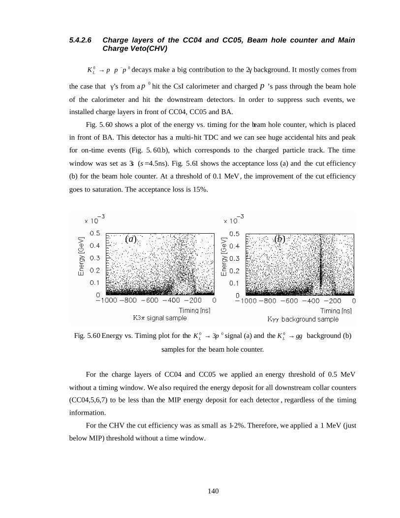
140

5.4.2.6 Charge layers of the CC04 and CC05, Beam hole counter and Main Charge Veto(CHV)

00 πππ −+→LK decays make a big contribution to the 2γ background. It mostly comes from

the case that γ’s from a 0π hit the CsI calorimeter and charged π ’s pass through the beam hole

of the calorimeter and hit the downstream detectors. In order to suppress such events, we

installed charge layers in front of CC04, CC05 and BA.

Fig. 5.60 shows a plot of the energy vs. timing for the beam hole counter, which is placed

in front of BA. This detector has a multi-hit TDC and we can see huge accidental hits and peak

for on-time events (Fig. 5. 60.b), which corresponds to the charged particle track. The time

window was set as 3σ (σ=4.5ns). Fig. 5.61 shows the acceptance loss (a) and the cut efficiency

(b) for the beam hole counter. At a threshold of 0.1 MeV, the improvement of the cut efficiency

goes to saturation. The acceptance loss is 15%.

Fig. 5.60 Energy vs. Timing plot for the 00 3π→LK signal (a) and the γγ→0LK background (b)

samples for the beam hole counter.

For the charge layers of CC04 and CC05 we applied an energy threshold of 0.5 MeV

without a timing window. We also required the energy deposit for all downstream collar counters

(CC04,5,6,7) to be less than the MIP energy deposit for each detector , regardless of the timing

information.

For the CHV the cut efficiency was as small as 1-2%. Therefore, we applied a 1 MeV (just

below MIP) threshold without a time window.

)(a )(b

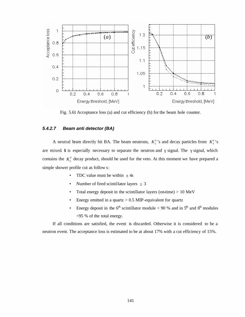
141

Fig. 5.61 Acceptance loss (a) and cut efficiency (b) for the beam hole counter.

5.4.2.7 Beam anti detector (BA)

A neutral beam directly hit BA. The beam neutrons, 0LK ’s and decay particles from 0

LK ‘s

are mixed. It is especially necessary to separate the neutron and γ signal. The γ signal, which

contains the 0LK decay product, should be used for the veto. At this moment we have prepared a

simple shower profile cut as follow s:

• TDC value must be within ± 4σ

• Number of fired scintillator layers ≥ 3

• Total energy deposit in the scintillator layers (on-time) > 10 MeV

• Energy emitted in a quartz > 0.5 MIP-equivalent for quartz

• Energy deposit in the 6th scintillator module < 90 % and in 5th and 6th modules

<95 % of the total energy.

If all conditions are satisfied, the event is discarded. Otherwise it is considered to be a

neutron event. The acceptance loss is estimated to be at about 17% with a cut efficiency of 15%.

)(a )(b

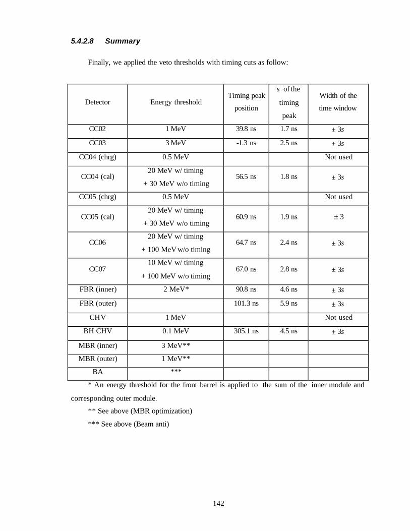
142

5.4.2.8 Summary

Finally, we applied the veto thresholds with timing cuts as follow:

Detector Energy threshold Timing peak

position

σ of the

timing

peak

Width of the

time window

CC02 1 MeV 39.8 ns 1.7 ns ± 3σ

CC03 3 MeV -1.3 ns 2.5 ns ± 3σ

CC04 (chrg) 0.5 MeV Not used

CC04 (cal) 20 MeV w/ timing

+ 30 MeV w/o timing 56.5 ns 1.8 ns ± 3σ

CC05 (chrg) 0.5 MeV Not used

CC05 (cal) 20 MeV w/ timing

+ 30 MeV w/o timing 60.9 ns 1.9 ns ± 3

CC06 20 MeV w/ timing

+ 100 MeV w/o timing 64.7 ns 2.4 ns ± 3σ

CC07 10 MeV w/ timing

+ 100 MeV w/o timing 67.0 ns 2.8 ns ± 3σ

FBR (inner) 2 MeV* 90.8 ns 4.6 ns ± 3σ

FBR (outer) 101.3 ns 5.9 ns ± 3σ

CHV 1 MeV Not used

BH CHV 0.1 MeV 305.1 ns 4.5 ns ± 3σ

MBR (inner) 3 MeV**

MBR (outer) 1 MeV**

BA ***

* An energy threshold for the front barrel is applied to the sum of the inner module and

corresponding outer module.

** See above (MBR optimization)

*** See above (Beam anti)

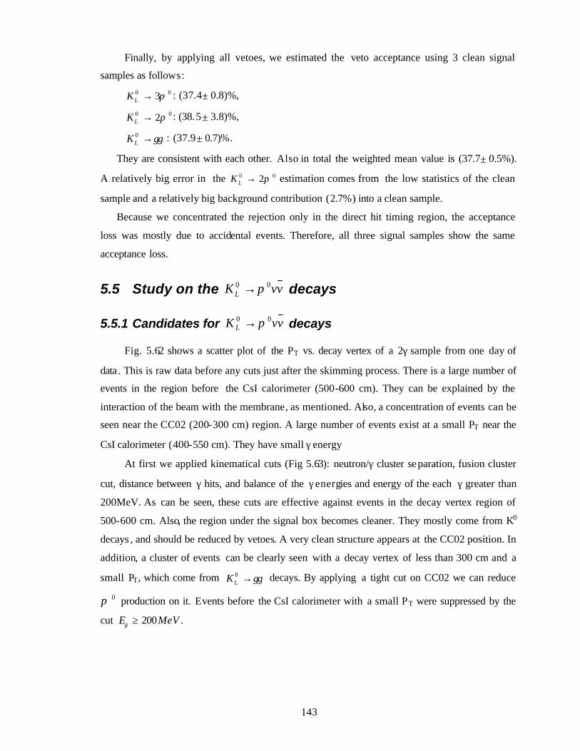
143

Finally, by applying all vetoes, we estimated the veto acceptance using 3 clean signal

samples as follows: 00 3π→LK : (37.4± 0.8)%,

00 2π→LK : (38.5± 3.8)%,

γγ→0LK : (37.9± 0.7)%.

They are consistent with each other. Also in total the weighted mean value is (37.7± 0.5%).

A relatively big error in the 00 2π→LK estimation comes from the low statistics of the clean

sample and a relatively big background contribution (2.7%) into a clean sample.

Because we concentrated the rejection only in the direct hit timing region, the acceptance

loss was mostly due to accidental events. Therefore, all three signal samples show the same

acceptance loss.

5.5 Study on the vvK L00 π→ decays

5.5.1 Candidates for vvK L

00 π→ decays

Fig. 5.62 shows a scatter plot of the PT vs. decay vertex of a 2γ sample from one day of

data . This is raw data before any cuts just after the skimming process. There is a large number of

events in the region before the CsI calorimeter (500-600 cm). They can be explained by the

interaction of the beam with the membrane, as mentioned. Also, a concentration of events can be

seen near the CC02 (200-300 cm) region. A large number of events exist at a small PT near the

CsI calorimeter (400-550 cm). They have small γ energy

At first we applied kinematical cuts (Fig 5.63): neutron/γ cluster separation, fusion cluster

cut, distance between γ hits, and balance of the γ energies and energy of the each γ greater than

200MeV. As can be seen, these cuts are effective against events in the decay vertex region of

500-600 cm. Also, the region under the signal box becomes cleaner. They mostly come from K0

decays , and should be reduced by vetoes. A very clean structure appears at the CC02 position. In

addition, a cluster of events can be clearly seen with a decay vertex of less than 300 cm and a

small PT, which come from γγ→0LK decays. By applying a tight cut on CC02 we can reduce

0π production on it. Events before the CsI calorimeter with a small PT were suppressed by the

cut MeVE 200≥γ .

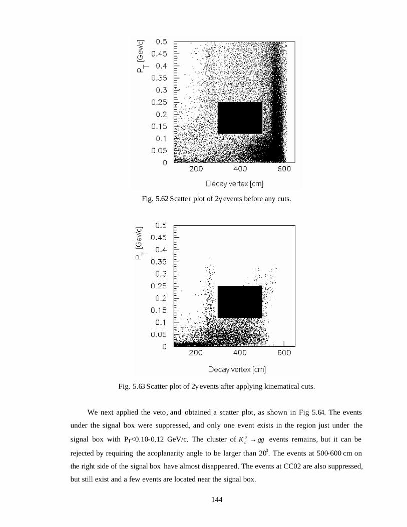
144

Fig. 5.62 Scatte r plot of 2γ events before any cuts.

Fig. 5.63 Scatter plot of 2γ events after applying kinematical cuts.

We next applied the veto, and obtained a scatter plot, as shown in Fig 5.64. The events

under the signal box were suppressed, and only one event exists in the region just under the

signal box with PT<0.10-0.12 GeV/c. The cluster of γγ→0LK events remains, but it can be

rejected by requiring the acoplanarity angle to be larger than 200. The events at 500-600 cm on

the right side of the signal box have almost disappeared. The events at CC02 are also suppressed,

but still exist and a few events are located near the signal box.

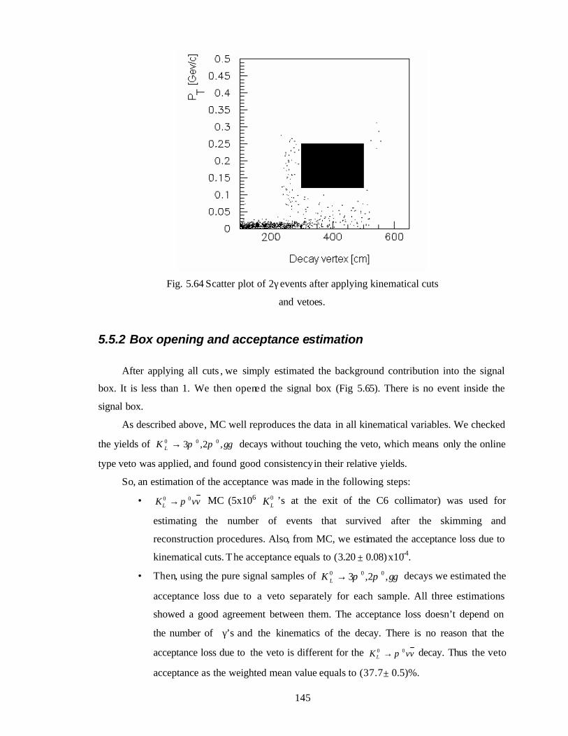
145

Fig. 5.64 Scatter plot of 2γ events after applying kinematical cuts

and vetoes.

5.5.2 Box opening and acceptance estimation

After applying all cuts , we simply estimated the background contribution into the signal

box. It is less than 1. We then opened the signal box (Fig 5.65). There is no event inside the

signal box.

As described above, MC well reproduces the data in all kinematical variables. We checked

the yields of γγππ ,2,3 000 →LK decays without touching the veto, which means only the online

type veto was applied, and found good consistency in their relative yields.

So, an estimation of the acceptance was made in the following steps:

• vvKL00 π→ MC (5x106 0

LK ’s at the exit of the C6 collimator) was used for

estimating the number of events that survived after the skimming and

reconstruction procedures. Also, from MC, we estimated the acceptance loss due to

kinematical cuts. The acceptance equals to (3.20 ± 0.08)x10-4.

• Then, using the pure signal samples of γγππ ,2,3 000 →LK decays we estimated the

acceptance loss due to a veto separately for each sample. All three estimations

showed a good agreement between them. The acceptance loss doesn’t depend on

the number of γ’s and the kinematics of the decay. There is no reason that the

acceptance loss due to the veto is different for the vvKL00 π→ decay. Thus the veto

acceptance as the weighted mean value equals to (37.7± 0.5)%.

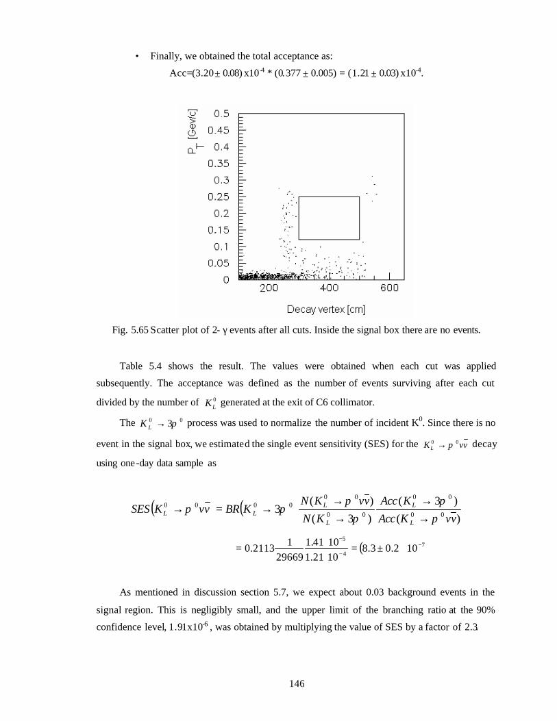
146

• Finally, we obtained the total acceptance as:

Acc=(3.20± 0.08) x10-4 * (0.377 ± 0.005) = (1.21 ± 0.03) x10-4.

Fig. 5.65 Scatter plot of 2- γ events after all cuts. Inside the signal box there are no events.

Table 5.4 shows the result. The values were obtained when each cut was applied

subsequently. The acceptance was defined as the number of events surviving after each cut

divided by the number of 0LK generated at the exit of C6 collimator.

The 00 3π→LK process was used to normalize the number of incident K0. Since there is no

event in the signal box, we estimated the single event sensitivity (SES) for the vvKL00 π→ decay

using one-day data sample as

( ) ( ))(

)3(

)3(

)(3 00

00

00

000000

vvKAcc

KAcc

KN

vvKNKBRvvKSES

L

L

L

LLL π

ππ

πππ

→→

→→

→=→

( ) 74

5

102.03.81021.11041.1

2966912113.0 −

−

−

⋅±=⋅⋅=

As mentioned in discussion section 5.7, we expect about 0.03 background events in the

signal region. This is negligibly small, and the upper limit of the branching ratio at the 90%

confidence level, 1.91x10-6 , was obtained by multiplying the value of SES by a factor of 2.3.

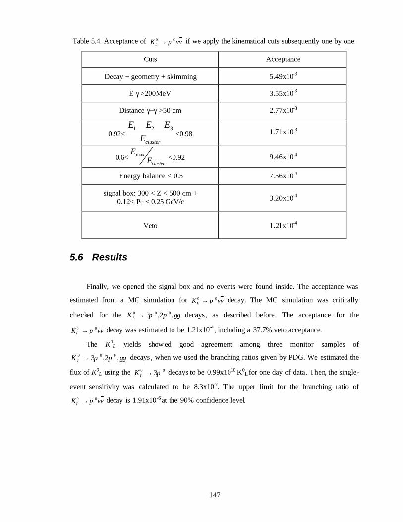
147

Table 5.4. Acceptance of vvKL00 π→ if we apply the kinematical cuts subsequently one by one.

Cuts Acceptance

Decay + geometry + skimming 5.49x10-3

E γ >200MeV 3.55x10-3

Distance γ−γ >50 cm 2.77x10-3

0.92<clusterE

EEE 321 ++<0.98 1.71x10-3

0.6<clusterE

Emax <0.92 9.46x10-4

Energy balance < 0.5 7.56x10-4

signal box: 300 < Z < 500 cm + 0.12< PT < 0.25 GeV/c 3.20x10-4

Veto 1.21x10-4

5.6 Results

Finally, we opened the signal box and no events were found inside. The acceptance was

estimated from a MC simulation for vvKL00 π→ decay. The MC simulation was critically

checked for the γγππ ,2,3 000 →LK decays, as described before. The acceptance for the

vvKL00 π→ decay was estimated to be 1.21x10-4, including a 37.7% veto acceptance.

The K0L yields show ed good agreement among three monitor samples of

γγππ ,2,3 000 →LK decays , when we used the branching ratios given by PDG. We estimated the

flux of K0L using the 00 3π→LK decays to be 0.99x1010 K0

L for one day of data. Then, the single-

event sensitivity was calculated to be 8.3x10-7. The upper limit for the branching ratio of

vvKL00 π→ decay is 1.91x10-6 at the 90% confidence level.

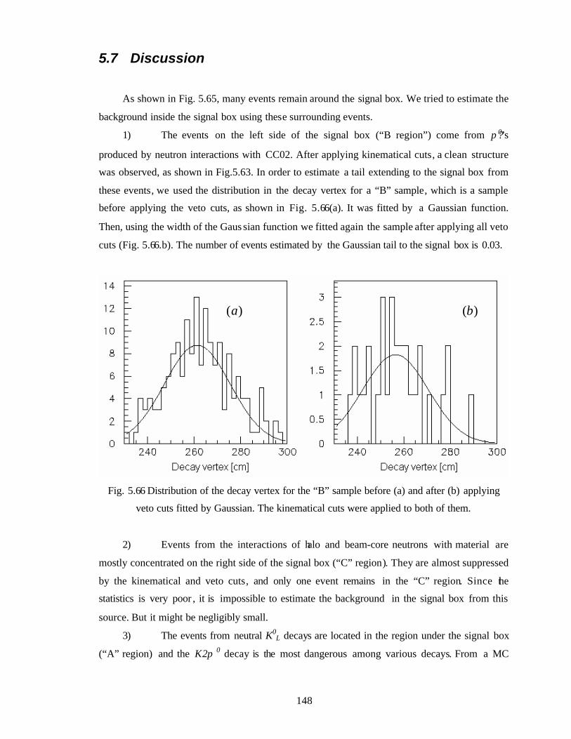
148

5.7 Discussion

As shown in Fig. 5.65, many events remain around the signal box. We tried to estimate the

background inside the signal box using these surrounding events.

1) The events on the left side of the signal box (“B region”) come from π?0’s

produced by neutron interactions with CC02. After applying kinematical cuts, a clean structure

was observed, as shown in Fig.5.63. In order to estimate a tail extending to the signal box from

these events, we used the distribution in the decay vertex for a “B” sample, which is a sample

before applying the veto cuts, as shown in Fig. 5.66(a). It was fitted by a Gaussian function.

Then, using the width of the Gaus sian function we fitted again the sample after applying all veto

cuts (Fig. 5.66.b). The number of events estimated by the Gaussian tail to the signal box is 0.03.

Fig. 5.66 Distribution of the decay vertex for the “B” sample before (a) and after (b) applying

veto cuts fitted by Gaussian. The kinematical cuts were applied to both of them.

2) Events from the interactions of halo and beam-core neutrons with material are

mostly concentrated on the right side of the signal box (“C” region). They are almost suppressed

by the kinematical and veto cuts, and only one event remains in the “C” region. Since the

statistics is very poor , it is impossible to estimate the background in the signal box from this

source. But it might be negligibly small.

3) The events from neutral K0L decays are located in the region under the signal box

(“A” region) and the K2π 0 decay is the most dangerous among various decays. From a MC

)(a )(b

149

sample of 10 day-statistics, no event was found in the signal box after applying all kinematical

and ve to cuts. So the background might be less than 0.1 event for one-day statistics.

The finite value of 0.03 events is only expected from item 1), which comes from π 0‘s

produced by halo neutrons at the CC02 position. It contains a margin to increase the statistics by

a factor of 33, which is comparable with our factor of 60 (full data/one-day data). The

improvement of the resolution might shrink the distribution of the decay vertex near CC02, and

also a decrease of the energy threshold of CC02 will improve the rejection of these events.

Other backgrounds are hard to estimate due to the low statistics of the data and MC ,

although their contribution might be small. A detailed study will be done in future analysis using

larger samples of one week and 1/3 data sets.

Since the single -event sensitivity for a one -day sample is 8.3x10-7, we will reach the level

of 1.8x10-8 in full statistics, if we simply extrapolate. It is poorer than the expected sensitivity of

3x10-10 by a factor of 60. One of the reasons is a small acceptance. Since the present acceptance

value of 1.21x10-4 includes the decay probability, we extracted the acceptance normalized for the

decays in our fiducial region (300-500cm). It is 0.6% and is smaller than the expected acceptance

of 8% by a factor of 13.

There are several points giving a remarkable acceptance loss, and can possibly be improve d.

At first, in the reconstruction procedure, we rejected events if the hit point of γ was outside of the

80 cm radius. It is related with poor reconstruction of the energy and hit position of a γ near the

border due to shower leakage from the CsI calorimeter which has a radius of about 100cm. By

increasing the reconstruction area up to 90 cm, we can improve the acceptance. More careful

treatment of the γ hits near and in KTeV crystals is also expected to increase the acceptance of

vvKL00 π→ .

Another point for a recovery of the acceptance exists in the cluster shape cuts. The

variables clusterE

Emax and clusterE

EEE 321 ++ were introduced to reject the neutron interaction and cluster

fusing in the CsI calorimeter. They are based on a simple estimation of the shower size, which

seems to be too simple. A detailed analysis of the difference in the shower shape for neutrons

and γ’s might be effective for neutron/ γ cluster separation, which allows us to save the

acceptance. Identification of the fused clusters can be also done based on the shower shape

analysis

As described in the section of background identification, we faced to the unexpected

background from the beam neutron interaction with a membrane. It produced a large peak in the

decay vertex distribution near the CsI calorimeter. At present , we had to introduce a tight cut for

150

the distance between γ hits. This also resulted in reducing the downstream end of the fiducial

volume (signal box) from 550cm (proposal) to 500cm. In this thesis we didn’t make the

optimization of the position of the signal box, which is potentially one of the sources to increase

the acceptance.

It is necessary to mention the veto study. To estimate the acceptance loss due to the veto

we used pure signal samples of the γγππ ,2,3 000 →LK decays. They show a good consistency

between all samples. The acceptance loss doesn’t depend on the number of γ’s and the

kinematics of the decay. This means that the acceptance loss does not come from backsplash, but

from accidental effects. In the present analysis we introduced rather sophisticated time windows

for the veto to understand it using the pure samples.

MBR is one of the most important veto detectors, which makes the biggest contribution to

the acceptance loss. We found that MBR is sensitive to a neutron passing through the modules ,

and a careful treatment of the time windows for the veto allows us to suppress the neutron events.

A more detailed study of veto might help to increase the acceptance.

Another reason of the poor sensitivity is a shorter beam time. Some part of the beam time

was lost due to problems related to the accelerator. Also, we spent some time f or the beam tuning

and detector calibration. In total, we collected about 60 days of data instead of the expected 100

days. After all, a factor of 3 remains as a decrease from the proposed value. It might come from

many sources, such as a difference of the KL spectrum from calculation, the dead time and the

target efficiency to produce K L.

In summary, we still have a possibility to recover the acceptance for the vvKL00 π→ decay

to reach the 10-9 -10-10 level of the single-event sensitivity. In any case it is important to reach

our goal of 3x10-10, because in the recent study of Buras [36] it is pointed out the branching ratio

of vvKL00 π→ might increase up to 3x10-10.

151

Chapter 6

Conclusion

The E391 experiment was successfully run for data taking from February 15 to June 1,

2004. All systems worked stably and no dead channels appeared during all period. The full

collected statistics of physics data is equivalent to 60 days of continuous data taken.

The E391 experiment is a pilot experiment, and it is important to check new techniques

used for searching for vvKL00 π→ decay. We confirmed most of them through an analysis of the

one-day data sample. The pencil beam clearly separates the γγ→0LK decays from other decay

modes using PT. The separation of the vacuum volumes into two regions by a thin membrane

allowed us to evacuate the air efficiently. The vacuum level could reach 10-4 Pa after 1 day of

evacuation. We could apply a very low veto threshold of a few MeV to the veto detectors.

In the present first step of analysis using one day of data, we could develop various

software tools and confirm the good quality of data.

• We could establish in-situ calibration of detectors. All detectors were

calibrated using punch-though or cosmic muons. For the CsI calorimeter we

152

refined the calibration by using γ’s from π 0 decays produced on a target. Also,

all detectors showed good stability.

• We developed GEANT-3 MC simulation and reconstruction codes. The

reconstruction code was applied to both data and MC. MC well reproduces the

experimental spectra of various kinematical variables. We developed one of

the analysis methods using pure signal samples of the K3π 0 (~30k events),

K2π 0 (~1k events) and Kγγ (~13k events) decays. The purification process

relayed a negligibly small contamination of for K3π 0, 2.7% for K2π 0 and

0.7% for Kγγ. We prepared background samples of the K2π 0 and Kγγ decays.

The pure signal samples showed a good agreement between the data and the

MC. The relative branching ratios obtained from three pure samples are in a

good agreement with those given by PDG.

• Background sources were explored by comparing the data with the MC at the

level of online for 2-γ events. They are the decays of K3π 0, K2π 0, Kγγ, and

K –>π 0π +π -, ha lo neutron interaction with CC02 and CHV. However, we

found additional background sources: two clusters due to a hadronic shower in

the CsI calorimeter produced by a single neutron and interactions of the beam

core neutrons with the membrane. We then developed several kinematical and

cluster shape cuts to suppress the background due to the neutron interaction.

• The acceptance loss due to the veto was surely estimated from pure signal

samples. Since we found a severe effect of backsplash, we developed a time

window for the veto signal.

Finally, we obtained the upper limit for the branching ratio of vvKL00 π→ decay to be

1.91x10-6 (90% CL).

In summary, the present analysis using a one-day sample was very valuable to check

several techniques newly developed for the vvKL00 π→ measurement. It was also very important

to understand the data quality and to find unexpected phenomena. Not only the methods

developed in the present analysis are being applied for the analysis of a larger sample, but also

the results are reflected to several upgrades of the detector system for the second run, which was

just started in the middle of January 2005.

153

References

1. H. Christenson et al. Phys. Rev. Lett. 13, 138 (1964)

2. K.Abe et.al. Phys. Rev. Lett 87, 091802 (2001).

3. T. Inagaki et al., “Measurement of the vvK L00 π→ decay”, KEK Internal

96-13 (1996)

4. A.J. Buras, hep-ph/9905437 (1999)

5. M. Koboyahsi and T. Msakawa, Prog. Theor. Phys. 49, 652 (1973)

6. L. Wolfenstein. Phys. Rev. Let. 51, 1945 (1983)

7. Phys. Lett. B592, 130 (2004)

8. I.S. Towner and J.C Hardy, nucl-th/9809087 (1998)

9. Yu.A.Mostovoi et al. Phys. Atomic Nucl. 64 (2001)

10. Phys. Lett. B592, 131 (2004)

11. V. Cirigliano et al. Eur. Phys. J. C23,121 (2002)

12. P.Abreu et al. Phys. Lett. B439 ,209 (1998)

13. The LEP Collaborations et al. hep-exp/0112021 (2002)

14. Phys. Lett. B592, 134 (2004)

15. Phys. Lett. B592, 133 (2004)

16. hep-ph/0304132 (2003)

17. Phys. Lett. B592, 131 (2004)

18. Phys. Lett. B592, 793 (2004)

19. T.Affolder. Phys. Rev. Lett. 86, 3233 (2001)

20. Phys. Lett. B592, 140 (2004)

21. Phys Rev.Lett.89,211802 (2002)

22. R. Belusevic “Neutral kaon”, KEK preprint 97-264 (1998)

23. T Inami and C.S. Lim, Prog, Theor, Phys. 65, 297 (1981)

24. W Marciano and Z Parsa, Phys. Rev.D53, R1 (1996)

25. G Buchalla et al., Rev Mod. Phys 68, 1125 (1989)

26. G. Buchalla, hep-ph/9612307 (1996).

154

27. S. Plaszczynski and M.H Schune, hep-ph/9911280 (1999).

28. L. Silvestrini et al., hep-ph/0009248 (2000).

29. A. Buras et al., hep-ph/0007313 (2000).

30. M. Brhlik, hep-ph/990948 (1999).

31. M.S. Canowitz, hep-ph/9905478 (1999).

32. T. Hattori et al., hep-ph/9908447 (1999).

33. Z. Xiao et al., hep-ph/9903348 (1999).

34. Z. Xiao et al., hep-ph/9903347 (1999).

35. Y. Kiyo et al., hep-ph/9900948 (1998).

36. A.Buras hep-ph/0312259 (2004)

37. K.Abe et al. hep-ex/0308040 (2003)

38. B.Aubert et al. hep-ex/0308012 (2003)

39. A.Alavi-Harati et al. Phys.Rev. D61, 072006 (2000)

40. J.Adams et al. hep-ex/9806007 (1998)

41. KEK Preprint 2004-85 H (Will be published in NIM)

42. Particle Data Group, Phys.Lett. B592, (2004)

43. KEK Preprint 2004-86 H (Will be published in NIM)