A matricial Hilbert transform on closed surfaces in ... › ... › Main › deknock.pdf ·...
40
Introduction The HT on ∂Γ in Euclidean CA Hermitean CA A matricial HT on ∂Γ in Hermitean CA References A matricial Hilbert transform on closed surfaces in Hermitean Clifford analysis Fred Brackx Bram De Knock Hennie De Schepper Clifford Research Group, Ghent University, Belgium AGACSE 2008, Grimma August 17–19, 2008 Bram De Knock A matricial HT on closed surfaces in Hermitean CA
Transcript of A matricial Hilbert transform on closed surfaces in ... › ... › Main › deknock.pdf ·...

Introduction The HT on ∂Γ in Euclidean CA Hermitean CA A matricial HT on ∂Γ in Hermitean CA References
A matricial Hilbert transformon closed surfaces
in Hermitean Clifford analysis
Fred Brackx Bram De Knock Hennie De Schepper
Clifford Research Group, Ghent University, Belgium
AGACSE 2008, GrimmaAugust 17–19, 2008
Bram De Knock A matricial HT on closed surfaces in Hermitean CA
Introduction The HT on ∂Γ in Euclidean CA Hermitean CA A matricial HT on ∂Γ in Hermitean CA References
Outline
1 Introduction: the Hilbert transform on the real line
2 The Hilbert transform on closed surfaces in Euclidean Cliffordanalysis
3 Hermitean Clifford analysis
4 A matricial Hilbert transform on closed surfaces in HermiteanClifford analysis
Bram De Knock A matricial HT on closed surfaces in Hermitean CA
Introduction The HT on ∂Γ in Euclidean CA Hermitean CA A matricial HT on ∂Γ in Hermitean CA References
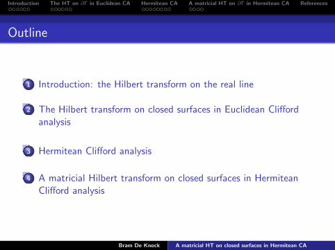
definition (Hilbert)
consider finite energy signals f , i.e. f ∈ L2(R), so
‖f ‖2L2(R) =
∫ +∞
−∞|f (t)|2 dt < +∞
then, the Hilbert transform H[f] of f
H[f ](t) =1
πPv
∫ +∞
−∞
f (x)
t − xdx
=1
πlimε→0+
∫|t−x |>ε
f (x)
t − xdx
= (H ∗ f ) (t)
with the Hilbert kernel H
H(x) = Pv1
πx
Bram De Knock A matricial HT on closed surfaces in Hermitean CA

Introduction The HT on ∂Γ in Euclidean CA Hermitean CA A matricial HT on ∂Γ in Hermitean CA References
properties (Hardy & Titchmarsh)
1 the Hilbert operator H is translation invariant, i.e.
τa[H[f ]] = H[τa[f ]] , with τa[f ](t) = f (t − a) , a ∈ R
2 the Hilbert operator H is dilation invariant, i.e.
da[H[f ]] = H[da[f ]] , with da[f ](t) =1√a
f (t
a) , a > 0
3 the Hilbert operator H is a bounded linear operator onL2(R), and is a fortiori norm preserving, i.e.
‖H[f ]‖L2(R) = ‖f ‖L2(R)
Bram De Knock A matricial HT on closed surfaces in Hermitean CA

Introduction The HT on ∂Γ in Euclidean CA Hermitean CA A matricial HT on ∂Γ in Hermitean CA References
properties (Hardy & Titchmarsh)
4 H2 = −1 on L2(R), and hence H−1 = −H
5 the Hilbert operator H is unitary on L2(R), i.e.
HH∗ = H∗H = 1
with its adjoint H∗ given by −H, i.e.
(H[f ], g)L2(R) = (f ,−H[g ])L2(R)
6 the Hilbert operator H commutes with differentiation, i.e.if f and f ′ are in L2(R), then
H[
d
dtf (t)
](x) =
d
dx[H[f ](x)]
Bram De Knock A matricial HT on closed surfaces in Hermitean CA
Introduction The HT on ∂Γ in Euclidean CA Hermitean CA A matricial HT on ∂Γ in Hermitean CA References
properties (Hardy & Titchmarsh)
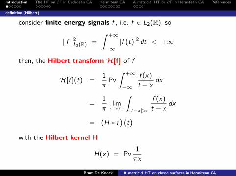
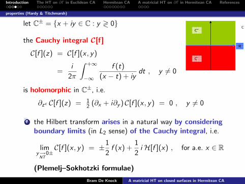
let C± = x + iy ∈ C : y ≷ 0
the Cauchy integral C[f]
C[f ](z) = C[f ](x , y)
=i
2π
∫ +∞
−∞
f (t)
(x − t) + iydt , y 6= 0
is holomorphic in C±, i.e.
∂zc C[f ](z) = 12 (∂x + i∂y ) C[f ](x , y) = 0 , y 6= 0
7 the Hilbert transform arises in a natural way by consideringboundary limits (in L2 sense) of the Cauchy integral, i.e.
limy→
NT0±C[f ](x , y) = ±1
2f (x) +
1
2i H[f ](x) , for a.e. x ∈ R
(Plemelj–Sokhotzki formulae)
Bram De Knock A matricial HT on closed surfaces in Hermitean CA
Introduction The HT on ∂Γ in Euclidean CA Hermitean CA A matricial HT on ∂Γ in Hermitean CA References
properties (Hardy & Titchmarsh)
let C± = x + iy ∈ C : y ≷ 0
the Cauchy integral C[f]
C[f ](z) = C[f ](x , y)
=i
2π
∫ +∞
−∞
f (t)
(x − t) + iydt , y 6= 0
is holomorphic in C±, i.e.
∂zc C[f ](z) = 12 (∂x + i∂y ) C[f ](x , y) = 0 , y 6= 0
7 the Hilbert transform arises in a natural way by consideringboundary limits (in L2 sense) of the Cauchy integral, i.e.
limy→
NT0±C[f ](x , y) = ±1
2f (x) +
1
2i H[f ](x) , for a.e. x ∈ R
(Plemelj–Sokhotzki formulae)
Bram De Knock A matricial HT on closed surfaces in Hermitean CA
Introduction The HT on ∂Γ in Euclidean CA Hermitean CA A matricial HT on ∂Γ in Hermitean CA References
some applications
signal processing
metallurgy (theory of elasticity)
Dirichlet boundary value problems (potential theory)
dispersion relation in high energy physics, spectroscopy andwave equations
wing theory
harmonic analysis
notice: applications were not discussed in my research
Bram De Knock A matricial HT on closed surfaces in Hermitean CA
Introduction The HT on ∂Γ in Euclidean CA Hermitean CA A matricial HT on ∂Γ in Hermitean CA References
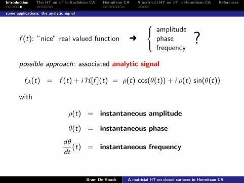
some applications: the analytic signal
f (t): ”nice” real valued function Ü
amplitude
?phasefrequency
possible approach: associated analytic signal
fA(t) = f (t) + i H[f ](t)
= ρ(t) cos(θ(t)) + i ρ(t) sin(θ(t))
with
ρ(t) = instantaneous amplitude
θ(t) = instantaneous phase
dθ
dt(t) = instantaneous frequency
Bram De Knock A matricial HT on closed surfaces in Hermitean CA
Introduction The HT on ∂Γ in Euclidean CA Hermitean CA A matricial HT on ∂Γ in Hermitean CA References
some applications: the analytic signal
f (t): ”nice” real valued function Ü
amplitude
?phasefrequency
possible approach: associated analytic signal
fA(t) = f (t) + i H[f ](t) = ρ(t) cos(θ(t)) + i ρ(t) sin(θ(t))
with
ρ(t) = instantaneous amplitude
θ(t) = instantaneous phase
dθ
dt(t) = instantaneous frequency
Bram De Knock A matricial HT on closed surfaces in Hermitean CA

Introduction The HT on ∂Γ in Euclidean CA Hermitean CA A matricial HT on ∂Γ in Hermitean CA References
Outline
1 Introduction: the Hilbert transform on the real line
2 The Hilbert transform on closed surfaces in Euclidean Cliffordanalysis
3 Hermitean Clifford analysis
4 A matricial Hilbert transform on closed surfaces in HermiteanClifford analysis
Bram De Knock A matricial HT on closed surfaces in Hermitean CA

Introduction The HT on ∂Γ in Euclidean CA Hermitean CA A matricial HT on ∂Γ in Hermitean CA References
why study higher dimensional Hilbert transforms?
1D signal processing:
1D Hilbert transform is used to construct analytic signal inorder to extract interesting features (amplitude, phase,frequency) of real 1D signal
mD signal processing (e.g. images (2D), video signals (3D)):
mD Hilbert transform as a tool to obtain interesting mDsignal information
Bram De Knock A matricial HT on closed surfaces in Hermitean CA

Introduction The HT on ∂Γ in Euclidean CA Hermitean CA A matricial HT on ∂Γ in Hermitean CA References
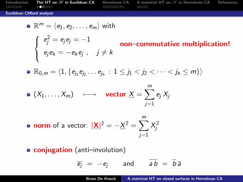
Euclidean Clifford analysis
Rm = 〈e1, e2, . . . , em〉 withe2j = ejej = −1
non–commutative multiplication!ejek = −ekej , j 6= k
R0,m = 〈1, ej1ej2 . . . ejh : 1 ≤ j1 < j2 < · · · < jh ≤ m〉
(X1, . . . ,Xm) ←→ vector X =m∑
j=1
ej Xj
norm of a vector: |X|2 = −X 2 =m∑
j=1
X 2j
conjugation (anti–involution)
ej = −ej and a b = b a
Bram De Knock A matricial HT on closed surfaces in Hermitean CA
Introduction The HT on ∂Γ in Euclidean CA Hermitean CA A matricial HT on ∂Γ in Hermitean CA References
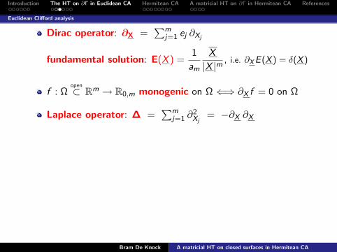
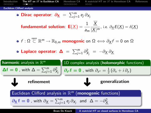
Euclidean Clifford analysis
Dirac operator: ∂X =∑m
j=1 ej ∂Xj
fundamental solution: E(X ) =1
am
X
|X |m, i.e. ∂X E (X ) = δ(X )
f : Ωopen
⊂ Rm → R0,m monogenic on Ω ⇐⇒ ∂X f = 0 on Ω
Laplace operator: ∆ =∑m
j=1 ∂2Xj
= −∂X ∂X
harmonic analysis in Rm
∆f = 0 , with ∆ =∑m
j=1 ∂2XjÜ
refinement
1D complex analysis (holomorphic functions)
∂zcf = 0 , with ∂zc = 12 (∂x + i ∂y )
Ü
generalization
Euclidean Clifford analysis in Rm (monogenic functions)
∂X f = 0 , with ∂X =∑m
j=1 ej ∂Xjand ∆ = −∂2
X
Bram De Knock A matricial HT on closed surfaces in Hermitean CA
Introduction The HT on ∂Γ in Euclidean CA Hermitean CA A matricial HT on ∂Γ in Hermitean CA References
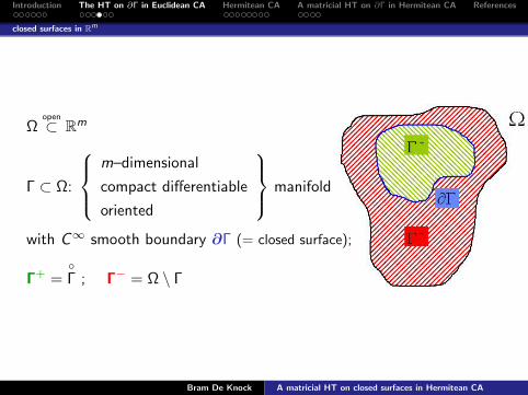
closed surfaces in Rm
Ωopen
⊂ Rm
Γ ⊂ Ω:
m–dimensional
compact differentiable
oriented
manifold
with C∞ smooth boundary ∂Γ (= closed surface);
Γ+ =Γ ; Γ− = Ω \ Γ
Bram De Knock A matricial HT on closed surfaces in Hermitean CA
Introduction The HT on ∂Γ in Euclidean CA Hermitean CA A matricial HT on ∂Γ in Hermitean CA References
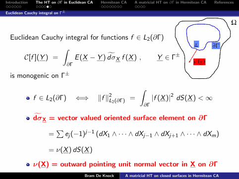
Euclidean Cauchy integral on Γ±
Euclidean Cauchy integral for functions f ∈ L2(∂Γ)
C[f ](Y ) =
∫∂Γ
E (X − Y ) dσX f (X ) , Y ∈ Γ±
is monogenic on Γ±
f ∈ L2(∂Γ) ⇐⇒ ‖f ‖2L2(∂Γ) =
∫∂Γ|f (X )|2 dS(X ) <∞
dσX = vector valued oriented surface element on ∂Γ
=∑
ej(−1)j−1 (dX1 ∧ · · · ∧ dXj−1 ∧ dXj+1 ∧ · · · ∧ dXm)
= ν(X ) dS(X )
ν(X) = outward pointing unit normal vector in X on ∂Γ
Bram De Knock A matricial HT on closed surfaces in Hermitean CA
Introduction The HT on ∂Γ in Euclidean CA Hermitean CA A matricial HT on ∂Γ in Hermitean CA References
Euclidean Hilbert transform on ∂Γ
definition
the Euclidean Hilbert transform arises in a natural way byconsidering boundary limits (in L2 sense) of the Euclidean Cauchyintegral, i.e.
limY→UY∈Γ±
C[f ](Y ) = ±1
2f (U) +
1
2H[f ](U) , U ∈ ∂Γ
with the Euclidean Hilbert transform
H[f ](U) = 2 Pv
∫∂Γ
E (X − U) dσX f (X ) , U ∈ ∂Γ
properties
1 H is a bounded linear operator on L2(∂Γ)
2 H2 = 1 on L2(∂Γ)
3 H∗ = νH ν on L2(∂Γ), i.e. 〈H[f ], g〉 = 〈f , νH[νg ]〉Bram De Knock A matricial HT on closed surfaces in Hermitean CA
Introduction The HT on ∂Γ in Euclidean CA Hermitean CA A matricial HT on ∂Γ in Hermitean CA References
Outline
1 Introduction: the Hilbert transform on the real line
2 The Hilbert transform on closed surfaces in Euclidean Cliffordanalysis
3 Hermitean Clifford analysis
4 A matricial Hilbert transform on closed surfaces in HermiteanClifford analysis
Bram De Knock A matricial HT on closed surfaces in Hermitean CA
Introduction The HT on ∂Γ in Euclidean CA Hermitean CA A matricial HT on ∂Γ in Hermitean CA References
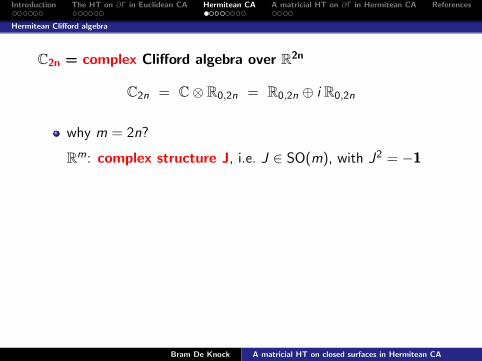
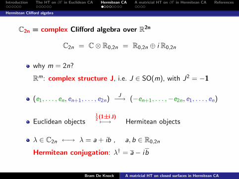
Hermitean Clifford algebra
C2n = complex Clifford algebra over R2n
C2n = C⊗ R0,2n = R0,2n ⊕ i R0,2n
why m = 2n?
Rm: complex structure J, i.e. J ∈ SO(m), with J2 = −1
(e1, . . . , en, en+1, . . . , e2n)J−→ (−en+1, . . . ,−e2n, e1, . . . , en)
Euclidean objects12
(1±i J)7−→ Hermitean objects
λ ∈ C2n ←→ λ = a + ib , a, b ∈ R0,2n
Hermitean conjugation: λ† = a− ib
Bram De Knock A matricial HT on closed surfaces in Hermitean CA
Introduction The HT on ∂Γ in Euclidean CA Hermitean CA A matricial HT on ∂Γ in Hermitean CA References
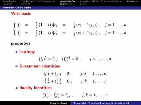
Hermitean Clifford algebra
Witt basis
fj = 1
2 (1 + iJ)[ej ] = 12 (ej − i en+j) , j = 1, . . . , n
f†j = −1
2 (1− iJ)[ej ] = −12 (ej + i en+j) , j = 1, . . . , n
properties
isotropy
(fj)2 = 0 , (f†j )2 = 0 , j = 1, . . . , n
Grassmann identities
fj fk + fk fj = 0 , j , k = 1, . . . , n
f†j f†k + f
†k f†j = 0 , j , k = 1, . . . , n
duality identities
fj f†k + f
†k fj = δjk , j , k = 1, . . . , n
Bram De Knock A matricial HT on closed surfaces in Hermitean CA
Introduction The HT on ∂Γ in Euclidean CA Hermitean CA A matricial HT on ∂Γ in Hermitean CA References
Hermitean Clifford algebra
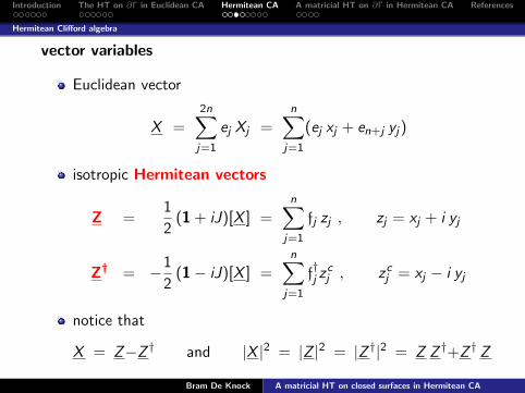
vector variables
Euclidean vector
X =2n∑j=1
ej Xj =n∑
j=1
(ej xj + en+j yj)
isotropic Hermitean vectors
Z =1
2(1 + iJ)[X ] =
n∑j=1
fj zj , zj = xj + i yj
Z† = −1
2(1− iJ)[X ] =
n∑j=1
f†j zc
j , zcj = xj − i yj
notice that
X = Z−Z † and |X |2 = |Z |2 = |Z †|2 = Z Z †+Z † Z
Bram De Knock A matricial HT on closed surfaces in Hermitean CA

Introduction The HT on ∂Γ in Euclidean CA Hermitean CA A matricial HT on ∂Γ in Hermitean CA References
Hermitean Clifford algebra
Dirac operators
Euclidean Dirac operator
∂X =2n∑j=1
ej ∂Xj=
n∑j=1
(ej ∂xj + en+j ∂yj )
isotropic Hermitean Dirac operators
∂Z† =1
4(1 + iJ)[∂X ] =
n∑j=1
fj ∂zcj, ∂zc
j=
1
2
(∂xj + i ∂yj
)∂Z = −1
4(1− iJ)[∂X ] =
n∑j=1
f†j ∂zj , ∂zj =
1
2
(∂xj − i ∂yj
)notice that
∂X = 2(∂Z† − ∂Z
)and ∆ = 4
(∂Z∂Z† + ∂Z†∂Z
)g : Ω→ C2n is (Hermitean or) h–monogenic if and only if
∂Z g = 0 and ∂Z†g = 0Bram De Knock A matricial HT on closed surfaces in Hermitean CA
Introduction The HT on ∂Γ in Euclidean CA Hermitean CA A matricial HT on ∂Γ in Hermitean CA References
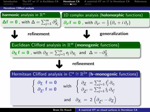
Hermitean Clifford analysis
harmonic analysis in Rm
∆f = 0 , with ∆ =∑m
j=1 ∂2XjÜ
refinement
1D complex analysis (holomorphic functions)
∂zcf = 0 , with ∂zc = 12 (∂x + i ∂y )
Ü
generalization
Euclidean Clifford analysis in Rm (monogenic functions)
∂X f = 0 , with ∂X =∑m
j=1 ej ∂Xjand ∆ = −∂2
XÜ
refinement
Hermitean Clifford analysis in Cn ∼= R2n (h–monogenic functions)∂Z f = 0
∂Z† f = 0with
∂Z =
∑nj=1 f
†j ∂zj
∂Z† =∑n
j=1 fj ∂zcj
and ∂X = 2(∂Z† − ∂Z
)Bram De Knock A matricial HT on closed surfaces in Hermitean CA

Introduction The HT on ∂Γ in Euclidean CA Hermitean CA A matricial HT on ∂Γ in Hermitean CA References
Hermitean Clifford analysis
further development: need for a Cauchy integral formula forh–monogenic functions
put:
E(Z ,Z †) = −(1 + i J)[E (X )]
E†(Z ,Z †) = (1− i J)[E (X )]
introducing the particular circulant (2× 2) matrices
D(Z ,Z†) =
(∂Z ∂Z†
∂Z† ∂Z
), E =
(E E†E† E
), δ =
(δ 00 δ
)one obtains that
D(Z,Z†) E(Z ,Z †) = δ(Z )
Bram De Knock A matricial HT on closed surfaces in Hermitean CA
Introduction The HT on ∂Γ in Euclidean CA Hermitean CA A matricial HT on ∂Γ in Hermitean CA References
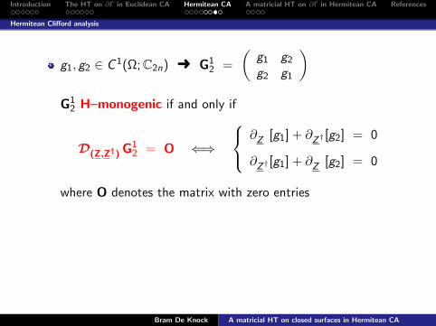
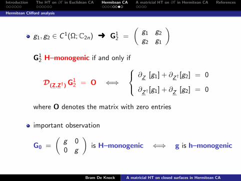
Hermitean Clifford analysis
g1, g2 ∈ C 1(Ω; C2n) Ü G12 =
(g1 g2
g2 g1
)G1
2 H–monogenic if and only if
D(Z,Z†) G12 = O ⇐⇒
∂Z [g1] + ∂Z† [g2] = 0
∂Z† [g1] + ∂Z [g2] = 0
where O denotes the matrix with zero entries
important observation
G0 =
(g 00 g
)is H–monogenic ⇐⇒ g is h–monogenic
Bram De Knock A matricial HT on closed surfaces in Hermitean CA
Introduction The HT on ∂Γ in Euclidean CA Hermitean CA A matricial HT on ∂Γ in Hermitean CA References
Hermitean Clifford analysis
g1, g2 ∈ C 1(Ω; C2n) Ü G12 =
(g1 g2
g2 g1
)G1
2 H–monogenic if and only if
D(Z,Z†) G12 = O ⇐⇒
∂Z [g1] + ∂Z† [g2] = 0
∂Z† [g1] + ∂Z [g2] = 0
where O denotes the matrix with zero entries
important observation
G0 =
(g 00 g
)is H–monogenic ⇐⇒ g is h–monogenic
Bram De Knock A matricial HT on closed surfaces in Hermitean CA

Introduction The HT on ∂Γ in Euclidean CA Hermitean CA A matricial HT on ∂Γ in Hermitean CA References
Hermitean Clifford analysis
volume element on Γ:
dW(Z,Z†) = (dz1 ∧ dzc1 ) ∧ (dz2 ∧ dzc
2 ) ∧ · · · ∧ (dzn ∧ dzcn )
matricial Hermitean oriented surface element on ∂Γ:
dΣ(Z,Z†) =
(dσZ −dσZ†
−dσZ† dσZ
)with
dσZ =n∑
j=1
f†j dzj , dσZ† =
n∑j=1
fj dzcj
and
dzj = (dz1 ∧ dzc1 ) ∧ · · · ∧ ([dzj ] ∧ dzc
j ) ∧ · · · ∧ (dzn ∧ dzcn )
dzcj = (dz1 ∧ dzc
1 ) ∧ · · · ∧ (dzj ∧ [dzcj ]) ∧ · · · ∧ (dzn ∧ dzc
n )
Bram De Knock A matricial HT on closed surfaces in Hermitean CA
Introduction The HT on ∂Γ in Euclidean CA Hermitean CA A matricial HT on ∂Γ in Hermitean CA References
Outline
1 Introduction: the Hilbert transform on the real line
2 The Hilbert transform on closed surfaces in Euclidean Cliffordanalysis
3 Hermitean Clifford analysis
4 A matricial Hilbert transform on closed surfaces in HermiteanClifford analysis
Bram De Knock A matricial HT on closed surfaces in Hermitean CA

Introduction The HT on ∂Γ in Euclidean CA Hermitean CA A matricial HT on ∂Γ in Hermitean CA References
three steps away from a Hermitean Cauchy integral
1 Clifford–Stokes theorems
Theorem (Euclidean Clifford–Stokes theorem)
Let f and g be functions in C 1(Ω; R0,2n), then∫∂Γ
f (X ) dσX g(X ) =
∫Γ
[(f ∂X ) g + f (∂X g)
]dV (X )
Theorem (Hermitean Clifford–Stokes theorem)
Let f1, f2, g1 and g2 be functions in C 1(Ω; C2n) and let F12 and G1
2
be their respective associated matrix functions, then∫∂Γ
F12(X ) dΣ(Z ,Z†) G1
2(X )
=
∫Γ
[(F1
2 D(Z ,Z†)) G12 + F1
2 (D(Z ,Z†) G12)]
dW (Z ,Z †)
Bram De Knock A matricial HT on closed surfaces in Hermitean CA

Introduction The HT on ∂Γ in Euclidean CA Hermitean CA A matricial HT on ∂Γ in Hermitean CA References
three steps away from a Hermitean Cauchy integral
2 Cauchy–Pompeiu formulae
Theorem (Euclidean Cauchy–Pompeiu formula)
Let g ∈ C 1(Ω; R0,2n), then∫∂Γ
E (X−Y )dσX g−∫
ΓE (X−Y )
(∂X g
)dV (X ) =
0 , Y ∈ Γ−
g(Y ) , Y ∈ Γ+
Theorem (Hermitean Cauchy–Pompeiu formula)
Let g1 and g2 be functions in C 1(Ω; C2n) and let G12 be the
associated matrix function, then∫∂ΓE(Z −V ) dΣ(Z ,Z†) G1
2−∫
ΓE(Z −V )
(D(Z ,Z†)G
12
)dW (Z ,Z †)
=
O , Y ∈ Γ−
(−1)n(n+1)
2 (2i)n G12(Y ) , Y ∈ Γ+
Bram De Knock A matricial HT on closed surfaces in Hermitean CA

Introduction The HT on ∂Γ in Euclidean CA Hermitean CA A matricial HT on ∂Γ in Hermitean CA References
three steps away from a Hermitean Cauchy integral
3 Cauchy integral formulae
Theorem (Euclidean Cauchy integral formula)
If the function g : Ω→ R0,2n is monogenic, then∫∂Γ
E (X − Y ) dσX g(X ) =
0 , Y ∈ Γ−
g(Y ) , Y ∈ Γ+
Theorem (Hermitean Cauchy integral formula I)
Let g1 and g2 be functions in C 1(Ω; C2n) and let G12 be the
associated matrix function. If G12 is H–monogenic, then∫
∂ΓE(Z−V ) dΣ(Z ,Z†) G1
2(X ) =
O , Y ∈ Γ−
(−1)n(n+1)
2 (2i)n G12(Y ) , Y ∈ Γ+
Theorem (Hermitean Cauchy integral formula II)
If the function g : Ω→ C2n is h–monogenic, then∫∂ΓE(Z−V ) dΣ(Z ,Z†) G0(X ) =
O , Y ∈ Γ−
(−1)n(n+1)
2 (2i)n G0(Y ) , Y ∈ Γ+
Bram De Knock A matricial HT on closed surfaces in Hermitean CA

Introduction The HT on ∂Γ in Euclidean CA Hermitean CA A matricial HT on ∂Γ in Hermitean CA References
three steps away from a Hermitean Cauchy integral
3 Cauchy integral formulae
Theorem (Euclidean Cauchy integral formula)
If the function g : Ω→ R0,2n is monogenic, then∫∂Γ
E (X − Y ) dσX g(X ) =
0 , Y ∈ Γ−
g(Y ) , Y ∈ Γ+
Theorem (Hermitean Cauchy integral formula II)
If the function g : Ω→ C2n is h–monogenic, then∫∂ΓE(Z−V ) dΣ(Z ,Z†) G0(X ) =
O , Y ∈ Γ−
(−1)n(n+1)
2 (2i)n G0(Y ) , Y ∈ Γ+
Bram De Knock A matricial HT on closed surfaces in Hermitean CA

Introduction The HT on ∂Γ in Euclidean CA Hermitean CA A matricial HT on ∂Γ in Hermitean CA References
a matricial Hilbert transform in Hermitean Clifford analysis
Hermitean Cauchy integral C
C[G12](Y ) =
∫∂ΓE(Z − V ) dΣ(Z ,Z†) G1
2(X ) , Y ∈ Γ±
for functions g1, g2 ∈ C 0(∂Γ)
Hermitean Hilbert transform Hdefinition
limY→UY∈Γ±
C[G12](Y ) = (−1)
n(n+1)2 (2i)n
(±1
2G1
2(U) +1
2H[G1
2](U)
), U ∈ ∂Γ
for functions g1, g2 ∈ L2(∂Γ)
properties1 H is a bounded linear operator on L2(∂Γ)
2 H2 = E2 on L2(∂Γ)
3 H∗ = VHV on L2(∂Γ)
Bram De Knock A matricial HT on closed surfaces in Hermitean CA
Introduction The HT on ∂Γ in Euclidean CA Hermitean CA A matricial HT on ∂Γ in Hermitean CA References
To read: Hermitean Clifford analysis
F. Brackx, H. De Schepper, F. Sommen,The Hermitean Clifford analysis toolbox,to appear in Adv. Appl. Clifford Alg.
F. Brackx, J. Bures, H. De Schepper, D. Eelbode, F. Sommen,V. Soucek,Fundaments of Hermitean Clifford Analysis. Part I: Complexstructure,Complex Anal. Oper. Theory 1(3) (2007), 341-365.
F. Brackx, J. Bures, H. De Schepper, D. Eelbode, F. SommenV. Soucek,Fundaments of Hermitean Clifford Analysis. Part II: Splittingof h-monogenic equations,Complex Var. Elliptic Equ. 52(1011) (2007), 1063-1079.
Bram De Knock A matricial HT on closed surfaces in Hermitean CA

Introduction The HT on ∂Γ in Euclidean CA Hermitean CA A matricial HT on ∂Γ in Hermitean CA References
To read: Hermitean Hilbert transform
F. Brackx, B. De Knock, H. De Schepper, D. Pena Pena, F.Sommen,On Cauchy and Martinelli–Bochner integral formulae inHermitean Clifford analysis,submitted.
F. Brackx, B. De Knock, H. De Schepper,A matrix Hilbert transform in Hermitean Clifford analysis,J. Math. Anal. Appl. 344(2) (2008), 1068-1078.
Bram De Knock A matricial HT on closed surfaces in Hermitean CA
![Ba^QdPc E RPW lPMcW^] - Farnell element145 P^\_McWOWZWch 5 § 5 @^ §@^ BVhbWPMZ EWjR HI g : g 5 I \\ ?MW] J J 7a^]c E_RMYRa J J 4R]cRa E_RMYRa J J DRMa E_RMYRa J J EdOf^^SRa g g 5WbP](https://static.fdocument.org/doc/165x107/5f62e0104f48cc34e33e05f9/baqdpc-e-rpw-lpmcw-farnell-5-pmcwowzwch-5-5-bvhbwpmz-ewjr-hi.jpg)


![and New Adaptive Evaluation of Chaotic Time Seriesewh.ieee.org/cmte/cis/mtsc/ieeecis/tutorial2008/ieee_ical2008/... · and evaluation of chaotic time series: [26] Vitkaj, J.: Analysis](https://static.fdocument.org/doc/165x107/5f0d44e17e708231d43981e6/and-new-adaptive-evaluation-of-chaotic-time-and-evaluation-of-chaotic-time-series.jpg)