A Linear Spine Calculus

Iliano Cervesato and Frank Pfenning1

April 10, 1997CMU-CS-97-125

School of Computer ScienceCarnegie Mellon University

Pittsburgh, PA 15213

Abstract

We present the spine calculus S→−◦&> as an efficient representation for the linear λ-calculus λ→−◦&>

which includes intuitionistic functions (→), linear functions (−◦), additive pairing (&), and additive unit(>). S→−◦&> enhances the representation of Church’s simply typed λ-calculus as abstract Bohm treesby enforcing extensionality and by incorporating linear constructs. This approach permits proceduressuch as unification to retain the efficient head access that characterizes first-order term languages withoutthe overhead of performing η-conversions at run time. Potential applications lie in proof search, logicprogramming, and logical frameworks based on linear type theories. We define the spine calculus, givetranslations of λ→−◦&> into S→−◦&> and vice-versa, prove their soundness and completeness with respectto typing and reductions, and show that the spine calculus is strongly normalizing and admits uniquecanonical forms.

1 The authors can be reached at iliano@cs.cmu.edu and fp@cs.cmu.edu.

This work was sponsored NSF Grant CCR-9303383. The second author was supported by the Alexander-von-Humboldt-Stiftung when working on this paper, during a visit to the Department of Mathematics of the TechnicalUniversity Darmstadt.

The views and conclusions contained in this document are those of the authors and should not be interpretedas representing the official policies, either expressed or implied, of NSF or the U.S. Government.

Keywords: Linear Lambda Calculus, Abstract Bohm Trees, Term Assignment Systems, UniformProvability.

Contents

1 Introduction 1

2 The Linear Simply-Typed Lambda Calculus λ→−◦&> 2

2.1 Syntax . . . . . . . . . . . . . . . . . . . . . . . . . . . . . . . . . . . . . . . . . . . . . . . 3

2.2 Typing Semantics . . . . . . . . . . . . . . . . . . . . . . . . . . . . . . . . . . . . . . . . . 3

2.3 Reduction Semantics . . . . . . . . . . . . . . . . . . . . . . . . . . . . . . . . . . . . . . . 5

3 The Spine Calculus S→−◦&> 6

3.1 Syntax . . . . . . . . . . . . . . . . . . . . . . . . . . . . . . . . . . . . . . . . . . . . . . . 7

3.2 Typing Semantics . . . . . . . . . . . . . . . . . . . . . . . . . . . . . . . . . . . . . . . . . 7

3.3 Reduction Semantics . . . . . . . . . . . . . . . . . . . . . . . . . . . . . . . . . . . . . . . 8

4 Relationship between λ→−◦&> and S→−◦&> 12

4.1 λS: A Translation from λ→−◦&> to S→−◦&> . . . . . . . . . . . . . . . . . . . . . . . . . . 12

4.2 Soundness of λS with respect to Reduction . . . . . . . . . . . . . . . . . . . . . . . . . . 14

4.3 Sλ: A Translation from S→−◦&> to λ→−◦&> . . . . . . . . . . . . . . . . . . . . . . . . . . 19

4.4 Soundness of Sλ with respect to Reduction . . . . . . . . . . . . . . . . . . . . . . . . . . 22

5 Properties of S→−◦&> 25

6 Further Remarks 28

6.1 Alternative Development . . . . . . . . . . . . . . . . . . . . . . . . . . . . . . . . . . . . . 28

6.2 Relationship to Uniform Provability . . . . . . . . . . . . . . . . . . . . . . . . . . . . . . 29

6.3 Related Work . . . . . . . . . . . . . . . . . . . . . . . . . . . . . . . . . . . . . . . . . . . 30

7 Conclusion and Future Work 31

References 31

i

List of Figures

1 Typing for η-long λ→−◦&> Terms . . . . . . . . . . . . . . . . . . . . . . . . . . . . . . . . 3

2 Reduction Semantics for λ→−◦&> . . . . . . . . . . . . . . . . . . . . . . . . . . . . . . . . 5

3 Typing for η-long S→−◦&> Terms . . . . . . . . . . . . . . . . . . . . . . . . . . . . . . . . 8

4 Reduction Semantics for S→−◦&> . . . . . . . . . . . . . . . . . . . . . . . . . . . . . . . . 9

5 Translation of λ→−◦&> into S→−◦&> . . . . . . . . . . . . . . . . . . . . . . . . . . . . . . 13

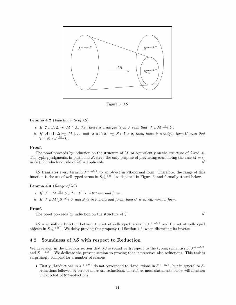
6 λS . . . . . . . . . . . . . . . . . . . . . . . . . . . . . . . . . . . . . . . . . . . . . . . . . 14

7 Translation of S→−◦&> into λ→−◦&> . . . . . . . . . . . . . . . . . . . . . . . . . . . . . . 20

8 Sλ . . . . . . . . . . . . . . . . . . . . . . . . . . . . . . . . . . . . . . . . . . . . . . . . . 22

9 Uniform Derivability . . . . . . . . . . . . . . . . . . . . . . . . . . . . . . . . . . . . . . . 30

ii

1 Introduction

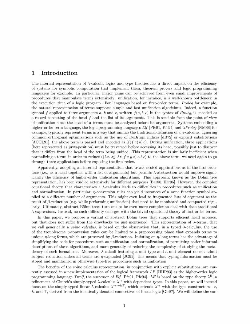
The internal representation of λ-calculi, logics and type theories has a direct impact on the efficiencyof systems for symbolic computation that implement them, theorem provers and logic programminglanguages for example. In particular, major gains can be achieved from even small improvements ofprocedures that manipulate terms extensively: unification, for instance, is a well-known bottleneck inthe execution time of a logic program. For languages based on first-order terms, Prolog for example,the natural representation of terms supports simple and fast unification algorithms. Indeed, a functionsymbol f applied to three arguments a, b and c, written f(a, b, c) in the syntax of Prolog, is encoded asa record consisting of the head f and the list of its arguments. This is sensible from the point of viewof unification since the head of a terms must be analyzed before its arguments. Systems embedding ahigher-order term language, the logic programming languages Elf [Pfe91, Pfe94] and λProlog [NM88] forexample, typically represent terms in a way that mimics the traditional definition of a λ-calculus. Ignoringcommon orthogonal optimizations such as the use of DeBruijn indices [dB72] or explicit substitutions[ACCL91], the above term is parsed and encoded as (((f a) b) c). During unification, three applications(here represented as juxtaposition) must be traversed before accessing its head, possibly just to discoverthat it differs from the head of the term being unified. This representation is similarly inefficient whennormalizing a term: in order to reduce ((λx. λy. λz. f x y z) a b c) to the above term, we need again to gothrough three applications before exposing the first redex.

Apparently, adopting an internal representation that treats nested applications as in the first-ordercase (i.e., as a head together with a list of arguments) but permits λ-abstraction would improve signif-icantly the efficiency of higher-order unification algorithms. This approach, known as the Bohm treerepresentation, has been studied extensively for different purposes [Bar80, Her95]. However, the complexequational theory that characterizes a λ-calculus leads to difficulties in procedures such as unificationand normalization. In particular, η-conversion rules can yield instances of a same function symbol ap-plied to a different number of arguments. This might even lead to fragmented lists of argument as theresult of β-reduction (e.g. while performing unification) that need to be monitored and compacted regu-larly. Ultimately, abstract Bohm trees turn out to be even more complex to deal with than traditionalλ-expressions. Instead, no such difficulty emerges with the trivial equational theory of first-order terms.

In this paper, we propose a variant of abstract Bohm trees that supports efficient head accesses,but that does not suffer from the drawbacks we just mentioned. This representation of λ-terms, thatwe call generically a spine calculus, is based on the observation that, in a typed λ-calculus, the useof the troublesome η-conversion rules can be limited to a preprocessing phase that expands terms tounique η-long forms, which are preserved by β-reduction. Insisting on η-long terms has the advantage ofsimplifying the code for procedures such as unification and normalization, of permitting easier informaldescriptions of these algorithms, and more generally of reducing the complexity of studying the meta-theory of such formalisms. Moreover, λ-calculi featuring a unit type and a unit element do not admitsubject reduction unless all terms are η-expanded [JG95]: this means that typing information must bestored and maintained in otherwise type-free procedures such as unification.

The benefits of the spine calculus representation, in conjunction with explicit substitutions, are cur-rently assessed in a new implementation of the logical framework LF [HHP93] as the higher-order logicprogramming language Twelf, the successor of Elf [Pfe91, Pfe94]. LF is based on the type theory λΠ, arefinement of Church’s simply-typed λ-calculus λ→ with dependent types. In this paper, we will insteadfocus on the simply-typed linear λ-calculus λ→−◦&>, which extends λ→ with the type constructors −◦,& and >, derived from the identically denoted connectives of linear logic [Gir87]. We will define the cor-

1

responding spine calculus S→−◦&>, present translations between the two, and prove the meta-theoreticalproperties of S→−◦&> that make it adequate as an internal representation language for λ→−◦&>. Noticethat our analysis applies to any sublanguage of λ→−◦&>, in particular to λ→ and its extension withextensional products and a unit type, λ→&>; moreover, it can easily be extended to the treatment ofdependent types.

A similar proposal for term representation was already mentioned in passing by Howard in his seminalpaper [How69]. The normal forms of the spine calculus also arise as a term assignment language foruniform proofs, which form the basis for abstract logic programming languages and is based on a muchricher set of connectives [MNPS91]. A thorough investigation of a related calculus on the λ→ fragmenthas been conducted by Herbelin [Her95]. Schwichtenberg [Sch97] studies a version of the intuitionisticspine representation and ordinary λ-calculi in a single system which incorporates permutative conversions,instead of the wholesale translation investigated here (which is closer to an efficient implementation).

λ→−◦&> corresponds, via a natural extension of the Curry-Howard isomorphism, to the (→−◦&>)fragment of intuitionistic linear logic, which constitutes the propositional core of the logic programminglanguage Lolli [HM94] and of the linear logical framework LLF [Cer96, CP96]. λ→−◦&> is also thesimply-typed variant of the term language of LLF . Its theoretical relevance derives from the fact thatit is the biggest linear λ-calculus that admits unique long βη-normal forms. λ→−◦&> shares similaritieswith the calculus proposed in [Bar96] and with the term language of the system RLF [IP96].

The implementation of a language based on a linear type theories such as LLF and RLF raisesnew challenges that do not emerge neither for intuitionistic languages such as Elf [Pfe94], nor in linearlogic programming languages featuring plain intuitionistic terms such as Lolli [HM94] or Forum [Mil94].In particular, the implementation of formalisms based on a linear λ-calculus must perform higher-orderunification on linear terms in order to instantiate existential variables [CP97]. The spine calculus S→−◦&>

was designed as an efficient representation for unification and normalization over the linear λ-expressionsthat can appear in an LLF specification.

The adoption of linear term languages in LLF and RLF has been motivated by a number of appli-cations. Linear terms provide a statically checkable notation for natural deductions [IP96] or sequentderivations [CP96] in substructural logics. In the realm of programming languages, linear terms naturallymodel computations in imperative languages [CP96] or sequences of moves in games [Cer96]. When wewant to specify, manipulate, or reason about such objects (which is common in logic and the theoryof programming languages), then internal linearity constraints are critical in practice (see, for exam-ple, the first formalizations of cut-elimination in linear logic and type preservation for Mini-ML withreferences [CP96]).

The principal contribution of this work is the definition of spine calculi (1) as a new representationtechnique for generic λ-calculi that permits both simple meta-reasoning and efficient implementations,and (2) as a term assignment system for the logic programming notion of uniform provability.

Our presentation is organized as follows. In Section 2, we define λ→−◦&> and present its mainproperties. We introduce the syntax and the typing and reduction semantics of S→−◦&> in Section 3.In Section 4, we give translations from the traditional presentation to the spine calculus and vice-versaand show that they are sound and complete with respect to the typing and reduction semantics of bothlanguages. In Section 5, we state and prove the major properties of S→−◦&>. Further remarks are madein Section 6. Finally, Section 7 summarizes the work done, discusses applications and hints at futuredevelopment. In order to facilitate our description, we must assume the reader familiar with linear logic[Gir87].

2 The Linear Simply-Typed Lambda Calculus λ→−◦&>

In this section, we introduce the linear simply-typed λ-calculus λ→−◦&>, which augments Church’s simply-typed λ-calculus λ→ [Chu40] with a number of operators from linear logic [Gir87]. More precisely, wegive its syntax in Section 2.1, present its typing semantics in Section 2.2 and its reduction semantics inSection 2.3. λ→−◦&> is the simply-typed variant of the linear type theory λΠ−◦&>, thoroughly analyzedin [Cer96]. We refer the interested reader to this work for the proofs of the properties of λ→−◦&> stated

2

Pre−canonical terms

Γ; ∆ `Σ M ↓ alλ atm

Γ; ∆ `Σ M ⇑ a

lλ unit

Γ; ∆ `Σ 〈〉 ⇑ >

Γ; ∆ `Σ M ⇑ A Γ; ∆ `Σ N ⇑ Blλ pair

Γ; ∆ `Σ 〈M,N〉 ⇑ A&B

Γ; ∆, x :A `Σ M ⇑ Blλ llam

Γ; ∆ `Σ λx :A.M ⇑ A−◦B

Γ, x :A; ∆ `Σ M ⇑ Blλ ilam

Γ; ∆ `Σ λx :A.M ⇑ A→ B. . . . . . . . . . . . . . . . . . . . . . . . . . . . . . . . . . . . . . . . . . . . . . . . . . . . . . . . . . . . . . . . . . . . . . . . . . . . . . . . . . . . . . . . . . . . . . . . . . . . . . . . . . . .Pre−atomic terms

Γ; ∆ `Σ M ⇑ Alλ redex

Γ; ∆ `Σ M ↓ Alλ con

Γ; · `Σ,c:A c ↓ Alλ lvar

Γ; x :A `Σ x ↓ Alλ ivar

Γ, x :A; · `Σ x ↓ A

(No rule for >)Γ; ∆ `Σ M ↓ A&B

lλ fst

Γ; ∆ `Σ fstM ↓ A

Γ; ∆ `Σ M ↓ A&Blλ snd

Γ; ∆ `Σ sndM ↓ B

Γ; ∆′ `Σ M ↓ A−◦B Γ; ∆′′ `Σ N ⇑ Alλ lapp

Γ; ∆′,∆′′ `Σ MˆN ↓ B

Γ; ∆ `Σ M ↓ A→ B Γ; · `Σ N ⇑ Alλ iapp

Γ; ∆ `Σ M N ↓ B

Figure 1: Typing for η-long λ→−◦&> Terms

in this section.

2.1 Syntax

The linear simply-typed λ-calculus λ→−◦&> extends Church’s λ→ with the three type constructors −◦(multiplicative arrow), & (additive product) and > (additive unit), derived from the identically denotedconnectives of linear logic. The language of terms is augmented accordingly with constructors anddestructors, devised from the natural deduction style inference rules for these connectives. Although notstrictly necessary at this level of the description, the inclusion of intuitionistic constants is convenient indevelopments of this work that go beyond the scope of this paper. We present the resulting grammar ina tabular format to relate each type constructor (left) to the corresponding term operators (center), withconstructors preceding destructors. Clearly, constants and variables can have any type.

Types: A ::= a Terms: M ::= c | x| A1 → A2 | λx :A.M | M1 M2 (intuitionistic functions)

| A1−◦A2 | λx :A.M | M1ˆM2 (linear functions)| A1 &A2 | 〈M1,M2〉 | fstM | sndM (additive pairs)| > | 〈〉 (additive unit)

Here x, c and a range over variables, constants and base types, respectively. In addition to the namesdisplayed above, we will often use N and B for terms and types, respectively.

The notions of free and bound variables are adapted from λ→. As usual, we identify terms that differonly in the name of their bound variables and write [M/x]N for the capture-avoiding substitution of Mfor x in the term N .

2.2 Typing Semantics

As usual, we rely on signatures and contexts to assign types to constants and free variables, respectively.

Signatures: Σ ::= · | Σ, c : A Contexts: Γ ::= · | Γ, x : A

3

We will also use the letter ∆, possibly subscripted, to indicate a context. Contexts and signaturesare treated as multisets; we promote “,” to denote their union and omit writing “·” when unnecessary.Finally, we require variables and constants to be declared at most once in a context and in a signature,respectively.

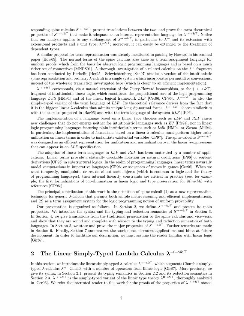
Operating solely on well-typed terms in η-long form is particularly convenient when implementingoperations such as unification since it strongly restricts the structure that a term of a given type canassume. Instead, untyped η-conversion rules are often included in the reduction semantics of a λ-calculusin order to focus on η-long representatives when needed. In the presence of a unit element, 〈〉 in λ→−◦&>,this approach is unsound. We cleanly realize the above desideratum by distinguishing a pre-canonicaltyping judgment, which validates precisely the well-typed terms of λ→−◦&> in η-long form (pre-canonicalterms), from a pre-atomic judgment, which handles intermediate stages of their construction (pre-atomicterms). These judgments are respectively denoted as follows:

Γ; ∆ `Σ M ⇑ A M is a pre-canonical term of type A in Γ; ∆ and ΣΓ; ∆ `Σ M ↓ A M is a pre-atomic term of type A in Γ; ∆ and Σ

where Γ and ∆ are called the intuitionistic and the linear context, respectively. Whenever a propertyholds uniformly for the pre-canonical and pre-atomic judgments above, we will write Γ; ∆ `Σ M ⇑↓ Aand then refer to the term M and the type A if needed. Moreover, if two or more such expressionsoccur in a statement, we assume that the arrows of the actual judgments match, unless explicitly statedotherwise.

The rules displayed in the upper part of Figure 1 validate pre-canonical termsM by deriving judgmentsof the form Γ; ∆ `Σ M ⇑ A. Rules lλ unit, lλ pair, lλ llam and lλ ilam allow the construction of termsof the form 〈〉, 〈M1,M2〉, λx :A.M , and λx :A.M , respectively. The manner they handle their contextis familiar from linear logic. Notice in particular that lλ unit is applicable with any linear contextand that the premisses of rule lλ pair share the same context, which also appears in its conclusion.Rules lλ llam and lλ ilam differ only by the nature of the assumption they add to the context in theirpremiss: linear in the case of the former, intuitionistic for the latter. The remaining rule defining thepre-canonical judgment, lλ atm, is particularly interesting since it is the reason why all terms derivablein the pre-canonical system are in η-long form. Notice that this rule can be applied only at base types.

The rules defining the pre-atomic judgment, Γ; ∆ `Σ M ↓ A, are displayed in the lower part ofFigure 1. They validate constants (rule lλ con) and linear and intuitionistic variables (rules lλ lvar andlλ ivar, respectively). They also allow the formation of the terms fstM , sndM , MˆN and M N (ruleslλ fst, lλ snd, lλ lapp and lλ iapp, respectively). The role played by linear assumptions in λ→−◦&> isparticularly evident in these rules. Indeed, an axiom rule (lλ con, lλ lvar and lλ ivar) can be appliedonly if the linear part of its context is empty, or contains just the variable to be validated, with the propertype. Linearity appears also in the elimination rule for −◦, where the linear context in the conclusionof rule lλ lapp is split and distributed among its premisses. Observe also that the linear context of theargument part of an intuitionistic application, in rule lλ iapp, is constrained to be empty. The presenceof rule lλ redex accounts for the possibility of validating terms containing β-redices, as defined below.If we remove it, only η-long β-normal (or more succinctly canonical) terms can be derived.

This formulation of the typing semantics of λ→−◦&> is the simply-typed variant of the pre-canonicalsystem which defines the semantics of the linear type theory underlying LLF [Cer96, CP96]. We directthe interested reader to these references for the proofs of the statements in this section.

If we ignore the terms and the distinction between the pre-canonical and the pre-atomic judgments,the rules in Figure 1 correspond to the specification of the familiar inference rules for the (→−◦&>)fragment of intuitionistic linear logic, ILL→−◦&> [HM94], presented in a natural deduction style. It iseasy to prove the equivalence to the usual sequent formulation. λ→−◦&> and ILL→−◦&> are related bya form of the Curry-Howard isomorphism: the terms that appear on the left of the types in the abovejudgments record the structure of a natural deduction proof for the corresponding linear formulas. Notethat the interactions of rules λ unit and λ lapp can flatten distinct proofs to the same λ→−◦&> term.

Extensionality, i.e., the property of validating only η-long terms, contributes to achieving the simpleand elegant formulation of the pre-unification algorithm for λ→−◦&> described in [CP97]. More im-portantly, this property and the subject reduction lemma below account for the possibility of omitting

4

Congruences

M −→ M ′lr pair1

〈M,N〉 −→ 〈M ′, N〉N −→ N ′

lr pair2

〈M,N〉 −→ 〈M,N ′〉

M −→ M ′lr fst

fstM −→ fstM ′

M −→ M ′lr snd

sndM −→ sndM ′

M −→ M ′lr llam

λx :A.M −→ λx :A.M ′

M −→ M ′lr lapp1

MˆN −→ M ′ˆN

N −→ N ′lr lapp2

MˆN −→ MˆN ′

M −→ M ′lr ilam

λx :A.M −→ λx :A.M ′

M −→ M ′lr iapp1

M N −→ M ′ N

N −→ N ′lr iapp2

M N −→ M N ′

. . . . . . . . . . . . . . . . . . . . . . . . . . . . . . . . . . . . . . . . . . . . . . . . . . . . . . . . . . . . . . . . . . . . . . . . . . . . . . . . . . . . . . . . . . . . . . . . . . . . . . . . . . . .β−reductions

lr beta fst

fst 〈M,N〉 −→ Mlr beta snd

snd 〈M,N〉 −→ N

lr beta lin

(λx :A.M)ˆN −→ [N/x]Mlr beta int

(λx :A.M)N −→ [N/x]M

Figure 2: Reduction Semantics for λ→−◦&>

type information in an implementation of this procedure, an essential efficiency gain. Extensionality isformalized in the following lemma, which proof can be easily adapted from [Cer96].

Lemma 2.1 (Extensionality)

i . If Γ; ∆ `Σ M ⇑ a, then M is one of c, x, fstN, sndN, N1ˆN2, N1 N2;

ii . If Γ; ∆ `Σ M ⇑ >, then M = 〈〉;iii . If Γ; ∆ `Σ M ⇑ A&B, then M = 〈N1, N2〉;iv. If Γ; ∆ `Σ M ⇑ A−◦B, then M = λx :A.N ;

v. If Γ; ∆ `Σ M ⇑ A→ B, then M = λx :A.N . 2

2.3 Reduction Semantics

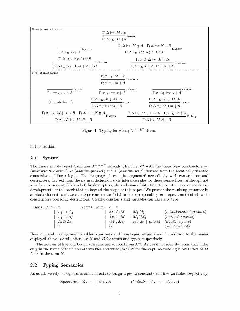
The reduction semantics of λ→−◦&> is given by the congruence relation on terms −→ based on thefollowing β-reduction rules:

βfst : fst 〈M,N〉 −→M βlapp : (λx :A.M)ˆN −→ [N/x]M

βsnd : snd 〈M,N〉 −→N βiapp : (λx :A.M)N −→ [N/x]M.

The complete definition of −→ is displayed in Figure 2. If M −→ N is derivable, then N differs fromM by the reduction of exactly one redex. We denote its reflexive and transitive closure as −→∗, and use≡ for the corresponding equivalence relation. It is easy to show that the rules obtained from Figure 2by replacing −→ with −→∗ (or even with ≡) are admissible. We adopt the standard terminology andcall a term M that does not contain β-redices normal, or β-normal. When emphasizing the fact that ourwell-typed terms are η-long, we will instead use the term canonical.

Similarly to λ→, λ→−◦&> enjoys a number of highly desirable properties [Cer96]. In particular,confluence and the Church-Rosser property hold for this language, as expressed by the following lemma:

Theorem 2.2 (Church-Rosser)

Confluence: If M −→∗ M ′ and M −→∗ M ′′, then there is a term N such thatM ′ −→∗ N and M ′′ −→∗ N .

Church-Rosser: If M ′ ≡M ′′, then there is a term N such that M ′ −→∗ N and M ′′ −→∗ N . 2

5

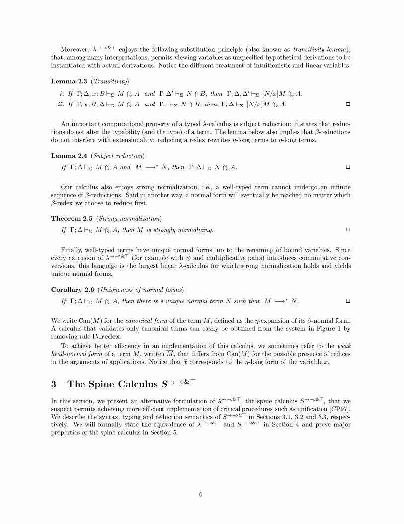
Moreover, λ→−◦&> enjoys the following substitution principle (also known as transitivity lemma),that, among many interpretations, permits viewing variables as unspecified hypothetical derivations to beinstantiated with actual derivations. Notice the different treatment of intuitionistic and linear variables.

Lemma 2.3 (Transitivity)

i . If Γ; ∆, x :B `Σ M ⇑↓ A and Γ; ∆′ `Σ N ⇑ B, then Γ; ∆,∆′ `Σ [N/x]M ⇑↓ A.

ii . If Γ, x :B; ∆ `Σ M ⇑↓ A and Γ; · `Σ N ⇑ B, then Γ; ∆ `Σ [N/x]M ⇑↓ A. 2

An important computational property of a typed λ-calculus is subject reduction: it states that reduc-tions do not alter the typability (and the type) of a term. The lemma below also implies that β-reductionsdo not interfere with extensionality: reducing a redex rewrites η-long terms to η-long terms.

Lemma 2.4 (Subject reduction)

If Γ; ∆ `Σ M ⇑↓ A and M −→∗ N , then Γ; ∆ `Σ N ⇑↓ A. 2

Our calculus also enjoys strong normalization, i.e., a well-typed term cannot undergo an infinitesequence of β-reductions. Said in another way, a normal form will eventually be reached no matter whichβ-redex we choose to reduce first.

Theorem 2.5 (Strong normalization)

If Γ; ∆ `Σ M ⇑↓ A, then M is strongly normalizing. 2

Finally, well-typed terms have unique normal forms, up to the renaming of bound variables. Sinceevery extension of λ→−◦&> (for example with ⊗ and multiplicative pairs) introduces commutative con-versions, this language is the largest linear λ-calculus for which strong normalization holds and yieldsunique normal forms.

Corollary 2.6 (Uniqueness of normal forms)

If Γ; ∆ `Σ M ⇑↓ A, then there is a unique normal term N such that M −→∗ N . 2

We write Can(M) for the canonical form of the term M , defined as the η-expansion of its β-normal form.A calculus that validates only canonical terms can easily be obtained from the system in Figure 1 byremoving rule lλ redex.

To achieve better efficiency in an implementation of this calculus, we sometimes refer to the weakhead-normal form of a term M , written M , that differs from Can(M) for the possible presence of redicesin the arguments of applications. Notice that x corresponds to the η-long form of the variable x.

3 The Spine Calculus S→−◦&>

In this section, we present an alternative formulation of λ→−◦&>, the spine calculus S→−◦&>, that wesuspect permits achieving more efficient implementation of critical procedures such as unification [CP97].We describe the syntax, typing and reduction semantics of S→−◦&> in Sections 3.1, 3.2 and 3.3, respec-tively. We will formally state the equivalence of λ→−◦&> and S→−◦&> in Section 4 and prove majorproperties of the spine calculus in Section 5.

6

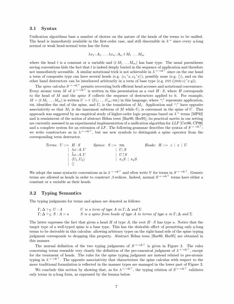
3.1 Syntax

Unification algorithms base a number of choices on the nature of the heads of the terms to be unified.The head is immediately available in the first-order case, and still discernible in λ→ since every η-longnormal or weak head-normal term has the form

λx1 :A1. . . . λxn :An. t M1 . . .Mm

where the head t is a constant or a variable and (t M1 . . .Mm) has base type. The usual parenthesessaving conventions hide the fact that t is indeed deeply buried in the sequence of application and thereforenot immediately accessible. A similar notational trick is not achievable in λ→−◦&> since on the one handa term of composite type can have several heads (e.g. 〈c1ˆx, c2ˆx〉), possibly none (e.g. 〈〉), and on theother hand destructors can be interleaved arbitrarily in a term of base type (e.g. fst ((snd c)ˆx y)).

The spine calculus S→−◦&> permits recovering both efficient head accesses and notational convenience.Every atomic term M of λ→−◦&> is written in this presentation as a root H · S, where H correspondsto the head of M and the spine S collects the sequence of destructors applied to it. For example,M = (t M1 . . .Mm) is written U = t · (U1; . . .Um; nil) in this language, where “;” represents application,nil identifies the end of the spine, and Ui is the translation of Mi. Application and “;” have oppositeassociativity so that M1 is the innermost subterm of M while U1 is outermost in the spine of U . Thisapproach was suggested by an empirical study of higher-order logic programs based on λ→ terms [MP92]and is reminiscent of the notion of abstract Bohm trees [Bar80, Her95]; its practical merits in our settingare currently assessed in an experimental implementation of a unification algorithm for LLF [Cer96, CP96]and a complete system for an extension of LF . The following grammar describes the syntax of S→−◦&>:we write constructors as in λ→−◦&>, but use new symbols to distinguish a spine operator from thecorresponding term destructor.

Terms: U ::= H · S Spines: S ::= nil Heads: H ::= c | x | U| λx :A.U | U ;S

| λx :A.U | U ;S| 〈U1, U2〉 | π1S | π2S| 〈〉

We adopt the same syntactic conventions as in λ→−◦&> and often write V for terms in S→−◦&>. Genericterms are allowed as heads in order to construct β-redices. Indeed, normal S→−◦&> terms have either aconstant or a variable as their heads.

3.2 Typing Semantics

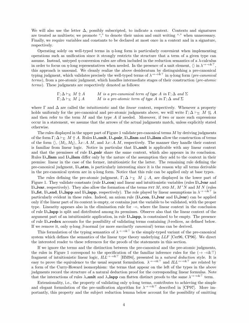
The typing judgments for terms and spines are denoted as follows:

Γ; ∆ `Σ U : A U is a term of type A in Γ; ∆ and ΣΓ; ∆ `Σ S : A > a S is a spine from heads of type A to terms of type a in Γ; ∆ and Σ

The latter expresses the fact that given a head H of type A, the root H · S has type a. Notice that thetarget type of a well-typed spine is a base type. This has the desirable effect of permitting only η-longterms to be derivable in this calculus: allowing arbitrary types on the right-hand side of the spine typingjudgment corresponds to dropping this property. Abstract Bohm trees [Bar80, Her95] are obtained inthis manner.

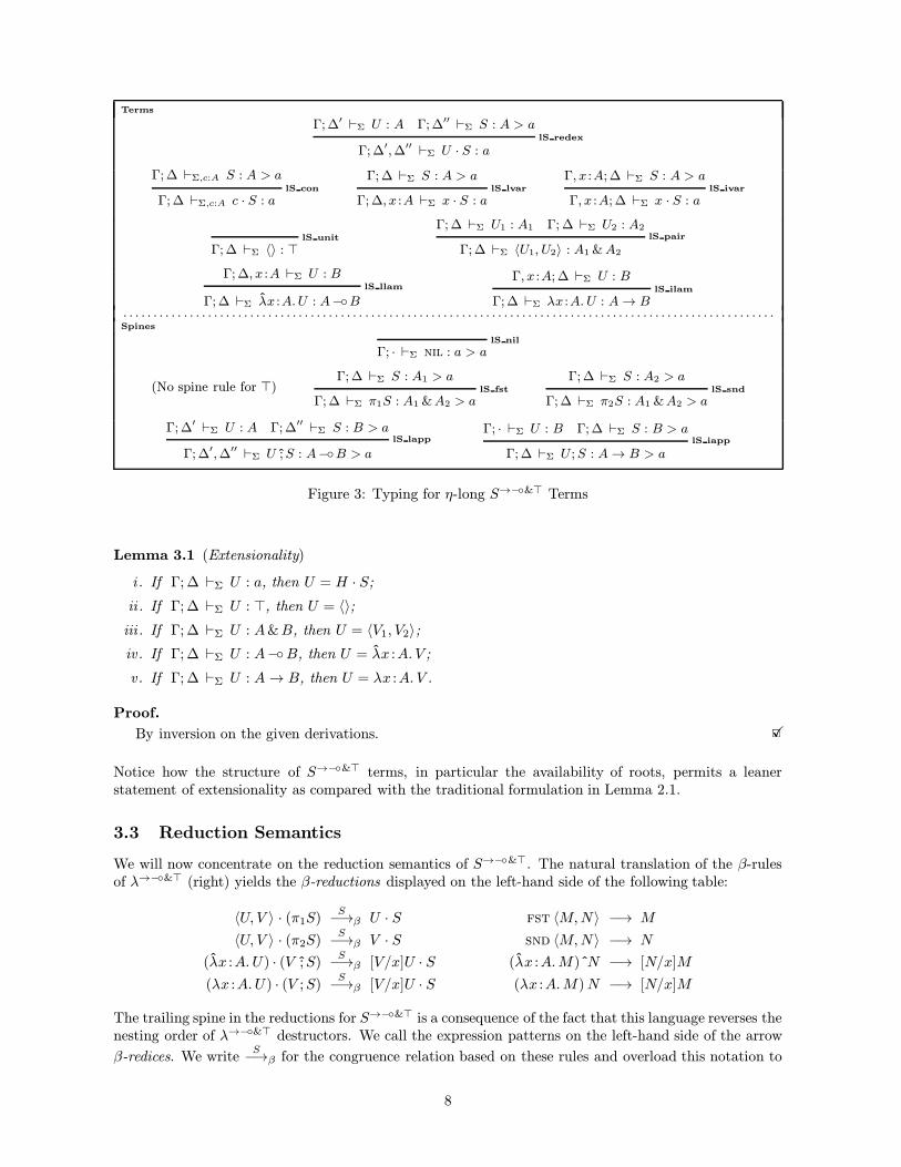
The mutual definition of the two typing judgments of S→−◦&> is given in Figure 3. The rulesconcerning terms resemble very closely the definition of the pre-canonical judgment of λ→−◦&>, exceptfor the treatment of heads. The rules for the spine typing judgment are instead related to pre-atomictyping in λ→−◦&>. The opposite associativity that characterizes the spine calculus with respect to themore traditional formulation is reflected in the manner types are managed in the lower part of Figure 3.

We conclude this section by showing that, as for λ→−◦&>, the typing relation of S→−◦&> validatesonly terms in η-long form, as expressed by the lemma below.

7

Terms

Γ; ∆′ `Σ U : A Γ; ∆′′ `Σ S : A > alS redex

Γ; ∆′,∆′′ `Σ U · S : a

Γ; ∆ `Σ,c:A S : A > alS con

Γ; ∆ `Σ,c:A c · S : a

Γ; ∆ `Σ S : A > alS lvar

Γ; ∆, x :A `Σ x · S : a

Γ, x :A; ∆ `Σ S : A > alS ivar

Γ, x :A; ∆ `Σ x · S : a

lS unit

Γ; ∆ `Σ 〈〉 : >

Γ; ∆ `Σ U1 : A1 Γ; ∆ `Σ U2 : A2lS pair

Γ; ∆ `Σ 〈U1, U2〉 : A1 &A2

Γ; ∆, x :A `Σ U : BlS llam

Γ; ∆ `Σ λx :A.U : A−◦B

Γ, x :A; ∆ `Σ U : BlS ilam

Γ; ∆ `Σ λx :A. U : A→ B. . . . . . . . . . . . . . . . . . . . . . . . . . . . . . . . . . . . . . . . . . . . . . . . . . . . . . . . . . . . . . . . . . . . . . . . . . . . . . . . . . . . . . . . . . . . . . . . . . . . . . . . . . . .Spines

lS nil

Γ; · `Σ nil : a > a

(No spine rule for >)Γ; ∆ `Σ S : A1 > a

lS fst

Γ; ∆ `Σ π1S : A1 &A2 > a

Γ; ∆ `Σ S : A2 > alS snd

Γ; ∆ `Σ π2S : A1 &A2 > a

Γ; ∆′ `Σ U : A Γ; ∆′′ `Σ S : B > alS lapp

Γ; ∆′,∆′′ `Σ U ;S : A−◦B > a

Γ; · `Σ U : B Γ; ∆ `Σ S : B > alS iapp

Γ; ∆ `Σ U ;S : A→ B > a

Figure 3: Typing for η-long S→−◦&> Terms

Lemma 3.1 (Extensionality)

i . If Γ; ∆ `Σ U : a, then U = H · S;

ii . If Γ; ∆ `Σ U : >, then U = 〈〉;iii . If Γ; ∆ `Σ U : A&B, then U = 〈V1, V2〉;iv. If Γ; ∆ `Σ U : A−◦B, then U = λx :A. V ;

v. If Γ; ∆ `Σ U : A→ B, then U = λx :A. V .

Proof.

By inversion on the given derivations. 2X

Notice how the structure of S→−◦&> terms, in particular the availability of roots, permits a leanerstatement of extensionality as compared with the traditional formulation in Lemma 2.1.

3.3 Reduction Semantics

We will now concentrate on the reduction semantics of S→−◦&>. The natural translation of the β-rulesof λ→−◦&> (right) yields the β-reductions displayed on the left-hand side of the following table:

〈U, V 〉 · (π1S)S−→β U · S fst 〈M,N〉 −→ M

〈U, V 〉 · (π2S)S−→β V · S snd 〈M,N〉 −→ N

(λx :A.U) · (V ;S)S−→β [V/x]U · S (λx :A.M)ˆN −→ [N/x]M

(λx :A.U) · (V ;S)S−→β [V/x]U · S (λx :A.M)N −→ [N/x]M

The trailing spine in the reductions for S→−◦&> is a consequence of the fact that this language reverses thenesting order of λ→−◦&> destructors. We call the expression patterns on the left-hand side of the arrow

β-redices. We writeS−→β for the congruence relation based on these rules and overload this notation to

8

Congruences terms

SS−→ S′

Sr con

c · S S−→ c · S′S

S−→ S′Sr var

x · S S−→ x · S′

US−→ U ′

Sr redex1

U · S S−→ U ′ · S

SS−→ S′

Sr redex2

U · S S−→ U · S′

US−→ U ′

Sr pair1

〈U, V 〉 S−→ 〈U ′, V 〉

VS−→ V ′

Sr pair2

〈U, V 〉 S−→ 〈U, V ′〉

US−→ U ′

Sr llam

λx :A.US−→ λx :A.U ′

US−→ U ′

Sr ilam

λx :A.US−→ λx :A. U ′

. . . . . . . . . . . . . . . . . . . . . . . . . . . . . . . . . . . . . . . . . . . . . . . . . . . . . . . . . . . . . . . . . . . . . . . . . . . . . . . . . . . . . . . . . . . . . . . . . . . . . . . . . . . .spines

SS−→ S′

Sr fst

π1SS−→ π1S

′

SS−→ S′

Sr snd

π2SS−→ π2S

′

US−→ U ′

Sr lapp1

U ;SS−→ U ′ ;S

SS−→ S′

Sr lapp2

U ;SS−→ U ;S′

US−→ U ′

Sr iapp1

U ;SS−→ U ′;S

SS−→ S′

Sr iapp2

U ;SS−→ U ;S′

. . . . . . . . . . . . . . . . . . . . . . . . . . . . . . . . . . . . . . . . . . . . . . . . . . . . . . . . . . . . . . . . . . . . . . . . . . . . . . . . . . . . . . . . . . . . . . . . . . . . . . . . . . . .nil−reduction

Sr nil

(H · S) · nilS−→ H · S

. . . . . . . . . . . . . . . . . . . . . . . . . . . . . . . . . . . . . . . . . . . . . . . . . . . . . . . . . . . . . . . . . . . . . . . . . . . . . . . . . . . . . . . . . . . . . . . . . . . . . . . . . . . .β−reductions

Sr beta fst

〈U, V 〉 · (π1S)S−→ U · S

Sr beta snd

〈U, V 〉 · (π2S)S−→ V · S

Sr beta lin

(λx :A.U) · V ;SS−→ [V/x]U · S

Sr beta int

(λx :A.U) · V ;SS−→ [V/x]U · S

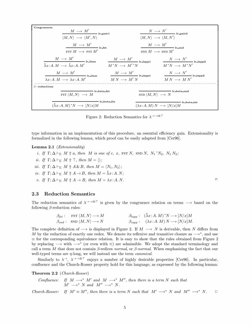
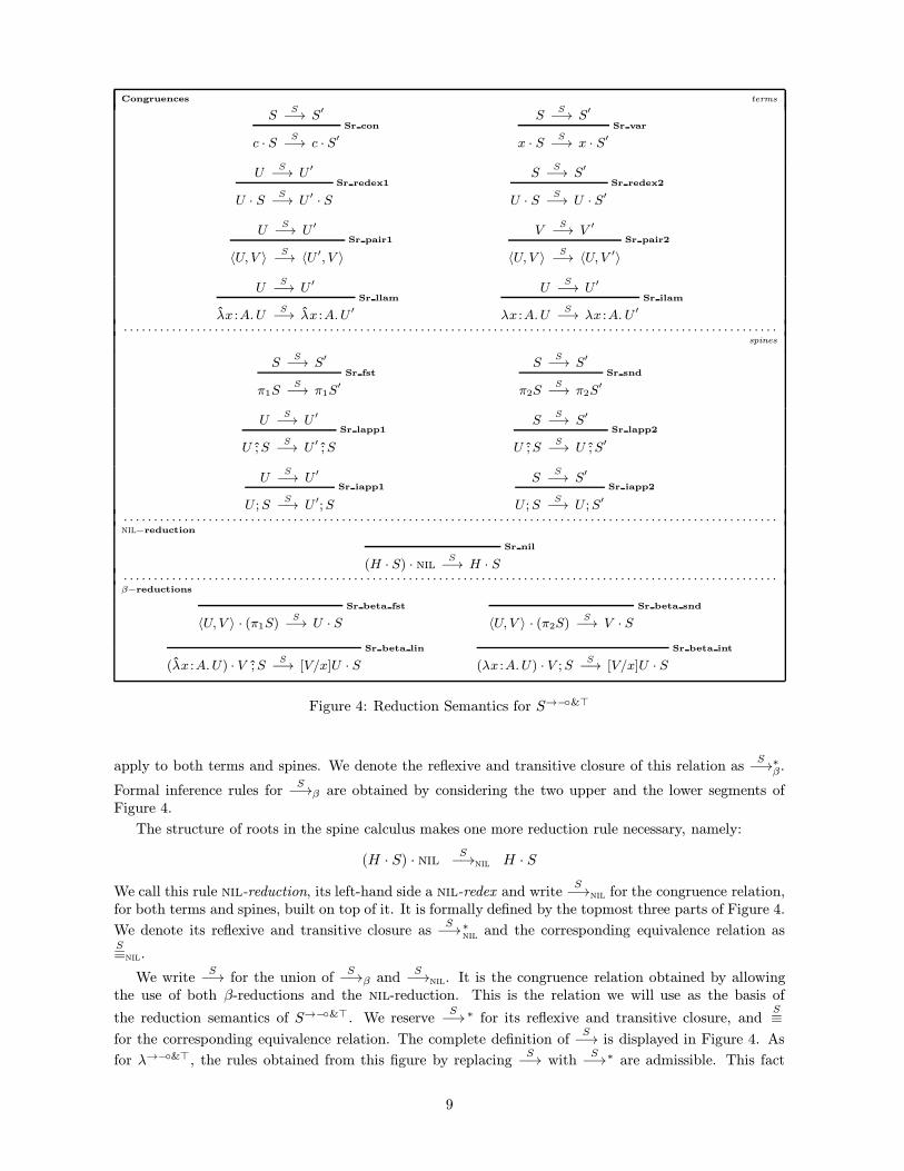
Figure 4: Reduction Semantics for S→−◦&>

apply to both terms and spines. We denote the reflexive and transitive closure of this relation asS−→∗β.

Formal inference rules forS−→β are obtained by considering the two upper and the lower segments of

Figure 4.

The structure of roots in the spine calculus makes one more reduction rule necessary, namely:

(H · S) · nilS−→nil H · S

We call this rule nil-reduction, its left-hand side a nil-redex and writeS−→nil for the congruence relation,

for both terms and spines, built on top of it. It is formally defined by the topmost three parts of Figure 4.

We denote its reflexive and transitive closure asS−→∗

niland the corresponding equivalence relation as

S≡nil.

We writeS−→ for the union of

S−→β andS−→nil. It is the congruence relation obtained by allowing

the use of both β-reductions and the nil-reduction. This is the relation we will use as the basis of

the reduction semantics of S→−◦&>. We reserveS−→ ∗ for its reflexive and transitive closure, and

S≡for the corresponding equivalence relation. The complete definition of

S−→ is displayed in Figure 4. As

for λ→−◦&>, the rules obtained from this figure by replacingS−→ with

S−→∗ are admissible. This fact

9

will enable us to lift every result below mentioningS−→ (possibly as

S−→β orS−→nil) to corresponding

properties ofS−→∗ (

S−→∗β orS−→∗

nil, respectively).

Finally, a S→−◦&> term or spine that does not contain any β- or nil-redex is called normal. Weuse instead the adjective canonical when this object is also in η-long form. By the above extensionalityproperty, every well-typed normal term is canonical.

nil-reduction appears as an omnipresent nuisance when investigating the meta-theory of S→−◦&>

in Section 5. Fortunately, we can isolate the main properties ofS−→nil and, by the very nature of the

nil-reduction, achieve simple proofs of these results. We will therefore dedicate the remainder of thissection to this task.

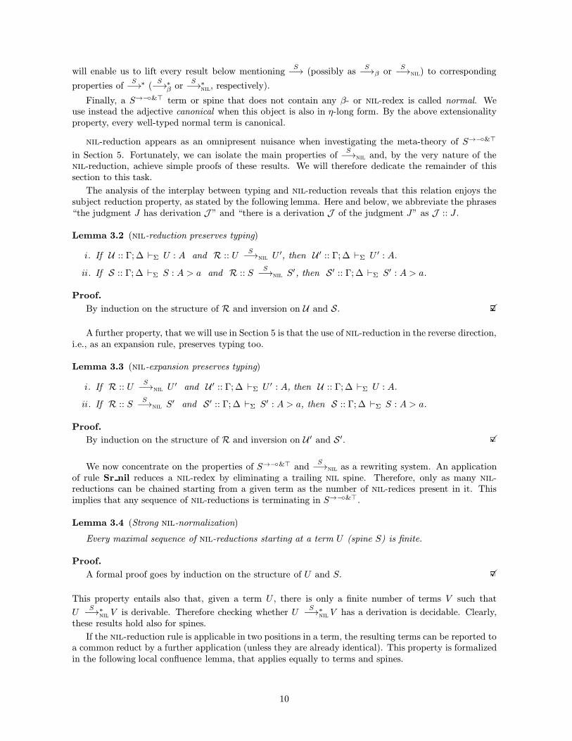
The analysis of the interplay between typing and nil-reduction reveals that this relation enjoys thesubject reduction property, as stated by the following lemma. Here and below, we abbreviate the phrases“the judgment J has derivation J ” and “there is a derivation J of the judgment J” as J :: J .

Lemma 3.2 (nil-reduction preserves typing)

i . If U :: Γ; ∆ `Σ U : A and R :: US−→nil U

′, then U ′ :: Γ; ∆ `Σ U ′ : A.

ii . If S :: Γ; ∆ `Σ S : A > a and R :: SS−→nil S

′, then S′ :: Γ; ∆ `Σ S′ : A > a.

Proof.

By induction on the structure of R and inversion on U and S. 2X

A further property, that we will use in Section 5 is that the use of nil-reduction in the reverse direction,i.e., as an expansion rule, preserves typing too.

Lemma 3.3 (nil-expansion preserves typing)

i . If R :: US−→nil U

′ and U ′ :: Γ; ∆ `Σ U ′ : A, then U :: Γ; ∆ `Σ U : A.

ii . If R :: SS−→nil S

′ and S′ :: Γ; ∆ `Σ S′ : A > a, then S :: Γ; ∆ `Σ S : A > a.

Proof.

By induction on the structure of R and inversion on U ′ and S′. 2X

We now concentrate on the properties of S→−◦&> andS−→nil as a rewriting system. An application

of rule Sr nil reduces a nil-redex by eliminating a trailing nil spine. Therefore, only as many nil-reductions can be chained starting from a given term as the number of nil-redices present in it. Thisimplies that any sequence of nil-reductions is terminating in S→−◦&>.

Lemma 3.4 (Strong nil-normalization)

Every maximal sequence of nil-reductions starting at a term U (spine S) is finite.

Proof.

A formal proof goes by induction on the structure of U and S. 2X

This property entails also that, given a term U , there is only a finite number of terms V such that

US−→∗

nilV is derivable. Therefore checking whether U

S−→∗nilV has a derivation is decidable. Clearly,

these results hold also for spines.

If the nil-reduction rule is applicable in two positions in a term, the resulting terms can be reported toa common reduct by a further application (unless they are already identical). This property is formalizedin the following local confluence lemma, that applies equally to terms and spines.

10

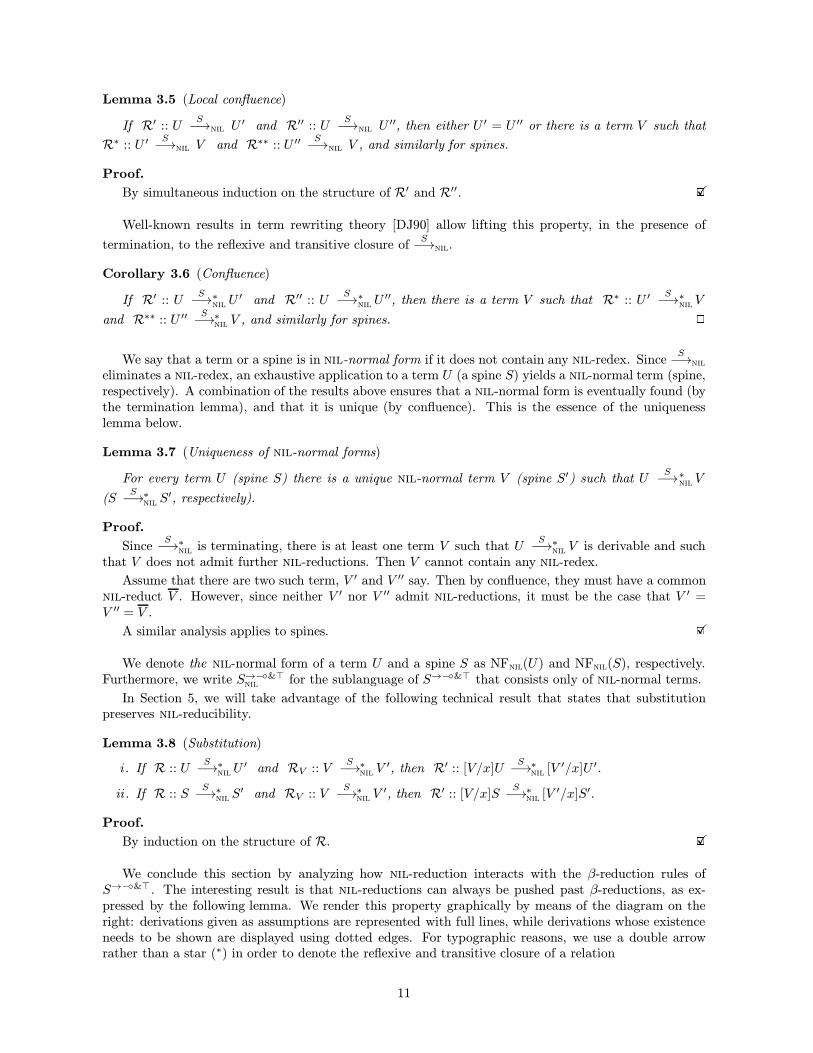
Lemma 3.5 (Local confluence)

If R′ :: US−→nil U ′ and R′′ :: U

S−→nil U ′′, then either U ′ = U ′′ or there is a term V such that

R∗ :: U ′S−→nil V and R∗∗ :: U ′′

S−→nil V , and similarly for spines.

Proof.

By simultaneous induction on the structure of R′ and R′′. 2X

Well-known results in term rewriting theory [DJ90] allow lifting this property, in the presence of

termination, to the reflexive and transitive closure ofS−→nil.

Corollary 3.6 (Confluence)

If R′ :: US−→∗

nilU ′ and R′′ :: U

S−→∗nilU ′′, then there is a term V such that R∗ :: U ′

S−→∗nilV

and R∗∗ :: U ′′S−→∗

nilV , and similarly for spines. 2

We say that a term or a spine is in nil-normal form if it does not contain any nil-redex. SinceS−→nil

eliminates a nil-redex, an exhaustive application to a term U (a spine S) yields a nil-normal term (spine,respectively). A combination of the results above ensures that a nil-normal form is eventually found (bythe termination lemma), and that it is unique (by confluence). This is the essence of the uniquenesslemma below.

Lemma 3.7 (Uniqueness of nil-normal forms)

For every term U (spine S) there is a unique nil-normal term V (spine S′) such that US−→∗

nilV

(SS−→∗

nilS′, respectively).

Proof.

SinceS−→∗

nilis terminating, there is at least one term V such that U

S−→∗nilV is derivable and such

that V does not admit further nil-reductions. Then V cannot contain any nil-redex.

Assume that there are two such term, V ′ and V ′′ say. Then by confluence, they must have a commonnil-reduct V . However, since neither V ′ nor V ′′ admit nil-reductions, it must be the case that V ′ =V ′′ = V .

A similar analysis applies to spines. 2X

We denote the nil-normal form of a term U and a spine S as NFnil(U) and NFnil(S), respectively.Furthermore, we write S→−◦&>

nilfor the sublanguage of S→−◦&> that consists only of nil-normal terms.

In Section 5, we will take advantage of the following technical result that states that substitutionpreserves nil-reducibility.

Lemma 3.8 (Substitution)

i . If R :: US−→∗

nilU ′ and RV :: V

S−→∗nilV ′, then R′ :: [V/x]U

S−→∗nil

[V ′/x]U ′.

ii . If R :: SS−→∗

nilS′ and RV :: V

S−→∗nilV ′, then R′ :: [V/x]S

S−→∗nil

[V ′/x]S′.

Proof.

By induction on the structure of R. 2X

We conclude this section by analyzing how nil-reduction interacts with the β-reduction rules ofS→−◦&>. The interesting result is that nil-reductions can always be pushed past β-reductions, as ex-pressed by the following lemma. We render this property graphically by means of the diagram on theright: derivations given as assumptions are represented with full lines, while derivations whose existenceneeds to be shown are displayed using dotted edges. For typographic reasons, we use a double arrowrather than a star (∗) in order to denote the reflexive and transitive closure of a relation

11

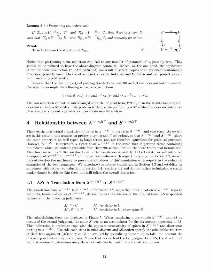
Lemma 3.9 (Postponing nil-reductions)

If Rnil :: US−→nil V ′ and Rβ :: V ′

S−→β V , then there is a term U ′

such that R′β :: US−→β U ′ and R′

nil:: U ′

S−→∗nilV , and similarly for spines.

Proof.By induction on the structure of Rnil. 2X

U V ′

U ′ V

-nil

-S

?S

β

...........-S...........-nil

-

...........?S

β

Notice that postponing a nil-reduction can lead to any number of instances of it, possibly zero. Theyshould all be reduced to have the above diagram commute. Indeed, on the one hand, the applicationof intuitionistic β-reduction (rule Sr beta int) can result in several copies of an argument containing anil-redex, possibly none. On the other hand, rules Sr beta fst and Sr beta snd can project away aterm containing a nil-redex.

Observe that the dual property of pushing β-reductions past nil-reductions does not hold in general.Consider for example the following sequence of reductions:

〈c · nil, d · nil〉 · (π1nil)S−→β (c · nil) · nil

S−→nil c · nil

The two reduction cannot be interchanged since the original term, fst 〈c, d〉 in the traditional notation,does not contain a nil-redex. The problem is that, while performing a nil-reduction does not introduceβ-redices, carrying out a β-reduction can create new nil-redices.

4 Relationship between λ→−◦&> and S→−◦&>

There exists a structural translation of terms in λ→−◦&> to terms in S→−◦&> and vice versa. As we willsee in this section, this translation preserves typing and β-reductions, so that λ→−◦&> and S→−◦&> sharethe same properties on well-typed (η-long) terms, and are therefore equivalent for practical purposes.However, S→−◦&> is structurally richer than λ→−◦&> in the sense that it permits terms containingnil-redices, which are indistinguishable from their nil-normal form in the more traditional formulation.Therefore, we will treat the two directions of the translation separately. In Section 4.1 we will introducea mapping of λ→−◦&> to S→−◦&> and prove its soundness with respect to typing. In Section 4.2, we willinstead develop the machinery to prove the soundness of this translation with respect to the reductionsemantics of the two languages. We introduce the reverse translation in Section 4.3 and establish itssoundness with respect to reduction in Section 4.4. Sections 4.2 and 4.4 are rather technical; the casualreader should be able to skip them and still follow the overall discussion.

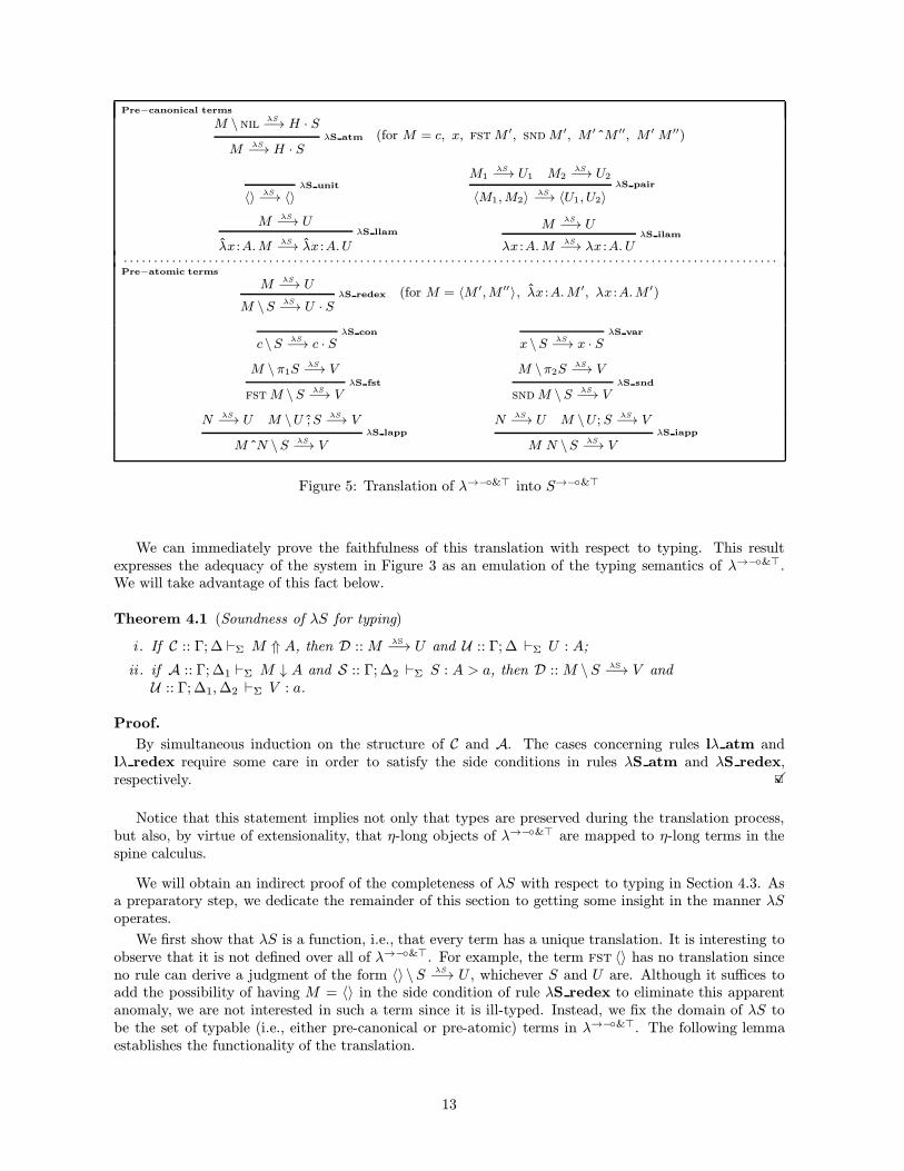
4.1 λS: A Translation from λ→−◦&> to S→−◦&>

The translation from λ→−◦&> to S→−◦&>, abbreviated λS, maps the uniform notion of λ→−◦&> term tothe roots, terms and spines of S→−◦&>, depending on the structure of the original term. λS is specifiedby means of the following judgments:

M λS−→ U M translates to UM \S λS−→ U M translates to U , given spine S

The rules defining them are displayed in Figure 5. When translating a pre-atomic λ→−◦&> term M bymeans of the second judgment, the spine S acts as an accumulator for the destructors appearing in M .This indirection is needed to cope with the opposite associativity of spines in S→−◦&> and destructornesting in λ→−◦&>. The side conditions in rules λS atm and λS redex specify the admissible structureof their first argument (M); they could be avoided by specializing these rules to take into account thedifferent possibilities they encompass. Notice that, for each of the two judgments of λS, the structure ofthe first argument determines uniquely which rule can be used in the translation process.

12

Pre−canonical terms

M \nilλS−→ H · S

λS atm

M λS−→ H · S(for M = c, x, fstM ′, sndM ′, M ′ˆM ′′, M ′M ′′)

λS unit

〈〉 λS−→ 〈〉M1

λS−→ U1 M2λS−→ U2

λS pair

〈M1,M2〉 λS−→ 〈U1, U2〉

M λS−→ UλS llam

λx :A.M λS−→ λx :A.U

MλS−→ U

λS ilam

λx :A.M λS−→ λx :A. U. . . . . . . . . . . . . . . . . . . . . . . . . . . . . . . . . . . . . . . . . . . . . . . . . . . . . . . . . . . . . . . . . . . . . . . . . . . . . . . . . . . . . . . . . . . . . . . . . . . . . . . . . . . .Pre−atomic terms

M λS−→ UλS redex

M \S λS−→ U · S(for M = 〈M ′,M ′′〉, λx :A.M ′, λx :A.M ′)

λS con

c \S λS−→ c · SλS var

x \S λS−→ x · S

M \ π1SλS−→ V

λS fst

fstM \S λS−→ V

M \π2SλS−→ V

λS snd

sndM \S λS−→ V

N λS−→ U M \U ;S λS−→ VλS lapp

MˆN \S λS−→ V

N λS−→ U M \U ; S λS−→ VλS iapp

M N \S λS−→ V

Figure 5: Translation of λ→−◦&> into S→−◦&>

We can immediately prove the faithfulness of this translation with respect to typing. This resultexpresses the adequacy of the system in Figure 3 as an emulation of the typing semantics of λ→−◦&>.We will take advantage of this fact below.

Theorem 4.1 (Soundness of λS for typing)

i . If C :: Γ; ∆ `Σ M ⇑ A, then D :: M λS−→ U and U :: Γ; ∆ `Σ U : A;

ii . if A :: Γ; ∆1 `Σ M ↓ A and S :: Γ; ∆2 `Σ S : A > a, then D :: M \S λS−→ V andU :: Γ; ∆1,∆2 `Σ V : a.

Proof.

By simultaneous induction on the structure of C and A. The cases concerning rules lλ atm andlλ redex require some care in order to satisfy the side conditions in rules λS atm and λS redex,respectively. 2X

Notice that this statement implies not only that types are preserved during the translation process,but also, by virtue of extensionality, that η-long objects of λ→−◦&> are mapped to η-long terms in thespine calculus.

We will obtain an indirect proof of the completeness of λS with respect to typing in Section 4.3. Asa preparatory step, we dedicate the remainder of this section to getting some insight in the manner λSoperates.

We first show that λS is a function, i.e., that every term has a unique translation. It is interesting toobserve that it is not defined over all of λ→−◦&>. For example, the term fst 〈〉 has no translation sinceno rule can derive a judgment of the form 〈〉 \S λS−→ U , whichever S and U are. Although it suffices toadd the possibility of having M = 〈〉 in the side condition of rule λS redex to eliminate this apparentanomaly, we are not interested in such a term since it is ill-typed. Instead, we fix the domain of λS tobe the set of typable (i.e., either pre-canonical or pre-atomic) terms in λ→−◦&>. The following lemmaestablishes the functionality of the translation.

13

λ→−◦&> S→−◦&>

S→−◦&>nil

λS

Figure 6: λS

Lemma 4.2 (Functionality of λS)

i . If C :: Γ; ∆ `Σ M ⇑ A, then there is a unique term U such that T :: M λS−→ U .

ii . If A :: Γ; ∆ `Σ M ↓ A and S :: Γ; ∆′ `Σ S : A > a, then, there is a unique term U such thatT :: M \S λS−→ U .

Proof.

The proof proceeds by induction on the structure of M , or equivalently on the structure of C and A.The typing judgments, in particular S, serve the only purpose of preventing considering the case M = 〈〉in (ii), for which no rule of λS is applicable. 2X

λS translates every term in λ→−◦&> to an object in nil-normal form. Therefore, the range of thisfunction is the set of well-typed terms in S→−◦&>

nil, as depicted in Figure 6, and formally stated below.

Lemma 4.3 (Range of λS)

i . If T :: M λS−→ U , then U is in nil-normal form.

ii . If T :: M \S λS−→ U and S is in nil-normal form, then U is in nil-normal form.

Proof.

The proof proceeds by induction on the structure of T . 2X

λS is actually a bijection between the set of well-typed terms in λ→−◦&> and the set of well-typedobjects in S→−◦&>

nil. We delay proving this property till Section 4.3, when discussing its inverse.

4.2 Soundness of λS with respect to Reduction

We have seen in the previous section that λS is sound with respect to the typing semantics of λ→−◦&>

and S→−◦&>. We dedicate the present section to proving that it preserves also reductions. This task issurprisingly complex for a number of reasons.

• Firstly, β-reductions in λ→−◦&> do not correspond to β-reductions in S→−◦&>, but in general to β-reductions followed by zero or more nil-reductions. Therefore, most statements below will mentionunexpected of nil-reductions.

14

• Secondly, the reduction semantics of S→−◦&> is specialized to η-long forms. Consider for examplethe λ→−◦&> term

M = (λx :a. f x) c d

for appropriate declarations of f , c and d (the latter two of base type). This term is not in η-longform (its η-expansion is (λx :a. λy :a′. f x y) c d). M reduces to the canonical form

N = f c d

which translation in S→−◦&> is

V = f · ((c · nil); (d · nil); nil)

On the other hand, λS would translate M to the S→−◦&> term

U = (λx :a. f · (x · nil); nil) · ((c · nil); (d · nil); nil)

which cannot be reduced further than

(f · (c · nil); nil) · ((d · nil); nil),

a different term from V . V can however be recovered by appending the spines. Such a step provedcompulsory in the implementation of LF as the new programming language Twelf. Indeed, typesleft implicit by the user are reconstructed through unification, but since not all typing informationis available at this stage, η-long forms cannot be achieved. Therefore, this preprocessing phasecannot take advantage of the strong invariants that derive from extensionality. In particular, spinesoccasionally need to be appended.

As we can see from this example, λS does not commute with reduction in the general case. We cantrack the problem to the fact that, while β-reduction and extensionality are orthogonal conceptsin λ→−◦&>, they are intimately related in S→−◦&>. Indeed, analyzing the spine calculus in theabsence of extensionality requirements reveals the nil-reduction rule as the degenerated form of ageneral η-expansion rule.

However, as long as we are interested only in η-long terms, the definitions given in the previoussection ensure the λS is sound with respect to the reduction semantics of our calculi. Therefore,we need to pay particular attention to operating only on η-long terms. We achieve this purposeindirectly by requiring explicitly that all the λ→−◦&> terms we consider be well-typed. This isstricter than needed, but typing is the only way we can enforce extensionality.

Rules lr beta lin and lr beta int generate their reduct means of a meta-level substitution. Thecorresponding reduction in S→−◦&> operate in a similar way. Therefore, we need to show that λScommutes reasonably well with substitution. This is achieved in the following lemma, where “reasonablywell” means modulo nil-reductions.

Lemma 4.4 (Substitution in λS)

i . Assume that C :: Γ; ∆ `Σ M ⇑ A, CN :: Γ; ∆′′ `Σ N ⇑ B and x :B occurs in either Γ or ∆.

If T :: M λS−→ U and TN :: N λS−→ V , then T ′ :: [N/x]M λS−→ V ′ where R :: [V/x]US−→∗

nilV ′.

ii . Assume that C :: Γ; ∆ `Σ M ↓ A, S :: Γ; ∆′′ `Σ S : A > a, CN :: Γ; ∆′ `Σ N ⇑ B and x :Boccurs in either Γ, ∆ or ∆′′.

If T :: M \S λS−→ U and TN :: N λS−→ V , then T ′ :: [N/x]M \ [V/x]S λS−→ V ′ where

R :: [V/x]US−→∗

nilV ′.

Proof.

The proof proceeds by induction on the structure of T and then by case distinction on the structureof CN . All cases are quite simple except for the situation where M is precisely x (subcase of rule λS var

15

in part (ii) of this lemma). We will analyze this situation in detail since a similar proof pattern willappear again further.

Assume therefore thatT = λS var

x \S λS−→ x · SThus, M = x, U = x · S, B = A, C is either lλ lvar, lλ ivar, or exposes one of them after traversingalternations of instances of lλ redex and lλ atm, and CN :: Γ; ∆′ `Σ N ⇑ A.

We make a case distinction on the last rule applied in CN :

Subcase lλ atm

Then, A = a′ for some base type a′. By inversion on S, we deduce that a′ = a and S = nil. Byextensionality, we further obtain that N = c, N = y, N = fstN ′, N = sndN ′, N = N ′ˆN ′′ orN = N ′ N ′′.

By inversion on rule λS atm for TN , we have that V = HV · SV and that there is a derivation T ′of N \nil

λS−→ (HV · SV ), i.e., of [N/x]x \ [V/x]nilλS−→ (HV · SV ). Now simply set R to

Sr beta nil

(HV · SV ) · nilS−→nil HV · SV

as a derivation of [V/x](x · nil)S−→∗

nilV .

Subcase lλ unit

Then, A = >, but no rule can start a derivation of Γ; ∆′′ `Σ S : > > a. Therefore, this case cannotpossibly arise.

Other subcases

By inversion, N = 〈N1, N2〉, N = λy : A′. N ′ or N = λy : A′. N ′. We apply rule λS redex toTN :: N λS−→ V to obtain a derivation T ′ of N \ [V/x]S λS−→ V · [V/x]S, i.e., of[N/x]x \ [V/x]S λS−→ [V/x](x · S). Simply take the identity as R. 2X

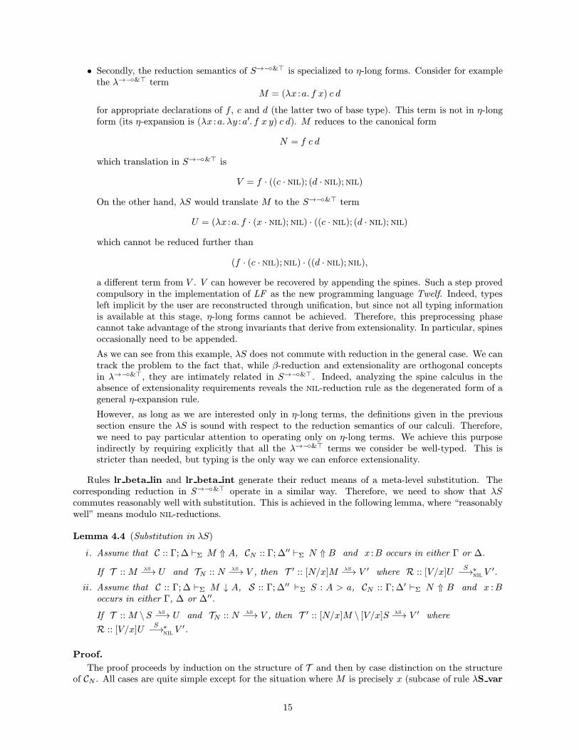
We need one more technical result prior to tackling the main theorem of this section. More precisely,we need to show that, when translating a pre-atomic term, reductions to the accessory spine are mappeddirectly to reductions in the resulting S→−◦&> term, as expressed by the diagram on the right. Inparticular, β-reductions are mapped to β-reductions and nil-reductions yield nil-reductions. Notice thatthe statement below does not mention typing derivations. Indeed it applies to generic terms, possiblyill-typed or not in η-long form.

Lemma 4.5 (Spine reduction)

i . If T :: M \S λS−→ V and R :: SS−→β S′, then there is a term

V ′ such that T ′ :: M \S′ λS−→ V ′ and R′ :: VS−→β V ′.

ii . If T :: M \S λS−→ V and R :: SS−→nil S

′, then there is a term

V ′ such that T ′ :: M \S′ λS−→ V ′ and R′ :: VS−→nil V

′.

M \ S

M \ S′

V

V ′

-λS

?S

...........-λS

...........?S

Proof.

This straightforward proof proceeds by induction on the structure of R. 2X

It is easy to show that this result remains valid when considering the transitive and reflexive closure of

the involved relations, or evenS−→∗.

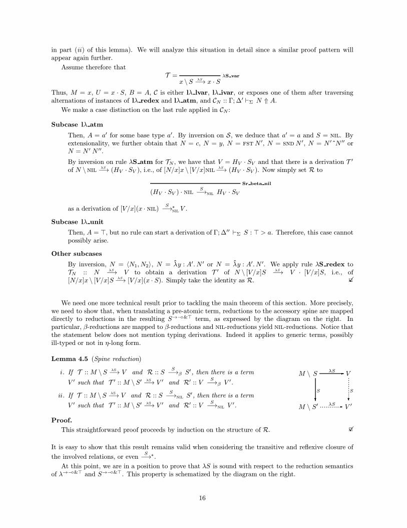
At this point, we are in a position to prove that λS is sound with respect to the reduction semanticsof λ→−◦&> and S→−◦&>. This property is schematized by the diagram on the right.

16

Theorem 4.6 (Soundness of λS for reducibility)

i . Assume that C :: Γ; ∆ `Σ M ⇑ A.

If R :: M −→ N and T :: M λS−→ U , then there are terms

V and V such that Rβ :: US−→β V , Rnil :: V

S−→∗nilV and

T ′ :: N λS−→ V .

M

U

N

V V

-

?λS

................R

λS

............-S............-β

...........-S...........-nil

-

ii . Assume that A :: Γ; ∆1 `Σ M ↓ A and S :: Γ; ∆2 `Σ S : A > a.

If R :: M −→ N and T :: M \S λS−→ U , then there are terms V and V such that

Rβ :: US−→β V , Rnil :: V

S−→∗nilV and T ′ :: N \S λS−→ V .

Proof.

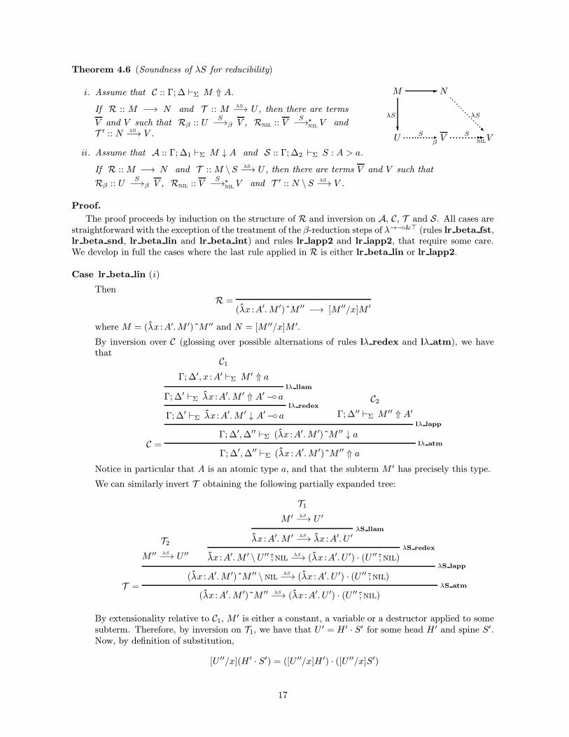
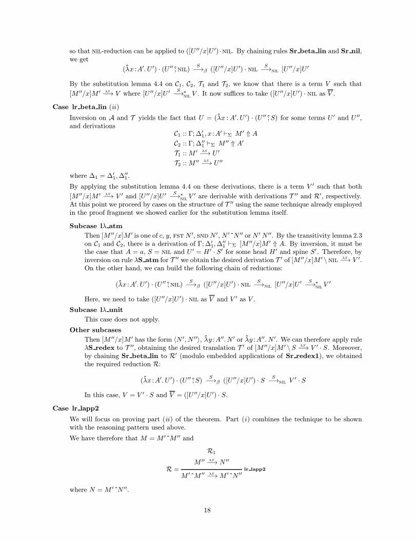
The proof proceeds by induction on the structure of R and inversion on A, C, T and S. All cases arestraightforward with the exception of the treatment of the β-reduction steps of λ→−◦&> (rules lr beta fst,lr beta snd, lr beta lin and lr beta int) and rules lr lapp2 and lr iapp2, that require some care.We develop in full the cases where the last rule applied in R is either lr beta lin or lr lapp2.

Case lr beta lin (i)

ThenR =

(λx :A′.M ′)ˆM ′′ −→ [M ′′/x]M ′

where M = (λx :A′.M ′)ˆM ′′ and N = [M ′′/x]M ′.

By inversion over C (glossing over possible alternations of rules lλ redex and lλ atm), we havethat

C =

C1Γ; ∆′, x :A′ `Σ M ′ ⇑ a

lλ llam

Γ; ∆′ `Σ λx :A′.M ′ ⇑ A′−◦ alλ redex

Γ; ∆′ `Σ λx :A′.M ′ ↓ A′−◦ aC2

Γ; ∆′′ `Σ M ′′ ⇑ A′lλ lapp

Γ; ∆′,∆′′ `Σ (λx :A′.M ′)ˆM ′′ ↓ alλ atm

Γ; ∆′,∆′′ `Σ (λx :A′.M ′)ˆM ′′ ⇑ aNotice in particular that A is an atomic type a, and that the subterm M ′ has precisely this type.

We can similarly invert T obtaining the following partially expanded tree:

T =

T2

M ′′ λS−→ U ′′

T1

M ′ λS−→ U ′

λS llam

λx :A′.M ′ λS−→ λx :A′. U ′

λS redex

λx :A′.M ′ \U ′′ ; nilλS−→ (λx :A′. U ′) · (U ′′ ; nil)

λS lapp

(λx :A′.M ′)ˆM ′′ \nilλS−→ (λx :A′. U ′) · (U ′′ ; nil)

λS atm

(λx :A′.M ′)ˆM ′′ λS−→ (λx :A′. U ′) · (U ′′ ; nil)

By extensionality relative to C1, M ′ is either a constant, a variable or a destructor applied to somesubterm. Therefore, by inversion on T1, we have that U ′ = H ′ · S′ for some head H ′ and spine S′.Now, by definition of substitution,

[U ′′/x](H ′ · S′) = ([U ′′/x]H ′) · ([U ′′/x]S′)

17

so that nil-reduction can be applied to ([U ′′/x]U ′) ·nil. By chaining rules Sr beta lin and Sr nil,we get

(λx :A′. U ′) · (U ′′ ; nil)S−→β ([U ′′/x]U ′) · nil

S−→nil [U ′′/x]U ′

By the substitution lemma 4.4 on C1, C2, T1 and T2, we know that there is a term V such that

[M ′′/x]M ′ λS−→ V where [U ′′/x]U ′S−→∗

nilV . It now suffices to take ([U ′′/x]U ′) · nil as V .

Case lr beta lin (ii)

Inversion on A and T yields the fact that U = (λx :A′. U ′) · (U ′′ ;S) for some terms U ′ and U ′′,and derivations

C1 :: Γ; ∆′1, x :A′ `Σ M ′ ⇑ AC2 :: Γ; ∆′′1 `Σ M ′′ ⇑ A′

T1 :: M ′ λS−→ U ′

T2 :: M ′′ λS−→ U ′′

where ∆1 = ∆′1,∆′′1.

By applying the substitution lemma 4.4 on these derivations, there is a term V ′ such that both

[M ′′/x]M ′ λS−→ V ′ and [U ′′/x]U ′S−→∗

nilV ′ are derivable with derivations T ′′ and R′, respectively.

At this point we proceed by cases on the structure of T ′′ using the same technique already employedin the proof fragment we showed earlier for the substitution lemma itself.

Subcase lλ atm

Then [M ′′/x]M ′ is one of c, y, fstN ′, sndN ′, N ′ˆN ′′ orN ′ N ′′. By the transitivity lemma 2.3on C1 and C2, there is a derivation of Γ; ∆′1,∆

′′1 `Σ [M ′′/x]M ′ ⇑ A. By inversion, it must be

the case that A = a, S = nil and U ′ = H ′ · S′ for some head H ′ and spine S′. Therefore, byinversion on rule λS atm for T ′′ we obtain the desired derivation T ′ of [M ′′/x]M ′ \nil

λS−→ V ′.On the other hand, we can build the following chain of reductions:

(λx :A′. U ′) · (U ′′ ; nil)S−→β ([U ′′/x]U ′) · nil

S−→nil [U ′′/x]U ′S−→∗

nilV ′

Here, we need to take ([U ′′/x]U ′) · nil as V and V ′ as V .

Subcase lλ unit

This case does not apply.

Other subcases

Then [M ′′/x]M ′ has the form 〈N ′, N ′′〉, λy :A′′. N ′ or λy :A′′. N ′. We can therefore apply ruleλS redex to T ′′, obtaining the desired translation T ′ of [M ′′/x]M ′ \S λS−→ V ′ · S. Moreover,by chaining Sr beta lin to R′ (modulo embedded applications of Sr redex1), we obtainedthe required reduction R:

(λx :A′. U ′) · (U ′′ ;S)S−→β ([U ′′/x]U ′) · S S−→nil V

′ · S

In this case, V = V ′ · S and V = ([U ′′/x]U ′) · S.

Case lr lapp2

We will focus on proving part (ii) of the theorem. Part (i) combines the technique to be shownwith the reasoning pattern used above.

We have therefore that M = M ′ˆM ′′ and

R =

R1

M ′′ λS−→ N ′′

lr lapp2

M ′ˆM ′′ λS−→M ′ˆN ′′

where N = M ′ˆN ′′.

18

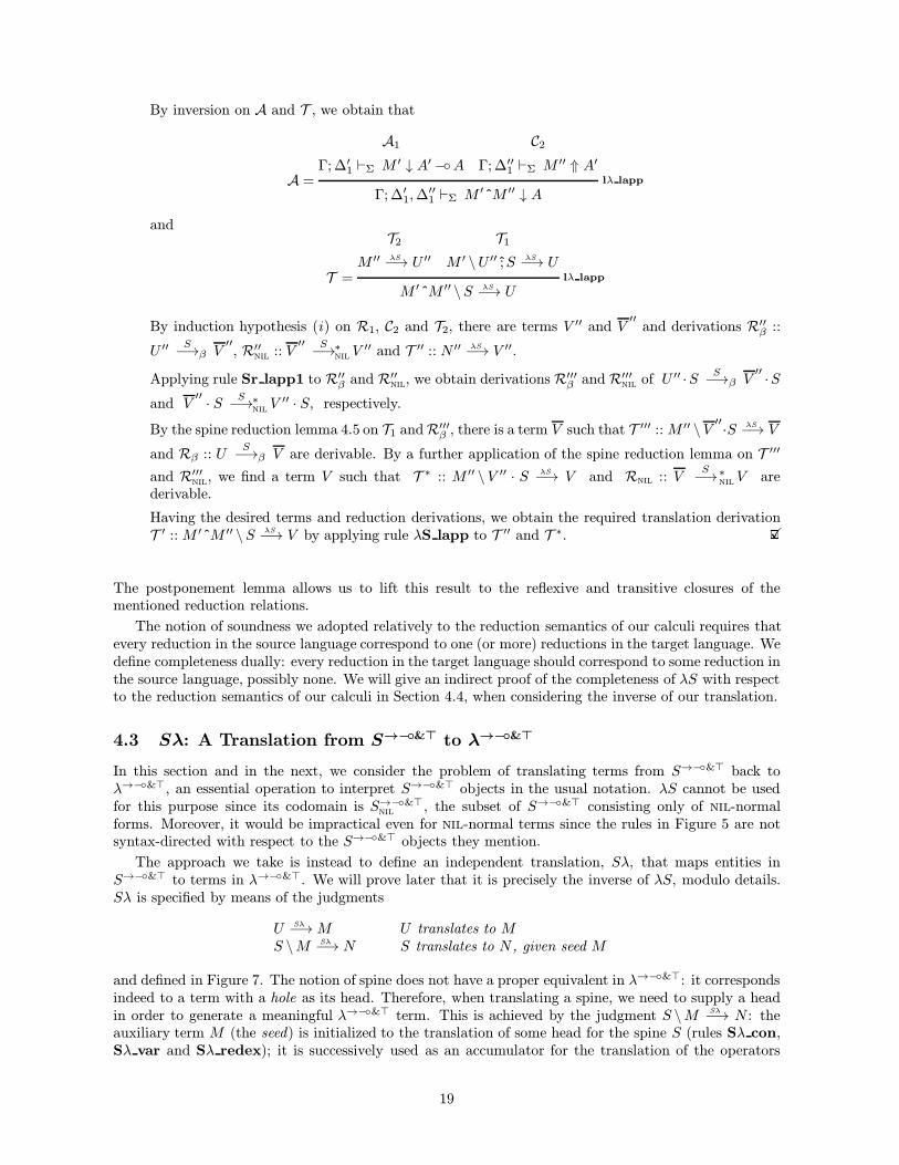
By inversion on A and T , we obtain that

A =

A1

Γ; ∆′1 `Σ M ′ ↓ A′−◦AC2

Γ; ∆′′1 `Σ M ′′ ⇑ A′lλ lapp

Γ; ∆′1,∆′′1 `Σ M ′ˆM ′′ ↓ A

and

T =

T2

M ′′ λS−→ U ′′T1

M ′ \U ′′ ;S λS−→ Ulλ lapp

M ′ˆM ′′ \S λS−→ U

By induction hypothesis (i) on R1, C2 and T2, there are terms V ′′ and V′′

and derivations R′′β ::

U ′′S−→β V

′′, R′′

nil:: V

′′ S−→∗nilV ′′ and T ′′ :: N ′′ λS−→ V ′′.

Applying rule Sr lapp1 to R′′β and R′′nil

, we obtain derivations R′′′β and R′′′nil

of U ′′ ·S S−→β V′′ ·S

and V′′ · S S−→∗

nilV ′′ · S, respectively.

By the spine reduction lemma 4.5 on T1 andR′′′β , there is a term V such that T ′′′ :: M ′′ \V ′′·S λS−→ V

and Rβ :: US−→β V are derivable. By a further application of the spine reduction lemma on T ′′′

and R′′′nil

, we find a term V such that T ∗ :: M ′′ \V ′′ · S λS−→ V and Rnil :: VS−→∗

nilV are

derivable.

Having the desired terms and reduction derivations, we obtain the required translation derivationT ′ :: M ′ˆM ′′ \S λS−→ V by applying rule λS lapp to T ′′ and T ∗. 2X

The postponement lemma allows us to lift this result to the reflexive and transitive closures of thementioned reduction relations.

The notion of soundness we adopted relatively to the reduction semantics of our calculi requires thatevery reduction in the source language correspond to one (or more) reductions in the target language. Wedefine completeness dually: every reduction in the target language should correspond to some reduction inthe source language, possibly none. We will give an indirect proof of the completeness of λS with respectto the reduction semantics of our calculi in Section 4.4, when considering the inverse of our translation.

4.3 Sλ: A Translation from S→−◦&> to λ→−◦&>

In this section and in the next, we consider the problem of translating terms from S→−◦&> back toλ→−◦&>, an essential operation to interpret S→−◦&> objects in the usual notation. λS cannot be usedfor this purpose since its codomain is S→−◦&>

nil, the subset of S→−◦&> consisting only of nil-normal

forms. Moreover, it would be impractical even for nil-normal terms since the rules in Figure 5 are notsyntax-directed with respect to the S→−◦&> objects they mention.

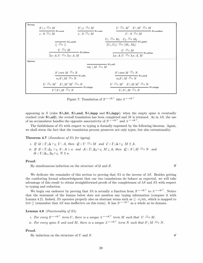
The approach we take is instead to define an independent translation, Sλ, that maps entities inS→−◦&> to terms in λ→−◦&>. We will prove later that it is precisely the inverse of λS, modulo details.Sλ is specified by means of the judgments

U Sλ−→M U translates to MS \M Sλ−→ N S translates to N , given seed M

and defined in Figure 7. The notion of spine does not have a proper equivalent in λ→−◦&>: it correspondsindeed to a term with a hole as its head. Therefore, when translating a spine, we need to supply a headin order to generate a meaningful λ→−◦&> term. This is achieved by the judgment S \M Sλ−→ N : theauxiliary term M (the seed) is initialized to the translation of some head for the spine S (rules Sλ con,Sλ var and Sλ redex); it is successively used as an accumulator for the translation of the operators

19

Terms

S \ c Sλ−→MSλ con

c · S Sλ−→ M

S \x Sλ−→MSλ var

x · S Sλ−→M

U Sλ−→M ′ S \M ′ Sλ−→MSλ redex

U · S Sλ−→M

Sλ unit

〈〉 Sλ−→ 〈〉U1

Sλ−→M1 U2Sλ−→M2

Sλ pair

〈U1, U2〉 Sλ−→ 〈M1,M2〉

U Sλ−→MSλ llam

λx :A.U Sλ−→ λx :A.M

U Sλ−→MSλ ilam

λx :A.U Sλ−→ λx :A.M. . . . . . . . . . . . . . . . . . . . . . . . . . . . . . . . . . . . . . . . . . . . . . . . . . . . . . . . . . . . . . . . . . . . . . . . . . . . . . . . . . . . . . . . . . . . . . . . . . . . . . . . . . . .Spines

Sλ nil

nil \M Sλ−→M

S \fstMSλ−→ N

Sλ fst

π1S \M Sλ−→ N

S \ sndMSλ−→ N

Sλ snd

π2S \M Sλ−→ N

U Sλ−→M ′ S \MˆM ′ Sλ−→ NSλ lapp

U ;S \M Sλ−→ N

U Sλ−→M ′ S \M M ′ Sλ−→ NSλ iapp

U ;S \M Sλ−→ N

Figure 7: Translation of S→−◦&> into λ→−◦&>

appearing in S (rules Sλ fst, Sλ snd, Sλ lapp and Sλ iapp); when the empty spine is eventuallyreached (rule Sλ nil), the overall translation has been completed and M is returned. As in λS, the useof an accumulator handles the opposite associativity of S→−◦&> and λ→−◦&>.

The faithfulness of Sλ with respect to typing is formally expressed by the following theorem. Again,we shall stress the fact that the translation process preserves not only types, but also extensionality.

Theorem 4.7 (Soundness of Sλ for typing)

i . If U :: Γ; ∆ `Σ U : A, then Q :: U Sλ−→M and C :: Γ; ∆ `Σ M ⇑ A.

ii . If S :: Γ; ∆1 `Σ S : A > a and A :: Γ; ∆2 `Σ M ↓ A, then Q :: S \M Sλ−→ N andU :: Γ; ∆1,∆2 `Σ N ⇑ a.

Proof.

By simultaneous induction on the structure of U and S. 2X

We dedicate the remainder of this section to proving that Sλ is the inverse of λS. Besides gettingthe comforting formal acknowledgment that our two translations do behave as expected, we will takeadvantage of this result to obtain straightforward proofs of the completeness of λS and Sλ with respectto typing and reduction.

We begin our endeavor by proving that Sλ is actually a function from S→−◦&> to λ→−◦&>. Noticethat the statement of the lemma below does not mention any typing information (compare it withLemma 4.2). Indeed, Sλ operates properly also on aberrant terms such as 〈〉 · π1nil, which is mapped tofst 〈〉 (remember that λS was ineffective on this term). It has S→−◦&> as a whole as its domain.

Lemma 4.8 (Functionality of Sλ)

i . For every S→−◦&> term U , there is a unique λ→−◦&> term M such that U Sλ−→M .

ii . For every spine S and seed M , there is a unique λ→−◦&> term N such that S \M Sλ−→ N .

Proof.

By induction on the structure of U and S. 2X

20

We wish Sλ to be the inverse of λS. Although this property does not hold in its full strength, it is“true enough” so that we can take practical advantage of it. The problem is that these two functionshave different domains and ranges. Indeed, not only does λS operate exclusively on well-typed λ→−◦&>

terms, but it produces elements in S→−◦&>nil

, a strict subset or S→−◦&>. On the other hand, Sλ acceptsarbitrary terms in S→−◦&>. We bridge these differences in the lemma below by insisting on well-typedterms and relying on nil-reduction.

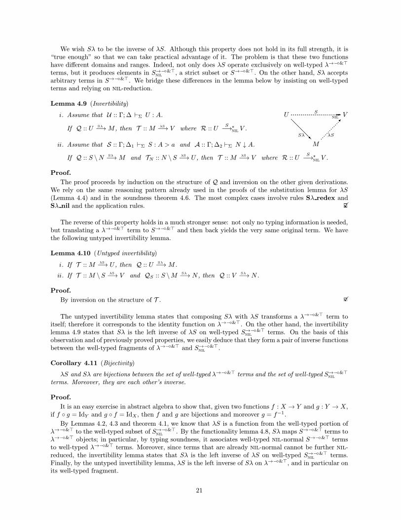
Lemma 4.9 (Invertibility)

i . Assume that U :: Γ; ∆ `Σ U : A.

If Q :: U Sλ−→M , then T :: M λS−→ V where R :: US−→∗

nilV .

U

M

V

@@@@RSλ ...

......

.....�

λS

.........................-S.........................-nil

-

ii . Assume that S :: Γ; ∆1 `Σ S : A > a and A :: Γ; ∆2 `Σ N ↓ A.

If Q :: S \N Sλ−→M and TN :: N \S λS−→ U , then T :: M λS−→ V where R :: US−→∗

nilV .

Proof.

The proof proceeds by induction on the structure of Q and inversion on the other given derivations.We rely on the same reasoning pattern already used in the proofs of the substitution lemma for λS(Lemma 4.4) and in the soundness theorem 4.6. The most complex cases involve rules Sλ redex andSλ nil and the application rules. 2X

The reverse of this property holds in a much stronger sense: not only no typing information is needed,but translating a λ→−◦&> term to S→−◦&> and then back yields the very same original term. We havethe following untyped invertibility lemma.

Lemma 4.10 (Untyped invertibility)

i . If T :: M λS−→ U , then Q :: U Sλ−→M .

ii . If T :: M \S λS−→ V and QS :: S \M Sλ−→ N , then Q :: V Sλ−→ N .

Proof.

By inversion on the structure of T . 2X

The untyped invertibility lemma states that composing Sλ with λS transforms a λ→−◦&> term toitself; therefore it corresponds to the identity function on λ→−◦&>. On the other hand, the invertibilitylemma 4.9 states that Sλ is the left inverse of λS on well-typed S→−◦&>

nilterms. On the basis of this

observation and of previously proved properties, we easily deduce that they form a pair of inverse functionsbetween the well-typed fragments of λ→−◦&> and S→−◦&>

nil.

Corollary 4.11 (Bijectivity)

λS and Sλ are bijections between the set of well-typed λ→−◦&> terms and the set of well-typed S→−◦&>nil

terms. Moreover, they are each other’s inverse.

Proof.

It is an easy exercise in abstract algebra to show that, given two functions f : X → Y and g : Y → X,if f ◦ g = IdY and g ◦ f = IdX , then f and g are bijections and moreover g = f−1.

By Lemmas 4.2, 4.3 and theorem 4.1, we know that λS is a function from the well-typed portion ofλ→−◦&> to the well-typed subset of S→−◦&>

nil. By the functionality lemma 4.8, Sλ maps S→−◦&> terms to

λ→−◦&> objects; in particular, by typing soundness, it associates well-typed nil-normal S→−◦&> termsto well-typed λ→−◦&> terms. Moreover, since terms that are already nil-normal cannot be further nil-reduced, the invertibility lemma states that Sλ is the left inverse of λS on well-typed S→−◦&>

nilterms.

Finally, by the untyped invertibility lemma, λS is the left inverse of Sλ on λ→−◦&>, and in particular onits well-typed fragment.

21

S→−◦&> λ→−◦&>

Sλ

Figure 8: Sλ

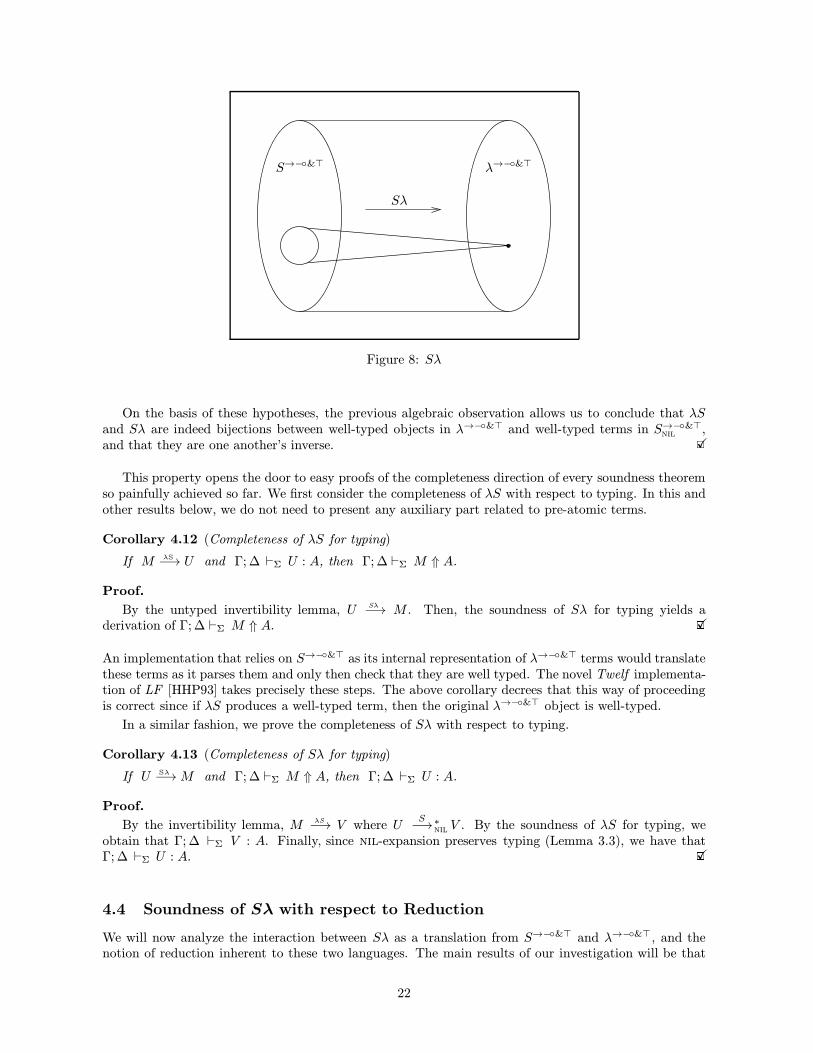
On the basis of these hypotheses, the previous algebraic observation allows us to conclude that λSand Sλ are indeed bijections between well-typed objects in λ→−◦&> and well-typed terms in S→−◦&>

nil,

and that they are one another’s inverse. 2X

This property opens the door to easy proofs of the completeness direction of every soundness theoremso painfully achieved so far. We first consider the completeness of λS with respect to typing. In this andother results below, we do not need to present any auxiliary part related to pre-atomic terms.

Corollary 4.12 (Completeness of λS for typing)

If M λS−→ U and Γ; ∆ `Σ U : A, then Γ; ∆ `Σ M ⇑ A.

Proof.

By the untyped invertibility lemma, U Sλ−→ M . Then, the soundness of Sλ for typing yields aderivation of Γ; ∆ `Σ M ⇑ A. 2X

An implementation that relies on S→−◦&> as its internal representation of λ→−◦&> terms would translatethese terms as it parses them and only then check that they are well typed. The novel Twelf implementa-tion of LF [HHP93] takes precisely these steps. The above corollary decrees that this way of proceedingis correct since if λS produces a well-typed term, then the original λ→−◦&> object is well-typed.

In a similar fashion, we prove the completeness of Sλ with respect to typing.

Corollary 4.13 (Completeness of Sλ for typing)

If U Sλ−→M and Γ; ∆ `Σ M ⇑ A, then Γ; ∆ `Σ U : A.

Proof.

By the invertibility lemma, M λS−→ V where US−→∗

nilV . By the soundness of λS for typing, we

obtain that Γ; ∆ `Σ V : A. Finally, since nil-expansion preserves typing (Lemma 3.3), we have thatΓ; ∆ `Σ U : A. 2X

4.4 Soundness of Sλ with respect to Reduction

We will now analyze the interaction between Sλ as a translation from S→−◦&> and λ→−◦&>, and thenotion of reduction inherent to these two languages. The main results of our investigation will be that

22

Sλ preserves β-reductions, but identifies nil-convertible terms. We will also take advantage of the factthat this translation is the inverse of λS to prove the completeness counterpart of these statements.

It will be convenient to start by getting a deeper understanding of how nil-reducibility relates to Sλ.

Consider the equivalence relationS≡nil induced by the nil-reduction congruence

S−→nil. Its equivalenceclasses consist of all the terms of S→−◦&> that nil-reduce to the same nil-normal form. Sλ uniformlymaps every object in such an equivalence class to the same λ→−◦&> term, as depicted in Figure 8. Inorder to prove this fact, we first show that nil-reducing a term does not affect its translation.

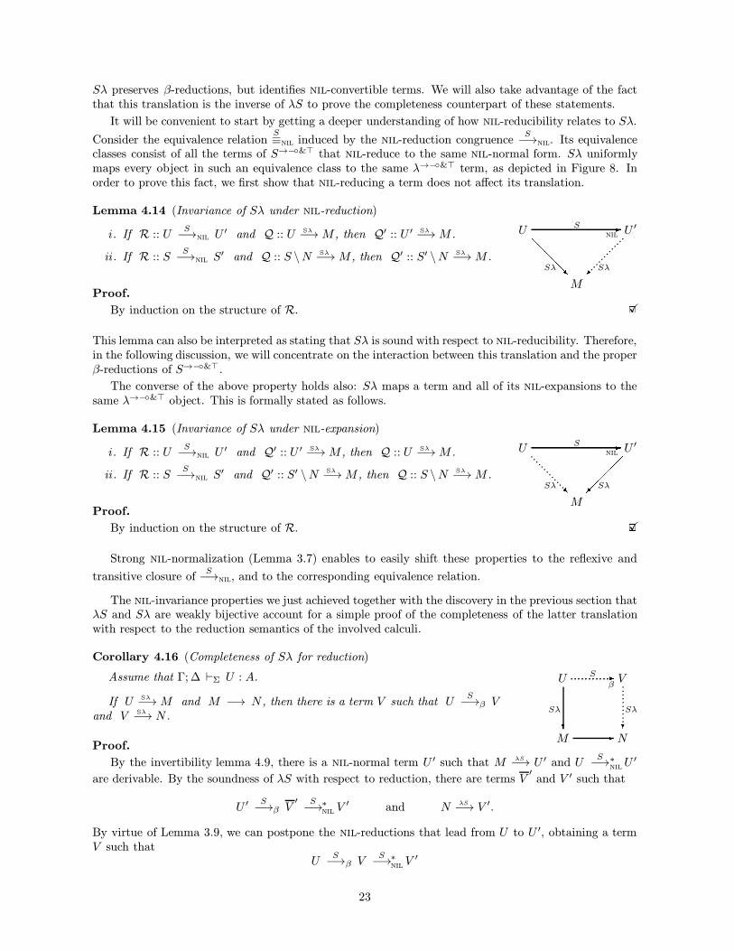
Lemma 4.14 (Invariance of Sλ under nil-reduction)

i . If R :: US−→nil U

′ and Q :: U Sλ−→M , then Q′ :: U ′ Sλ−→M .

ii . If R :: SS−→nil S

′ and Q :: S \N Sλ−→M , then Q′ :: S′ \N Sλ−→M .

U

M

U ′

@@@@RSλ

-S -nil ..............Sλ

Proof.

By induction on the structure of R. 2X

This lemma can also be interpreted as stating that Sλ is sound with respect to nil-reducibility. Therefore,in the following discussion, we will concentrate on the interaction between this translation and the properβ-reductions of S→−◦&>.

The converse of the above property holds also: Sλ maps a term and all of its nil-expansions to thesame λ→−◦&> object. This is formally stated as follows.

Lemma 4.15 (Invariance of Sλ under nil-expansion)

i . If R :: US−→nil U

′ and Q′ :: U ′ Sλ−→M , then Q :: U Sλ−→M .

ii . If R :: SS−→nil S

′ and Q′ :: S′ \N Sλ−→M , then Q :: S \N Sλ−→M .

U

M

U ′

����Sλ

-S -nil..............RSλ

Proof.

By induction on the structure of R. 2X

Strong nil-normalization (Lemma 3.7) enables to easily shift these properties to the reflexive and

transitive closure ofS−→nil, and to the corresponding equivalence relation.

The nil-invariance properties we just achieved together with the discovery in the previous section thatλS and Sλ are weakly bijective account for a simple proof of the completeness of the latter translationwith respect to the reduction semantics of the involved calculi.

Corollary 4.16 (Completeness of Sλ for reduction)

Assume that Γ; ∆ `Σ U : A.

If U Sλ−→M and M −→ N , then there is a term V such that US−→β V

and V Sλ−→ N .

U

M

V

N?

Sλ

-

...........?Sλ

............-S............-β

Proof.

By the invertibility lemma 4.9, there is a nil-normal term U ′ such that M λS−→ U ′ and US−→∗

nilU ′

are derivable. By the soundness of λS with respect to reduction, there are terms V′

and V ′ such that

U ′S−→β V

′ S−→∗nilV ′ and N λS−→ V ′.

By virtue of Lemma 3.9, we can postpone the nil-reductions that lead from U to U ′, obtaining a termV such that

US−→β V

S−→∗nilV ′

23

On the other hand, by untyped invertibility, there is a derivation of V ′ Sλ−→ N . At this point, an iterateduse of the invariance of Sλ under nil-expansion (Lemma 4.15) allows us to obtain the desired derivationof V Sλ−→ N . 2X

We conclude this section by showing that Sλ is sound with respect to the reduction semantics ofS→−◦&>. The above invariance lemmas capture this property in the case of nil-reduction. Therefore, wefocus the discussion on β-reductions.

The required steps in order to achieve this result are reminiscent of the path we followed when provingthe analogous statement for λS. There are however three important differences. First, the proofs aremuch simpler in the present case. Second, the statements below do not need to mention any typinginformation. Third, nil-reductions do not appear in these statements. This overall simplification derivesfrom the fact that, because of the presence of nil-reduction, S→−◦&> has more structure than λ→−◦&>.Therefore, while λS needed to extract the additional information from a typing derivation, Sλ can simplyforget about the extra structure of the S→−◦&> terms it acts upon.

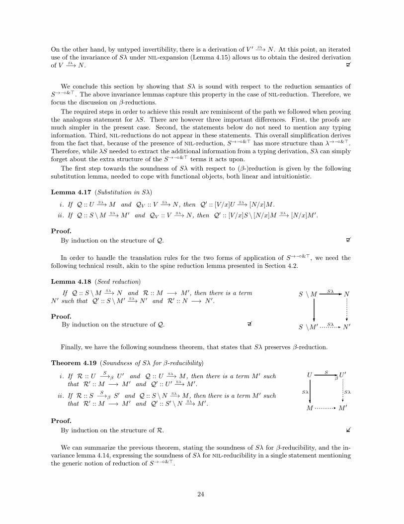
The first step towards the soundness of Sλ with respect to (β-)reduction is given by the followingsubstitution lemma, needed to cope with functional objects, both linear and intuitionistic.

Lemma 4.17 (Substitution in Sλ)

i . If Q :: U Sλ−→M and QV :: V Sλ−→ N , then Q′ :: [V/x]U Sλ−→ [N/x]M .

ii . If Q :: S \M Sλ−→M ′ and QV :: V Sλ−→ N , then Q′ :: [V/x]S \ [N/x]M Sλ−→ [N/x]M ′.

Proof.

By induction on the structure of Q. 2X

In order to handle the translation rules for the two forms of application of S→−◦&>, we need thefollowing technical result, akin to the spine reduction lemma presented in Section 4.2.

Lemma 4.18 (Seed reduction)

If Q :: S \M Sλ−→ N and R :: M −→ M ′, then there is a termN ′ such that Q′ :: S \M ′ Sλ−→ N ′ and R′ :: N −→ N ′.

Proof.By induction on the structure of Q. 2X

S \M N

S \M ′ N ′

-Sλ

?..........-Sλ

...........?

Finally, we have the following soundness theorem, that states that Sλ preserves β-reduction.

Theorem 4.19 (Soundness of Sλ for β-reducibility)

i . If R :: US−→β U ′ and Q :: U Sλ−→ M , then there is a term M ′ such

that R′ :: M −→ M ′ and Q′ :: U ′ Sλ−→M ′.

ii . If R :: SS−→β S′ and Q :: S \N Sλ−→M , then there is a term M ′ such

that R′ :: M −→ M ′ and Q′ :: S′ \N Sλ−→M ′.

U U ′

M M ′

-S -β

?Sλ

..........-

...........?Sλ

Proof.

By induction on the structure of R. 2X

We can summarize the previous theorem, stating the soundness of Sλ for β-reducibility, and the in-variance lemma 4.14, expressing the soundness of Sλ for nil-reducibility in a single statement mentioningthe generic notion of reduction of S→−◦&>.

24

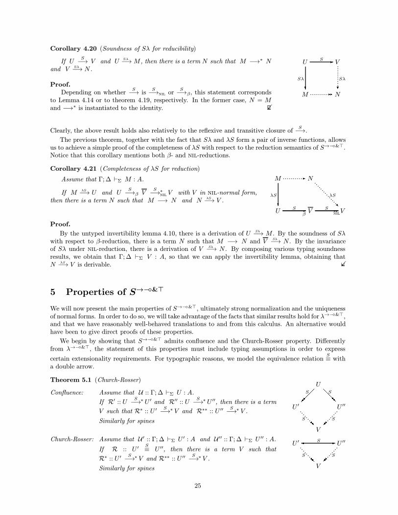
Corollary 4.20 (Soundness of Sλ for reducibility)

If US−→ V and U Sλ−→M , then there is a term N such that M −→∗ N

and V Sλ−→ N .

Proof.Depending on whether

S−→ isS−→nil or

S−→β, this statement correspondsto Lemma 4.14 or to theorem 4.19, respectively. In the former case, N = Mand −→∗ is instantiated to the identity. 2X

U V

M N

-S

?Sλ

...........--

...........?Sλ

Clearly, the above result holds also relatively to the reflexive and transitive closure ofS−→.

The previous theorem, together with the fact that Sλ and λS form a pair of inverse functions, allowsus to achieve a simple proof of the completeness of λS with respect to the reduction semantics of S→−◦&>.Notice that this corollary mentions both β- and nil-reductions.

Corollary 4.21 (Completeness of λS for reduction)

Assume that Γ; ∆ `Σ M : A.

If M λS−→ U and US−→β V

S−→∗nilV with V in nil-normal form,

then there is a term N such that M −→ N and N λS−→ V .

M

U

N

V V?

λS

-S -β

-S -nil

-

...........-................R

λS

Proof.

By the untyped invertibility lemma 4.10, there is a derivation of U Sλ−→ M . By the soundness of Sλwith respect to β-reduction, there is a term N such that M −→ N and V Sλ−→ N . By the invarianceof Sλ under nil-reduction, there is a derivation of V Sλ−→ N . By composing various typing soundnessresults, we obtain that Γ; ∆ `Σ V : A, so that we can apply the invertibility lemma, obtaining thatN λS−→ V is derivable. 2X

5 Properties of S→−◦&>

We will now present the main properties of S→−◦&>, ultimately strong normalization and the uniquenessof normal forms. In order to do so, we will take advantage of the facts that similar results hold for λ→−◦&>,and that we have reasonably well-behaved translations to and from this calculus. An alternative wouldhave been to give direct proofs of these properties.

We begin by showing that S→−◦&> admits confluence and the Church-Rosser property. Differentlyfrom λ→−◦&>, the statement of this properties must include typing assumptions in order to express

certain extensionality requirements. For typographic reasons, we model the equivalence relationS≡ with

a double arrow.

Theorem 5.1 (Church-Rosser)

Confluence: Assume that U :: Γ; ∆ `Σ U : A.

If R′ :: US−→∗ U ′ and R′′ :: U

S−→∗ U ′′, then there is a term

V such that R∗ :: U ′S−→∗ V and R∗∗ :: U ′′

S−→∗ V .

Similarly for spines

U

U ′ U ′′

V

@@RS

R��S

.........S

.........RSR

Church-Rosser: Assume that U ′ :: Γ; ∆ `Σ U ′ : A and U ′′ :: Γ; ∆ `Σ U ′′ : A.

If R :: U ′S≡ U ′′, then there is a term V such that

R∗ :: U ′S−→∗ V and R∗∗ :: U ′′

S−→∗ V .

Similarly for spines

U ′ U ′′

V

-S�.........

S

.........RSR

25

Proof.

We will carry out the proof in the case of confluence only. The Church-Rosser property is handledsimilarly.

Since, by Lemma 4.8, Sλ is a total function over S→−◦&>, there is a unique term M such thatU Sλ−→M is derivable. By typing soundness, we obtain that Γ; ∆ `Σ M ⇑ A. By iterated applications ofthe soundness of Sλ over reduction, we deduce that there are terms M ′ and M ′′ such that M −→∗ M ′and U ′ Sλ−→ M ′, and similarly M −→∗ M ′′ and U ′′ Sλ−→ M ′′. By subject reduction, we have thatΓ; ∆ `Σ M ′ ⇑ A and Γ; ∆ `Σ M ′′ ⇑ A. By the confluence property of λ→−◦&>, we know that thereexists a term N such that M ′ −→∗ N and M ′′ −→∗ N are derivable.

By the invertibility lemma, there are S→−◦&> terms U∗ and U∗∗ such thatM ′ λS−→ U∗ with U ′S−→∗

nilU∗

and M ′′ λS−→ U∗∗ with U ′′S−→∗

nilU∗∗. By the soundness of λS with respect to reductions, there are terms

V ′ and V ′′ such that U∗S−→∗ V ′ and N λS−→ V ′, and similarly U∗∗

S−→∗ V ′′ and N λS−→ V ′′. However,since λS is a function, V ′ = V ′′; let us call this term V . By composing the various reductions above, we

obtain the desired derivations of U ′S−→∗ V and U ′′

S−→∗ V . 2X

Next, we consider the S→−◦&> equivalent of the transitivity lemma 2.3 discussed in Section 2. As inλ→−◦&>, we must distinguish the linear and the intuitionistic cases, but we have no convenient notationthat spans uniformly over terms and spines. Therefore, the lemma below has four parts.

Lemma 5.2 (Transitivity)

i . If U :: Γ; ∆, x :B `Σ U : A and UV :: Γ; ∆′ `Σ V : B, then U ′ :: Γ; ∆,∆′ `Σ [V/x]U : A.

ii . If S :: Γ; ∆, x :B `Σ S : A > a and UV :: Γ; ∆′ `Σ V : B, then S′ :: Γ; ∆,∆′ `Σ [V/x]S : A > a.

iii . If U :: Γ, x :B; ∆ `Σ U : A and UV :: Γ; · `Σ V : B, then U ′ :: Γ; ∆ `Σ [V/x]U : A.

iv. If S :: Γ, x :B; ∆ `Σ S : A > a and UV :: Γ; · `Σ V : B, then U ′ :: Γ; ∆ `Σ [V/x]S : A > a.

Proof.

We prove this lemma by means of a technique similar to the one we just sketched in the case of theChurch-Rosser property. We illustrate the manner spines are handled by presenting the full treatment ofcase (ii). The treatment of the other parts is similar or simpler.

Let z be a variable that does not appear in neither Γ, ∆, nor ∆′, and that is different from x. We willuse it as a generic head for S. By rule lλ lvar, there is a (trivial) typing derivation of Γ; z :A `Σ z ↓ A.On the basis of this fact, by the soundness of Sλ for typing (Theorem 4.7), there is a term M suchthat S \ z Sλ−→ M and Γ; ∆, x : B, z : A `Σ M ⇑ a are derivable. By the same theorem, there is aterm N and derivations of V Sλ−→ N and Γ; ∆′ `Σ N ⇑ B. By the transitivity lemma 2.3 for λ→−◦&>,Γ; ∆,∆′, z :A `Σ [N/x]M ⇑ a is derivable.

By rule λS var, there is a derivation of z \S λS−→ z ·S. By the invertibility lemma 4.9, there is a term

U ′ and derivations of M λS−→ U ′ and z · S S−→∗nilU ′. By inversion on the reduction rules for S→−◦&>,

U ′ = z · S′ for some spine S′. Therefore, by rule Sr var, there must be a derivation of SS−→∗

nilS′.

Again by the invertibility lemma 4.9, there is a term V ′ and a derivation N λS−→ V ′, where VS−→∗

nilV ′

is derivable. By the substitution lemma 4.4, there is a term V and derivations of [N/x]M λS−→ V and

z · ([V ′/x]S′)S−→∗

nilV (remember that x 6= z). Again by invertibility on the reduction rules for S→−◦&>,

V = z ·S for some spine S, and [V ′/x]S′S−→∗

nilS. By iterated applications of the substitution lemma 3.8,

there is a derivation of [V/x]SS−→∗

nilS.

By the soundness of λS with respect to typing, Γ; ∆,∆′, z :A `Σ z · S : a is derivable. By inversionon rule lS lvar, Γ; ∆,∆′ `Σ S : A > a is derivable as well. Now, since nil-expansion preserves typing,there is a derivation of Γ; ∆,∆′ `Σ [V/x]S : A > a. 2X

The next property we are interested in proving for S→−◦&> is subject reduction. Again, we mustdeal separately with terms and with spines. Remember that we have already proved this property in thesubcase of nil-reduction.

26

Lemma 5.3 (Subject reduction)

i . If U :: Γ; ∆ `Σ U : A and Q :: US−→ V , then U ′ :: Γ; ∆ `Σ V : A.

ii . If S :: Γ; ∆ `Σ S : A > a and Q :: SS−→ S′, then S′ :: Γ; ∆ `Σ S′ : A > a.

Proof.

We will prove only part (i) of this statement. Part (ii) adapts the technique we just applied in thetransitivity lemma.

By the soundness of Sλ with respect to typing, there are a term M and derivations of U Sλ−→M andΓ; ∆ `Σ M ⇑ A. By the soundness of Sλ with respect to reductions, there are a term N and derivationsof V Sλ−→ N and M −→∗ N . By the subject reduction property of λ→−◦&>, Γ; ∆ `Σ N ⇑ A is derivable.

Now, by the soundness of λS with respect to typing, there is a term V ′ such that Γ; ∆ `Σ V ′ : A andN λS−→ V ′ are derivable. On the other hand, by the invertibility lemma 4.9, there is a term V ′′ such that

N λS−→ V ′′ and VS−→∗

nilV ′′ are derivable. However, since, by Lemma 4.2, λS is a function, we have that

V ′ = V ′′. Then, in order to conclude this proof, we simply take advantage of the fact that nil-expansionpreserves typing (Lemma 3.3) to obtain the desired derivation of Γ; ∆ `Σ V : A. 2X

We now tackle strong normalization which, as in the case of λ→−◦&>, states that no infinite chainof (either nil- or β-) reductions can start from a well-typed S→−◦&> term. Therefore, we can reduce awell-typed term to normal (actually canonical) form by exhaustively reducing randomly selected redices.

Theorem 5.4 (Strong normalization)

i . If U :: Γ; ∆ `Σ U : A, then U is strongly normalizing.

ii . If S :: Γ; ∆ `Σ S : A > a, then S is strongly normalizing.

Proof.

We will prove only part (i) of this theorem. Part (ii) is handled similarly.

Assume we have a (possibly infinite) sequence of terms U0, U1, U2, . . . such that U = U0 and there arederivations for the following reductions:

σ = U0S−→ U1

S−→ U2S−→ . . .

By the soundness of Sλ with respect to reducibility, every β-reduction in σ corresponds to a reduction inλ→−◦&> (Theorems 4.19) while every nil-reduction disappears (Lemma 4.14). This entails that there is asequence of λ→−◦&> term M0,M1,M2, . . . such that on the one hand there are derivations of Ui

Sλ−→Mϕ(i)

where ϕ maps maximal subsequences of σ linked by nil-reductions to the same λ→−◦&> term, and onthe other hand the following reduction sequence is derivable

σ′ = M0 −→ M1 −→ M2 −→ . . .

Notice in particular that there is a derivation of U Sλ−→ M0. Therefore, by the soundness of Sλ withrespect to typing, the judgment Γ; ∆ `Σ M0 ⇑ A is derivable. By the strong normalization theoremfor λ→−◦&>, σ′ is finite. Then, also σ must be finite since, by the strong normalization of nil-reduction(Lemma 3.7), the maximal subsequences of nil-reducts collapsed by ϕ are finite. 2X

Strong normalization ensures that exhaustive reductions of a well-typed S→−◦&> term (or spine) willeventually produce an object in normal form. Depending on which redex is selected at each step, thisprocedure might yield different normal objects. The uniqueness corollary below guarantees that everyreduction path will lead to the same normal term (or spine), up to the renaming of bound variables.

Corollary 5.5 (Uniqueness of normal forms)

i . If U :: Γ; ∆ `Σ U : A, then there is a unique normal term V such that Q′ :: U −→∗ V .

27

ii . If S :: Γ; ∆ `Σ S : A > a, then there is a unique normal spine S′ such that Q′ :: S −→∗ S′.

Proof.

By the strong normalization theorem, we know that every sequence of reductions starting at U leadsto a term in normal form. Let consider two reduction sequences validating U −→∗ V ′ and U −→∗ V ′′,for terms V ′ and V ′′ in normal form. By confluence, there is a term V to which both reduce. However,since V ′ and V ′′ do not contain redices, the only way to close the diamond is to have that V ′ = V ′′ = V ,and use the identical reduction.

We proceed similarly in order to prove the second part of this statement. 2X

As in the case of λ→−◦&>, the above results entitle speaking about the normal form (or equivalentlythe canonical form) of a term U or a spine S, whenever these objects are well-typed. We denote thisterm and spine Can(U) and Can(S), respectively. A calculus that accepts only canonical objects can beobtained from the typing system displayed in Figure 3 by simply removing rule lS redex.

A term (spine) in which redices appear at most in the argument of an application is said to be inweak head-normal form. Any well-typed term can be converted to weak-head normal form by repeatedlyselecting a redex that violates this property and reducing it. A similar property holds for spines. Weuse U and S to denote the weak-head normal form of a term U and a spine S, respectively. Weakhead-normalization is not as computationally expensive as full normalization since it operates on shallowredices only. However, it exposes enough of a normal form to work comfortably in many circumstances.Therefore, the implementation of procedures that, by their very nature, need to perform reductions,unification for example, often rely on weak head-normalization rather than on full normalization.

6 Further Remarks

In this section, we briefly report on important relationships between our spine calculus and other formalsystems in the literature. More precisely, we hint at an alternative development of the results obtainedin this paper (Section 6.1), point at a relationship between the spine calculus and the logic programmingnotion of uniform derivability (Section 6.2), and discuss related work (Section 6.3).

6.1 Alternative Development

We observed that the spine calculus S→−◦&> has more structure than the corresponding traditionalformulation, as manifested by the presence of the nil-reduction rule, which has no equivalent in λ→−◦&>.When analyzing the translation function λS, we had to recover this additional structure by accompanyingmost statements with λ→−◦&> typing derivations. This step was over-restrictive, but acceptable becauseof our interest in well-typed terms only.

We can achieve a better correspondence by enriching the syntax of λ→−◦&> with the two new operatorsac and ca. Let us call the enriched language λ→−◦&>ac . We use these new constructs to annotate thecoercion rules lλ atm and lλ redex, which become:

Γ; ∆ `Σ M ↓ alλ atm

Γ; ∆ `Σ acM ⇑ aΓ; ∆ `Σ M ⇑ A

lλ redex

Γ; ∆ `Σ caM ↓ A

Notice that every typing derivation Γ; ∆ `Σ M ⇑↓ A can now be uniquely reconstructed on the basisof the term M , except for the composition of the context Γ; ∆ (in particular, the manner ∆ is split incertain applications of multiplicative rules).

We augment the reduction semantics of λ→−◦&> with the rule

βac : ca (acM) −→ M

which corresponds to eliminating alternations of rules lλ atm and lλ redex. We call the expression on

28

the left-hand side of the arrow a coercion redex. The other reduction rules are upgraded as follows:

fst (ca 〈M,N〉) −→ Msnd (ca 〈M,N〉) −→ N

(ca (λx :A.M))ˆN −→ [N/x]M(ca (λx :A.M))N −→ [N/x]M

Then, the absence of any occurrence of ca in a well-typed term implies that a term does not containredices, and therefore that it is in normal form.

We modify the translation rules λS atm and λS redex as follows:

M \nilλS−→ H · S

λS atm

acM λS−→ H · SM λS−→ U

λS redex

caM \S λS−→ U · S

Notice the absence of side-conditions. On the basis of these upgraded definitions, it is easy to see thatλS maps coercion redices to nil redices, and therefore applications of the new reduction rule βac areemulated in S→−◦&> by nil-reductions.

Rules Sλ con, Sλ var and Sλ redex of Sλ are modified as follows:

S \ c Sλ−→MSλ con

c · S Sλ−→ acM

S \ x Sλ−→MSλ var

x · S Sλ−→ acM

U Sλ−→M ′ S \caM ′ Sλ−→MSλ redex

U · S Sλ−→ acM

The new and improved Sλ translates nil-redices to coercion redices and puts nil-reductions and βac inone-to-one correspondence. As we suggested, this treatment eliminates the mismatch between λ→−◦&>

and S→−◦&> that led to many of the complications in Section 4.

Using λ→−◦&>ac as an external language is impractical for most applications. Indeed, a more reasonableapproach is to give the user the simpler λ→−◦&> and have coercions filled in during parsing; this isessentially what λS did in the previous sections. Coercions need to be inserted at every alternation ofconstructors and destructors in a term. Notice that the resulting object does not contain coercion redicesbut, similarly to nil-redices, they may be exposed by the application of β-reductions. Further flexibilitycan be achieved by relieving the user from the requirement of writing terms in η-long form only: subtermscan be expanded as soon as their type has been inferred as a result of type checking.

6.2 Relationship to Uniform Provability

An abstract logic programming language [MNPS91] is a fragment of a logic such that every derivable se-quent has a uniform derivation. An intuitionistic cut-free sequent derivation is uniform if it is constructedin the following way, from the bottom up: right introduction rules are applied until the formula on theright-hand side of the sequent (the goal formula) is atomic, then a formula on the left-hand side (theprogram) of the sequent is selected (the focus or stoup) and left introduction rules are applied to it untilthe same atomic formula is exposed, possibly spawning subgoals that are to have uniform proofs.

The fragment of linear logic obtained by considering the types of λ→−◦&> and S→−◦&> as logicformulas is known as the language of (propositional) linear hereditary Harrop formulas [HM94, Cer96].We denoted it ILL→−◦&> in Section 2. This formalism is an abstract logic programming language anda uniform proof system for it, adapted from [Cer96], is reported in Figure 9. The uniform provabilityjudgment

Γ; ∆u−→ A

is subject to the application of the right introduction rules of a sequent calculus presentation of ILL→−◦&>.When an atomic formula a is exposed (rules u lin and u int), a program formulaA is selected and isolatedin the central part of the immediate entailment judgment

Γ; ∆u−→ A � a

and left introduction rules are applied to it.

29

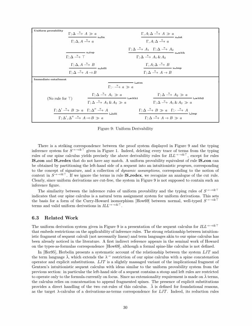
Uniform provability

Γ; ∆u−→ A � a

u lin

Γ; ∆, Au−→ a

Γ, A; ∆u−→ A � a

u int

Γ, A; ∆u−→ a

u top

Γ; ∆u−→ >

Γ; ∆u−→ A1 Γ; ∆

u−→ A2u with

Γ; ∆u−→ A1 &A2

Γ; ∆, Au−→ B

u lolli

Γ; ∆u−→ A−◦B

Γ, A; ∆u−→ B

u imp

Γ; ∆u−→ A→ B

Immediate entailment

i atm

Γ; · u−→ a � a

(No rule for >)Γ; ∆

u−→ A1 � ai with1

Γ; ∆u−→ A1 &A2 � a

Γ; ∆u−→ A2 � a

i with2

Γ; ∆u−→ A1 &A2 � a

Γ; ∆′u−→ B � a Γ; ∆′′

u−→ Ai lolli

Γ; ∆′,∆′′u−→ A−◦B � a

Γ; ∆u−→ B � a Γ; · u−→ A

i imp

Γ; ∆u−→ A→ B � a

Figure 9: Uniform Derivability

There is a striking correspondence between the proof system displayed in Figure 9 and the typinginference system for S→−◦&> given in Figure 1. Indeed, deleting every trace of terms from the typingrules of our spine calculus yields precisely the above derivability rules for ILL→−◦&>, except for ruleslS con and lS redex that do not have any match. A uniform provability equivalent of rule lS con canbe obtained by partitioning the left-hand side of a sequent into an intuitionistic program, correspondingto the concept of signature, and a collection of dynamic assumptions, corresponding to the notion ofcontext in S→−◦&>. If we ignore the terms in rule lS redex, we recognize an analogue of the cut rule.Clearly, since uniform derivations are cut-free, the system in Figure 9 is not supposed to contain such aninference figure.

The similarity between the inference rules of uniform provability and the typing rules of S→−◦&>

indicates that our spine calculus is a natural term assignment system for uniform derivations. This setsthe basis for a form of the Curry-Howard isomorphism [How69] between normal, well-typed S→−◦&>

terms and valid uniform derivations in ILL→−◦&>.

6.3 Related Work

The uniform derivation system given in Figure 9 is a presentation of the sequent calculus for ILL→−◦&>

that embeds restrictions on the applicability of inference rules. The strong relationship between intuition-istic fragment of sequent calculi (not necessarily linear) and term languages akin to our spine calculus hasbeen already noticed in the literature. A first indirect reference appears in the seminal work of Howardon the types-as-formulas correspondence [How69], although a formal spine-like calculus is not defined.

In [Her95], Herbelin presents a systematic account of the relationship between the system LJT andthe term language λ, which extends the λ→ restriction of our spine calculus with a spine concatenationoperator and explicit substitutions. LJT is a slightly massaged variant of the implicational fragment ofGentzen’s intuitionistic sequent calculus with ideas similar to the uniform provability system from theprevious section: in particular the left-hand side of a sequent contains a stoup and left rules are restrictedto operate only to the formula currently on focus. Since no extensionality requirement is made on λ terms,the calculus relies on concatenation to append fragmented spines. The presence of explicit substitutionsprovides a direct handling of the two cut-rules of this calculus. λ is defined for foundational reasons,as the target λ-calculus of a derivations-as-terms correspondence for LJT . Indeed, its reduction rules

30

correspond to the steps in a cut-elimination procedure for LJT, so that strong normalization theorem forλ subsumes the cut-elimination property for this logic.

Schwichtenberg [Sch97] adopts a similar approach relatively to a richer logic consisting of implication,conjunction and universal quantification. He starts from a more traditional presentation of the sequentcalculus. In particular the absence of a stoup forces him to consider permutative conversions. Theterm calculus he proposes differs from Herbelin’s by the absence of explicit concatenation operators andsubstitutions. It is therefore more similar to our spine calculus.

Barendregt [Bar80] relies on an term language akin to our spine calculus to study the notion ofnormalization in the untyped λ-calculus. Terms in this language are called Bohm trees.

7 Conclusion and Future Work

In this paper, we have formalized an alternative presentation of the linear λ-calculus λ→−◦&> which we be-lieve can be used to improve the efficiency of critical procedures such as unification in the implementationof languages based on (linear) λ-calculi. The resulting language, the spine calculus S→−◦&>, strengthensthe natural adaptation of the notion of abstract Bohm tree [Bar80, Her95] to encompass extensionalproducts (&), a unit type (>) and linearity (−◦), with the further requirement that well-typed terms bein η-long form. S→−◦&> terms of base type are structured similarly to the objects found in first-orderterm languages. In particular, their head is immediately available, an important benefit for proceduressuch as unification that base a number of choices on the nature of the heads of the terms they operateupon. Having extensionality built-in permits avoiding the overhead, both in terms of bookkeeping andexecution time, of performing η-conversions at run time.

The intended applications of this work lie in proof search, logic programming, and the implementationof logical frameworks based on linear type theories. In particular, the spine calculus S→−◦&> has beendesigned as a first approximation of an internal representation for the type theory λΠ−◦&> underlying thelinear logical framework LLF [Cer96, CP96]. An extension to the full language, which includes dependenttypes, does not appear to be problematic. The adoption of a spine calculus as an internal representationdevice appears to integrate well with the simultaneous use of explicit substitutions [ACCL91]. However,the details of the amalgamation of these two techniques in the presence of linearity still need to be workedout.

A variant of the spine calculus deprived of linear constructs, but featuring dependent types andexplicit substitutions is currently tested in a new implementation of the linear framework LF [HHP93] asa higher-order constraint logic programming language. This system, called Twelf, is expected to supersedethe Elf implementation of LF currently in use [Pfe91, Pfe94]. It will be available later this year.

Acknowledgments

We would like to thank Carsten Schurmann for the insight he provided as a co-implementor of Twelf andthrough numerous discussions. We are also deeply indebted to Helmut Schwichtenberg for the fruitfuldiscussions and for pointing out literature relevant to the topics treated in this paper.

References

[ACCL91] Martın Abadi, Luca Cardelli, Pierre-Louis Curien, and Jean-Jacques Levy. Explicit substitutions.Journal of Functional Programming, 1(4):375–416, October 1991.

[Bar80] H. P. Barendregt. The Lambda-Calculus: Its Syntax and Semantics. North-Holland, 1980.

[Bar96] Andrew Barber. Dual intuitionistic linear logic. Technical Report ECS-LFCS-96-347, Laboratory forFoundations of Computer Sciences, University if Edinburgh, 1996.

[Cer96] Iliano Cervesato. A Linear Logical Framework. PhD thesis, Dipartimento di Informatica, Universitadi Torino, February 1996.

[Chu40] Alonzo Church. A formulation of a simple theory of types. Journal of Symbolic Logic, 5:56–68, 1940.

31

[CP96] Iliano Cervesato and Frank Pfenning. A linear logical framework. In E. Clarke, editor, Proceedings ofthe Eleventh Annual Symposium on Logic in Computer Science, pages 264–275, New Brunswick, NewJersey, July 1996. IEEE Computer Society Press.

[CP97] Iliano Cervesato and Frank Pfenning. Linear higher-order pre-unification. Technical report, Depart-ment of Computer Science, Carnegie Mellon University, 1997. Forthcoming.

[dB72] N. G. de Bruijn. Lambda-calculus notation with nameless dummies: a tool for automatic formulamanipulation with application to the Church-Rosser theorem. Indag. Math., 34(5):381–392, 1972.

[DJ90] Nachum Dershowitz and Jean-Pierre Jouannaud. Handbook of Theoretical Computer Science, vol-ume B, chapter Rewrite Systems, pages 243–320. MIT Press, 1990.

[Gir87] Jean-Yves Girard. Linear logic. Theoretical Computer Science, 50:1–102, 1987.

[Her95] Hugo Herbelin. A λ-calculus structure isomorphic to Genzten-style sequent calculus structure. InL. Pacholski and J. Tiuryn, editors, Computer Science Logic, Eighth Workshop — CSL’94, pages61–75, Kazimierz, Poland, 1995. Springer Verlag LNCS 933.

[HHP93] Robert Harper, Furio Honsell, and Gordon Plotkin. A framework for defining logics. Journal of theAssociation for Computing Machinery, 40(1):143–184, January 1993.

[HM94] Joshua Hodas and Dale Miller. Logic programming in a fragment of intuitionistic linear logic. Infor-mation and Computation, 110(2):327–365, 1994. A preliminary version appeared in the Proceedingsof the Sixth Annual IEEE Symposium on Logic in Computer Science, pages 32–42, Amsterdam, TheNetherlands, July 1991.

[How69] W. A. Howard. The formulae-as-types notion of construction. Unpublished manuscript, 1969.Reprinted in To H. B. Curry: Essays on Combinatory Logic, Lambda Calculus and Formalism, 1980.

[IP96] Samin Ishtiaq and David Pym. A relevant analysis of natural deduction, December 1996. Manuscript.

[JG95] C. Barry Jay and Neil Ghani. The virtues of eta-expansion. Journal of Functional Programming,2(5):135–154, 1995.

[Mil94] Dale Miller. A multiple-conclusion meta-logic. In S. Abramsky, editor, Ninth Annual IEEE Symposiumon Logic in Computer Science, pages 272–281, Paris, France, July 1994.

[MNPS91] Dale Miller, Gopalan Nadathur, Frank Pfenning, and Andre Scedrov. Uniform proofs as a foundationfor logic programming. Annals of Pure and Applied Logic, 51:125–157, 1991.

[MP92] Spiro Michaylov and Frank Pfenning. An empirical study of the runtime behavior of higher-orderlogic programs. In D. Miller, editor, Proceedings of the Workshop on the λProlog Programming Lan-guage, pages 257–271, Philadelphia, Pennsylvania, July 1992. University of Pennsylvania. Availableas Technical Report MS-CIS-92-86.

[NM88] Gopalan Nadathur and Dale Miller. An overview of λProlog. In Kenneth A. Bowen and Robert A.Kowalski, editors, Fifth International Logic Programming Conference, pages 810–827, Seattle, Wash-ington, August 1988. MIT Press.

[Pfe91] Frank Pfenning. Logic programming in the LF logical framework. In Gerard Huet and Gordon Plotkin,editors, Logical Frameworks, pages 149–181. Cambridge University Press, 1991.

[Pfe94] Frank Pfenning. Elf: A meta-language for deductive systems. In A. Bundy, editor, Proceedings of the12th International Conference on Automated Deduction, pages 811–815, Nancy, France, June 1994.Springer-Verlag LNAI 814. System abstract.

[Sch97] Helmut Schwichtenberg. Termination of permutative conversions in intuitionistic Gentzen calculi.Manuscript, March 1997.

32