A lecture on the representation theory of

partial Brauer algebras ∗

Paul Martin† (joint work with Volodymyr Mazorchuk‡)

Abstract

We construct the Specht modules and determine the corresponding de-composition matrix, and the Cartan decomposition matrix, for the partialBrauer algebras Rn(δ, δ′) (n ∈ N) in all cases over the complex field. We alsodetermine the Specht module restriction rules for the restriction Rn−1 →֒ Rn.

1 Introduction

Let k be a commutative ring, and k× its group of units. For each choice of δ, δ′ ∈ k,and n ∈ N0, the partial Brauer algebra Rn(δ, δ′) is a k-algebra [9, 16, 17, 11] witha finite basis of certain set partitions (or partition diagrams [12]). Specifically thepartial Brauer algebra is the subalgebra of the partition algebra [12] with basis onlyof partitions into pairs and singletons. We show that these algebras are genericallysemisimple over k = C, and construct ‘Specht’ modules — modules over k = Z[δ, δ′]that pass to a full set of generic simple modules over C. In the remaining non-semisimple cases over C the decomposition matrices for these Specht modules, andhence the Cartan decomposition matrices, become very complicated, however wedetermine them via a string of Morita equivalences that end up with direct sums ofBrauer algebras, whose decomposition matrices are known by [5, 14].

∗Lecture given at ACFTA Paris 2011. (NB This is a rough transcript. Please do not circulate.)†Mathematics, University of Leeds, Leeds LS2 9JT, UK‡Mathematics, Uppsala University, Uppsala, Sweden

1

(a)

•

•

•

•

•

•

•

••••

••

•

(b)

β α β ◦ α

Z Y Y X Z X

•

•

•

•

•

•

•

••••••••••

••••••••••

•

•

•

•

•

•

•

•

•

•

•

•

•

•

•

•

•

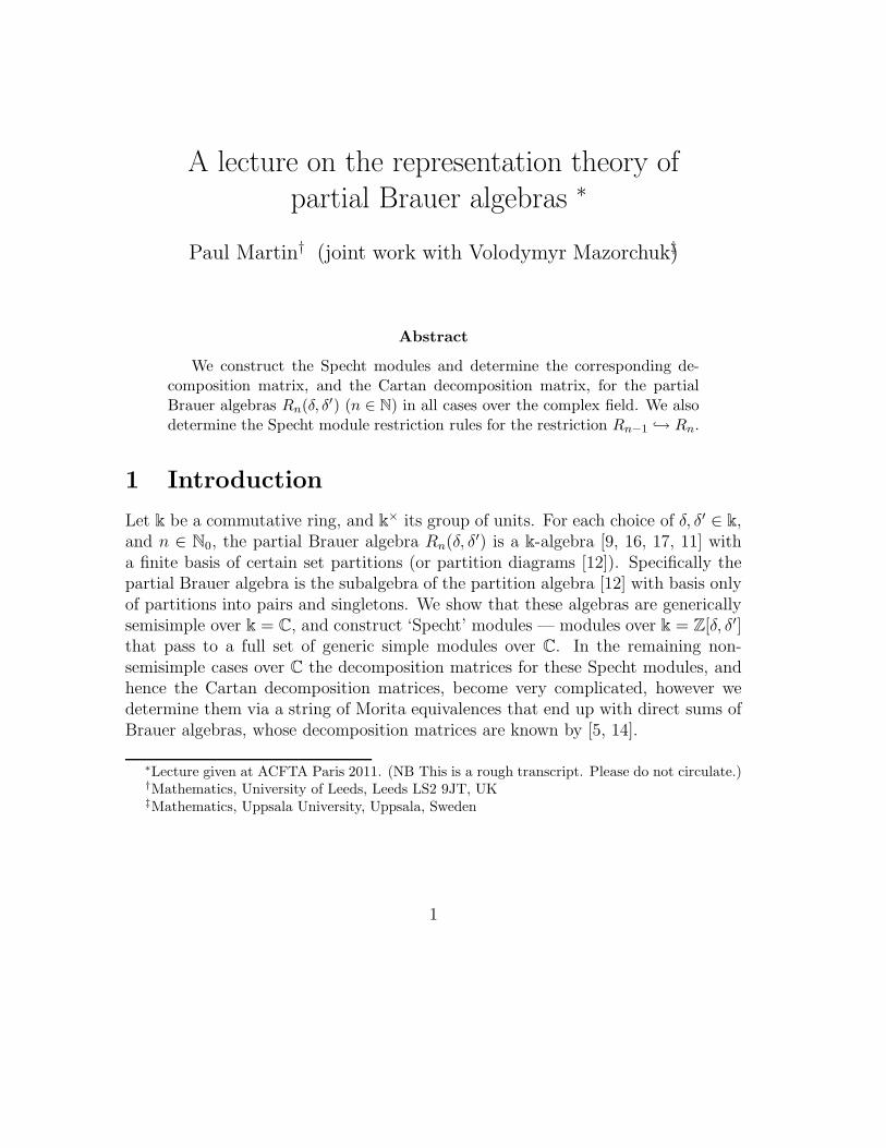
Figure 1: (a) Brauer diagram; (b) Basic composition of partial Brauer partitions(the straightening factor here is δδ′2).

1.1 Between the Brauer algebra and the partition algebra

The partial Brauer algebra is a unital diagram subalgebra of the partition algebra[12] (i.e. a subalgebra with basis a subset of partition diagrams); itself containingthe Brauer algebra [3] as a unital diagram subalgebra. It is convenient to define thepartial Brauer algebra in terms of these classical objects. A Brauer diagram depictstwo rows of n vertices, connected in pairs, as in Figure 1(a). The Brauer algebraBn over k is a k-algebra with a basis of Brauer diagrams. The composition is byfirst juxtaposing diagrams and then applying a straightening rule, i.e. a δ-dependentrule for writing any juxtaposition as an element of the k-span of basis diagrams (see[3]). The Brauer algebra is a subalgebra of the partition algebra Pn, which has abasis consisting of all partitions of the same vertex set (see [12]). There is a largersubalgebra of Pn with basis the set of partitions into pairs and singletons. This hasa 2-parameter version Rn(δ, δ′), with a two-parameter straightening rule: a factor δfor each loop and a factor δ′ for each open string removed. The rule is well illustratedby Figure 1(b), which shows an example from the corresponding diagram category(see also Mazorchuk [16]). This Rn(δ, δ′) is the partial Brauer algebra. We call thediagrams in the corresponding diagram basis partial Brauer diagrams.

1.2 The result

We will use ≡ to denote Morita equivalence. Our key theorem is the following.

2

(1.1) Theorem. For δ′, δ − 1 ∈ k× we have

Rn(δ, δ′) ≡ Bn(δ − 1) ⊕Bn−1(δ − 1)

In §2 we prove this theorem (using a direct analogue of the method used for the par-tition algebra variation treated in [13]). In §3 we combine the theorem with resultson the representation theory of Bn from [14] to describe the complex representationtheory of Rn(δ, δ′). In particular we give an explicit construction for a complete setof Specht modules for Rn(δ, δ′), and show that these are images under the Moritaequivalence of corresponding Brauer Specht modules (or ∆-modules). This means inparticular that we can use the Brauer ∆-decompositon matrices from [14]. Providedthat δ′ is a unit then it can be ‘scaled out’ of representation theoretic calculations,as the theorem suggests. However we also deal with the non-unit cases excepted inthe theorem (see §§4, 5.1).

Acknowledgement. Thanks are due to the Faculty of Natural Sciences of UppsalaUniversity for supporting Paul’s visit to Walter at Uppsala in November 2010 (duringwhich visit this work was mainly done).

2 Constructing the Morita equivalences

In order to construct the Morita equivalences in Theorem 1.1 we will introduce alittle more notation.

2.1 Partition categories

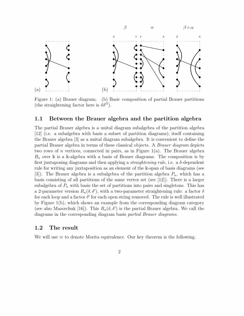
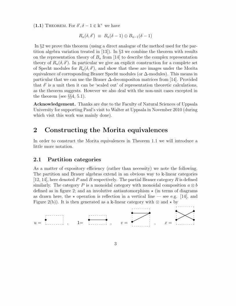
As a matter of expository efficiency (rather than necessity) we note the following.The partition and Brauer algebras extend in an obvious way to k-linear categories[12, 14], here denoted P and B respectively. The partial Brauer category R is definedsimilarly. The category P is a monoidal category with monoidal composition a⊗ bdefined as in figure 2; and an involutive antiautomorphism ⋆ (in terms of diagramsas drawn here, the ⋆ operation is reflection in a vertical line — see e.g. [14], andFigure 2(b)). It is then generated as a k-linear category with ⊗ and ⋆ by

u =•

, 11=• •

, v = •

• •

, x =•

•

•

•

3

(a)

⊗ =

•

•

••••

•••

•

•

•

•

•

••••

•••

•

•

•

(b)

• ⋆7→ •

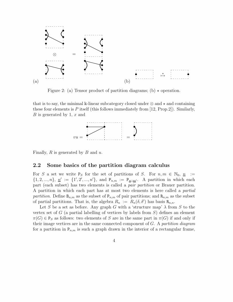
Figure 2: (a) Tensor product of partition diagrams; (b) ⋆ operation.

that is to say, the minimal k-linear subcategory closed under ⊗ and ⋆ and containingthese four elements is P itself (this follows immediately from [12, Prop.2]). Similarly,B is generated by 1, x and

vu = •

• •

= •

•

Finally, R is generated by B and u.

2.2 Some basics of the partition diagram calculus

For S a set we write PS for the set of partitions of S. For n,m ∈ N0, n :={1, 2, ..., n}, n′ := {1′, 2′, ..., n′}, and Pn,m := Pn∪m′ . A partition in which eachpart (each subset) has two elements is called a pair partition or Brauer partition.A partition in which each part has at most two elements is here called a partialpartition. Define Bn,m as the subset of Pn,m of pair partitions; and Rn,m as the subsetof partial partitions. That is, the algebra Rn := Rn(δ, δ′) has basis Rn,n.

Let S be a set as before. Any graph G with a ‘structure map’ λ from S to thevertex set of G (a partial labelling of vertices by labels from S) defines an elementπ(G) ∈ PS as follows: two elements of S are in the same part in π(G) if and only iftheir image vertices are in the same connected component of G. A partition diagramfor a partition in Pn,m is such a graph drawn in the interior of a rectangular frame,

4

in which the vertices are arranged on two opposite edges of the frame, and λ is abijection.

In a partition diagram or Brauer diagram d, say, a part with vertices in both edgesis called a propagating part or a propagating line. The number #p(d) of propagatinglines is called the propagating number (in the literature this is sometimes also knownas rank).

When two diagrams d, d′ are concatenated in composition, we call the ‘middle’layer formed (before straightening) the equator. We write d|d′ for the concatenatedunstraightened ‘diagram’.

The following elementary exercise will illustrate the diagram calculus machinery,and also be useful later on. Define R

+(l)n,n as the subset of partial partitions with l

singletons. For d ∈ R+(l)n,n and d′ ∈ R

+(l′)n,n then the singletons from d and d′ appear in

d|d′ in three possible ways: (i) in the exterior (becoming singletons of dd′); (ii) asendpoints of open strings in the equator, i.e. in pairs connected by a (possibly zerolength) chain of pair parts; (iii) as endpoints of chains terminating in the exterior.

Let 2m be the number of singletons in d|d′ of type-(ii). Then

dd′ ∈ kδ′mR

+(l+l′−2m)n,n (1)

One should keep in mind that every partial Brauer diagram d encodes a partition.Thus the assertion {i, j} ∈ d means that there is a line between vertices i and j ind. If {i, j} ∈ d then one can decompose partition d as

d = {{i, j}} ∪ d′ where d′ = d− {i, j} (2)

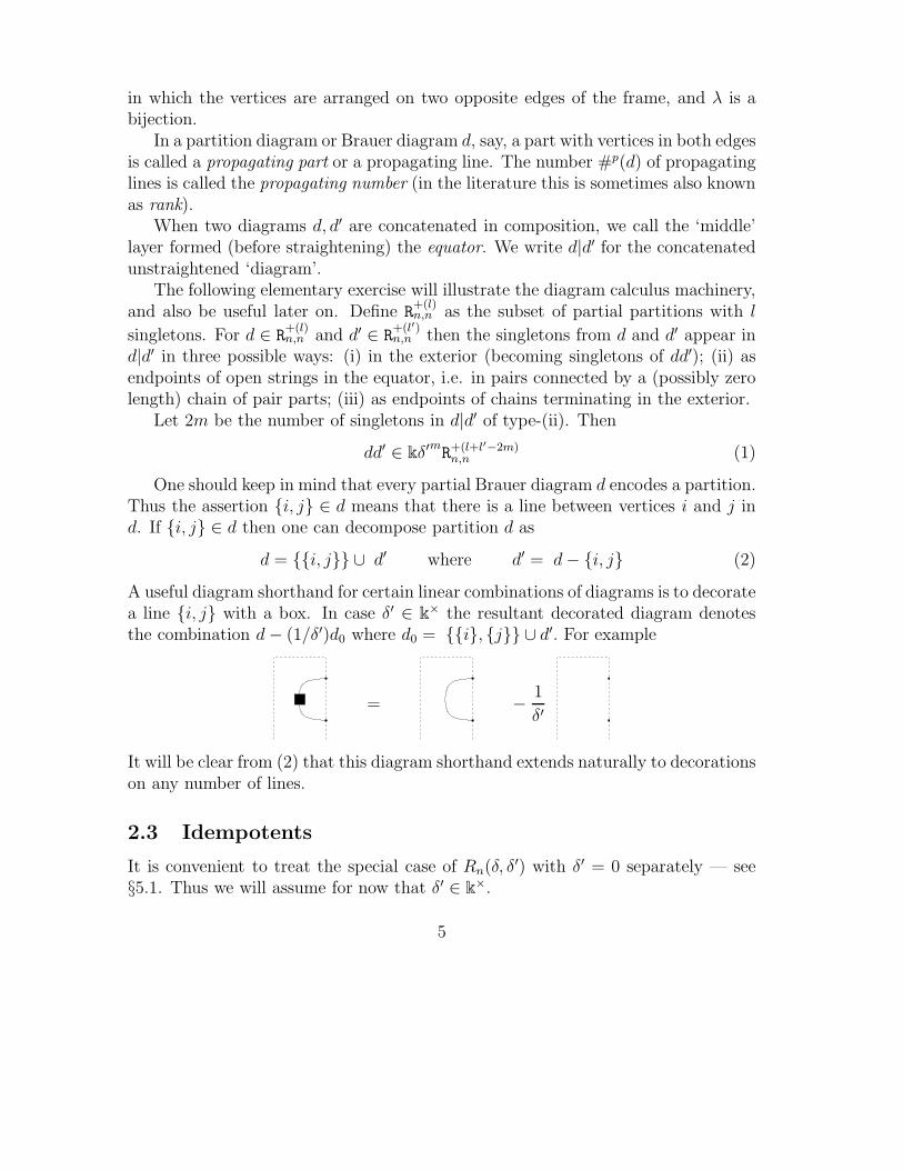
A useful diagram shorthand for certain linear combinations of diagrams is to decoratea line {i, j} with a box. In case δ′ ∈ k× the resultant decorated diagram denotesthe combination d− (1/δ′)d0 where d0 = {{i}, {j}} ∪ d′. For example

= −1

δ′

It will be clear from (2) that this diagram shorthand extends naturally to decorationson any number of lines.

2.3 Idempotents

It is convenient to treat the special case of Rn(δ, δ′) with δ′ = 0 separately — see§5.1. Thus we will assume for now that δ′ ∈ k×.

5

(2.1) For δ′ ∈ k×, define a map 〈〉 : Rn,n → Rn that takes diagram d to the linearcombination 〈d〉 obtained by decorating every line with a box.

For example, with U := uu⋆ ∈ R1,1 we have:

〈11 ⊗ 11〉 = (11 −1

δ′U) ⊗ (11 −

1

δ′U) = 11 ⊗ 11 −

1

δ′(11 ⊗ U + U ⊗ 11) +

1

δ′2U ⊗ U

We can alternatively represent 〈d〉 simply using the diagram for d itself, with theboxes implicit. We call this the ‘ψ-realisation’. Of course in this case diagrams willhave a different composition rule — in this role, we call them ψ-diagrams.

(2.2) Lemma. For δ′ ∈ k×, another basis for Rn(δ, δ′) is 〈Rn,n〉.

Proof. The coefficient matrix for 〈Rn,n〉 in the Rn,n basis is upper-unitriangular inany order refining the partial order by number of pair parts of d. 2

(2.3) Lemma. For d, d′ ∈ Rn,n, the product 〈d〉〈d′〉 in Rn(δ, δ′) is given by:

〈d〉〈d′〉 =

0 if, when the (decorated) diagrams 〈d〉, 〈d′〉 areconcatenated, a singleton part meets a pair part,

〈dd′〉|δ;δ−1 otherwise

Here δ ; δ − 1 means that the factor associated to a closed loop is δ − 1 not δ.

Proof. Let d, d ∈ Rn,n. Recall that if a line from d meets a line from d′ in concate-nation then the composite is a line in the product dd′ (as per Figure 1). Passingto 〈d〉, 〈d′〉 these two lines are replaced by decorated lines. But by the idempotentproperty

(11 −1

δ′U)(11 −

1

δ′U) = (11 −

1

δ′U)

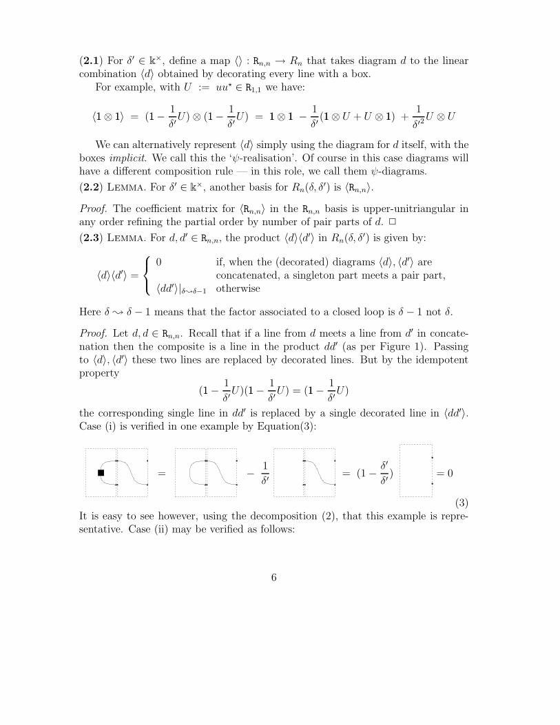
the corresponding single line in dd′ is replaced by a single decorated line in 〈dd′〉.Case (i) is verified in one example by Equation(3):

= −1

δ′= (1 −

δ′

δ′) = 0

(3)It is easy to see however, using the decomposition (2), that this example is repre-sentative. Case (ii) may be verified as follows:

6

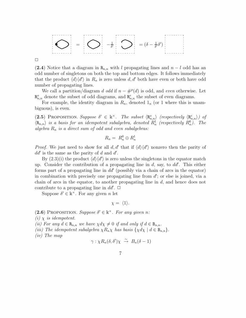
= − 1δ′

= (δ − 1δ′δ′)

2

(2.4) Notice that a diagram in Rn,n with l propagating lines and n − l odd has anodd number of singletons on both the top and bottom edges. It follows immediatelythat the product 〈d〉〈d′〉 in Rn is zero unless d, d′ both have even or both have oddnumber of propagating lines.

We call a partition/diagram d odd if n− #p(d) is odd, and even otherwise. LetR

on,n denote the subset of odd diagrams, and R

en,n the subset of even diagrams.

For example, the identity diagram in Rn, denoted 1n (or 1 where this is unam-biguous), is even.

(2.5) Proposition. Suppose δ′ ∈ k×. The subset 〈Ron,n〉 (respectively 〈Re

n,n〉) of〈Rn,n〉 is a basis for an idempotent subalgebra, denoted R1

n (respectively R0n). The

algebra Rn is a direct sum of odd and even subalgebras:

Rn = R0n ⊕ R1

n

Proof. We just need to show for all d, d′ that if 〈d〉〈d′〉 nonzero then the parity ofdd′ is the same as the parity of d and d′.

By (2.3)(i) the product 〈d〉〈d′〉 is zero unless the singletons in the equator matchup. Consider the contribution of a propagating line in d, say, to dd′. This eitherforms part of a propagating line in dd′ (possibly via a chain of arcs in the equator)in combination with precisely one propagating line from d′; or else is joined, via achain of arcs in the equator, to another propagating line in d, and hence does notcontribute to a propagating line in dd′. 2

Suppose δ′ ∈ k×. For any given n let

χ = 〈1〉.

(2.6) Proposition. Suppose δ′ ∈ k×. For any given n:(i) χ is idempotent.(ii) For any d ∈ Rn,n we have χdχ 6= 0 if and only if d ∈ Bn,n.(iii) The idempotent subalgebra χRnχ has basis {χdχ | d ∈ Bn,n}.(iv) The map

γ : χRn(δ, δ′)χ∼→ Bn(δ − 1)

7

given on the basis by χdχ 7→ d is a k-algebra isomorphism.

Proof. (i) follows from the definition. (ii) follows from Lemma 2.3. (iii) follows from(ii); and (iv) from (iii) and Lemma 2.3. 2

2.4 Idempotent induction functors

(2.7) Consider the usual idempotent induction functor construction (see e.g. [8])

χRnχ−modGχ

--

Rn − modFχ

nn

Gχ : M 7→ Rnχ⊗χRnχ M Fχ : N 7→ χRn ⊗RnN ∼= χN

By (2.6), this construction relates Bn(δ − 1) and Rn(δ). This is directly analogousto the partition algebra case [13]. However a significant difference with the partitionalgebra case is that Rnχ ⊗ χRn 6∼= Rn, so Bn-mod fully embeds in but is notMorita equivalent to Rn-mod. Our main task in determining the structure of Rn isto deal with this difference. In fact, by the construction of R1

n,

χR1n = R1

nχ = 0

and we have

(2.8) Proposition. Let µ : R0nχ ⊗χRχ χR

0n → R0

nχR0n be the multiplication map.

For δ′, δ − 1 ∈ k×

Rnχ⊗χRχ χRn = R0nχ⊗χRχ χR

0n

µ∼= R0

nχR0n = R0

n

is an isomorphism of R0n-bimodules. That is, the functors Fχ and Gχ induce a

Morita equivalence between R0n(δ) and Bn(δ − 1).

For δ = 1 the failure of isomorphism is a degeneration (in the sense of §4); andthe Morita equivalence is replaced by a saturated full embedding.1

Proof. By a general argument (see e.g. [1, §21 Ex.6] or [6]) it is enough to prove thelast identity. We do this by way of the following Lemma. 2

We write sn for the all-singletons diagram sn = U⊗n in Rn.

1That is, Specht modules are taken to Specht modules (or at least ‘combinatorial Specht mod-ules’ — modules with the same composition factors as Specht modules), with no gaps; but a simplemodule is killed by Fχ. See §4.

8

(2.9) Lemma. For any 〈d〉 in 〈Ren,n〉 there exist x, y ∈ 〈Re

n,n〉 such that

〈d〉 =

{xχy d 6= sn

1δ−1

xχy d = sn

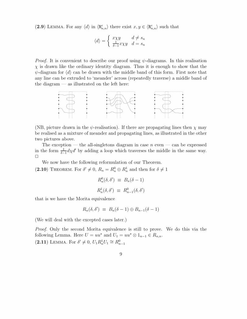
Proof. It is convenient to describe our proof using ψ-diagrams. In this realisationχ is drawn like the ordinary identity diagram. Thus it is enough to show that theψ-diagram for 〈d〉 can be drawn with the middle band of this form. First note thatany line can be extruded to ‘meander’ across (repeatedly traverse) a middle band ofthe diagram — as illustrated on the left here:

(NB, picture drawn in the ψ-realisation). If there are propagating lines then χ maybe realised as a mixture of meander and propagating lines, as illustrated in the othertwo pictures above.

The exception — the all-singletons diagram in case n even — can be expressedin the form 1

δ−1dχd′ by adding a loop which traverses the middle in the same way.

2

We now have the following reformulation of our Theorem.

(2.10) Theorem. For δ′ 6= 0, Rn = R0n ⊕ R1

n and then for δ 6= 1

R0n(δ, δ′) ≡ Bn(δ − 1)

R1n(δ, δ′) ≡ R0

n−1(δ, δ′)

that is we have the Morita equivalence

Rn(δ, δ′) ≡ Bn(δ − 1) ⊕Bn−1(δ − 1)

(We will deal with the excepted cases later.)

Proof. Only the second Morita equivalence is still to prove. We do this via thefollowing Lemma. Here U = uu⋆ and U1 = uu⋆ ⊗ 1n−1 ∈ Rn,n.

(2.11) Lemma. For δ′ 6= 0, U1R1nU1

∼= R0n−1

9

Proof. Consider the augmented basis 〈Ron,n〉 of R1

n. Since this is the odd part, eachdiagram d has an odd number of singleton vertices top and bottom (left and rightas we are drawing it). But in each case one of these vertices must match up withthe singleton in U1, else U1dU1 = 0. The map is to ignore these vertices, so that weend up with a diagram in Rn−1, which then has an even number of singletons, andhence is an even diagram. It is clear that all even (n−1)-diagrams arise in this way.2

(2.12) Lemma. For δ′ 6= 0, the multiplication map µ : R1nU1 ⊗UR1

nU U1R1n

∼→ R1

n isa R1

n-bimodule isomorphism.

Proof. Since R1n is spanned by diagrams with at least one singleton, and hence with

no more than n−1 propagating lines, we can always express them in the form aU1b,that is, R1

nU1R1n = R1

n. Now use the same argument as for Proposition 2.8. 2

It follows from (2.11) that R1nU1 is a left-R1

n right-R0n−1-module; and from (2.12)

that GU = (R1nU1 ⊗R0

n−1−) is a Morita equivalence functor. This concludes the

proof of the Theorem. 2

In short this, together with the construction of Rn-Specht modules which wegive in §3.4, reduces the representation theory of Rn to a problem whose solution isknown. The remainder of the paper is concerned with extracting this representationtheory in practice. (And dealing with the couple of special cases excluded above.)

2.5 Applying the Morita equivalence

(2.13) Recall that if A,B are Morita equivalent finite dimensional algebras overa field then there is a bijection between the sets of equivalence classes of simplemodules; and this induces an identification of Cartan decomposition matrices [2].

(2.14) For each Brauer algebra over C the Cartan decomposition matrix C is de-termined in [14] (using heavy machinery such as [5, ?, ?]). Thus theorem 2.10 andtheorem 2.13 determine the Cartan decomposition matrix CR for Rn over C forδ′, δ − 1 ∈ k×.

However, knowledge of CR does not lead directly to constructions for simpleor indecomposable projective modules, or simple characters. To facilitate this forRn it is convenient to introduce an intermediate class of modules with a concreteconstruction, and to tie these also to the Brauer algebra case. In [14] the Cartan de-composition matrix is determined in the framework of a splitting π-modular system(in the sense of Brauer’s modular representation theory, although the prime π here

10

is a linear monic not a prime number). That is, the Brauer–Specht module decom-position matrix D, which gives the simple content of ‘modular’ reductions of the liftsof generic (i.e. in this case δ-indeterminate) simple modules, is determined. TheMorita equivalence gives a correspondence between Brauer–Specht modules ∆B

n (λ)of Bn and corresponding modules for Rn, thus it only remains to cast the partialBrauer algebras in the same framework and construct their Brauer–Specht modules∆R

n (λ); and show that each Gχ.∆Bn (λ) = ∆R

n (λ).

3 Specht modules for Rn

We call the case of Rn over Z[δ, δ′] the integral case. We want to construct a set ofmodules in the integral case that pass, on extending to a suitable field, to a completeset of simple modules. Our construction for these partial Brauer Specht modules(or ∆-modules) is closely analogous to the construction for the partition and Braueralgebras.

(3.1) It is convenient to write ◦ for the bare composition of diagrams (i.e. ignoringfactors of δ). Define

Rln,m := Rn,l ◦ Rl,m ⊂ Rn,m

Note that this is the subset of partial partitions with at most l propagating lines.Define

R=ln,m = R

ln,m \ Rl−1

n,m

(3.2) Examples: R=11,1 = {11}; while R

=22,2 = {12, x} (with 12 := 11 ⊗ 11). Note that

(R=nn,n, ◦) gives a copy of the symmetric group Sn.

(3.3) Proposition. For any δ, δ′ ∈ k we have that

kRn,n ⊃ kRn−1n,n ⊃ kRn−2

n,n ⊃ ... ⊃ kR0n,n (4)

is a chain of two-sided ideals in Rn. The l-th ideal is generated by U l = U⊗l. Thatis

kRn−ln,n = RnU

lRn

The section kRln,n/kR

l−1n,n in (4) has basis R

=ln,n. Let us write R

l/n,n for this section

of the regular bimodule. 2

(3.4) Note that a bimodule Rl/n,m may be defined similarly starting from Rn,m. In

particular Rl/n,l has the nice property that its basis consists of all diagrams in R

ln,l

such that each vertex on the bottom edge is in a distinct propagating part.

11

(3.5) We may consider the parts of p ∈ Pn,m that meet the top set of vertices tobe totally ordered by the natural order of their lowest numbered elements (from thetop set). We may define a corresponding order for parts that meet the bottom setof vertices. We say that p is non-permuting if the subset of propagating parts hasthe same order from the top and from the bottom.

For a partition in Rn,m, the property of being non-permuting is the same ashaving a diagram with no crossing propagating lines.

(3.6) Let R||l,n denote the subset of R=l

l,n of non-permuting partitions.

(3.7) Lemma. As a left-module

Rl/n,n

∼=⊕

w∈R||l,n

Rl/n,lw

Every summand is isomorphic to Rl/n,l. We have that R=l

n,l is a basis for Rl/n,l, and

R=ln,l = R

||n,l ◦ R

=ll,l (5)

where R=ll,l = Sl. 2

(3.8) Note that Rl/n,l is also a free right kSl-module in a natural way. For each λ ⊢ l

let us choose an element fλ ∈ kSl such that

Sλ = kSlfλ (6)

is the corresponding Specht module [10]. Then define ‘inflation’

∆n(λ) := Rl/n,lfλ

Including fλ ∈ kSl in Rl in the obvious way allows us to draw a picture for this —see for example Fig.3.

(3.9) Proposition. For each basis b(λ) of Sλ there is a basis

bR(λ) = {rb | (r, b) ∈ R||n,l × b(λ)}

of ∆n(λ).

Proof. Note that the module is spanned by elements of form abfλ where a ∈ R||n,l

and b ∈ Sl (consider (5)). 2

12

(3.10) Note that the regular module has a filtration by ∆-modules (cf. [14, Prop.3.4]— a sufficient condition for well-defined filtration multiplicities is char.k = p > 3).Indeed the regular module has a filtration in which all the modules labelled withpartitions of a given degree l (say) are consecutive. Indeed, if k = C (or at leastcontains Q so that kSl is semisimple) the modules {∆n(λ) | λ ⊢ l} do not extendeach other (so can be arranged, among themselves, in any order in the filtration).

(3.11) Define quotient algebra

Rln = Rn/RnU

l+1Rn

(3.12) Note that if δ′ 6= 0 and fλ idempotent (as can always be chosen over C) then

RnUn−|λ|fλ is a projective Rn-module; and R

n−|λ|n Un−|λ|fλ is an indecomposable

projective Rn−|λ|n -module.

(3.13) Proposition. For δ′ ∈ k×, Rn(δ, δ′) is quasihereditary over C.

Proof. In case δ′ = 1 one readily checks that Un, Un−1, ..., U0 (as in Prop.3.3) are aset of heredity idempotents [6]. Other cases are similar. 2

3.1 Images of ∆-modules under the Morita equivalence

We have given a simple concrete construction for the ∆-modules of Rn(δ, δ′). LetΛl denote the set of integer partitions of l; Λ the set of all integer partitions; andΛn = ∪l∈{n,n−2,...}Λl. We will see that over C the modules {∆n(λ) : λ ∈ Λn ∪Λn−1}are, for generic δ, δ′ ∈ C, a complete set of simple modules for Rn. Thus if DR

is the decomposition matrix for these modules for some k and δ, δ′ ∈ k then C =DR(DR)T is the Cartan decomposition matrix (see e.g. [2]). Next we show thatthese modules are the images of the ∆-modules of the appropriate Brauer algebra(generally denoted ∆B

n (λ) here) under the Morita equivalence, and hence determineDR for k = C.

Note that the modules Rl/n,l and so on have direct correspondents in the Brauer

algebra case, so long as n − l is even. Accordingly we use the notation Bl/n,l and so

on there. Thus (see e.g. [5]) for each l ∈ {n, n− 2, ...}, for each λ ⊢ l:

∆Bn (λ) = B

l/n,lfλ

with basisbB(λ) = {db | d ∈ B

||n,l, b ∈ b(λ)}. (7)

13

Applying the (exact) ME functors we get the following. Firstly

χRn ⊗Rn∆n(λ) = χ⊗Rn

χ∆n(λ) = χ⊗Rnχ∆B

n (λ) ∼= ∆Bn (λ) (8)

where we note that χ kills all the diagrams with singletons in the basis bR(λ) for∆n(λ); and in effect simply decorates all the lines on other diagrams. The lastisomorphism then follows on comparing bases, noting that Bn is to be considered inits χRnχ realisation (in which χ acts like 1).

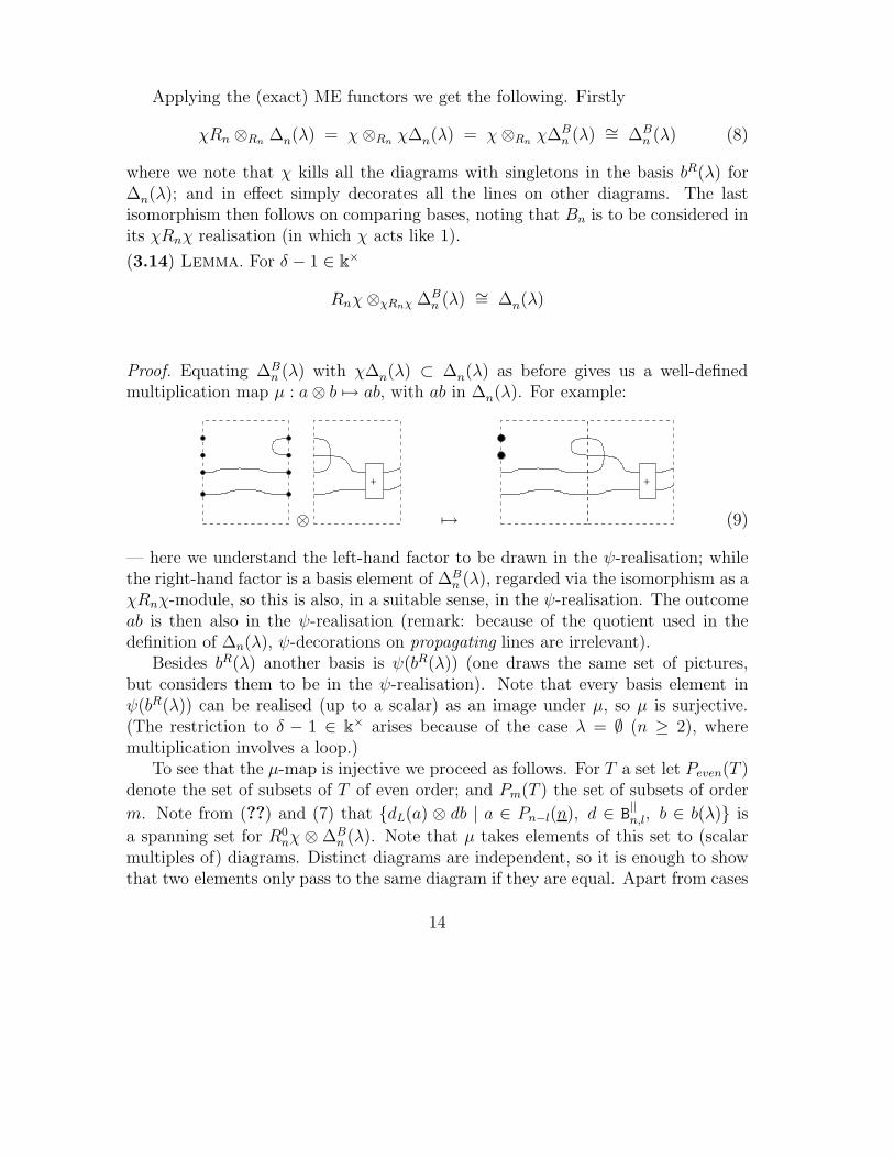
(3.14) Lemma. For δ − 1 ∈ k×

Rnχ⊗χRnχ ∆Bn (λ) ∼= ∆n(λ)

Proof. Equating ∆Bn (λ) with χ∆n(λ) ⊂ ∆n(λ) as before gives us a well-defined

multiplication map µ : a⊗ b 7→ ab, with ab in ∆n(λ). For example:

⊗

+

7→

+

(9)

— here we understand the left-hand factor to be drawn in the ψ-realisation; whilethe right-hand factor is a basis element of ∆B

n (λ), regarded via the isomorphism as aχRnχ-module, so this is also, in a suitable sense, in the ψ-realisation. The outcomeab is then also in the ψ-realisation (remark: because of the quotient used in thedefinition of ∆n(λ), ψ-decorations on propagating lines are irrelevant).

Besides bR(λ) another basis is ψ(bR(λ)) (one draws the same set of pictures,but considers them to be in the ψ-realisation). Note that every basis element inψ(bR(λ)) can be realised (up to a scalar) as an image under µ, so µ is surjective.(The restriction to δ − 1 ∈ k× arises because of the case λ = ∅ (n ≥ 2), wheremultiplication involves a loop.)

To see that the µ-map is injective we proceed as follows. For T a set let Peven(T )denote the set of subsets of T of even order; and Pm(T ) the set of subsets of order

m. Note from (??) and (7) that {dL(a) ⊗ db | a ∈ Pn−l(n), d ∈ B||n,l, b ∈ b(λ)} is

a spanning set for R0nχ ⊗ ∆B

n (λ). Note that µ takes elements of this set to (scalarmultiples of) diagrams. Distinct diagrams are independent, so it is enough to showthat two elements only pass to the same diagram if they are equal. Apart from cases

14

where dL(a) ⊗ db = 0 (due to too few propagating lines), no two diagrams dL(a)give rise to the same image since they have singletons in different positions. On theother hand, if two elements have the same dL(a) factor then they are the same onlyif their ‘Brauer diagram part’ (the lines from dL(a) and the factor db) is the same.But this part passes through the tensor product so they are then (possibly up to ascalar) the same element. 2

3.2 Representation theory examples

We conclude with a few examples illustrating how to import results from Bn(γ)representation theory in practice. (We use γ rather than the usual δ as the parameterhere to avoid confusion with our δ.)

A convenient way to summarize the complex representation theory of Bn(γ) (γ ∈C) is for each integer partition λ to describe the nonzero entries in the correspondingrow of the ∆B-decomposition matrix D. That is,

Dλ,µ = [∆B(µ) : LB(λ)]γ

gives the multiplicity of simple Bn(γ)-module LB(λ) (the simple head of ∆B(λ)) asa composition factor of ∆B(µ). Characterised in this way, we can treat all n at once.We restrict attention to γ ∈ Z since all other cases are semisimple. For such a γ,matrix D may then be given as follows [15].

First we define the map e : R × Λ → RN by

e(γ, λ) = λ− (0, 1, 2, ...) −γ

2(1, 1, 1, ...)

The image e(R,Λ) is a set of strongly decreasing sequences, such as

e(2, (4, 1)) = (3,−1,−3,−4, ...),

but it includes sequences with pairs of terms of equal magnitude (as in the example).Those sequences without any such pairs are said to be regular. For v a sequencein e(R,Λ) we define Reg(v) as the (regular) sequence obtained by deleting all suchpairs. For v regular we define o(v) as the list of ‘signed’ positions in the magnitudeorder of terms in v. The sign of o(v)i is the sign of vi unless vi = 0 in which case itis chosen so that there are an even number of positives. Note in any case that o(v)is now a descending signed permutation of (−1,−2,−3, ...). We define a subset ofN from this o(v), denoted o(v)|+, by keeping the positive terms, except toggling thepresence of 1 if necessary to have a set of even order. Using this we define

oγ(λ) = o(Reg(e(γ, λ)))|+.

15

For example, o2((32)) = {1, 2}. Note that oγ(λ) is a (finite) element of the power

set P (N). To any q ∈ P (N) we associate a binary sequence b ∈ {0, 1}N by bi = 1 ifi ∈ q; and bi = 0 otherwise. We hence associate a binary sequence bγ(λ) ∈ {0, 1}N

to oγ(λ) (one may omit the infinite string of 0s on the right).The next step in the determination of the decomposition matrix D for Bn(γ)

is, for each λ, to pair certain terms in the {0, 1}-sequence bγ(λ), as follows. Everyadjacent 01 is paired. Every 0...1 between which are only paired terms is paired;and this step is iterated. If there is a 1...1 between which are only paired terms,where the first 1 is the first unpaired term, then these 1s are paired; and thisstep is iterated (see [14] for examples). Using this construction we may define acertain hypercubical digraph on a subset of P (N), with oγ(λ) at the head. Eachdescending edge corresponds to toggling a pair, either 01 to 10, or 11 to 00. Theresultant collection of elements of P (N) occur at most once each in this construction.Each element is oγ(µ) for some µ ∈ [λ]γ, where [λ]γ is the block of λ (this can becharacterised as the orbit of elements in Λ whose images under e(γ,−) are relatedby a sequence of signed permutations [5]). Indeed fixing a block by a choice of λ wemay define oλ

γ : Peven(N) → Λ to take oγ(µ) to µ [15].Finally let hγ(λ) denote the hypercube regarded as a (partially ordered) set of

these µs. For example, (32) ∈ [∅]2 and o2((32)) = {1, 2}, so the corresponding

hypercube contains only (32) and o∅2(∅) = ∅.For λ, µ ∈ Λ, define (hγ(λ) : µ) as the number of times µ appears in hγ(λ) (i.e.

either 1 or 0). Then

(3.15) Theorem. [15] For given γ,

DλT µT = [∆B(µT ) : LB(λT )]γ = (hγ(λ) : µ)

2

Combining with Theorem 2.10 and the results of Section 3.1 we have

(3.16) Theorem. Fix δ′ ∈ k×. The λT -row of the Rn(δ, δ′) ∆-decomposition matrixDR for δ = γ+1 contains a 1 in the µT -column for each µ ∈ hγ(λ); and zero otherwise.That is

[∆(µT ) : L(λT )]δ = (hδ−1(λ) : µ)

(NB, besides δ = γ + 1, the other difference from Bn(γ) is the range of values ofλ, µ). 2

(3.17) Consider the example o2((32)) again. One readily checks that among λs with

|λ| ≤ 6, hγ((32)) is the only hγ(λ) containing µ = ∅ (besides hγ(∅) itself); and since

16

δ− 1 = γ = 2 here, giving δ = 3 in the Morita equivalent part of Rn(δ, δ′), this tellsus, for example, that

0 → L6((23)) → ∆6(∅) → L6(∅) → 0

is a short exact sequence of R6(3, δ′)-modules; where Ln(λ) is the corresponding

simple head of ∆n(λ). The dimensions of L6((23)) = ∆6((2

3)) and ∆6(∅) are clearfrom our construction, so this determines also the dimension of the other simple.

This concludes the analysis of the main body of complex representation theoryof Rn.

We now turn to the excepted cases. This is not only for completeness. Theyexhibit some very interesting properties, as we shall now start to explain.

4 Representation theory in the case δ = 1, δ′ 6= 0

The Brauer algebra in case γ = 0 is special in that (for n even) there is one fewersimple module than ∆B-modules (noting that simple modules are counted up to iso-morphism, whereas the set of ∆B-modules has a construction formally independentof such checks). Indeed for n = 2, γ = 0, ∆B

2 ((2))∼→ ∆B

2 (∅).On the other hand γ = 0 is also the case δ − 1 = γ = 0 where our Morita

equivalence in Prop.2.8 fails degenerately (in the sense described there: — the claimis that Fχ, Gχ preserve ‘combinatorial’ ∆-modules, but Fχ = χRn ⊗− kills a simplemodule). This is manifested, for example, as follows.

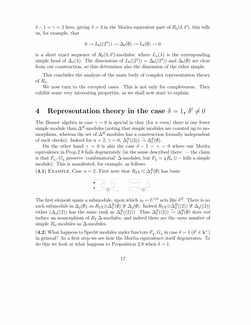
(4.1) Example. Case n = 2. First note that R2χ⊗ ∆B2 (∅) has basis

⊗ , ⊗

The first element spans a submodule, upon which s2 = U⊗2 acts like δ′2. There is nosuch submodule in ∆2(∅), so R2χ⊗∆B

2 (∅) 6∼= ∆2(∅). Indeed R2χ⊗∆B2 ((2)) 6∼= ∆2((2))

either (∆2((2)) has the same rank as ∆B2 ((2))). Thus ∆B

2 ((2))∼→ ∆B

2 (∅) does notinduce an isomorphism of R2 ∆-modules; and indeed there are the same number ofsimple Rn-modules as ∆-modules.

(4.2) What happens to Specht modules under functors Fχ, Gχ in case δ = 1 (δ′ ∈ k×)in general? As a first step we see how the Morita equivalence itself degenerates. Todo this we look at what happens to Proposition 2.8 when δ = 1.

17

Write Reven′

n,n for Revenn,n excluding the all-singletons diagram sn = U⊗n. For δ = 1

we see that kψ(Reven′

n,n ) = RnχRn is a proper ideal in R0n. We have a non-split short

exact sequence of bimodules

0 → RnχRn → R0n → R0

n/RnχRn → 0 (10)

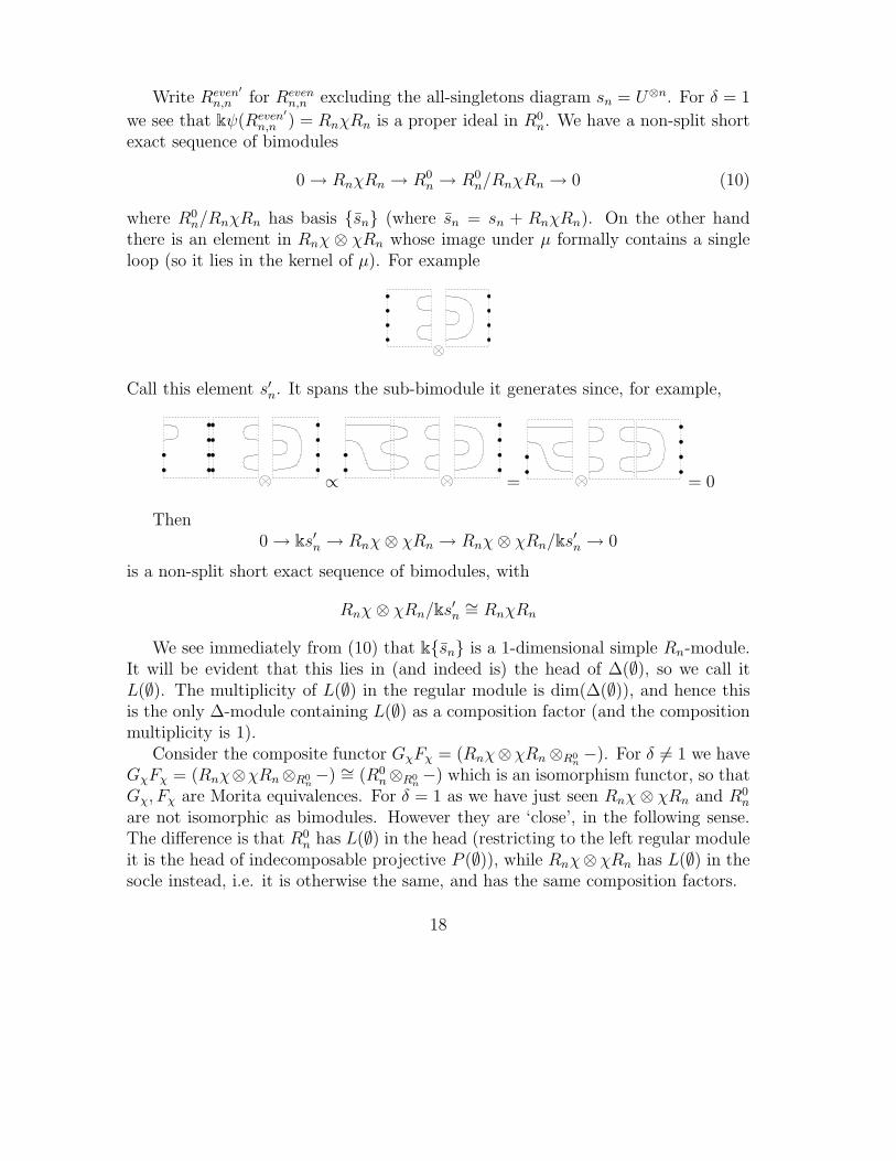
where R0n/RnχRn has basis {s̄n} (where s̄n = sn + RnχRn). On the other hand

there is an element in Rnχ ⊗ χRn whose image under µ formally contains a singleloop (so it lies in the kernel of µ). For example

Call this element s′n. It spans the sub-bimodule it generates since, for example,

∝ = = 0

Then0 → ks′n → Rnχ⊗ χRn → Rnχ⊗ χRn/ks

′n → 0

is a non-split short exact sequence of bimodules, with

Rnχ⊗ χRn/ks′n∼= RnχRn

We see immediately from (10) that k{s̄n} is a 1-dimensional simple Rn-module.It will be evident that this lies in (and indeed is) the head of ∆(∅), so we call itL(∅). The multiplicity of L(∅) in the regular module is dim(∆(∅)), and hence thisis the only ∆-module containing L(∅) as a composition factor (and the compositionmultiplicity is 1).

Consider the composite functor GχFχ = (Rnχ⊗χRn ⊗R0n−). For δ 6= 1 we have

GχFχ = (Rnχ⊗χRn⊗R0n−) ∼= (R0

n⊗R0n−) which is an isomorphism functor, so that

Gχ, Fχ are Morita equivalences. For δ = 1 as we have just seen Rnχ⊗ χRn and R0n

are not isomorphic as bimodules. However they are ‘close’, in the following sense.The difference is that R0

n has L(∅) in the head (restricting to the left regular moduleit is the head of indecomposable projective P (∅)), while Rnχ⊗χRn has L(∅) in thesocle instead, i.e. it is otherwise the same, and has the same composition factors.

18

We have FχL(∅) ∼= χks̄n∼= 0 and, as before, Fχ∆(λ) ∼= ∆B(λ) (any λ).

WHAT’S THIS?:For λ 6= ∅ (and n 6= 2) we have Gχ∆B(λ) ∼= ∆(λ). Finally Gχ∆B(∅) 6∼= ∆(∅),

however Gχ∆B(∅) and ∆(∅) have the same composition factors.Thus (for δ − 1 = γ = 0) the rows of the decomposition matrix not involving ∅

are the same between D and DR (see e.g. [8, §6.6]). The difference is that DR hasa row labelled by ∅. However, as already noted, this row is (1, 0, 0, 0, ...). We havethus shown that for any n

DR = Dformal

(as defined in (4.4)).

4.1 Examples: δ = 1

(4.3) With γ = 0 we get o0(∅) = ∅ and o0((12)) = {1, 2}, so hypercube h0((1

2)) con-tains only (12) and ∅. Formally this implies a ∆B-module homomorphism ∆B

2 ((2)) →∆B

2 (∅), but in case n = 2 both modules are rank-1, and so the implied ∆B-modulehomomorphism is actually an isomorphism, as noted above.

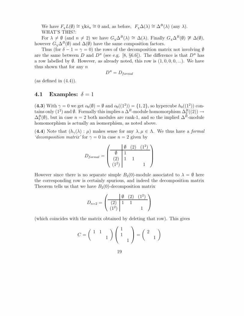
(4.4) Note that (hγ(λ) : µ) makes sense for any λ, µ ∈ Λ. We thus have a formal‘decomposition matrix’ for γ = 0 in case n = 2 given by

Dformal =

∅ (2) (12)∅ 1

(2) 1 1(12) 1

However since there is no separate simple B2(0)-module associated to λ = ∅ herethe corresponding row is certainly spurious, and indeed the decomposition matrixTheorem tells us that we have B2(0)-decomposition matrix

Dn=2 =

∅ (2) (12)(2) 1 1(12) 1

(which coincides with the matrix obtained by deleting that row). This gives

C =

(1 1

1

)

11

1

=

(2

1

)

19

Note that the corresponding λ = ∅ column of Dn=2 is not spurious in this Brauermodular treatment. The module ∆B((2)) is not isomorphic to ∆B(∅) over C[γ] orC(γ) and both are needed as elements of the complete set of simples over C(γ). Theγ = 0 projective P(2), which looks like a self-extension here, lifts to a combination ofnon-isomorphic integral modules. Indeed the primitive idempotent decompositionof 1 in case γ = 0 is 1 = (1 + (12))/2 + (1 − (12))/2, which lifts trivially to C[γ];but the idempotent (1+ (12))/2 does not pass to a primitive idempotent over C(γ),instead passing to a combination of two inequivalent idempotents.

—GO THROUGH BENSON 1.9.6 in THIS CASE!!!—In contrast there is a simple R2(0)-module associated to λ = ∅, and in fact

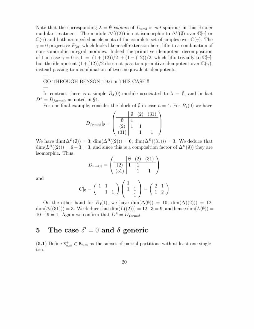
DR = Dformal, as noted in §4.For one final example, consider the block of ∅ in case n = 4. For B4(0) we have

Dformal|∅ =

∅ (2) (31)∅ 1

(2) 1 1(31) 1 1

We have dim(∆B(∅)) = 3; dim(∆B((2))) = 6; dim(∆B((31))) = 3. We deduce thatdim(LB((2))) = 6− 3 = 3, and since this is a composition factor of ∆B(∅)) they areisomorphic. Thus

Dn=4|∅ =

∅ (2) (31)(2) 1 1(31) 1 1

and

C|∅ =

(1 1

1 1

)

11 1

1

=

(2 11 2

)

On the other hand for R4(1), we have dim(∆(∅)) = 10; dim(∆((2))) = 12;dim(∆((31))) = 3. We deduce that dim(L((2))) = 12−3 = 9, and hence dim(L(∅)) =10 − 9 = 1. Again we confirm that DR = Dformal.

5 The case δ′ = 0 and δ generic

(5.1) Define R+n,m ⊂ Rn,m as the subset of partial partitions with at least one single-

ton.

20

(5.2) Lemma. Let k be any commutative ring. Then

RnR+n,nRn = kR+

n,n ∪ δ′Rn

Proof. Any product involving a diagram with a singleton either produces a diagramwith a singleton, or else an open string. This is elementary — see (1). 2

(5.3) In the δ′ = 0 case one sees from (1) that the diagrams with one or moresingleton generate a nilpotent ideal. In determining the simple modules of Rn onecan quotient by this ideal. The quotient can be identified with the Brauer sub-algebra, whose generic representation theory has been studied in [4]; and generalrepresentation theory over C in [5, 14].

(5.4) In §3.4 we give a construction for Specht modules for each partial Braueralgebra. By this we mean modules for the algebra over Z[δ, δ′] that can be madewell-defined over a PID either by fixing δ′ = 1 or by fixing δ to a suitable value; suchthat, over a suitable extension to a field in either case, the set of modules passes to acomplete set of simple modules in a semisimple algebra. This means that we can usethe tools of Brauer’s modular representation theory (here to study non-semisimplespecialisations of the parameters, rather than fields of finite characteristic).

If we consider δ′ = 0 and δ generic, so that the Brauer algebra is semisimple,then we can describe the simple content of Specht modules (and hence the Cartandecomposition matrix). We do this in §??.

5.1 Representation theory in case δ′ = 0

The following proposition on the structure of Specht modules completely determinesthe Cartan decomposition matrix in case δ′ = 0 in all cases in which the Brauersubalgebra is semisimple (e.g. for δ >> n).(Other cases over C are also determined in principle, but one must combine withthe appropriate Brauer algebra representation theory. This is known, but we do notgive an explicit description here.)

(5.5) Recall from (5.3) that the Specht modules of the Brauer algebra are the gener-ically simple modules of Rn(δ, 0). That is to say, they lift to Rn(δ, 0)-modules withthis property.

We assume the reader is familiar with these modules.

21

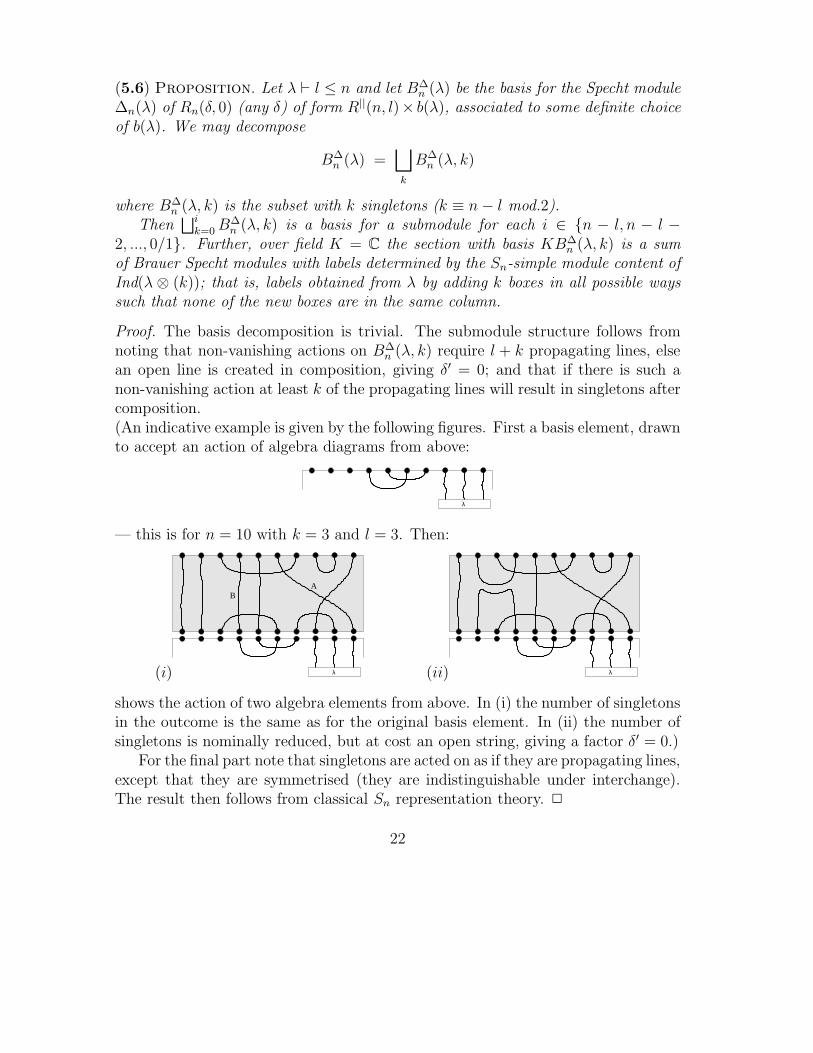
(5.6) Proposition. Let λ ⊢ l ≤ n and let B∆n (λ) be the basis for the Specht module

∆n(λ) of Rn(δ, 0) (any δ) of form R||(n, l)× b(λ), associated to some definite choiceof b(λ). We may decompose

B∆n (λ) =

⊔

k

B∆n (λ, k)

where B∆n (λ, k) is the subset with k singletons (k ≡ n− l mod.2).

Then⊔i

k=0B∆n (λ, k) is a basis for a submodule for each i ∈ {n − l, n − l −

2, ..., 0/1}. Further, over field K = C the section with basis KB∆n (λ, k) is a sum

of Brauer Specht modules with labels determined by the Sn-simple module content ofInd(λ ⊗ (k)); that is, labels obtained from λ by adding k boxes in all possible wayssuch that none of the new boxes are in the same column.

Proof. The basis decomposition is trivial. The submodule structure follows fromnoting that non-vanishing actions on B∆

n (λ, k) require l + k propagating lines, elsean open line is created in composition, giving δ′ = 0; and that if there is such anon-vanishing action at least k of the propagating lines will result in singletons aftercomposition.(An indicative example is given by the following figures. First a basis element, drawnto accept an action of algebra diagrams from above:

λ

— this is for n = 10 with k = 3 and l = 3. Then:

(i) λ

AB

(ii) λ

shows the action of two algebra elements from above. In (i) the number of singletonsin the outcome is the same as for the original basis element. In (ii) the number ofsingletons is nominally reduced, but at cost an open string, giving a factor δ′ = 0.)

For the final part note that singletons are acted on as if they are propagating lines,except that they are symmetrised (they are indistinguishable under interchange).The result then follows from classical Sn representation theory. 2

22

6 Branching rules for Specht modules

Here M+ is the incidence matrix of the directed Young graph (this has vertex setΛ; and edge µ ⊳ λ if the Young diagrams differ by a single box).

(6.1) Theorem. The map from Rn to Rn+1 given by d 7→ d ⊗ 1 is an algebrainjection. The restriction rule for Rn+1 ∆-modules to Rn is given by the short exactsequence

0 → ∆n(λ) ⊕Bλ → resn∆n+1(λ) → Cλ → 0

(here and throughout we take ∆n(µ) = 0 if |µ| > n), where

Bλ = ⊕′µ⊳λ∆n(µ); Cλ = ⊕′

µ⊲λ∆n(µ)

(⊕′ denotes a direct sum if k = C, but a not necessarily direct sum for fields of finitecharacteristic). That is

resn∆n+1(λ) =

∆n(λ)︸ ︷︷ ︸

A

⊕ (⊕′µ⊳λ∆n(µ))

︸ ︷︷ ︸

B

+ (⊕′µ⊲λ∆n(µ))

Proof. We assume familiarity with induction and restriction rules for the symmetricgroup [10]. Consider a basis as in Prop.3.9. Separate the basis into three subsets:(1) elements in which the last vertex is a singleton;(2) elements in which the last vertex starts a propagating line;(3) elements in which the last vertex ends an arc from some other vertex.

Now consider the action of Rn. Clearly (1) is a basis for A. Meanwhile (2) is a

basis for the inflation Rl−1/n,l−1resl−1∆λ, which gives B. Finally, modulo A and B, (3)

is a basis for the inflation Rl+1/n,l+1indl+1∆λ.

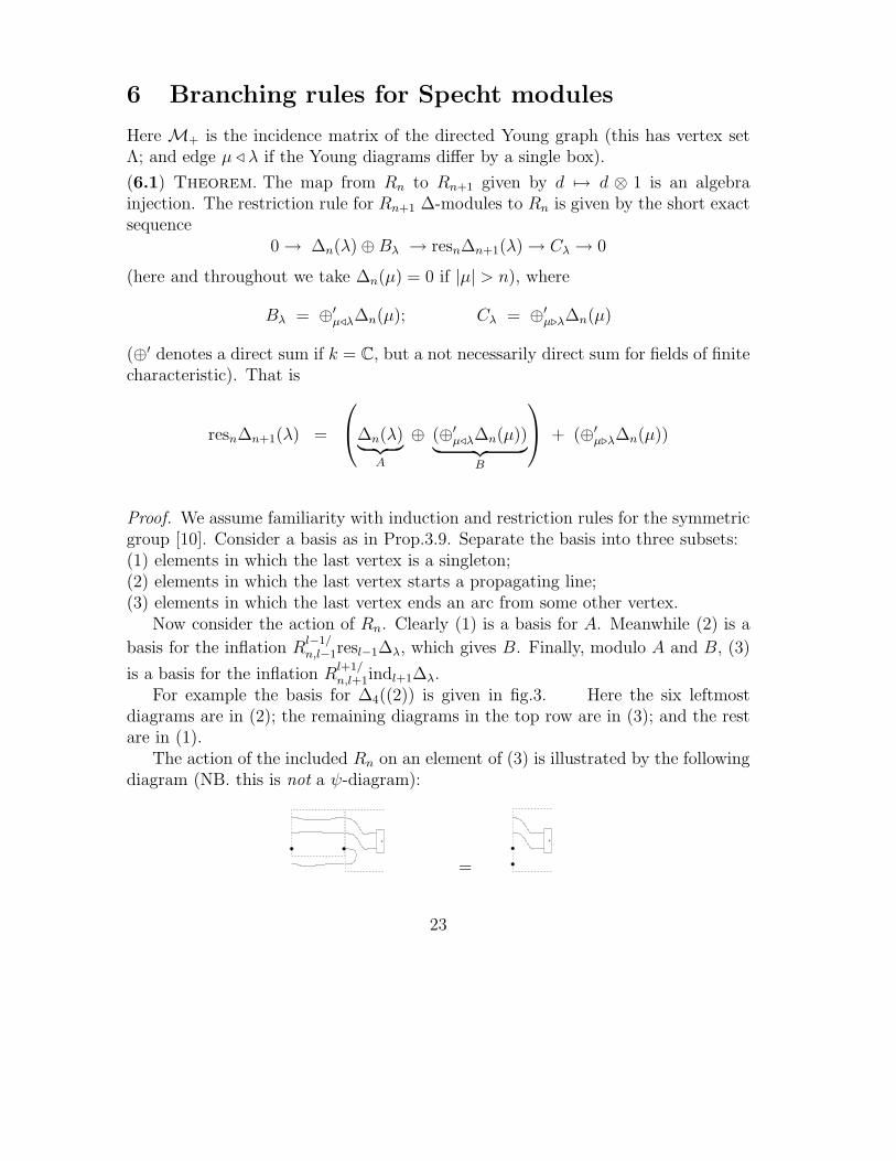
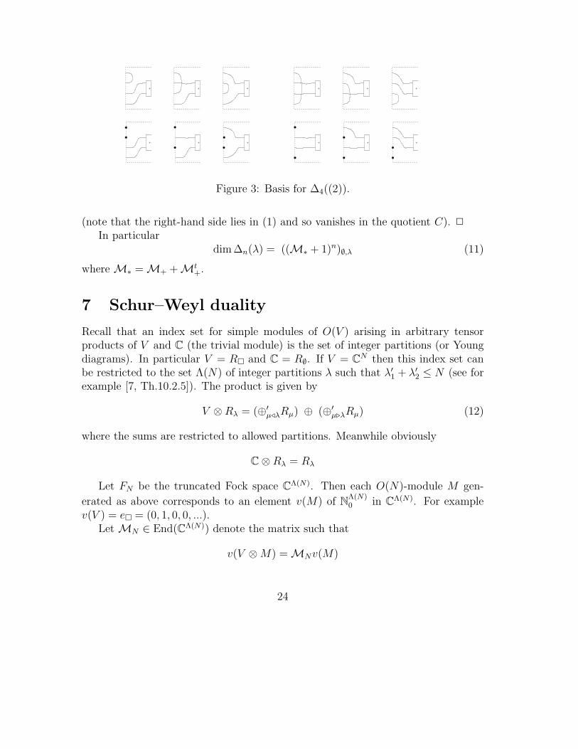
For example the basis for ∆4((2)) is given in fig.3. Here the six leftmostdiagrams are in (2); the remaining diagrams in the top row are in (3); and the restare in (1).

The action of the included Rn on an element of (3) is illustrated by the followingdiagram (NB. this is not a ψ-diagram):

+

=

+

23

+ + + + + +

+ + + + + +

Figure 3: Basis for ∆4((2)).

(note that the right-hand side lies in (1) and so vanishes in the quotient C). 2

In particulardim ∆n(λ) = ((M∗ + 1)n)∅,λ (11)

where M∗ = M+ + Mt+.

7 Schur–Weyl duality

Recall that an index set for simple modules of O(V ) arising in arbitrary tensorproducts of V and C (the trivial module) is the set of integer partitions (or Youngdiagrams). In particular V = R� and C = R∅. If V = CN then this index set canbe restricted to the set Λ(N) of integer partitions λ such that λ′1 + λ′2 ≤ N (see forexample [7, Th.10.2.5]). The product is given by

V ⊗ Rλ = (⊕′µ⊳λRµ) ⊕ (⊕′

µ⊲λRµ) (12)

where the sums are restricted to allowed partitions. Meanwhile obviously

C ⊗ Rλ = Rλ

Let FN be the truncated Fock space CΛ(N). Then each O(N)-module M gen-

erated as above corresponds to an element v(M) of NΛ(N)0 in CΛ(N). For example

v(V ) = e� = (0, 1, 0, 0, ...).Let MN ∈ End(CΛ(N)) denote the matrix such that

v(V ⊗M) = MNv(M)

24

Note that this matrix is well-defined and directly determined by (12). Then of course

v((V ⊕ C) ⊗M) = (MN + 1)v(M)

Also

(7.1) Theorem. The vector (MN + 1)n gives the list of dimensions of simple mod-ules of the commutant EndO(N)((V ⊕ C)n).

(7.2) Theorem. For N >> n we have Rn(N) ∼= EndO(N)((V ⊕ C)n).

Proof. cf. (11), Theorem 7.1. 2

(7.3) The action of Rn on (V ⊕ C)n is.... WHAT?

References

[1] F W Anderson and K R Fuller, Rings and categories of modules, Springer, 1974.

[2] D J Benson, Representations and cohomology I, Cambridge, 1995.

[3] R Brauer, On algebras which are connected with the semi–simple continuousgroups, Annals of Mathematics 38 (1937), 854–872.

[4] W P Brown, An algebra related to the orthogonal group, Michigan Math. J. 3

(1955-56), 1–22.

[5] A G Cox, M De Visscher, and P P Martin, The blocks of the Braueralgebra in characteristic zero, Representation Theory 13 (2009), 272–308,(math.RT/0601387).

[6] V Dlab and C M Ringel, A construction for quasi-hereditary algebras, Compo-sitio Mathematica 70 (1989), 155–175.

[7] R Goodman and N R Wallach, Representations and invariants of the classicalgroups, Cambridge, 1998.

[8] J A Green, Polynomial representations of GLn, Springer-Verlag, Berlin, 1980.

[9] U Grimm and S O Warnaar, Solvable RSOS models based on the dilute BMWalgebra, Nucl Phys B [FS] 435 (1995), 482–504.

[10] G D James and A Kerber, The representation theory of the symmetric group,Addison-Wesley, London, 1981.

25

[11] G Kudryavtseva and V Mazorchuk, On presentations of Brauer-type monoids,Central Europ. J. Math. 4 (2006), no. 3, 413–434.

[12] P P Martin, Temperley–Lieb algebras for non–planar statistical mechanics —the partition algebra construction, Journal of Knot Theory and its Ramifications3 (1994), no. 1, 51–82.

[13] , The partition algebra and the Potts model transfer matrix spectrum inhigh dimensions, J Phys A 32 (2000), 3669–3695.

[14] , The decomposition matrices of the Brauer algebra over the complexfield, preprint (2009), (http://arxiv.org/abs/0908.1500).

[15] , Lecture notes in representation theory, unpublished lecture notes, 2009.

[16] V Mazorchuk, On the structure of Brauer semigroup and its partial analogue,Problems in Algebra 13 (1998), 29–45.

[17] , Endomorphisms of Bn, PBn and Cn, Comm. Algebra 30 (2002), 3489–3513.

26