A. Introduction B. Production of Radionuclides and ...
53
R. Schupfner, Radio analytical Working Methods for Scientists 1 von 53 A. Introduction B. Production of Radionuclides and Radiolabeled Compounds 1. Production in Nuclear Reactors 1.1 Neutron capture reactions (n, γ) 1.2 Nuclear fission (n,f)-reactions 2. Production of Radionuclides applying Particle Accelerators 3. Radionuclide Generators 4. Radiolabeled Compounds 4.1 Labelling Applying Biochemical Methods 4.2 Exchange Reactions 4.3 Specially Aspects of Chemical Behaviour of Radionuclides 4.4 Radionuclides of High specific Activity 4.5 Radiocolloides 4.6 Trace Techniques C. Radioactivity 1. Stability of the Atomic Nucleus 2. Principles of the Radioactive Decay 2.1 Activity versus Time 2.2 Statistics of Radioactive Decay 2.3 Activity and Mass 2.4 Scale Bases of Activity 2.5 Radioactive Decay Chains 3. Modes of Decay and Nuclear Radiation 3.1 α−Radiation 3.2 β− Radiation 3.3 γ− Radiation 3.4 n-Emission 3.5 Summary: Properties of Nuclear Radiation D. Radiation Exposure 1. Harmful Effects of Ionizing Radiation on the Human Body 2. Terms of Dose, Dosimetric Magnitudes, Tissue and Radiation Factors 2.1 Radiation Exposure 2.2 Dose 2.3 Measurements for External Radiation 2.4 Calculation of the Body Dose 2.4.1 Calculation of the organ absorbed dose equivalent H T 2.4.2 Definition of absorbed dose D T,R 2.5 Calculation of the Effective Dose E 2.6 Calculation of Radiation Exposure through Incorporation or Submersion 2.7 Calculation of the External Radiation Exposure of the Unborn Child 2.8 Calculation of the Internal Radiation Exposure of the Unborn Child 2.9 Local Dose H L 2.10 Local Dose Rate Ĥ L 2.11 Calculation of the Organ Committed Dose H T (τ) and the Effective Committed Dose E (τ) 2.11.1 Calculation of the organ committed dose H T (τ) 2.11.2 Calculation of the effective committed dose E(τ) 2.12 Calculation of Doses D E and D T after Incorporation 2.12.1 Dose calculation 2.12.2 Incorporation monitoring 2.12.2.1 Requirement 2.12.2.2 Procedure 2.12.2.3 Example: Standard incorporation monitoring in the case of handling 33 P
Transcript of A. Introduction B. Production of Radionuclides and ...
R. Schupfner, Radio analytical Working Methods for Scientists 1 von 53
A. Introduction B. Production of Radionuclides and Radiolabeled Compounds 1. Production in Nuclear Reactors
1.1 Neutron capture reactions (n, γ) 1.2 Nuclear fission (n,f)-reactions 2. Production of Radionuclides applying Particle Accelerators 3. Radionuclide Generators 4. Radiolabeled Compounds 4.1 Labelling Applying Biochemical Methods 4.2 Exchange Reactions 4.3 Specially Aspects of Chemical Behaviour of Radionuclides 4.4 Radionuclides of High specific Activity 4.5 Radiocolloides 4.6 Trace Techniques
C. Radioactivity
1. Stability of the Atomic Nucleus 2. Principles of the Radioactive Decay 2.1 Activity versus Time 2.2 Statistics of Radioactive Decay 2.3 Activity and Mass 2.4 Scale Bases of Activity 2.5 Radioactive Decay Chains 3. Modes of Decay and Nuclear Radiation
3.1 α−Radiation
3.2 β− Radiation
3.3 γ− Radiation 3.4 n-Emission 3.5 Summary: Properties of Nuclear Radiation
D. Radiation Exposure
1. Harmful Effects of Ionizing Radiation on the Human Body 2. Terms of Dose, Dosimetric Magnitudes, Tissue and Radiation Factors 2.1 Radiation Exposure 2.2 Dose 2.3 Measurements for External Radiation 2.4 Calculation of the Body Dose 2.4.1 Calculation of the organ absorbed dose equivalent HT 2.4.2 Definition of absorbed dose DT,R 2.5 Calculation of the Effective Dose E 2.6 Calculation of Radiation Exposure through Incorporation or Submersion 2.7 Calculation of the External Radiation Exposure of the Unborn Child 2.8 Calculation of the Internal Radiation Exposure of the Unborn Child 2.9 Local Dose HL 2.10 Local Dose Rate ĤL 2.11 Calculation of the Organ Committed Dose HT(τ) and the Effective Committed Dose E (τ) 2.11.1 Calculation of the organ committed dose HT(τ)
2.11.2 Calculation of the effective committed dose E(τ) 2.12 Calculation of Doses DE and DT after Incorporation 2.12.1 Dose calculation 2.12.2 Incorporation monitoring 2.12.2.1 Requirement 2.12.2.2 Procedure 2.12.2.3 Example: Standard incorporation monitoring in the case of handling 33P
R. Schupfner, Radio analytical Working Methods for Scientists 2 von 53
3. Naturally Caused Radiation Exposure of Human E. Legal Foundations of Radiation Protection 1. The double-sided character of radioactivity 2. The Radiation Protection Ordinance (RPO 2.1 Purpose 2.2 Key Aspects
F. Methods of Detection of Nuclear Radiation 1. Single Nuclide Determination 2. Multi Nuclide Determination 3. Determination of Activity 3.1 Basic Radioanalytical Equation
3.2 Counting Efficiency ηPhy
3.3 Calibration Factor κ
3.4 Dead Time tD
3.5 Counting Uncertainty 3.6 Lower Limit of Detection and Detection Limit 4. Methods of Radiation Detection Measurement 4.1 General properties of a radiation detector 4.2 Gas-filled Detectors 4.3 Scintillation Detectors 4.3.1 Fundamentals 4.3.2 Liquid Scintillation Counting (LSC) 4.3.3 Cerenkov-Counting 4.4 Semiconductor Detectors 4.5 Choice of Detectors
5. Spectrometric Methods 5.1 Examples of pulse height spectra 5.2 Full width at half maximum (FWHM) as a measure of energy resolution 6. Neutron Detectors 7. Spatially Resolving Devices 7.1 Photographic Emulsions (Autoradiography) 7.2 Dielectric Trace Detectors 8. Isotopic Dilution Analysis 8.1 Radioactive yield tracer 8.2 Stable Yield Tracers 9. Contamination monitoring (example: CoMo170)
H. Laboratory Course 1. Contamination Monitoring 1.1 Wipe Test and LSC 1.2 Wipe Test and Cerenkcov-counting 1.3 Contamination Monitor 2. Properties of Nuclear Radiation 2.1 Suited Shielding Materials 2.2 Suited Radiation Detection Devices 3. Rules of save handling of unsealed radioactive substances
R. Schupfner, Radio analytical Working Methods for Scientists 3 von 53
App I. Literature [1] H. Lieser, Introduction of Nuclear Chemistry, 2. ed., Verlag Chemie, Weinheim, Deerfield Beach, Florida, Basel, 1980. [2] Kiefer, Koelzer, Radiation Protection, 1988. [3] R. G. Jaeger, Dosimetry and Radiation Protection, Georg Thieme Verlag, Stuttgart, 1959. [4] H. E. Johns, J. R. Cunningham, The Physics of Radiology, Ed. Charles C Thomas, Springfield, Illinois, USA, 3. ed., 1969. [5] Atomic Law (AtG), BGBl. I, Jul,y 15th, 1985. [6] Radiation Protection Ordinance (RPO) Edition 02/12 (bilingual), The German original of this translation was published in Federal Law Gazette, BGBl. I 2001 No.38, its last Amendment 2012, No. 10. [7] G. F. Knoll, Radiation Detection and Measurement, 1987. App II: Declaration The Federal Office for Radiation Protection (Bundesamt für Strahlenschutz - BfS) publishes several laws and regulations on nuclear safety and radiation protection in English. These translations are intended solely as a convenience to the non-German public. Any discrepancies or differences in the translation are not binding and have no legal effect for compliance or enforcement purposes. In case of discrepancies the German official version shall prevail.
R. Schupfner, Radio analytical Working Methods for Scientists 4 von 53
A. Introduction There is a wide range of applications of radionuclides but the effects of ionizing radiation to human tissues can cause severe damage and injuries for example cancer. As a consequence every justified practices including handling of radioactive substances must consider both: the benefit and the risk. The application of radionuclides to life sciences is well established because of high sensitivity and a wide spread possibility of labelling suited compounds. The sensitivity is much higher for radionuclides compared to stable compounds depending on the half life time t1/2 of the radionuclide. The activity A and half life time t1/2 are connected like: A = = λ·N = ·N
N: Number of Nuclei dN: Change of the number of nuclei occurring within the time dt. Table 1 : Detectable amounts of radionuclides of different half life time of an activity of 1 Bq. t1/2 Number of
nuclei N Mol
1 h 5200 8,64·10-21 1 d 125000 2,08·10-19 1 y 4,55·107 7,55·10-17 105 y 4,55·1012 7,55·10-12 109 y 4,55·1016 7,55·10-21 Radionuclides, e.g. 3H, 14C, 32P, 33P, 35S, 45Ca, 125I are applied routinely for labelling chemical compounds in various fields of life sciences. They are named as unsealed radioactive substances according to §3 of the Radiation Protecting Ordinance (RPO). In addition of the application of unsealed radionuclides sealed radionuclides apply the physical properties of ionising radiation. The field of application is manifold, e.g. testing radiators, radiation therapy, disinfection of surgical instruments and food. For these purposes radionuclides are applied as 60Co, 133Ba, 137Cs, 192Ir, 226Ra, 241Am. B. Production of Radionuclides and Radio labelled Compounds Radionuclides can be produced within nuclear reactions. A general equation of nuclear reactions is: A (x, y) B A is the target nucleus x is the projectile y is the particle or photon being emitted B is the produced projectile Dependent on the properties of projectiles and emitted particles one distinguishes the following types of nuclear reactions:
dN dt
ln2 t1/2
R. Schupfner, Radio analytical Working Methods for Scientists 5 von 53
α, 2n α, n
p, 2np, n d, 2n
α, t p, γ
d, nt, n t, p
d, t n, 2n γ, n p,pn
d, p n, γ
t, dt, p
p, α d, αn, d γ, p
n, p d, 2p
n, α
Anzahl der Neutronen N = A-Z
An
za
hl
der
Pro
ton
en
P =
Z
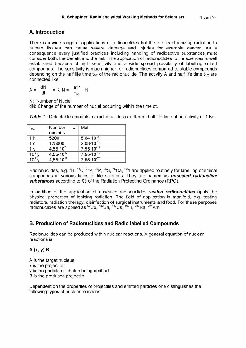
Figure 1: Survey of transitions of radionuclides caused by nuclear reactions. The target nucleus is shaded. To enable such nuclear reactions much energy has to be applied. 1. Production in Nuclear Reactors Radionuclides can be produced within nuclear reactors applying high neutron flux densities of Φ ≈ 1010 to 1016 cm-2·s-1. Radionuclide formation occurs by neutron capture reactions (n, γ) or nuclear fission (n,f). 1.1 Neutron Capture (n, γγγγ) Neutron capture reactions (n, γ) are reactions of type: AZX + n → A+1
ZX* + γ where A: atomic number
Z: nuclear charge number X: target nucleus X*: produced nucleus n: neutron γ: spontaneous emitted gamma-quanta
(n, γ)-reactions create radionuclides frequently. An important condition is that the target nucleus must have a sufficiently high neutron capture cross section. The activity A of the radionuclide X* increases according to the following equation: A (X*) = σσσσ·ΦΦΦΦ·H·m·NA·M-1·(1111− − − − e−λ−λ−λ−λ·t)
σ: Neutron capture cross section. Unit: [σ]= 1 b(arn) = 1·10-24 cm2 Φ: Neutron flux density. Unit: [Φ] = 1 cm-2·s-1 λ: decay constant. Unit: [λ] = 1 s-1 t: duration of neutron irradiation. Unit: [t] = 1 s NA: Avogadro-number. NA= 6,022·1023 mol-1 H: frequency of an irradiated target nucleus X m: mass of the target nucleus X M: atomic mass. Unit: [M] = 1 g·mol-1 The values of the specific activity increase with increasing neutron flux density. Example: Production of 131I
IT 1 β−, γ β
−, γ
130Te (n, γ) 131mTe ―→ 131Te ―→ 131I ―→ 131Xe (stable) 30 h 25 min 8,02 d
Those radionuclides are called as neutron activation products.
1 IT: Internal transition
R. Schupfner, Radio analytical Working Methods for Scientists 6 von 53
1.2 Nuclear fission (n,f) Nuclear fission of heavy nuclei with odd atomic numbers causes a mixture of various radionuclides (called fission products) which must be being purified applying radiochemical purification procedures. Examples: 85Kr, 133Xe, 90Sr (90Y), 95Zr, 99Mo (99mTc), 103Ru, 131I, 137Cs, 140Ba, 141Ce, 144Ce, 147Pm 2. Production of Radionuclides Applying Particle Accelerators Particle accelerators enable a wide range of nuclear reactions. The most frequently used projectiles are protons, deuterons and α-particles, which consist of the nuclei of 4He. Neutrons can be produced indirectly as well as γ-quanta applying accelerated electrons or heavy ions. Table1: Choice of nuclear reactions applying Particle Accelerators to produce radionuclides. Radionuclide Half life time Decay mode Nuclear reaction 11C 20,38 min β
− (99,8%)
(0,96 MeV)
14N (p, α) 11C 11B (p, n) 11C 10Be (d, n) 11C
15O 2,03 min β− (100%)
(1,19 MeV)
14N (d, n) 15O 16O (p, pn) 15O
18F 109,7 min β− (97%)
(0,635MeV)
20Ne (d, α) 18F 18O (p, n) 18F 16O (3He, p) 18F
3. Radionuclide Generators The advantage of the application of short-living radionuclides is that the activity decreases to harmless values with a short period of time. This is very important mainly for purposes of nuclear medicine. Radionuclide generators are well suited for these purposes. They contain a long-living radionuclide growing up the short-living radionuclide of interest. After a fast separation procedure the activity increases rapidly during a short period of time enabling a routinely medical use application. Table 2: Choice of radionuclide generators.
Long-living nuclide Decay product
Nuclide T1/2 Mode of Decay
Nuclide T1/2 Mode of Decay
72Zn 46,5 h β−, γ
72Ga 14,1 h β−, γ
68Ge 270,8 d ε 68Ga 67,63 m β
+, ε, γ
90Sr 28,64 y β−
90Y 64,1 h β−,(γ)
99Mo 66,0 h β−, γ
99mTc 6,0 h IT Preconditions of a save application are a high degree of radionuclide purity combined with low dose coefficients. The 99Mo/99mTc-generator fulfils above pre-conditions in an excellent way and is therefore a very frequent used generator in nuclear medicine. The advantages properties of 99mTc are:
a) short half-life time of about 6,0 h b) emission of 141 keV- γ-quanta causes only little radiation exposure.
The production of 99Mo is done by Neutron irradiation of the element Mo resulting in a low value of specific activity or fission of 235U and subsequent radiochemical purification resulting in a high value of
specific activity
R. Schupfner, Radio analytical Working Methods for Scientists 7 von 53
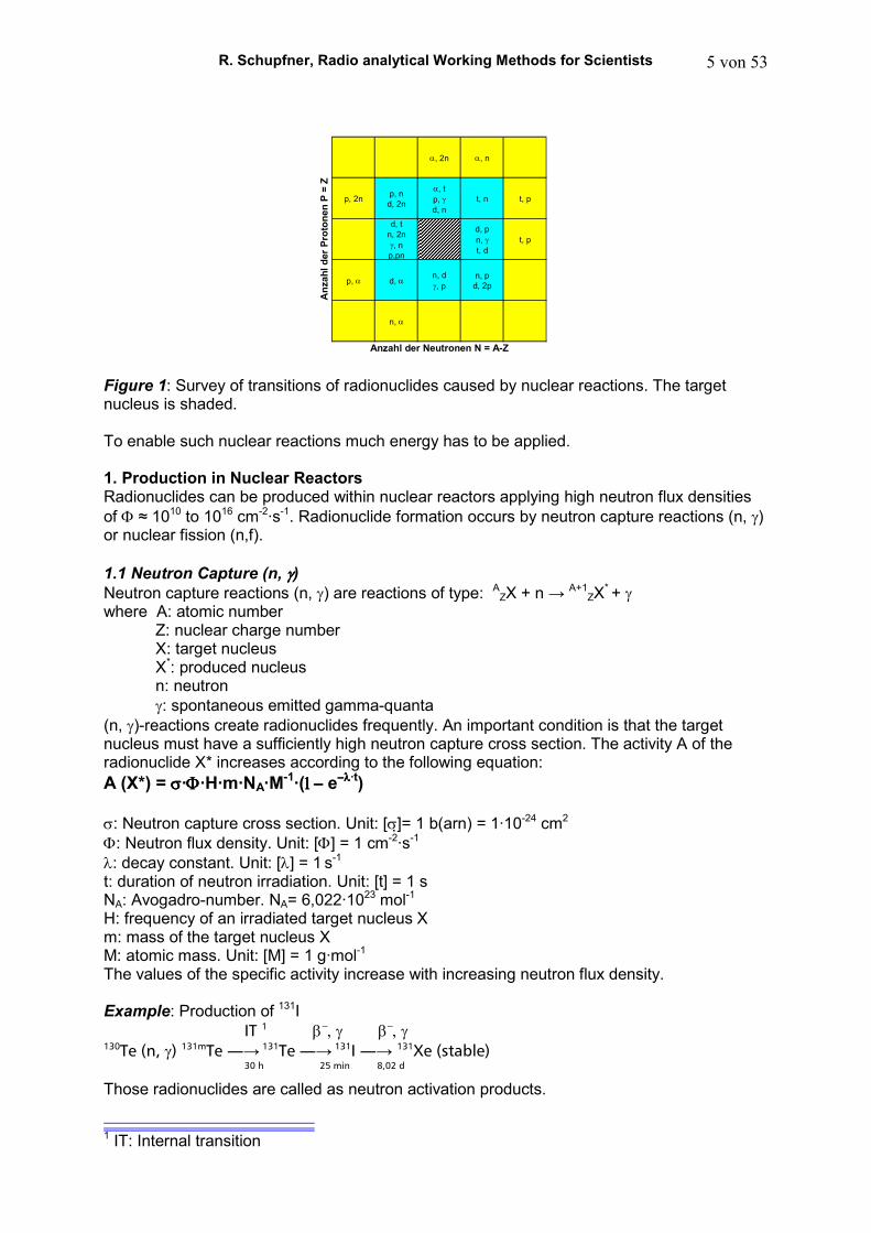
Figure 2: Nuclear energy scheme of 99Mo. As a rule MoO4
2- is fixed very strongly at high hydrated Al2O3. 99mTcO4- can be easily eluted
applying a physiological graded sodium chloride solution. β− IT β−
99Mo → 99mTc → 99Tc → 99Ru (stable) Y(99mTc) = 0,876
66,0 h 6,0 h 2,13·105 y β−
99Tc → 99Ru (stable) Y(99Tc) = 0,124
2,13·105 y 4. Labelled Compounds A number of organic and inorganic compounds are suited to be labelled with radionuclides at various positions of its molecular structure. For this purpose certain atoms have to be substituted by isotopic or even non isotopic radionuclides. There are a number of possibilities. For preparation the following parameters must be considered. Kind of radionuclides Labelling position concerning a certain position within the labelled molecule as well as all
atoms of a certain element. specific activity (activity related per mass unit of an element) chemical purity (portion of compound containing the wanted chemical species) radionuclide purity (portion of total radioactivity containing the specified radionuclide) radiochemical purity (portion of compound containing the wanted chemical species and
being bound to a specific positions within the molecule) The choice of parameters is depends on the application of the labelled compound. Labelled compounds may be produced by various reactions: Irradiation with protons of suited nitrogen containing targets e.g. 11CO und 11CO2. Chemical syntheses (applied at most frequently) Biochemical methods which enables the labelling of complex organic compounds. Exchange reactions to add radionuclides to inactive compounds. Backscatter- and radiation induced labelling Synthesis of labelled compounds requires the adherence to following rules: The masses of applied radionuclides are very small as a rule (below several mg). Methods are to be applied to assure a save handling, e.g. use of small compact vessels. To minimize waste as well as costs as far as possible effective reactions are to be
applied achieving high chemical yield. For routine syntheses automate procedures were developed to ensure a fast save and
reliable production of labelled compounds.
1/2 0,0
(1/2, 3/2ι 1,1418
3/2 1,0043/2 0,9206
0,6715
(1/2, 3/2ι 0,5091
5/2 0,1811
(1/2) 0,1426
(7/2) 0,1405 9/2 0,0
99Tc (2,13·10
5 y)
99Mo (66,0 h)
R. Schupfner, Radio analytical Working Methods for Scientists 8 von 53
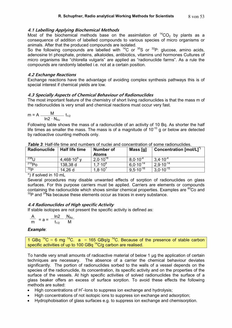
4.1 Labelling Applying Biochemical Methods Most of the biochemical methods base on the assimilation of 14CO2 by plants as a consequence of addition of labelled compounds to various species of micro organisms or animals. After that the produced compounds are isolated. So the following compounds are labelled with 14C or 35S or 32P: glucose, amino acids, adenosine tri phosphate, proteins, alkaloides, antibiotics, vitamins und hormones Cultures of micro organisms like “chlorella vulgaris” are applied as “radionuclide farms”. As a rule the compounds are randomly labelled i.e. not at a certain position. 4.2 Exchange Reactions Exchange reactions have the advantage of avoiding complex synthesis pathways this is of special interest if chemical yields are low. 4.3 Specially Aspects of Chemical Behaviour of Radionuclides The most important feature of the chemistry of short living radionuclides is that the mass m of the radionuclides is very small and chemical reactions must occur very fast. m = A t1/2 Following table shows the mass of a radionuclide of an activity of 10 Bq. As shorter the half life times as smaller the mass. The mass is of a magnitude of 10-10 g or below are detected by radioactive counting methods only. Table 3: Half-life time and numbers of nuclei and concentration of some radionuclides. Radionuclide Half life time Number of
Atoms Mass [g] Concentration [mol/L]*)
238U 4,468·109 y 2,0·1018 8,0·10-4 3,4·10-4 210Po 138,38 d 1,7·108 6,0·10-14 2,9·10-14 32P 14,26 d 1,8·107 9,5·10-16 3,0·10-15 *) if solved in 10 mL Several procedures may disable unwanted effects of sorption of radionuclides on glass surfaces. For this purpose carriers must be applied. Carriers are elements or compounds containing the radionuclide which shows similar chemical properties. Examples are 60Co and 32P and 24Na because these elements occur as traces in every substance. 4.4 Radionuclides of High specific Activity If stable isotopes are not present the specific activity is defined as: = a = Example: 1 GBq 14C ≈ 6 mg 14C. a ≈ 165 GBq/g 14C. Because of the presence of stable carbon specific activities of up to 100 GBq 14C/g carbon are realised. To handle very small amounts of radioactive material of below 1 µg the application of certain techniques are necessary. The absence of a carrier the chemical behaviour deviates significantly. The portion of radionuclides sorbed to the walls of a vessel depends on the species of the radionuclide, its concentration, its specific activity and on the properties of the surface of the vessels. At high specific activities of solved radionuclides the surface of a glass beaker offers an excess of surface sorption. To avoid these effects the following methods are suited: • High concentrations of H+-Ions to suppress ion exchange and hydrolysis; • High concentrations of not isotopic ions to suppress ion exchange and adsorption; • Hydrophobisation of glass surfaces e.g. to suppress ion exchange and chemisorption.
M ln2 · NAv
A m
ln2 t1/2
NAv M
R. Schupfner, Radio analytical Working Methods for Scientists 9 von 53
4.5 Radiocolloids
Radiocolloids are colloid species of very small amounts of radioactive substances. They can be separated from aqueous solutions applying ultra filtration, centrifugation and electrophoresis. They can easily be detected by autoradiography. Many organic molecules are big enough to form colloids. Therefore organic colloids are often applied to life sciences. 4.6 Trace Techniques Trace techniques enclose all methods adding very small amounts (traces) of radionuclides or labelled compounds to study the behaviour or the transport or the chemical reaction of an element or compound of interest within this system. Radioactive tracers are very suited because they can be detected sensitively. Example: At a counting time of 10 minutes and a counting efficiency of 20 % an activity of 10 Becquerel (Bq) can be detected with a statistic uncertainty of about 3 % only. The basic condition to apply tracer techniques is that the applied radionuclide must adopt the same chemical species as the species to be studied. As a rule this can be considered as true applying isotopic tracers as far as isotopic effects are excluded.
C. Radioactivity
1. Stability of the Atomic Nucleus
At 1896 Henri Becquerel described the phenomena of radioactivity causing blackening of films by uranium containing minerals. Two years later Pierre and Marie Curie discovered further radioactive elements of the uranium decay chain. The new found elements were present only in very small amounts and could be detected only by the emitted ionizing radiation. Soddy suggested using the term of isotope in1913. Isotopes are species of atoms differing only in its mass number. A further important term to characterise atomic species due to its charge or mass numbers is nuclide. Atomic nuclei consist of neutrons and protons which are known as nucleons. Nucleons are combined by nuclear forces (strong forces). Nuclides are different species of atomic nuclei which differ in nuclear charge number Z and atomic mass number A and nuclear energy state.
The notation according to IUPAC is: A(element symbol) or (element symbol)-A
Radionuclides are unstable species of atoms decaying to other nuclides emitting ionising radiation. To characterize radionuclides data of the energy and emission probability of ionising radiation are necessary. At present there 104 different elements are known including about 1300 nuclides. 270 of them are stable. The stability of an atomic nucleus can be explained by the droplet model (Bethe-Weizäcker-formula).
2. Principles of the Radioactive Decay 2.1 Activity versus Time
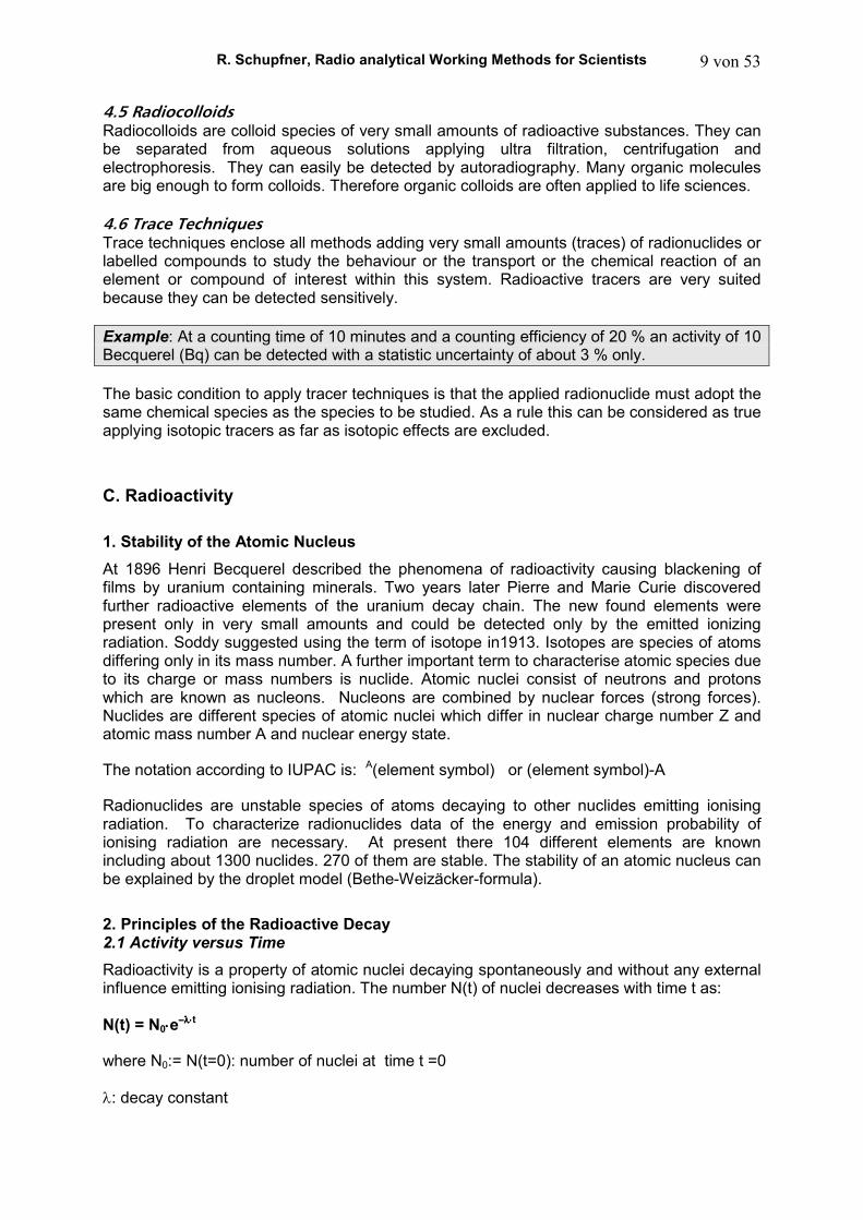
Radioactivity is a property of atomic nuclei decaying spontaneously and without any external influence emitting ionising radiation. The number N(t) of nuclei decreases with time t as:
N(t) = N0⋅⋅⋅⋅e−λ−λ−λ−λ⋅⋅⋅⋅t
where N0:= N(t=0): number of nuclei at time t =0
λ: decay constant
R. Schupfner, Radio analytical Working Methods for Scientists 10 von 53
The activity A is defined as
A = = λ·N
Depending on time t according to following equation:
A(t) = A0⋅⋅⋅⋅e−λ−λ−λ−λ⋅⋅⋅⋅t
A0:=A(t=0): Activity at time t=0.
The half life time t1/2 is a fundamental universal constant characterising each radionuclide unambiguously. Its value can not be affected by any means. Relation between decay constant λ and half life time t1/2 is geven by the following equation:
t1/2= ln(2)/λ
There are used several units:
[A] = 1 Bq (Becquerel) = 1 decay per second [A] = 1dpm = 1 decay per minute = 1/60 Bq [A] = 1 Ci (Currie) = 3,7·1010 Bq
After one single half life time t1/2 one half of the observed numbers of nuclei of every radionuclide has decayed. The value of half life time ranges from µs more than 1021 years (76Ge). An old fashioned term is the mean life time τ being defined as:
τ := λ-1
After a time period of τ the activity of a radionuclide decreases to the reciprocal of Euler´s number e-1 ≈ 0,37 compared to the value at the beginning of observation (t =0) .
Exercises: a) A sample contains a activity of 2,7 MBq. Which value is it in Ci ? The result of the detection of activity is 99400 dpm. Convert this value to Bq and Ci. Use suited abbreviation such as µ = 10-6, m = 10-3, k = 103, M = 106.
b) Calculate the activity of a radionuclide after 5 t1/2 and after 10 t1/2
c) DNA is labelled with A1 = 10 mCi of 32P (t1/2 = 14,2 d) and A2 = 100 µCi of 125I(t1/2 = 60,5 d). In your laboratory it is allowed to handle the 10 fold of the activity limits AL according to the sum formula:
+ < 10
How long must you wait, if you want to use this labelled DNA in your laboratory?
AL1 32P: 1 MBq , AL2 = 10 kBq
number dN of decaying nuclides time interval dt
A1
AL1
A2
AL2
R. Schupfner, Radio analytical Working Methods for Scientists 11 von 53
Figure 3: Activity versus time if radioactive decay law.
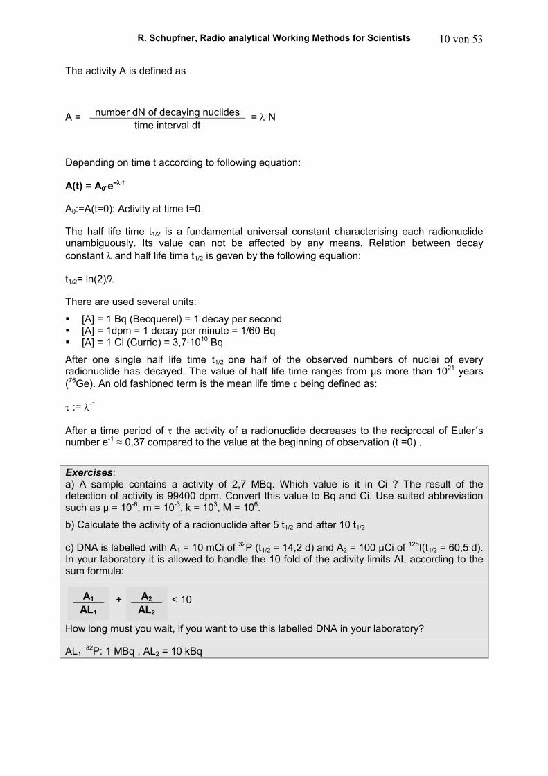
2.2 Statistics of Radioactive Decay The frequency zn = λ⋅∆t that the number of n decays occur within a time period of ∆t a is independent of time t and is approximately described by a Poisson distribution.
Where
Z: number of total decays observed ν: mean value of the number of decays
With Z =100 and ν = 5, 10, 15, 20 the following curves are received.
0
2
4
6
8
10
12
14
16
18
20
0 5 10 15 20 25 30 35
n
zn
5 10 15 20ν =
Figure 4: Frequency zn = λ⋅∆t of decays versus number of decays n within ∆t at various mean values ν.
R. Schupfner, Radio analytical Working Methods for Scientists 12 von 53
The standard deviation ∆n of mean decays ν is: ∆n = √ν
At increasing numbers of mean decays ν the Poisson distribution shades into a Gaussian distribution. 2.3 Activity and Mass
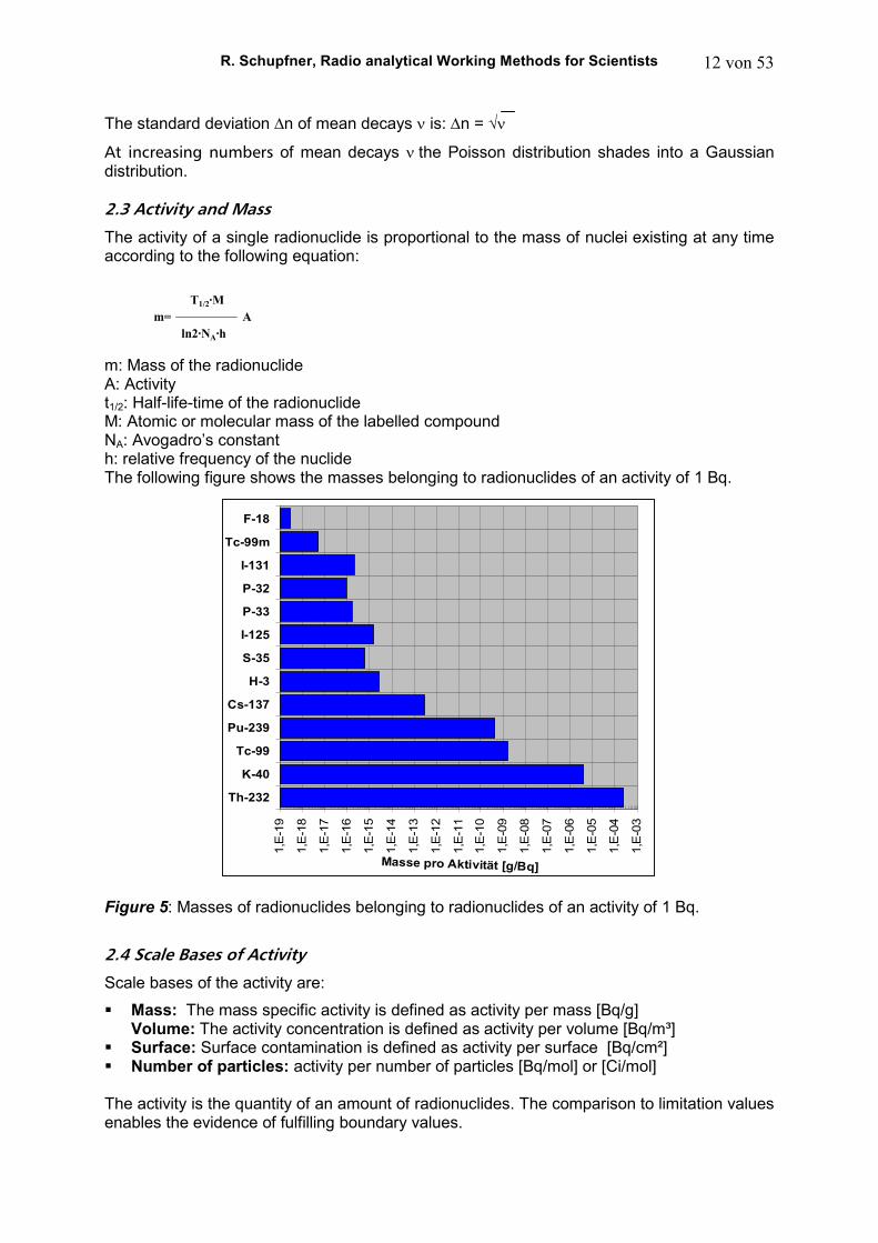
The activity of a single radionuclide is proportional to the mass of nuclei existing at any time according to the following equation:
m: Mass of the radionuclide A: Activity t1/2: Half-life-time of the radionuclide M: Atomic or molecular mass of the labelled compound NA: Avogadro’s constant h: relative frequency of the nuclide The following figure shows the masses belonging to radionuclides of an activity of 1 Bq.
1,E
-19
1,E
-18
1,E
-17
1,E
-16
1,E
-15
1,E
-14
1,E
-13
1,E
-12
1,E
-11
1,E
-10
1,E
-09
1,E
-08
1,E
-07
1,E
-06
1,E
-05
1,E
-04
1,E
-03
Th-232
K-40
Tc-99
Pu-239
Cs-137
H-3
S-35
I-125
P-33
P-32
I-131
Tc-99m
F-18
Masse pro Aktivität [g/Bq]
Figure 5: Masses of radionuclides belonging to radionuclides of an activity of 1 Bq.
2.4 Scale Bases of Activity
Scale bases of the activity are:
Mass: The mass specific activity is defined as activity per mass [Bq/g] Volume: The activity concentration is defined as activity per volume [Bq/m³]
Surface: Surface contamination is defined as activity per surface [Bq/cm²] Number of particles: activity per number of particles [Bq/mol] or [Ci/mol]
The activity is the quantity of an amount of radionuclides. The comparison to limitation values enables the evidence of fulfilling boundary values.
T1/2·M
m= A
ln2·NA·h
R. Schupfner, Radio analytical Working Methods for Scientists 13 von 53
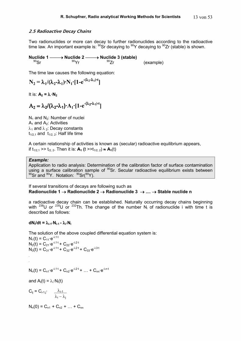
2.5 Radioactive Decay Chains Two radionuclides or more can decay to further radionuclides according to the radioactive time law. An important example is: 90Sr decaying to 90Y decaying to 90Zr (stable) is shown.
Nuclide 1 →→→→ Nuclide 2 →→→→ Nuclide 3 (stable) 90Sr 90Yr 90Zr (example) The time law causes the following equation:
It is: A2 = λλλλ⋅⋅⋅⋅·N2
N1 and N2: Number of nuclei A1 and A2: Activities λ1 and λ 2: Decay constants t1/2,1 and t1/2, 2: Half life time A certain relationship of activities is known as (secular) radioactive equilibrium appears, if t1/2,1 >> t/2, 2. Then it is: A1 (t >>t1/2, 2) ≈≈≈≈ A1(t) Example: Application to radio analysis: Determination of the calibration factor of surface contamination using a surface calibration sample of 90Sr. Secular radioactive equilibrium exists between 90Sr and 90Y. Notation: 90Sr(90Y). If several transitions of decays are following such as Radionuclide 1 →→→→ Radionuclide 2 →→→→ Radionuclide 3 →→→→ .... →→→→ Stable nuclide n a radioactive decay chain can be established. Naturally occurring decay chains beginning with 238U or 235U or 232Th. The change of the number Ni of radionuclide i with time t is described as follows:
dNi/dt = λλλλi-1⋅⋅⋅⋅Ni-1 - λλλλi⋅⋅⋅⋅Ni
The solution of the above coupled differential equation system is: N1(t) = C11·e-λ1·t
N2(t) = C21·e-λ1·t + C22·e-λ2·t
N3(t) = C31·e-λ1·t + C32·e-λ2·t + C33·e-λ3·t
.
.
Nn(t) = Cn1·e-λ1·t + Cn2·e-λ2·t + … + Cnn·e-λn·t
and Ai(t) = λi·Ni(t) Cij = Ci-1,j·
Nn(0) = Cn1
+ Cn2 + … + Cnn
N2 = λλλλ1/(λλλλ2-λλλλ1)·N1·[1-e-(λλλλ2-λλλλ1)·t
]
ΑΑΑΑ2222 = λ = λ = λ = λ2/(λλλλ2-λλλλ1)·A1·[1-e-(λλλλ2-λλλλ1)·t
]
λi-1 λi − λj
R. Schupfner, Radio analytical Working Methods for Scientists 14 von 53
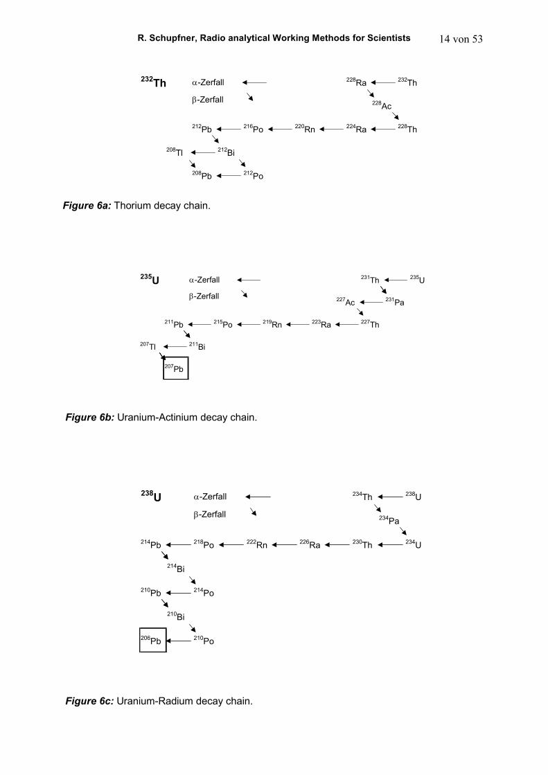
Figure 6b: Uranium-Actinium decay chain.
Figure 6c: Uranium-Radium decay chain.
232Th α-Zerfall 228Ra 232Th
β-Zerfall 228Ac
212Pb 216Po 220Rn 224Ra 228Th
208Tl 212Bi
208Pb 212Po
235U α-Zerfall 231Th 235U
β-Zerfall 227Ac 231Pa
211Pb 215Po 219Rn 223Ra 227Th
207Tl 211Bi
207Pb
Figure 6a: Thorium decay chain.
238U α-Zerfall 234Th 238U
β-Zerfall 234Pa
214Pb 218Po 222Rn 226Ra 230Th 234U
214Bi
210Pb 214Po
210Bi
206Pb 210Po
R. Schupfner, Radio analytical Working Methods for Scientists 15 von 53
3. Modes of Decay and Nuclear Radiation
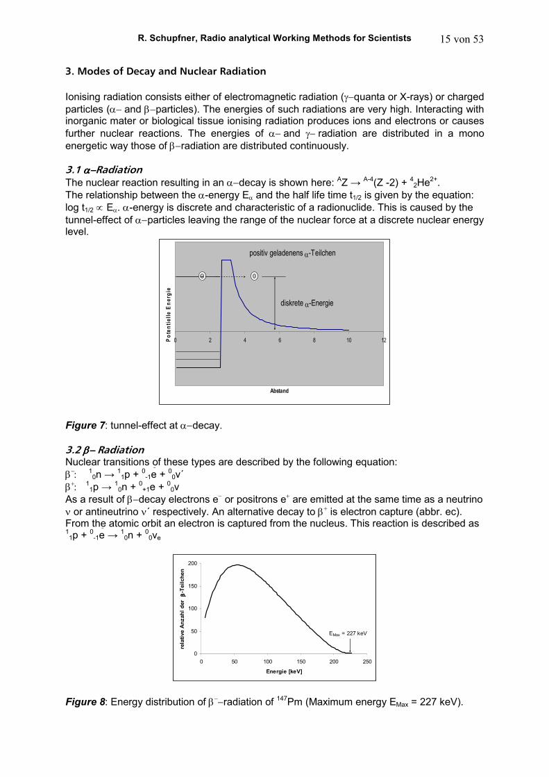
Ionising radiation consists either of electromagnetic radiation (γ−quanta or X-rays) or charged particles (α− and β−particles). The energies of such radiations are very high. Interacting with inorganic mater or biological tissue ionising radiation produces ions and electrons or causes further nuclear reactions. The energies of α− and γ− radiation are distributed in a mono energetic way those of β−radiation are distributed continuously. 3.1 α−α−α−α−Radiation The nuclear reaction resulting in an α−decay is shown here: AZ → A-4(Z -2) + 42He2+. The relationship between the α-energy Eα and the half life time t1/2 is given by the equation: log t1/2 ∝ Eα. α-energy is discrete and characteristic of a radionuclide. This is caused by the tunnel-effect of α−particles leaving the range of the nuclear force at a discrete nuclear energy level.
0 2 4 6 8 10 12
Abstand
Po
ten
tie
lle
En
erg
ie
positiv geladenens α-Teilchen
diskrete α-Energie
Figure 7: tunnel-effect at α−decay. 3.2 β− β− β− β− Radiation Nuclear transitions of these types are described by the following equation: β
−: 10n → 11p + 0-1e + 00ν´
β+: 11p → 10n + 0+1e + 00ν
As a result of β−decay electrons e− or positrons e+ are emitted at the same time as a neutrino ν or antineutrino ν´ respectively. An alternative decay to β+ is electron capture (abbr. ec). From the atomic orbit an electron is captured from the nucleus. This reaction is described as 11p + 0-1e → 10n + 00νe
0
50
100
150
200
0 50 100 150 200 250
Energie [keV]
rela
tive A
nzah
l d
er
ββ ββ-T
eil
ch
en
EMax = 227 keV
Figure 8: Energy distribution of β−
−radiation of 147Pm (Maximum energy EMax = 227 keV).
R. Schupfner, Radio analytical Working Methods for Scientists 16 von 53
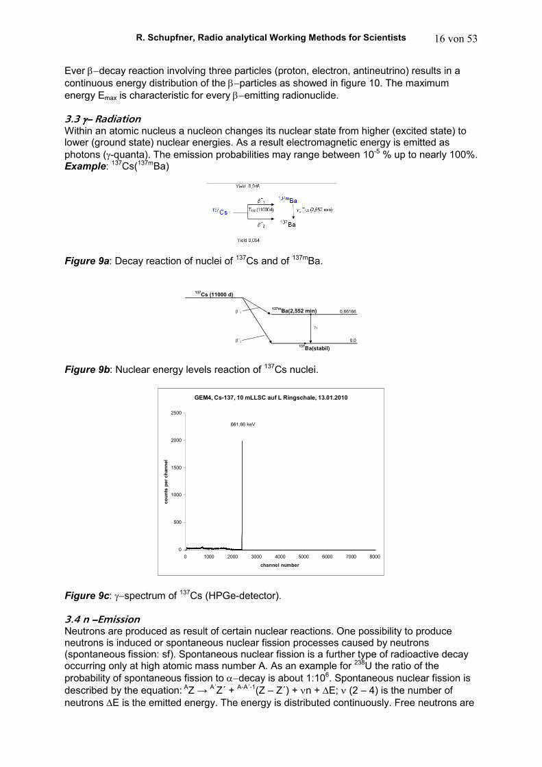
Ever β−decay reaction involving three particles (proton, electron, antineutrino) results in a continuous energy distribution of the β−particles as showed in figure 10. The maximum energy Emax is characteristic for every β−emitting radionuclide. 3.3 γ− γ− γ− γ− Radiation Within an atomic nucleus a nucleon changes its nuclear state from higher (excited state) to lower (ground state) nuclear energies. As a result electromagnetic energy is emitted as photons (γ-quanta). The emission probabilities may range between 10-5 % up to nearly 100%. Example: 137Cs(137mBa)
Figure 9a: Decay reaction of nuclei of 137Cs and of 137mBa.
β−
1
137mBa(2,552 min) 0,66166
β−
2 0,0
137Cs (11000 d)
137Ba(stabil)
γ1
Figure 9b: Nuclear energy levels reaction of 137Cs nuclei.
GEM4, Cs-137, 10 mLLSC auf L Ringschale, 13.01.2010
0
500
1000
1500
2000
2500
0 1000 2000 3000 4000 5000 6000 7000 8000
channel number
co
un
ts p
er
ch
an
nel
661,66 keV
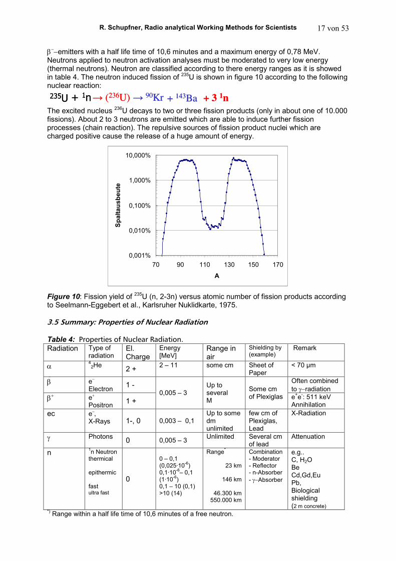
Figure 9c: γ−spectrum of 137Cs (HPGe-detector). 3.4 n −−−−Emission Neutrons are produced as result of certain nuclear reactions. One possibility to produce neutrons is induced or spontaneous nuclear fission processes caused by neutrons (spontaneous fission: sf). Spontaneous nuclear fission is a further type of radioactive decay occurring only at high atomic mass number A. As an example for 238U the ratio of the probability of spontaneous fission to α−decay is about 1:106. Spontaneous nuclear fission is described by the equation: AZ → A´Z´ + A-A´-1(Z – Z´) + νn + ∆E; ν (2 – 4) is the number of neutrons ∆E is the emitted energy. The energy is distributed continuously. Free neutrons are
R. Schupfner, Radio analytical Working Methods for Scientists 17 von 53
β−−emitters with a half life time of 10,6 minutes and a maximum energy of 0,78 MeV.
Neutrons applied to neutron activation analyses must be moderated to very low energy (thermal neutrons). Neutron are classified according to there energy ranges as it is showed in table 4. The neutron induced fission of 235U is shown in figure 10 according to the following nuclear reaction: The excited nucleus 236U decays to two or three fission products (only in about one of 10.000 fissions). About 2 to 3 neutrons are emitted which are able to induce further fission processes (chain reaction). The repulsive sources of fission product nuclei which are charged positive cause the release of a huge amount of energy.
0,001%
0,010%
0,100%
1,000%
10,000%
70 90 110 130 150 170
A
Sp
alt
au
sb
eu
te
Figure 10: Fission yield of 235U (n, 2-3n) versus atomic number of fission products according to Seelmann-Eggebert et al., Karlsruher Nuklidkarte, 1975. 3.5 Summary: Properties of Nuclear Radiation Table 4: Properties of Nuclear Radiation. Radiation Type of
radiation El. Charge
Energy [MeV]
Range in air
Shielding by (example)
Remark
α 42He 2 + 2 – 11 some cm Sheet of
Paper < 70 µm
β e−
Electron 1 - Often combined
to γ−radiation β
+ e+
Positron 1 + 0,005 – 3
Up to several M
Some cm of Plexiglas e+e-: 511 keV
Annihilation ec e−
,
X-Rays 1-, 0 0,003 – 0,1 Up to some dm unlimited
few cm of Plexiglas, Lead
X-Radiation
γ Photons 0 0,005 – 3 Unlimited Several cm of lead
Attenuation
n 1n Neutron thermical epithermic fast ultra fast
0
0 – 0,1 (0,025·10-6) 0,1·10-6– 0,1 (1·10-6) 0,1 – 10 (0,1) >10 (14)
Range*
23 km
146 km
46.300 km
550.000 km
Combination - Moderator - Reflector - n-Absorber - γ−Absorber
e.g.. C, H2O Be Cd,Gd,Eu Pb, Biological shielding (2 m concrete)
*) Range within a half life time of 10,6 minutes of a free neutron.
235U + 1n → (236U) → 90Kr + 143Ba + 3 1n235U + 1n → (236U) → 90Kr + 143Ba + 3 1n
R. Schupfner, Radio analytical Working Methods for Scientists 18 von 53
D. Radiation Exposure
1. Harmful Effects of Ionizing Radiation on the Human Body The effects of ionising radiation to the human body are called radiation exposure. Depending on the site of a radiation source is situated either inside or outside of the body an internal or external radiation exposure is caused. γ−emitter may cause both. The high amount of energy of ionising radiation removes electrons from the atoms of bio molecules and therefore causes a chemical change. This energy dissipation causes the harmful effects of ionizing radiation which are shown schematically in the following figure:
no detectable harmdeath
deteterminstical effects statistical effects
cancer, malformation
incomplete complete
repare mechanisms
deathat high dose vallues of some Sv
no detectable harmat low dose values below 0,4 Sv
death of cell
Transfer of radiation energy to atoms and molecules
change of the structure of biomolecules
Formation of toxic compounds (e.g. radicals or cell poisons)
change of the metabloism of cells
Figure 11: The harmful effects of ionising radiation.
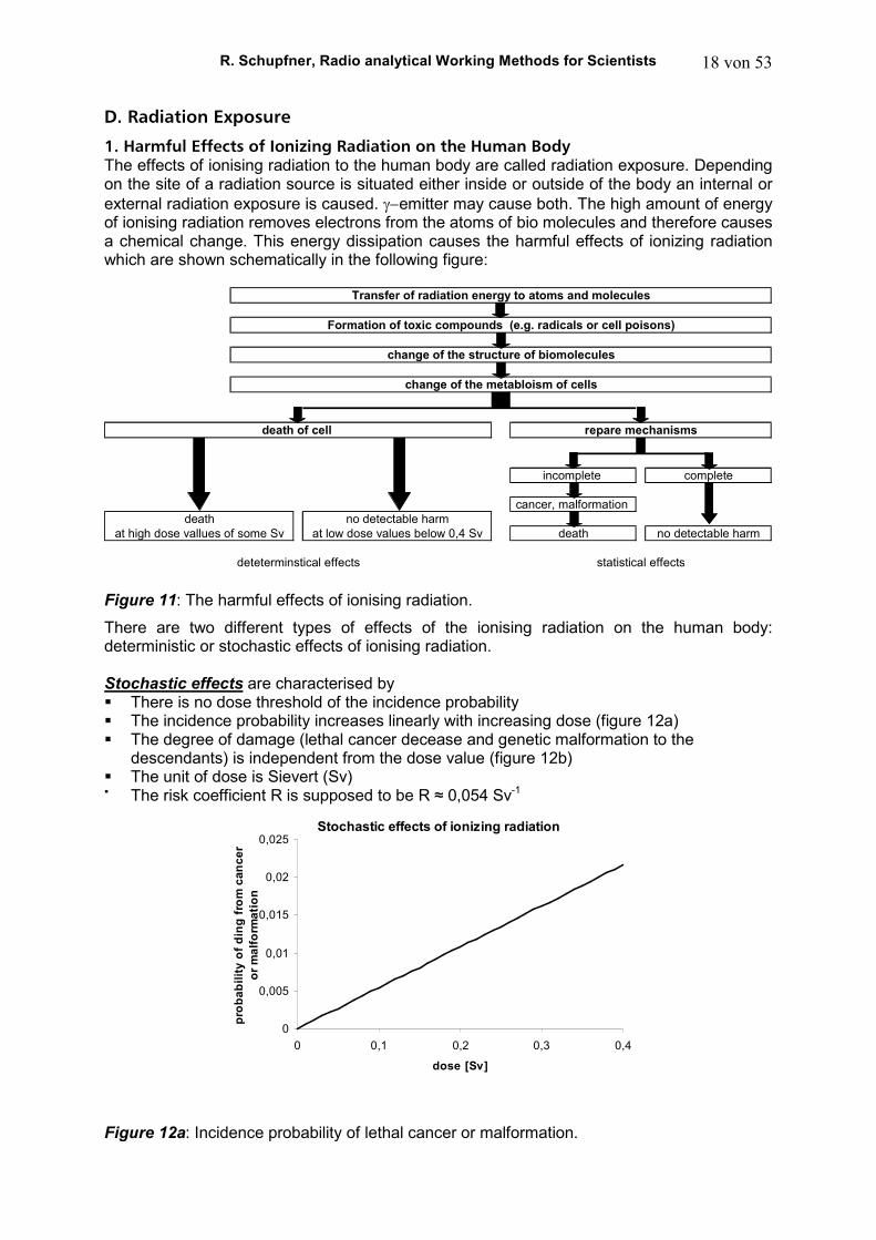
There are two different types of effects of the ionising radiation on the human body: deterministic or stochastic effects of ionising radiation. Stochastic effects are characterised by There is no dose threshold of the incidence probability The incidence probability increases linearly with increasing dose (figure 12a) The degree of damage (lethal cancer decease and genetic malformation to the
descendants) is independent from the dose value (figure 12b) The unit of dose is Sievert (Sv) The risk coefficient R is supposed to be R ≈ 0,054 Sv-1
Stochastic effects of ionizing radiation
0
0,005
0,01
0,015
0,02
0,025
0 0,1 0,2 0,3 0,4
dose [Sv]
pro
ba
bil
ity
of
din
g f
rom
ca
nc
er
or
ma
lfo
rma
tio
n
Figure 12a: Incidence probability of lethal cancer or malformation.
R. Schupfner, Radio analytical Working Methods for Scientists 19 von 53
Stochastic effects of ionizing radiation
0
0,1
0,2
0,3
0,4
0,5
0,6
0,7
0,8
0,9
1
0 1 2 3 4 5 6
dose [Sv]
degree of damage
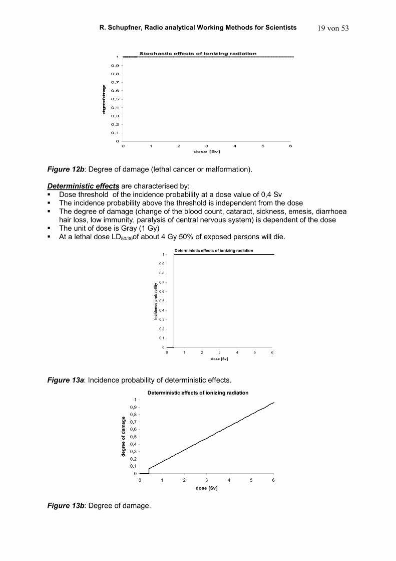
Figure 12b: Degree of damage (lethal cancer or malformation). Deterministic effects are characterised by: Dose threshold of the incidence probability at a dose value of 0,4 Sv The incidence probability above the threshold is independent from the dose The degree of damage (change of the blood count, cataract, sickness, emesis, diarrhoea
hair loss, low immunity, paralysis of central nervous system) is dependent of the dose The unit of dose is Gray (1 Gy) At a lethal dose LD50/30of about 4 Gy 50% of exposed persons will die. Figure 13a: Incidence probability of deterministic effects.
Deterministic effects of ionizing radiation
0
0,1
0,2
0,3
0,4
0,5
0,6
0,7
0,8
0,9
1
0 1 2 3 4 5 6
dose [Sv]
de
gre
e o
f d
am
ag
e
Figure 13b: Degree of damage.
Deterministic effects of ionizing radiation
0
0,1
0,2
0,3
0,4
0,5
0,6
0,7
0,8
0,9
1
0 1 2 3 4 5 6
dose [Sv]
inc
ide
nc
e p
rob
ab
ilit
y
R. Schupfner, Radio analytical Working Methods for Scientists 20 von 53
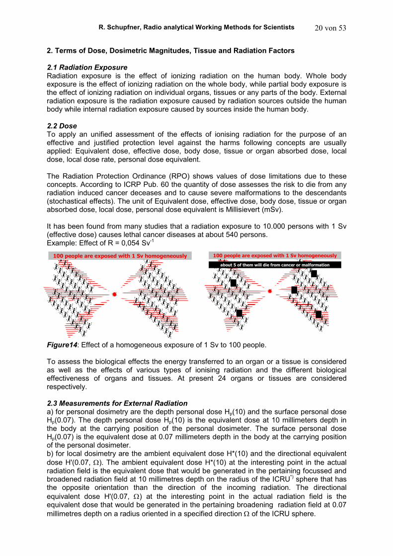
2. Terms of Dose, Dosimetric Magnitudes, Tissue and Radiation Factors 2.1 Radiation Exposure Radiation exposure is the effect of ionizing radiation on the human body. Whole body exposure is the effect of ionizing radiation on the whole body, while partial body exposure is the effect of ionizing radiation on individual organs, tissues or any parts of the body. External radiation exposure is the radiation exposure caused by radiation sources outside the human body while internal radiation exposure caused by sources inside the human body. 2.2 Dose To apply an unified assessment of the effects of ionising radiation for the purpose of an effective and justified protection level against the harms following concepts are usually applied: Equivalent dose, effective dose, body dose, tissue or organ absorbed dose, local dose, local dose rate, personal dose equivalent. The Radiation Protection Ordinance (RPO) shows values of dose limitations due to these concepts. According to ICRP Pub. 60 the quantity of dose assesses the risk to die from any radiation induced cancer deceases and to cause severe malformations to the descendants (stochastical effects). The unit of Equivalent dose, effective dose, body dose, tissue or organ absorbed dose, local dose, personal dose equivalent is Millisievert (mSv). It has been found from many studies that a radiation exposure to 10.000 persons with 1 Sv (effective dose) causes lethal cancer diseases at about 540 persons. Example: Effect of R = 0,054 Sv-1
Figure14: Effect of a homogeneous exposure of 1 Sv to 100 people. To assess the biological effects the energy transferred to an organ or a tissue is considered as well as the effects of various types of ionising radiation and the different biological effectiveness of organs and tissues. At present 24 organs or tissues are considered respectively. 2.3 Measurements for External Radiation a) for personal dosimetry are the depth personal dose Hp(10) and the surface personal dose Hp(0.07). The depth personal dose Hp(10) is the equivalent dose at 10 millimeters depth in the body at the carrying position of the personal dosimeter. The surface personal dose Hp(0.07) is the equivalent dose at 0.07 millimeters depth in the body at the carrying position of the personal dosimeter. b) for local dosimetry are the ambient equivalent dose H*(10) and the directional equivalent dose H'(0.07, Ω). The ambient equivalent dose H*(10) at the interesting point in the actual radiation field is the equivalent dose that would be generated in the pertaining focussed and broadened radiation field at 10 millimetres depth on the radius of the ICRU*) sphere that has the opposite orientation than the direction of the incoming radiation. The directional equivalent dose H'(0.07, Ω) at the interesting point in the actual radiation field is the equivalent dose that would be generated in the pertaining broadening radiation field at 0.07 millimetres depth on a radius oriented in a specified direction Ω of the ICRU sphere.
100 people are exposed with 1 Sv homogeneously 100 people are exposed with 1 Sv homogeneously
about 5 of them will die from cancer or malformation
R. Schupfner, Radio analytical Working Methods for Scientists 21 von 53
In this context: - a broadened radiation field is an idealized radiation field where the particle flow density
and the energy and direction spread of the radiation at all points of a sufficiently large volume show the same levels as the actual radiation field at the interesting point.
- a broadened and focused field is an idealized radiation that is broadened and, in addition, in which the radiation is focused in one direction,
- the ICRU sphere constitutes a spherical phantom of 30 centimetres diameter of ICRU*) soft tissue (tissue-equivalent material of the density 1 g/cm³, composition: 76,2 % oxygen, 11,1% carbon, 10,1% hydrogen, 2,6% nitrogen)
The unit of the equivalent dose is the sievert (unit abbreviation Sv). 2.4 Calculation of the Body Dose 2.4.1 Calculation of the organ absorbed dose equivalent HT The organ absorbed dose HT,R is the product of the energy dose averaged though the tissue T, the organ energy dose DT,R generated through the radiation R and the radiation weighting factor wR in the accordance with table 5 HT,R = wR· DT,R If the radiation consists of types and energies with different values of wR, the individual amounts shall be added together. The following shall then apply to the total organ absorbed dose HT:
HT = ΣwR· DT,R R
The unit of the organ absorbed dose equivalent is the sievert (unit abbreviation Sv). In praxis often mSv = 0,001 Sv or µSv = 0,000.001 Sv is used.
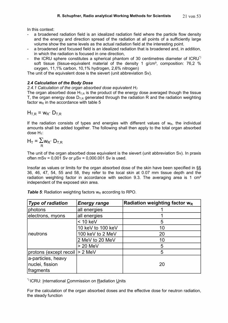
Insofar as values or limits for the organ absorbed dose of the skin have been specified in §§ 36, 46, 47, 54, 55 and 58, they refer to the local skin at 0.07 mm tissue depth and the radiation weighting factor in accordance with section 9.3. The averaging area is 1 cm² independent of the exposed skin area. Table 5: Radiation weighting factors wR according to RPO. Type of radiation Energy range Radiation weighting factor wR
photons all energies 1electrons, myons all energies 1
< 10 keV 510 keV to 100 keV 10100 keV to 2 MeV 202 MeV to 20 MeV 10> 20 MeV 5
protons (except recoil protons)> 2 MeV 5a-particles, heavy nuclei, fission fragments
20
neutrons
*) ICRU: International Commission on Radiation Units For the calculation of the organ absorbed doses and the effective dose for neutron radiation, the steady function
R. Schupfner, Radio analytical Working Methods for Scientists 22 von 53
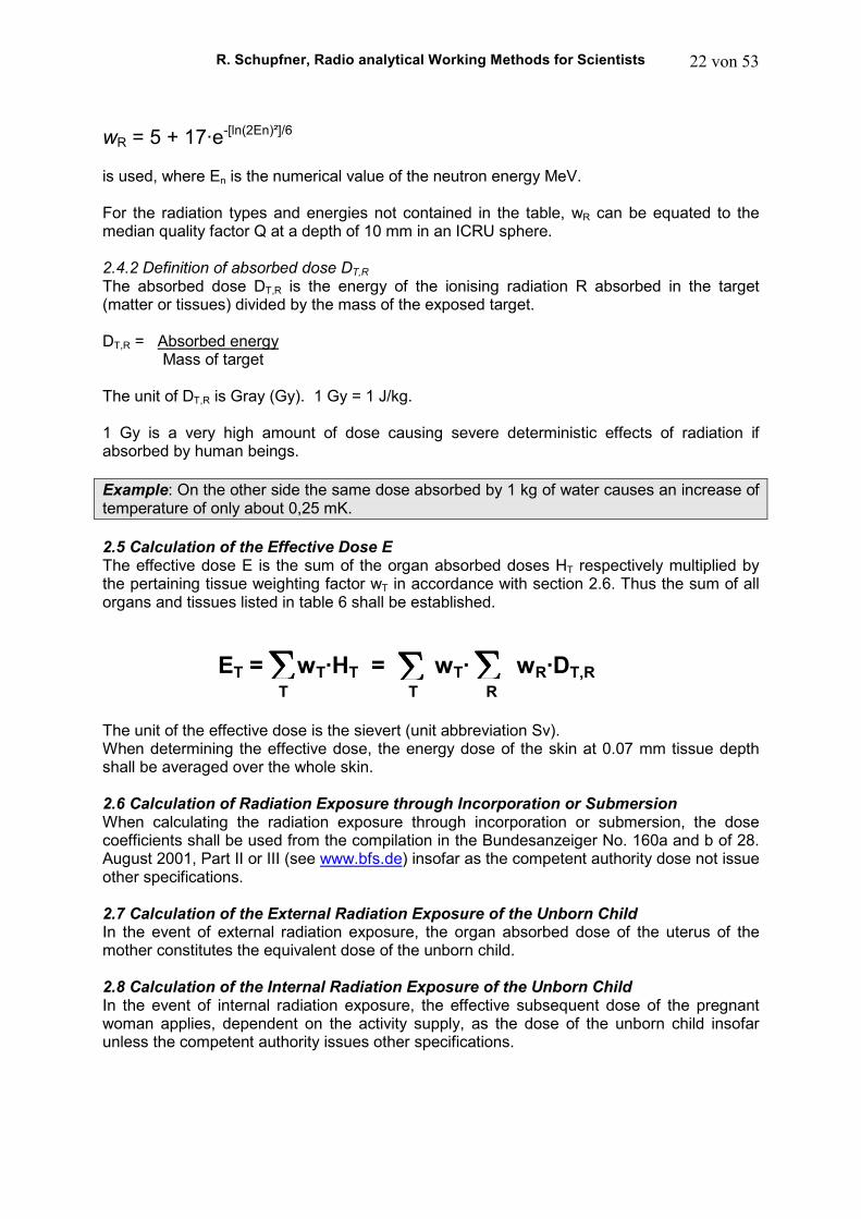
wR = 5 + 17·e-[ln(2En)²]/6 is used, where En is the numerical value of the neutron energy MeV. For the radiation types and energies not contained in the table, wR can be equated to the median quality factor Q at a depth of 10 mm in an ICRU sphere. 2.4.2 Definition of absorbed dose DT,R The absorbed dose DT,R is the energy of the ionising radiation R absorbed in the target (matter or tissues) divided by the mass of the exposed target. DT,R = Absorbed energy Mass of target The unit of DT,R is Gray (Gy). 1 Gy = 1 J/kg. 1 Gy is a very high amount of dose causing severe deterministic effects of radiation if absorbed by human beings. Example: On the other side the same dose absorbed by 1 kg of water causes an increase of temperature of only about 0,25 mK. 2.5 Calculation of the Effective Dose E The effective dose E is the sum of the organ absorbed doses HT respectively multiplied by the pertaining tissue weighting factor wT in accordance with section 2.6. Thus the sum of all organs and tissues listed in table 6 shall be established.
ET = wT·HT = wT· wR·DT,R
T T RΣΣΣΣ ΣΣΣΣ ΣΣΣΣ
The unit of the effective dose is the sievert (unit abbreviation Sv). When determining the effective dose, the energy dose of the skin at 0.07 mm tissue depth shall be averaged over the whole skin. 2.6 Calculation of Radiation Exposure through Incorporation or Submersion When calculating the radiation exposure through incorporation or submersion, the dose coefficients shall be used from the compilation in the Bundesanzeiger No. 160a and b of 28. August 2001, Part II or III (see www.bfs.de) insofar as the competent authority dose not issue other specifications. 2.7 Calculation of the External Radiation Exposure of the Unborn Child In the event of external radiation exposure, the organ absorbed dose of the uterus of the mother constitutes the equivalent dose of the unborn child. 2.8 Calculation of the Internal Radiation Exposure of the Unborn Child In the event of internal radiation exposure, the effective subsequent dose of the pregnant woman applies, dependent on the activity supply, as the dose of the unborn child insofar unless the competent authority issues other specifications.
R. Schupfner, Radio analytical Working Methods for Scientists 23 von 53
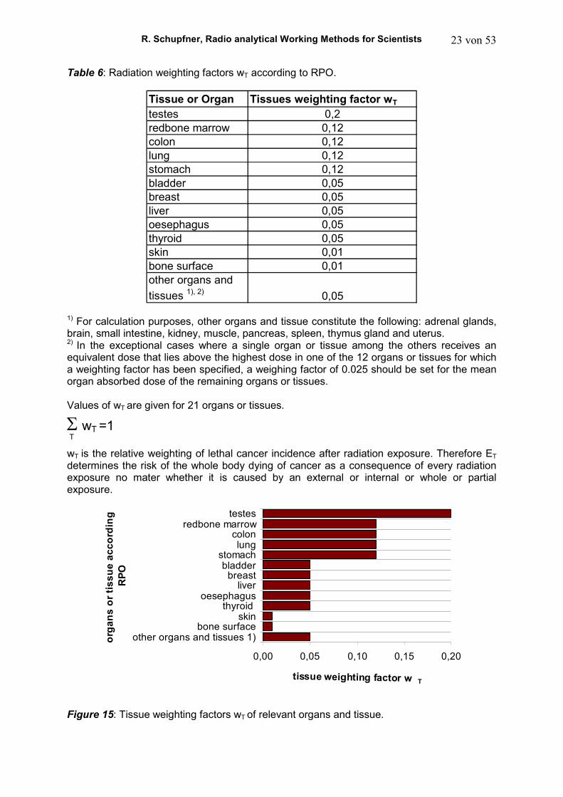
Table 6: Radiation weighting factors wT according to RPO.
Tissue or Organ Tissues weighting factor wT
testes 0,2redbone marrow 0,12colon 0,12lung 0,12stomach 0,12bladder 0,05breast 0,05liver 0,05oesephagus 0,05thyroid 0,05skin 0,01bone surface 0,01other organs and tissues 1), 2) 0,05
1) For calculation purposes, other organs and tissue constitute the following: adrenal glands, brain, small intestine, kidney, muscle, pancreas, spleen, thymus gland and uterus. 2) In the exceptional cases where a single organ or tissue among the others receives an equivalent dose that lies above the highest dose in one of the 12 organs or tissues for which a weighting factor has been specified, a weighing factor of 0.025 should be set for the mean organ absorbed dose of the remaining organs or tissues. Values of wT are given for 21 organs or tissues.
Σ wT =1 T
wT is the relative weighting of lethal cancer incidence after radiation exposure. Therefore ET determines the risk of the whole body dying of cancer as a consequence of every radiation exposure no mater whether it is caused by an external or internal or whole or partial exposure.
0,00 0,05 0,10 0,15 0,20
testesredbone marrow
colonlung
stomachbladder
breastliver
oesephagusthyroid
skinbone surface
other organs and tissues 1)org
an
s o
r ti
ss
ue
ac
co
rdin
g
RP
O
tissue weighting factor w T
Figure 15: Tissue weighting factors wT of relevant organs and tissue.
R. Schupfner, Radio analytical Working Methods for Scientists 24 von 53
Example: Practise with 32P labelled causes an equivalent dose Hskin = 22 mSv to the skin of the right hand and of Hlung = 4 mSv to the lungs. Determine the effective dose ET. ET = wlung· Hlung + wskin· Hskin = 0,12·4 mSv + 0,01·22 mSv = 0,48 mSv + 0,22 mSv = 0,70 mSv 2.9 Local Dose HL The local dose is given by the equivalent dose measured at a given location by means of the quantity to be measured as specified in Appendix VI, Part A. 2.10 Local Dose Rate ĤL The local dose rate is given by the local dose generated in a given time interval, divided by the length of that time interval. The unity is µSv/h. The mean local dose rate in Germany is below 0,1 µSv/h. 2.11 Calculation of the Organ Committed Dose HT(ττττ) and the Effective Committed Dose E (ττττ)
2.11.1 Calculation of the organ committed dose HT(τ)
The organ committed dose HT(τ) is the time integral of the organ absorbed dose rate in the tissue or organ T which a person receives because of an incorporation of radioactive substances:
HT(ττττ) = HT(t) dt.
t0
t0 + τ
for an incorporation at the time t0 with
.
HT(t) median organ absorbed doe rate in the tissue or organ T at the time t τ period of time specified in years over which integration takes place.
If no value is specified for τ, a time period from of 50 years for adults and a time period from the given age to the age of 70 year for the children shall be taken as a basis.
The unit of the organ committed dose is the sievert (unit abbreviation Sv). 2.11.2 Calculation of the effective committed dose E(τ)
The effective committed dose E(τ) is the sum of the organ committed doses HT(τ), multiplied by the pertaining tissue weighting factor in accordance with table nn. This shall be the sum of all the organs and tissues specified in table nn.
E(ττττ) = wT·HT(ττττ) RΣΣΣΣ
The unit of the effective committed dose is the sievert (unit abbreviation Sv).
2.12 Calculation of Doses DE and DT after Incorporation The intake of radionuclides to the human body is called incorporation. Depending on the type of intake incorporation can occur as: Inhalation: Intake via radioactive aerosols or gases in the air being inhaled Ingestion: intake via food or drinking water respectively. Intake by a contaminated wound. Incorporation causes an internal radiation exposure. 2.12.1 Dose calculation
Their values can be calculated applying the magnitude of dose conversion coefficients δEkj or δTkj. They are calculated for every radionuclide j and type of intake k indicate the values of
R. Schupfner, Radio analytical Working Methods for Scientists 25 von 53
effective committed dose E or organ or tissue equivalent committed dose DT within a certain range of time (τ = 50 years for adults or 70 years for children) which are caused by a single intake of radionuclide j
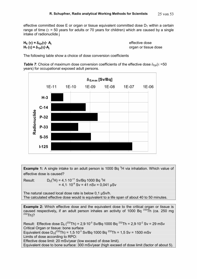
HE (ττττ) = δδδδEjk(ττττ)· Aj effective dose HT (ττττ) = δδδδTjk(ττττ)·Aj organ or tissue dose The following table show a choice of dose conversion coefficients Table 7: Choice of maximum dose conversion coefficients of the effective dose δEjk(τ =50 years) for occupational exposed adult persons.
Example 1: A single intake to an adult person is 1000 Bq 3H via inhalation. Which value of effective dose is caused?
Result: DE(3H) = 4,1⋅10-11 Sv/Bq⋅1000 Bq 3H = 4,1⋅ 10-8 Sv = 41 nSv = 0,041 µSv The natural caused local dose rate is below 0,1 µSv/h. The calculated effective dose would is equivalent to a life span of about 40 to 50 minutes.
Example 2: Which effective dose and the equivalent dose to the critical organ or tissue is caused respectively, if an adult person inhales an activity of 1000 Bq 232Th (ca. 250 mg 232Th)? Result: Effective dose DE (232Th) = 2,9⋅10-5 Sv/Bq⋅1000 Bq 232Th = 2,9⋅10-2 Sv = 29 mSv Critical Organ or tissue: bone surface Equivalent dose DO(232Th) = 1,5⋅10-3 Sv/Bq⋅1000 Bq 232Th = 1,5 Sv = 1500 mSv Limits of dose according to RPO: Effective dose limit: 20 mSv/year (low exceed of dose limit). Equivalent dose to bone surface: 300 mSv/year (high exceed of dose limit (factor of about 5).
1E-11 1E-10 1E-09 1E-08 1E-07 1E-06
H-3
C-14
P-32
P-33
S-35
I-125
Ra
dio
nu
clid
e
δδδδ E,max [Sv/Bq]
R. Schupfner, Radio analytical Working Methods for Scientists 26 von 53
2.12.2 Incorporation monitoring 2.12.2.1 Requirement During all practices of radioactive substances an intake of radionuclides is not avoidable. As a consequence in addition to external exposure internal exposure is caused. The principle duties of radiation protection aim in the limitations of doses to an unavoidable minimum. Permanent incorporation monitoring must be executed if the effective dose HE(τ =50 years) and the organ dose HT(τ =50 years) caused by the intake exceed certain values. The doses are calculated according to the equations above. First, the unnoticed intake of the activity AU is calculated: AU = N·a·Ã where Ã: mean activity which is handled daily. N: number of handling days per year. a: portion of activity which is incorporated unnoticed. a can adopt the following values: a = 0,00001 in the case of not volatile radionuclides being handled in a digestorium a = 0,0001 in the case of not volatile radionuclides being handled outside a digestorium a = 0,001 in the case of labelling radionuclides of iodine a > 0,01 in the case of very volatile radionuclides e.g. 3H and 14C Calculating the exposure:
HE(τ =50 years, AU) = δEjk⋅ AU effective dose HT(τ =50 years, AU)= δOjk⋅ AU organ or tissue dose The dose conversion coefficients are taken assuming a intake by inhalation of class M. If HE(τ =50 years, AU) < 0,5 mSv
or HT(τ =50 years, AU) < 0,1HOL HOL: dose limits of organ doses according to RPO. 2.12.2.2 Procedure To perform the incorporation monitoring the following procedures are valid either alone or in combination including the determination of the activity concentration of the air of the activity in the body of the activity of excretion 2.12.2.3 Example: Standard incorporation monitoring in the case of handling 33P In following table 8 the required data are shown. It is assumed that a single intake occurs at the half of incorporation interval via inhalation with class M of AMAD2 5µm. A favourable detection method is LSC applying the low-level-LSC of type Quantulus 1220. 2 AMAD: Activity Median of Aerosol Diameter in the inhaled air.
R. Schupfner, Radio analytical Working Methods for Scientists 27 von 53
Table 8: Data to calculate the committed effective dose after inhalation of 33P Radionuclide 33P Half life time t1/2 25,34 d Mode of decay β
−
Maximum β−energy 200 keV Effective dose conversion coefficient δE,inh 1,3·10-9 Sv/Bq Monitoring interval ∆t 30 d Amount of the daily excreted urine 1600 mL Amount of sample 10 mL First, the daily excretion rate AX must be determined. At a counting time of 400 minutes the detection limit of about 0,0026 Bq/mL or about 4,1 Bq/d is realised. Second, the activity intake Aintake(½∆t) related to the half monitoring interval msut be calculated according the equation: Aintake(½∆t) =
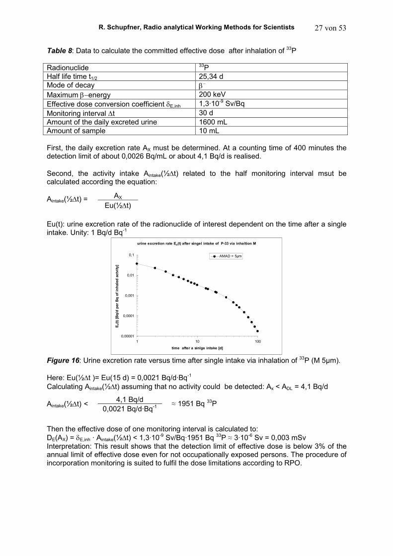
Eu(t): urine excretion rate of the radionuclide of interest dependent on the time after a single intake. Unity: 1 Bq/d Bq-1
urine excretion rate Eu(t) after singel intake of P-33 via inhaltion M
0,00001
0,0001
0,001
0,01
0,1
1 10 100
time after a sinlge intake [d]
Eu(t
) [B
q/d
per
Bq
of
inh
ale
d a
ctv
ity]
AMAD = 5µm
Figure 16: Urine excretion rate versus time after single intake via inhalation of 33P (M 5µm). Here: Eu(½∆t )= Eu(15 d) = 0,0021 Bq/d·Bq-1 Calculating Aintake(½∆t) assuming that no activity could be detected: Ax < ADL = 4,1 Bq/d Aintake(½∆t) < ≈ 1951 Bq 33P Then the effective dose of one monitoring interval is calculated to: DE(AX) = δE,inh · Aintake(½∆t) < 1,3·10-9 Sv/Bq·1951 Bq 33P ≈ 3·10-6 Sv = 0,003 mSv Interpretation: This result shows that the detection limit of effective dose is below 3% of the annual limit of effective dose even for not occupationally exposed persons. The procedure of incorporation monitoring is suited to fulfil the dose limitations according to RPO.
AX Eu(½∆t)
4,1 Bq/d 0,0021 Bq/d·Bq-1
R. Schupfner, Radio analytical Working Methods for Scientists 28 von 53
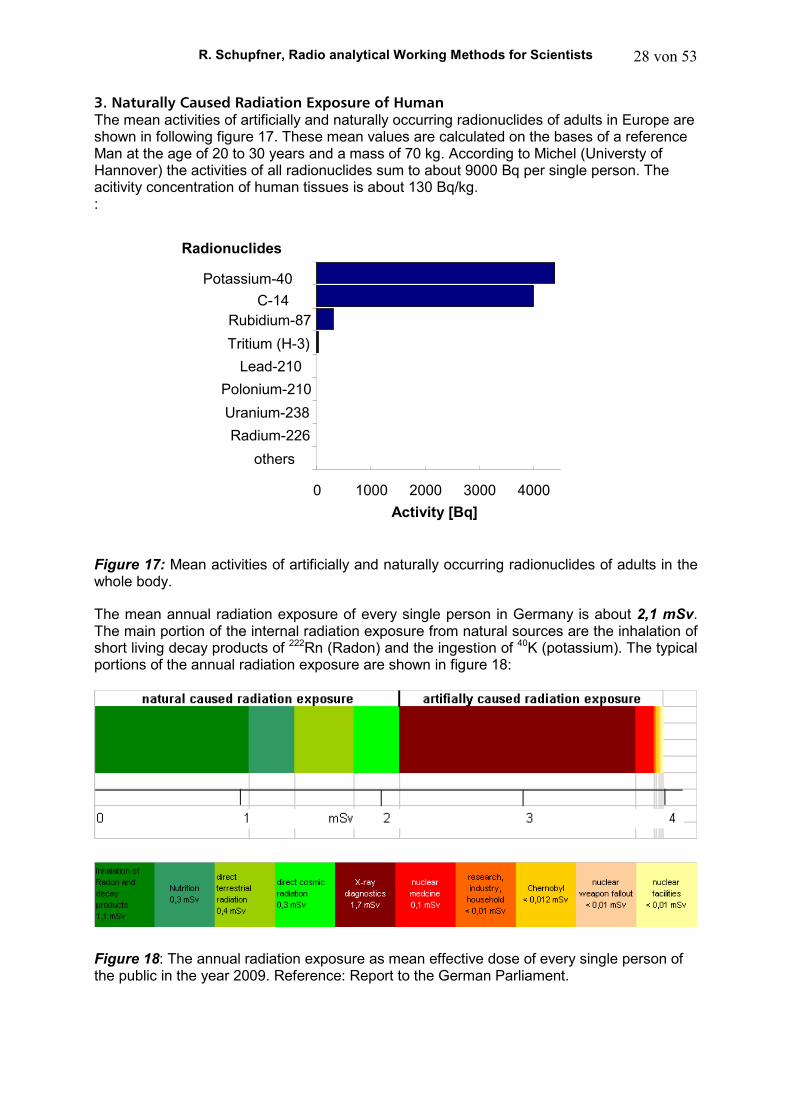
3. Naturally Caused Radiation Exposure of Human The mean activities of artificially and naturally occurring radionuclides of adults in Europe are shown in following figure 17. These mean values are calculated on the bases of a reference Man at the age of 20 to 30 years and a mass of 70 kg. According to Michel (Universty of Hannover) the activities of all radionuclides sum to about 9000 Bq per single person. The acitivity concentration of human tissues is about 130 Bq/kg. :
Figure 17: Mean activities of artificially and naturally occurring radionuclides of adults in the whole body.
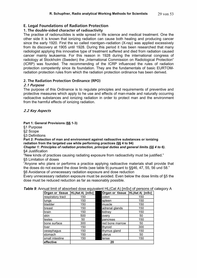
The mean annual radiation exposure of every single person in Germany is about 2,1 mSv. The main portion of the internal radiation exposure from natural sources are the inhalation of short living decay products of 222Rn (Radon) and the ingestion of 40K (potassium). The typical portions of the annual radiation exposure are shown in figure 18:
Figure 18: The annual radiation exposure as mean effective dose of every single person of the public in the year 2009. Reference: Report to the German Parliament.
0 1000 2000 3000 4000
Potassium-40
C-14Rubidium-87
Tritium (H-3)
Lead-210
Polonium-210
Uranium-238
Radium-226
others
Activity [Bq]
Radionuclides
R. Schupfner, Radio analytical Working Methods for Scientists 29 von 53
E. Legal Foundations of Radiation Protection 1. The double-sided character of radioactivity The practise of radionuclides is wide spread in life science and medical treatment. One the other side It is known that ionizing radiation can cause both healing and producing cancer since the early 1920. First the so called roentgen–radiation (X-ray) was applied excessively from its discovery at 1905 until 1928. During this period it has been researched that many radiologist applying this innovative type of treatment suffered and died from radiation caused cancer mainly leukaemia. For this reason in 1928 during the international congress of radiology at Stockholm (Sweden) the „International Commission on Radiological Protection“ (ICRP) was founded. The recommending of the ICRP influenced the rules of radiation protection competently since its foundation. They are the fundamentals of basic EURTOM- radiation protection rules from which the radiation protection ordinance has been derived. 2. The Radiation Protection Ordinance (RPO) 2.1 Purpose The purpose of this Ordinance is to regulate principles and requirements of preventive and protective measures which apply to he use and effects of man-made and naturally occurring radioactive substances and ionizing radiation in order to protect man and the environment from the harmful effects of ionizing radiation. 2.2 Key Aspects Part 1: General Provisions (§§ 1-3)
§1 Purpose §2 Scope §3 Definitions Part 2: Protection of man and environment against radioactive substances or ionizing radiation from the targeted use while performing practices (§§ 4 to 94)
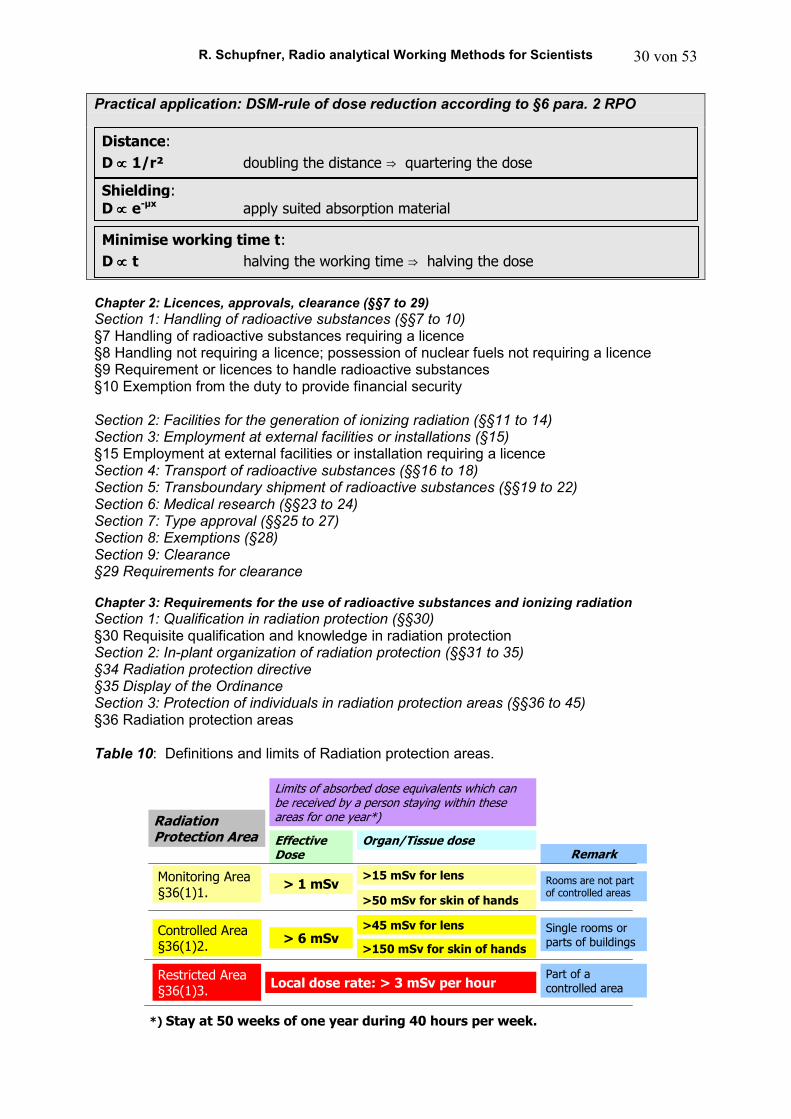
Chapter 1: Principles of radiation protection, principal duties and general limits (§§ 4 to 6). §4 Justification “New kinds of practices causing radiating exposure from radioactivity must be justified.” §5 Limitation of doses “Anyone who plans or performs a practice applying radioactive materials shall provide that the doses do not exceed the dose limits (see table 9) pursuant to §§46, 47, 55, 56 und 58.” §6 Avoidance of unnecessary radiation exposure and dose reduction Every unnecessary radiation exposure must be avoided. Even below the dose limits of §5 the dose must be reduced reduction as far as reasonably possible. Table 9: Annual limit of absorbed dose equivalent HL(Cat A) [mSv] of persons of category A
Organ or tissue HL(Aat A) [mSv] Organ or tissue HL(Aat A) [mSv]
respiratory tract 150 colon 150lungs 150 spleen 150bladder 150 muscle 150breast 150 adrenal glands 150brain 150 kidney 150skin 500 overy 50testes 50 pancreas 150bone surface 300 red bone marrow 50liver 150 thyroid 300oesephagus 150 thymus gland 150stomach 150 uterus 50small intestine 150 lense 150effective 20
R. Schupfner, Radio analytical Working Methods for Scientists 30 von 53
Practical application: DSM-rule of dose reduction according to §6 para. 2 RPO
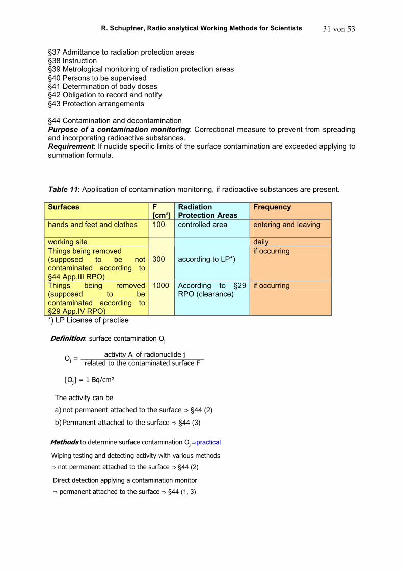
Chapter 2: Licences, approvals, clearance (§§7 to 29) Section 1: Handling of radioactive substances (§§7 to 10) §7 Handling of radioactive substances requiring a licence §8 Handling not requiring a licence; possession of nuclear fuels not requiring a licence §9 Requirement or licences to handle radioactive substances §10 Exemption from the duty to provide financial security Section 2: Facilities for the generation of ionizing radiation (§§11 to 14) Section 3: Employment at external facilities or installations (§15) §15 Employment at external facilities or installation requiring a licence Section 4: Transport of radioactive substances (§§16 to 18) Section 5: Transboundary shipment of radioactive substances (§§19 to 22) Section 6: Medical research (§§23 to 24) Section 7: Type approval (§§25 to 27) Section 8: Exemptions (§28) Section 9: Clearance §29 Requirements for clearance Chapter 3: Requirements for the use of radioactive substances and ionizing radiation Section 1: Qualification in radiation protection (§§30) §30 Requisite qualification and knowledge in radiation protection Section 2: In-plant organization of radiation protection (§§31 to 35) §34 Radiation protection directive §35 Display of the Ordinance Section 3: Protection of individuals in radiation protection areas (§§36 to 45) §36 Radiation protection areas Table 10: Definitions and limits of Radiation protection areas.
Monitoring Area §36(1)1.
Radiation Protection Area
Limits of absorbed dose equivalents which can be received by a person staying within these areas for one year*)
RemarkEffective Dose
Organ/Tissue dose
> 1 mSv>15 mSv for lens
>50 mSv for skin of hands
Rooms are not part of controlled areas
Controlled Area §36(1)2.
> 6 mSv>45 mSv for lens
>150 mSv for skin of hands
Single rooms or parts of buildings
Restricted Area §36(1)3.
Local dose rate: > 3 mSv per hourPart of a controlled area
*) Stay at 50 weeks of one year during 40 hours per week.
Distance:
D ∝∝∝∝ 1/r² doubling the distance ⇒ quartering the dose
Shielding:
D ∝∝∝∝ e-µx apply suited absorption material
Minimise working time t:
D ∝∝∝∝ t halving the working time ⇒ halving the dose
R. Schupfner, Radio analytical Working Methods for Scientists 31 von 53
§37 Admittance to radiation protection areas §38 Instruction §39 Metrological monitoring of radiation protection areas §40 Persons to be supervised §41 Determination of body doses §42 Obligation to record and notify §43 Protection arrangements §44 Contamination and decontamination Purpose of a contamination monitoring: Correctional measure to prevent from spreading and incorporating radioactive substances. Requirement: If nuclide specific limits of the surface contamination are exceeded applying to summation formula. Table 11: Application of contamination monitoring, if radioactive substances are present. Surfaces F
[cm²] Radiation Protection Areas
Frequency
hands and feet and clothes 100 controlled area entering and leaving
working site daily Things being removed (supposed to be not contaminated according to §44 App.III RPO)
300 according to LP*) if occurring
Things being removed (supposed to be contaminated according to §29 App.IV RPO)
1000 According to §29 RPO (clearance)
if occurring
*) LP License of practise Definition: surface contamination Oj
Oj =activity Aj of radionuclide j
related to the contaminated surface F
[Oj] = 1 Bq/cm²
The activity can be
a) not permanent attached to the surface ⇒ §44 (2)
b) Permanent attached to the surface ⇒ §44 (3) Methods to determine surface contamination Oj ⇒practical
Wiping testing and detecting activity with various methods
⇒ not permanent attached to the surface ⇒ §44 (2)
Direct detection applying a contamination monitor
⇒ permanent attached to the surface ⇒ §44 (1, 3)
R. Schupfner, Radio analytical Working Methods for Scientists 32 von 53
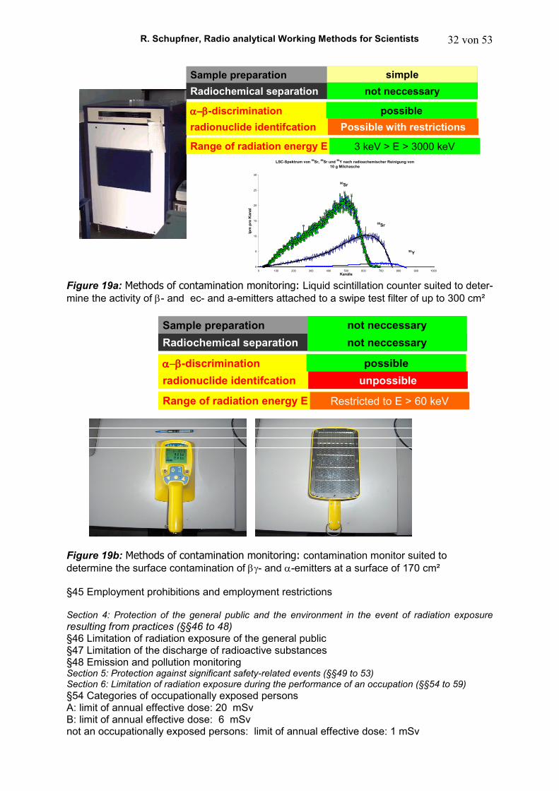
Radiochemical separation
Sample preparation simple
not neccessary
αααα−−−−ββββ-discrimination possible
radionuclide identifcation Possible with restrictions
Range of radiation energy E 3 keV > E > 3000 keVLSC-Spektrum von
90Sr,
89Sr und
90Y nach radioachemischer Reinigung von
10 g Milchasche
0
5
10
15
20
25
30
0 100 200 300 400 500 600 700 800 900 1000Kanäle
Ipm
pro
Kan
al
90Sr
90Y
89Sr
Figure 19a: Methods of contamination monitoring: Liquid scintillation counter suited to deter-mine the activity of β- and ec- and a-emitters attached to a swipe test filter of up to 300 cm²
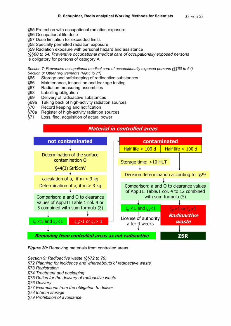
Radiochemical separation
Sample preparation not neccessary
not neccessary
αααα−−−−ββββ-discrimination possible
radionuclide identifcation unpossible
Range of radiation energy E Restricted to E > 60 keV
Figure 19b: Methods of contamination monitoring: contamination monitor suited to determine the surface contamination of βγ- and α-emitters at a surface of 170 cm² §45 Employment prohibitions and employment restrictions Section 4: Protection of the general public and the environment in the event of radiation exposure resulting from practices (§§46 to 48) §46 Limitation of radiation exposure of the general public §47 Limitation of the discharge of radioactive substances §48 Emission and pollution monitoring Section 5: Protection against significant safety-related events (§§49 to 53) Section 6: Limitation of radiation exposure during the performance of an occupation (§§54 to 59)
§54 Categories of occupationally exposed persons A: limit of annual effective dose: 20 mSv B: limit of annual effective dose: 6 mSv not an occupationally exposed persons: limit of annual effective dose: 1 mSv
R. Schupfner, Radio analytical Working Methods for Scientists 33 von 53
§55 Protection with occupational radiation exposure §56 Occupational life dose §57 Dose limitation for exceeded limits §58 Specially permitted radiation exposure §59 Radiation exposure with personal hazard and assistance (§§60 to 64: Preventive occupational medical care of occupationally exposed persons Is obligatory for persons of category A Section 7: Preventive occupational medical care of occupationally exposed persons (§§60 to 64) Section 8: Other requirements (§§65 to 71)
§65 Storage and safekeeping of radioactive substances §66 Maintenance, inspection and leakage testing §67 Radiation measuring assemblies §68 Labelling obligation §69 Delivery of radioactive substances §69a Taking back of high-activity radiation sources §70 Record keeping and notification §70a Register of high-activity radiation sources §71 Loss, find, acquisition of actual power
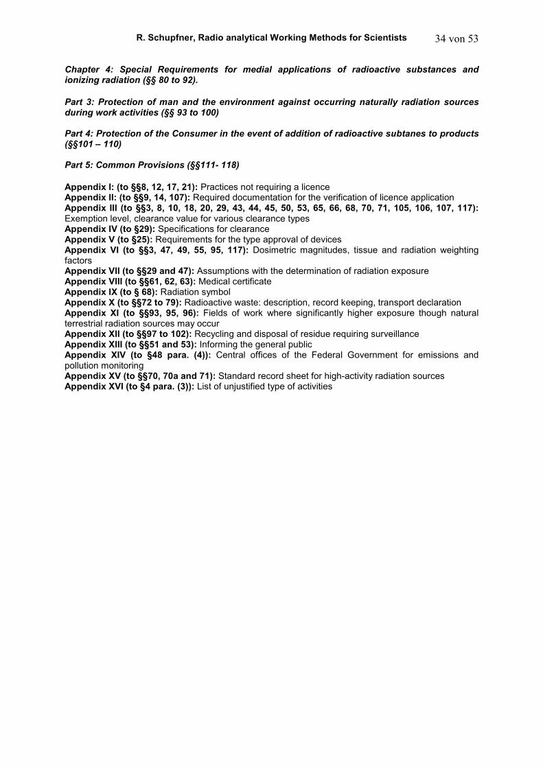
Material in controlled areas
Removing from controlled areas as not radioactive
not contaminated contaminated
Determination of the surface contamination O
§44(3) StrlSchV
calculation of a, if m < 3 kg
Determination of a, if m > 3 kg
Comparison: a and O to clearance values of App.III Table.1 col. 4 or 5 combined with sum formula (ξ)
ξΟ<1 and ξa<1 ξO>1 or ξa> 1
ZSR
Half life < 100 d Half life > 100 d
Storage time: >10·HLT
Decision determination according to §29
Comparison: a and O to clearance values of App.III Table.1 col. 4 to 12 combined
with sum formula (ξ)
ξΟ<1 and ξa<1
License of authority after 4 weeks
ξO>1 or ξa>1
Radioactive waste
Figure 20: Removing materials from controlled areas.
Section 9: Radioactive waste (§§72 to 79) §72 Planning for incidence and whereabouts of radioactive waste §73 Registration §74 Treatment and packaging §75 Duties for the delivery of radioactive waste §76 Delivery §77 Exemptions from the obligation to deliver §78 Interim storage §79 Prohibition of avoidance
R. Schupfner, Radio analytical Working Methods for Scientists 34 von 53
Chapter 4: Special Requirements for medial applications of radioactive substances and ionizing radiation (§§ 80 to 92). Part 3: Protection of man and the environment against occurring naturally radiation sources during work activities (§§ 93 to 100) Part 4: Protection of the Consumer in the event of addition of radioactive subtanes to products (§§101 – 110) Part 5: Common Provisions (§§111- 118) Appendix I: (to §§8, 12, 17, 21): Practices not requiring a licence Appendix II: (to §§9, 14, 107): Required documentation for the verification of licence application Appendix III (to §§3, 8, 10, 18, 20, 29, 43, 44, 45, 50, 53, 65, 66, 68, 70, 71, 105, 106, 107, 117):
Exemption level, clearance value for various clearance types Appendix IV (to §29): Specifications for clearance Appendix V (to §25): Requirements for the type approval of devices Appendix VI (to §§3, 47, 49, 55, 95, 117): Dosimetric magnitudes, tissue and radiation weighting factors Appendix VII (to §§29 and 47): Assumptions with the determination of radiation exposure Appendix VIII (to §§61, 62, 63): Medical certificate Appendix IX (to § 68): Radiation symbol Appendix X (to §§72 to 79): Radioactive waste: description, record keeping, transport declaration Appendix XI (to §§93, 95, 96): Fields of work where significantly higher exposure though natural terrestrial radiation sources may occur Appendix XII (to §§97 to 102): Recycling and disposal of residue requiring surveillance Appendix XIII (to §§51 and 53): Informing the general public Appendix XIV (to §48 para. (4)): Central offices of the Federal Government for emissions and pollution monitoring Appendix XV (to §§70, 70a and 71): Standard record sheet for high-activity radiation sources Appendix XVI (to §4 para. (3)): List of unjustified type of activities
R. Schupfner, Radio analytical Working Methods for Scientists 35 von 53
F. Methods of Detection of Nuclear Radiation 1. Single Nuclide Determination
The basic equation to determine the activity detecting the nuclear radiation of one single radionuclide is: R = yi·ηphys·ηchem·A where: R = R´ - R0 is the net counting rate at the beginning of the counting time and R´= gross counting rate ΣI´: Sum of counts caused by both together radioactivity of the sample and blank background counting rate during the life time tL of the sample detection. R0 = R0 (t0) = background counting rate I0: Number of background counts during the counting time t0 Unit: [R] = 1 count per second = 1 cps or 1 count per minute =1 cpm
ηphys: absolute counting efficiency ηchem: chemical yield in % yi: Emission probability of an observed radiation i caused by a nuclear transition Unity: [yi] = 1 (Bqs)-1 = 100% A(0): Activity at the beginning of counting time If tM << t1/2: The decay of the radionuclide during the counting time can be neglected. The activity does not change significantly: A(0) ≈ A(tM). Then it is true: R´(0) = R´(tM) = gross counting rate with I´: Sum of counts of sample and background. If: tM ≥ t1/2: The decay of the radionuclide during the counting time can be not neglected. The activity change significantly. It is: R(0) = I0(tM): Number of counts caused by background counting 2. Multi Nuclide Determination The net counting rate R caused by radioactive samples containing more than one radionuclide the sum of the counting rates of every singe radionuclide is: R = R1 + R2 + … = η·A1 + η2·A2 + … If all yi = 1 and ηchem.= 1.
ΣI´ tL
I0 t0
I´(tM) tM
λ·[I´(tM)-I0(tM)] 1-e−λ·tM
R. Schupfner, Radio analytical Working Methods for Scientists 36 von 53
3. Determination of Activity 3.1 Basic Radioanalytical Equation The activity can be determined by following equation: A = R/(yi·ηphys·ηchem) 3.2 Counting Efficiency ηPhy
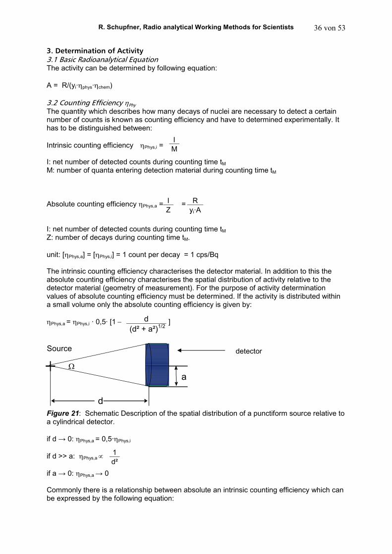
The quantity which describes how many decays of nuclei are necessary to detect a certain number of counts is known as counting efficiency and have to determined experimentally. It has to be distinguished between: Intrinsic counting efficiency ηPhys,i = I: net number of detected counts during counting time tM M: number of quanta entering detection material during counting time tM Absolute counting efficiency ηPhys,a = = I: net number of detected counts during counting time tM Z: number of decays during counting time tM. unit: [ηPhys,a] = [ηPhys,i] = 1 count per decay = 1 cps/Bq The intrinsic counting efficiency characterises the detector material. In addition to this the absolute counting efficiency characterises the spatial distribution of activity relative to the detector material (geometry of measurement). For the purpose of activity determination values of absolute counting efficiency must be determined. If the activity is distributed within a small volume only the absolute counting efficiency is given by: ηPhys,a = ηPhys,i · 0,5· [1 − ]
Figure 21: Schematic Description of the spatial distribution of a punctiform source relative to a cylindrical detector. if d → 0: ηPhys,a = 0,5·ηPhys,i if d >> a: ηPhys,a ∝
if a → 0: ηPhys,a → 0 Commonly there is a relationship between absolute an intrinsic counting efficiency which can be expressed by the following equation:
I M
I Z
d (d² + a²)1/2
R yi ·A
1 d²
Source
a
d
Ω
detector
R. Schupfner, Radio analytical Working Methods for Scientists 37 von 53
ηηηηPhys, a (E) = (1-S)·(1+B)·G·(1-W)·ηηηηPhys, i (E) The absolute counting efficiency ηPhys,a depends on the following factors:
• Detector material influencing the value of the intrinsic counting efficiency ηPhys, i • Detector geometry G (volume and shape) • Surrounding shielding material of detector influencing the value of the backscatter B • Sample material (Self absorption of sample material S) • Distance between source of activity and detector influencing the value of self
absorption in air W • Distribution of the activity relative to the detector G • Type of the emitted ionizing radiation (α, β, γ) • Energy E of the emitted ionizing radiation
3.3 Calibration Factor κ
The calibration factor κ can be calculated from the absolute counting efficiency ηPhys,a and emission probability yi according to the equation. κ = Unit: [κA] = 1 decay/count = 1 Bq/cps, if the magnitude of interest is activity Unit: [κO] = 1 Bq/(cps·cm²), if the magnitude of interest is surface contamination O The purpose defining the magnitude of calibration factor is to simply the calculation of activity. Determining the activity A according the equation: A = κκκκA ·R net counting rate R or determining the surface contamination O according the equation: O = κκκκO ·R net counting rate R Frequently applied to contamination monitors. 3.4 Dead Time tD
During a certain range of time called dead time tD the detection device is not able to register counts. The dead time is determined relative to the real counting time tR (real time) tD [%] = 100· The dead time is dependent on activity A and absolute counting efficiency ηPhys,a. 3.5 Counting Uncertainty Radioactive decay fits the Poisson distribution (see figure 7 above). Therefore it is not possible to predict the precise time at which a single decay occurs. As a consequence the counting rate is always combined to a statistical uncertainty. If the number of pulses I of a long-living radionuclide is detected again and again (n times) under identical conditions a distribution of the gross counts Ii´ is observed deviating round the mean value δ δ= = Σ Ii´ The width of variance is characterized by the standard deviation σ which is calculated as square root of the variance σ²: σ² =
1 yi·ηPhys,a
tR-tL tR
I1´ + I2´ + I3´ + … + In´ n
1 n
Σ(Ii´ - δ)² n
R. Schupfner, Radio analytical Working Methods for Scientists 38 von 53
If n → ∞ and small values δ< 20 the Poisson distribution is valid (see figure 7 above): At higher values of I´ the asymmetric Poisson distribution fits the symmetric Gaussian distribution. According to this distribution there are different probabilities that the number of pulses are within the following intervals Ii´- Î< 1 σ for a probability of 68,3 % and Ii´- Î< 1,96σ for a probability of 95% and Ii´- Î< 3σ for a probability of 99,7%. If the Poisson distribution is valid it is true: σ = ± √δ Example: I´= 10.000 counts (abbreviated as cts) ______ The counting uncertainty ∆I´ is calculated according: ∆I´ ≈ σ = √10.000 cts = 100 cts. Relative counting uncertainty is calculated according: ∆I´/I´ = 100 cts/10.000 cts = 1%. Because of the Poisson distribution of the frequencies of the numbers of decay and the linear relation between the number of decays n and the detected gross counts I´ the standard deviation of I´ named ∆I´ can be easily calculated according to the equation: _
∆I´ ≈ σ = √I´ The standard deviation ∆I0´ of the background counts is: _
∆I0 ≈ σ0 = √I0 If it is assumed that the standard deviation approximately equal to the counting uncertainty the uncertainty ∆R of the net counting rate R can be calculated. R = R´- R0 = I`/tM – I0/t0 __________ ∆R = √ ∆R´² + ∆R0² where _ _
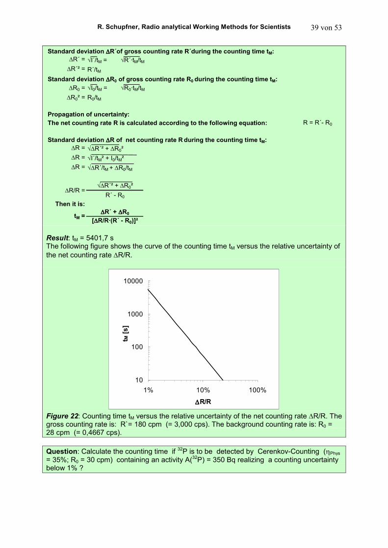
∆R´ = ∆I`/tM = √I´/tM and ∆R0 = ∆I`/t0 = √I0/t0 ∆R´² = I´/tM² and ∆R0² = I0/t0² __________ Then it is: ∆R = √I´/tM² + I0/t0² If the counting times of sample and background are equal tM = t0 = t the equation above simplifies to _____ ∆R = √I´ + I0/t Example: Calculate the counting time tM under the following conditions to detect 32P applying Cerencov counting with a LSC of type “TRIATHLER” to assure a difference of the net counting rate of more than 2%. The gross counting rate is: R`= 180 cpm (= 3,000 cps) The background counting rate is: R0 = 28 cpm (= 0,4667 cps) Applying the Poisson distribution of the gross counts:
R. Schupfner, Radio analytical Working Methods for Scientists 39 von 53
Standard deviation ∆∆∆∆R´of gross counting rate R´during the counting time tM:
∆R´ = √I´/tM = √R´·tM/tM∆R´² = R´/tM
Standard deviation ∆∆∆∆R0 of gross counting rate R0 during the counting time tM:
∆R0 = √I0/tM = √R0·tM/tM
∆R0² = R0/tM
Propagation of uncertainty:
The net counting rate R is calculated according to the following equation: R = R´- R0
Standard deviation ∆∆∆∆R of net counting rate R during the counting time tM:
∆R = √∆R´² + ∆R0²∆R = √I´/tM² + I0/tM²∆R = √∆R´/tM + ∆R0/tM
Then it is:
tM =∆∆∆∆R´ + ∆∆∆∆R0
[∆∆∆∆R/R·(R´ - R0)]²
∆R/R =R´ - R0
√∆R´² + ∆R0²
Result: tM = 5401,7 s The following figure shows the curve of the counting time tM versus the relative uncertainty of the net counting rate ∆R/R.
10
100
1000
10000
1% 10% 100%
∆∆∆∆R/R
t M [
s]
Figure 22: Counting time tM versus the relative uncertainty of the net counting rate ∆R/R. The gross counting rate is: R`= 180 cpm (= 3,000 cps). The background counting rate is: R0 = 28 cpm (= 0,4667 cps). Question: Calculate the counting time if 32P is to be detected by Cerenkov-Counting (ηPhys = 35%; R0 = 30 cpm) containing an activity A(32P) = 350 Bq realizing a counting uncertainty below 1% ?
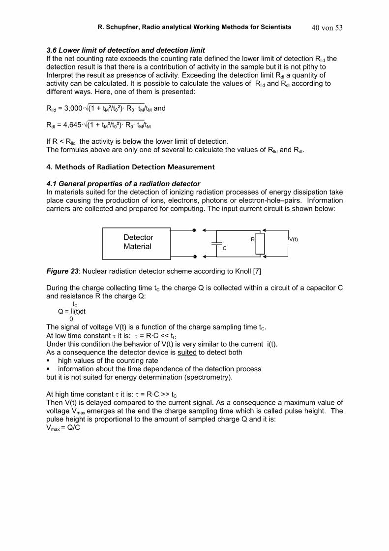
R. Schupfner, Radio analytical Working Methods for Scientists 40 von 53
3.6 Lower limit of detection and detection limit If the net counting rate exceeds the counting rate defined the lower limit of detection Rlld the detection result is that there is a contribution of activity in the sample but it is not pithy to Interpret the result as presence of activity. Exceeding the detection limit Rdl a quantity of activity can be calculated. It is possible to calculate the values of Rlld and Rdl according to different ways. Here, one of them is presented: ______________ Rlld = 3,000·√(1 + tM²/t0²)· R0· tM/tM and ______________ Rdl = 4,645·√(1 + tM²/t0²)· R0· tM/tM If R < Rlld the activity is below the lower limit of detection. The formulas above are only one of several to calculate the values of Rlld and Rdl. 4. Methods of Radiation Detection Measurement 4.1 General properties of a radiation detector In materials suited for the detection of ionizing radiation processes of energy dissipation take place causing the production of ions, electrons, photons or electron-hole–pairs. Information carriers are collected and prepared for computing. The input current circuit is shown below:
Figure 23: Nuclear radiation detector scheme according to Knoll [7] During the charge collecting time tC the charge Q is collected within a circuit of a capacitor C and resistance R the charge Q:
tC Q = ∫i(t)dt
0 The signal of voltage V(t) is a function of the charge sampling time tC. At low time constant τ it is: τ = R·C << tC Under this condition the behavior of V(t) is very similar to the current i(t). As a consequence the detector device is suited to detect both high values of the counting rate information about the time dependence of the detection process but it is not suited for energy determination (spectrometry). At high time constant τ it is: τ = R·C >> tC Then V(t) is delayed compared to the current signal. As a consequence a maximum value of voltage Vmax emerges at the end the charge sampling time which is called pulse height. The pulse height is proportional to the amount of sampled charge Q and it is: Vmax = Q/C
R V(t)
C Detector Material
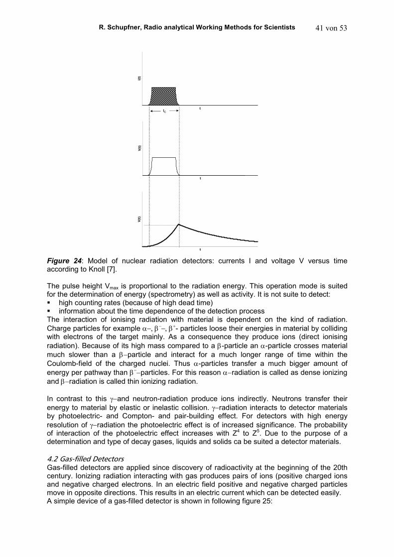
R. Schupfner, Radio analytical Working Methods for Scientists 41 von 53
t
i(t)
tC
t
V(t
)
t
V(t
)
Figure 24: Model of nuclear radiation detectors: currents I and voltage V versus time according to Knoll [7]. The pulse height Vmax is proportional to the radiation energy. This operation mode is suited for the determination of energy (spectrometry) as well as activity. It is not suite to detect: high counting rates (because of high dead time) information about the time dependence of the detection process The interaction of ionising radiation with material is dependent on the kind of radiation. Charge particles for example α−, β
−−, β
+- particles loose their energies in material by colliding with electrons of the target mainly. As a consequence they produce ions (direct ionising radiation). Because of its high mass compared to a β-particle an α-particle crosses material much slower than a β−particle and interact for a much longer range of time within the Coulomb-field of the charged nuclei. Thus α-particles transfer a much bigger amount of energy per pathway than β−
−particles. For this reason α−radiation is called as dense ionizing and β−radiation is called thin ionizing radiation. In contrast to this γ−and neutron-radiation produce ions indirectly. Neutrons transfer their energy to material by elastic or inelastic collision. γ−radiation interacts to detector materials by photoelectric- and Compton- and pair-building effect. For detectors with high energy resolution of γ−radiation the photoelectric effect is of increased significance. The probability of interaction of the photoelectric effect increases with Z4 to Z5. Due to the purpose of a determination and type of decay gases, liquids and solids ca be suited a detector materials. 4.2 Gas-filled Detectors Gas-filled detectors are applied since discovery of radioactivity at the beginning of the 20th century. Ionizing radiation interacting with gas produces pairs of ions (positive charged ions and negative charged electrons. In an electric field positive and negative charged particles move in opposite directions. This results in an electric current which can be detected easily. A simple device of a gas-filled detector is shown in following figure 25:
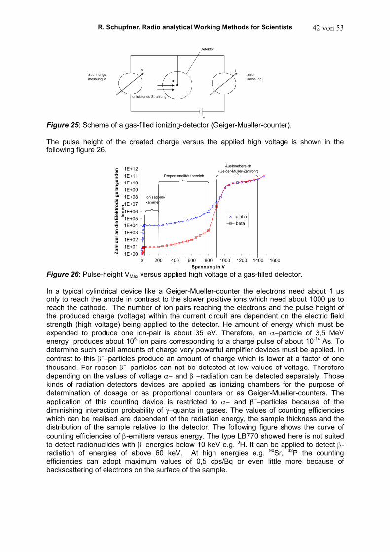
R. Schupfner, Radio analytical Working Methods for Scientists 42 von 53
Figure 25: Scheme of a gas-filled ionizing-detector (Geiger-Mueller-counter). The pulse height of the created charge versus the applied high voltage is shown in the following figure 26. Figure 26: Pulse-height VMax versus applied high voltage of a gas-filled detector. In a typical cylindrical device like a Geiger-Mueller-counter the electrons need about 1 µs only to reach the anode in contrast to the slower positive ions which need about 1000 µs to reach the cathode. The number of ion pairs reaching the electrons and the pulse height of the produced charge (voltage) within the current circuit are dependent on the electric field strength (high voltage) being applied to the detector. He amount of energy which must be expended to produce one ion-pair is about 35 eV. Therefore, an α−particle of 3,5 MeV energy produces about 105 ion pairs corresponding to a charge pulse of about 10-14 As. To determine such small amounts of charge very powerful amplifier devices must be applied. In contrast to this β−
−particles produce an amount of charge which is lower at a factor of one thousand. For reason β
−−particles can not be detected at low values of voltage. Therefore
depending on the values of voltage α− and β−−radiation can be detected separately. Those
kinds of radiation detectors devices are applied as ionizing chambers for the purpose of determination of dosage or as proportional counters or as Geiger-Mueller-counters. The application of this counting device is restricted to α− and β
−−particles because of the
diminishing interaction probability of γ−quanta in gases. The values of counting efficiencies which can be realised are dependent of the radiation energy, the sample thickness and the distribution of the sample relative to the detector. The following figure shows the curve of counting efficiencies of β-emitters versus energy. The type LB770 showed here is not suited to detect radionuclides with β−energies below 10 keV e.g. 3H. It can be applied to detect β-radiation of energies of above 60 keV. At high energies e.g. 90Sr, 32P the counting efficiencies can adopt maximum values of 0,5 cps/Bq or even little more because of backscattering of electrons on the surface of the sample.
Detektor
V iSpannungs- Strom-messung V messung i
ionisierende Strahlung
- +
1E+001E+011E+021E+031E+041E+051E+06
1E+071E+081E+091E+101E+111E+12
0 200 400 600 800 1000 1200 1400 1600Spannung in V
Za
hl d
er
an
die
Ele
ktr
od
e g
ela
ng
en
den
Ion
en
alphabeta
Ionisations-kammer
Proportionalitätsbereich
Auslösebereich (Geiger-Müller-Zählrohr)
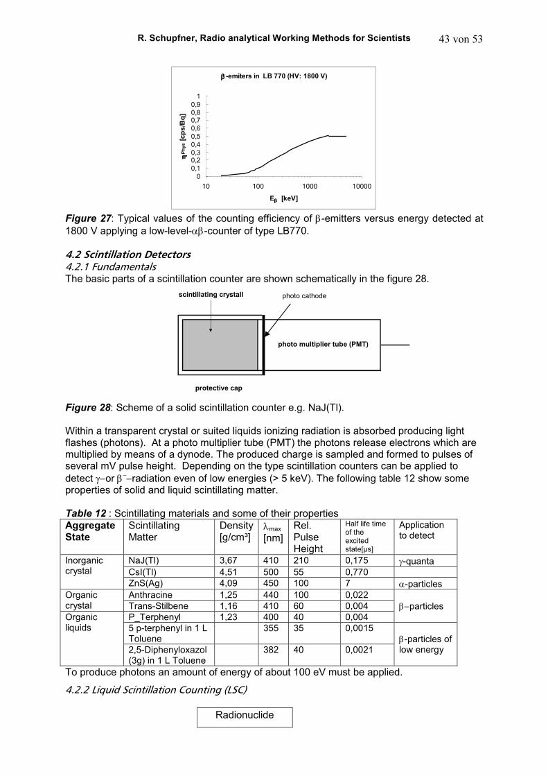
R. Schupfner, Radio analytical Working Methods for Scientists 43 von 53
ββββ -emiters in LB 770 (HV: 1800 V)
00,10,20,30,40,50,60,70,80,9
1
10 100 1000 10000
Eββββ [keV]
ηη ηηP
hys [
cp
s/B
q]
Figure 27: Typical values of the counting efficiency of β-emitters versus energy detected at 1800 V applying a low-level-αβ-counter of type LB770. 4.2 Scintillation Detectors 4.2.1 Fundamentals The basic parts of a scintillation counter are shown schematically in the figure 28.
Kristall Photkathode
Schutzkappe
Photomultiplier
scintillating crystall
protective cap
photo cathode
photo multiplier tube (PMT)
Figure 28: Scheme of a solid scintillation counter e.g. NaJ(Tl). Within a transparent crystal or suited liquids ionizing radiation is absorbed producing light flashes (photons). At a photo multiplier tube (PMT) the photons release electrons which are multiplied by means of a dynode. The produced charge is sampled and formed to pulses of several mV pulse height. Depending on the type scintillation counters can be applied to detect γ−or β−
−radiation even of low energies (> 5 keV). The following table 12 show some properties of solid and liquid scintillating matter. Table 12 : Scintillating materials and some of their properties Aggregate State
Scintillating Matter
Density [g/cm³]
λmax [nm]
Rel. Pulse Height
Half life time of the excited state[µs]
Application to detect
NaJ(Tl) 3,67 410 210 0,175 γ-quanta CsI(Tl) 4,51 500 55 0,770
Inorganic crystal
ZnS(Ag) 4,09 450 100 7 α-particles Anthracine 1,25 440 100 0,022 Organic
crystal Trans-Stilbene 1,16 410 60 0,004 P_Terphenyl 1,23 400 40 0,004
β−particles
5 p-terphenyl in 1 L Toluene
355 35 0,0015 Organic liquids
2,5-Diphenyloxazol (3g) in 1 L Toluene
382 40 0,0021 β-particles of low energy
To produce photons an amount of energy of about 100 eV must be applied.
4.2.2 Liquid Scintillation Counting (LSC)
Radionuclide
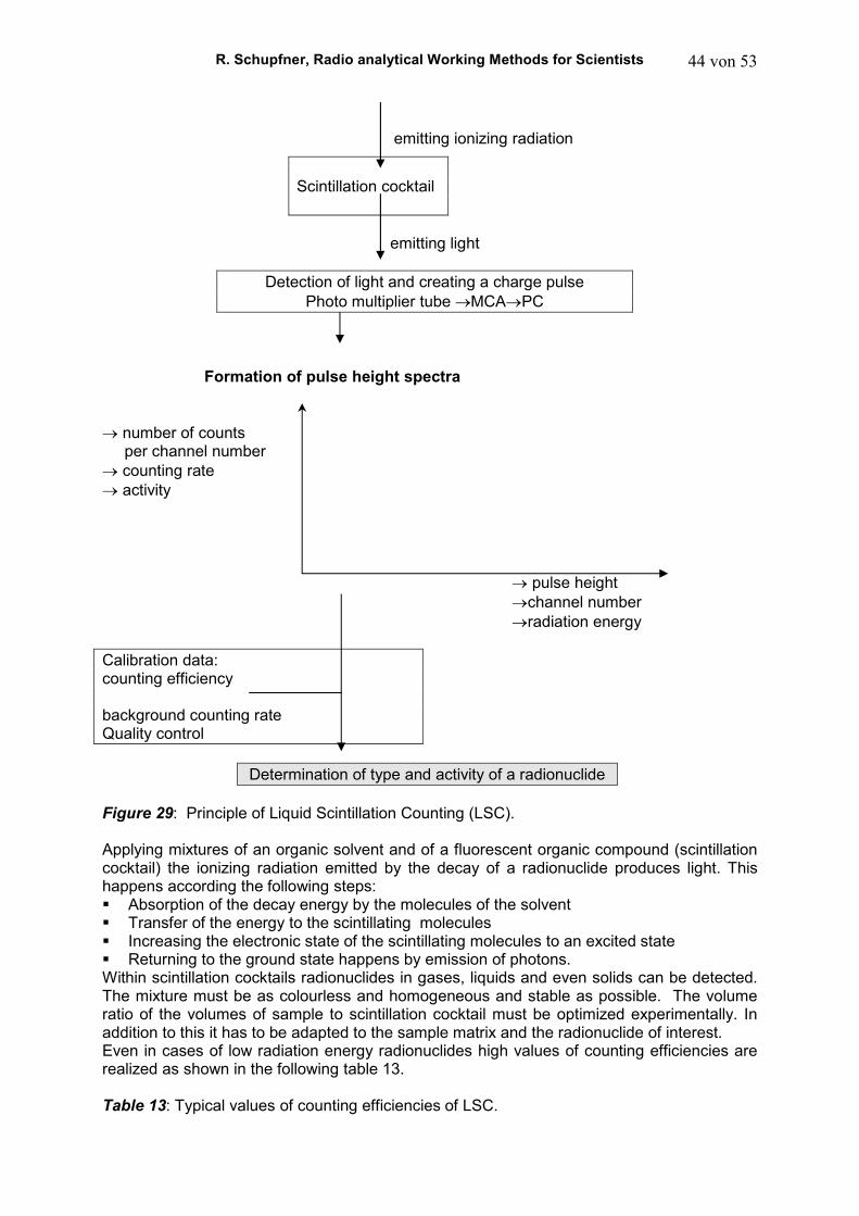
R. Schupfner, Radio analytical Working Methods for Scientists 44 von 53
emitting ionizing radiation
Scintillation cocktail
emitting light
Detection of light and creating a charge pulse
Photo multiplier tube →MCA→PC
Formation of pulse height spectra
→ number of counts per channel number → counting rate → activity
→ pulse height →channel number →radiation energy Calibration data: counting efficiency background counting rate Quality control
Determination of type and activity of a radionuclide Figure 29: Principle of Liquid Scintillation Counting (LSC). Applying mixtures of an organic solvent and of a fluorescent organic compound (scintillation cocktail) the ionizing radiation emitted by the decay of a radionuclide produces light. This happens according the following steps: Absorption of the decay energy by the molecules of the solvent Transfer of the energy to the scintillating molecules Increasing the electronic state of the scintillating molecules to an excited state Returning to the ground state happens by emission of photons. Within scintillation cocktails radionuclides in gases, liquids and even solids can be detected. The mixture must be as colourless and homogeneous and stable as possible. The volume ratio of the volumes of sample to scintillation cocktail must be optimized experimentally. In addition to this it has to be adapted to the sample matrix and the radionuclide of interest. Even in cases of low radiation energy radionuclides high values of counting efficiencies are realized as shown in the following table 13. Table 13: Typical values of counting efficiencies of LSC.
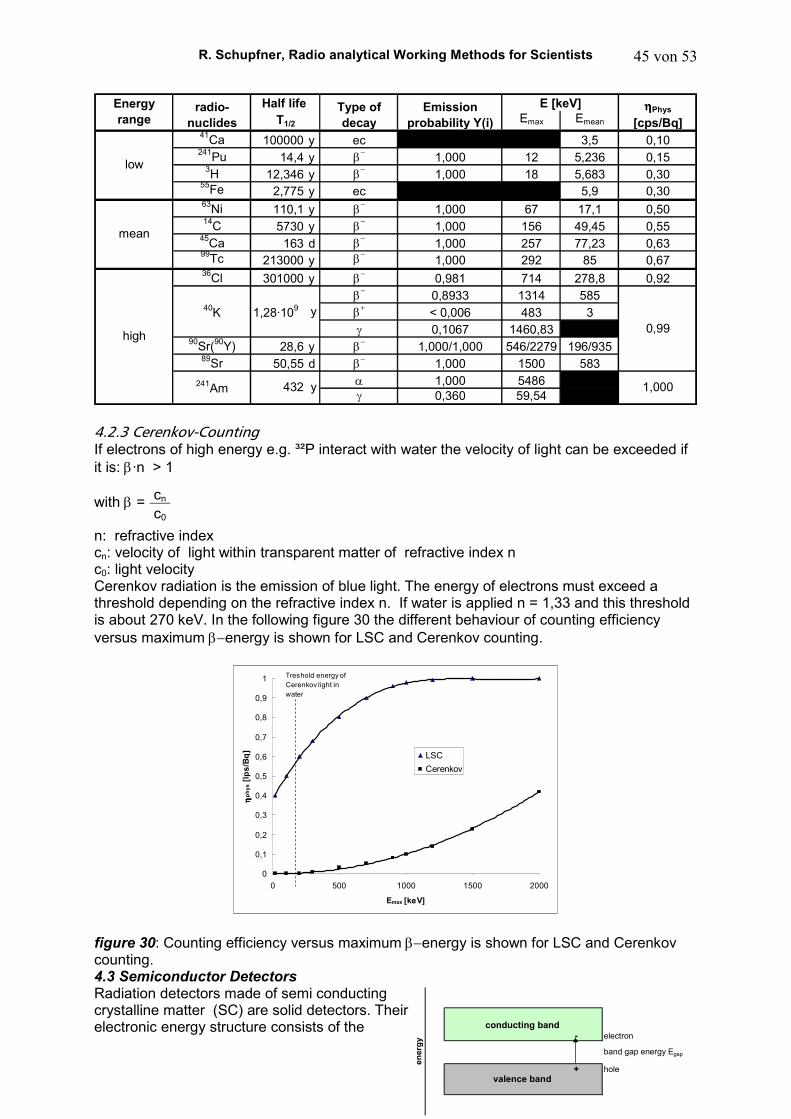
R. Schupfner, Radio analytical Working Methods for Scientists 45 von 53
Emax Emean
41Ca 100000 y ec 3,5 0,10241Pu 14,4 y β
− 1,000 12 5,236 0,153H 12,346 y β
− 1,000 18 5,683 0,3055Fe 2,775 y ec 5,9 0,3063Ni 110,1 y β
− 1,000 67 17,1 0,5014C 5730 y β
− 1,000 156 49,45 0,5545Ca 163 d β
− 1,000 257 77,23 0,6399Tc 213000 y β
−1,000 292 85 0,67
36Cl 301000 y β− 0,981 714 278,8 0,92
β− 0,8933 1314 585
β+ < 0,006 483 3
γ 0,1067 1460,8390Sr(90Y) 28,6 y β
− 1,000/1,000 546/2279 196/93589Sr 50,55 d β
− 1,000 1500 583α 1,000 5486γ 0,360 59,54
ηηηηPhys
[cps/Bq]
0,99
1,000
y
241Am 432 y
mean
high
40K 1,28·109
E [keV]
T1/2
Half life
low
radio-
nuclides
Energy
rangeType of
decay
Emission
probability Y(i)
4.2.3 Cerenkov-Counting If electrons of high energy e.g. ³²P interact with water the velocity of light can be exceeded if it is: β·n > 1 with β = n: refractive index cn: velocity of light within transparent matter of refractive index n c0: light velocity Cerenkov radiation is the emission of blue light. The energy of electrons must exceed a threshold depending on the refractive index n. If water is applied n = 1,33 and this threshold is about 270 keV. In the following figure 30 the different behaviour of counting efficiency versus maximum β−energy is shown for LSC and Cerenkov counting.
0
0,1
0,2
0,3
0,4
0,5
0,6
0,7
0,8
0,9
1
0 500 1000 1500 2000
Emax [keV]
ηη ηηp
hy
s [
Ips
/Bq
] LSC
Cerenkov
Treshold energy of Cerenkov light in water
figure 30: Counting efficiency versus maximum β−energy is shown for LSC and Cerenkov counting. 4.3 Semiconductor Detectors Radiation detectors made of semi conducting crystalline matter (SC) are solid detectors. Their electronic energy structure consists of the
cn c0
- electron
+ hole
band gap energy Egap
en
erg
y
valence band
conducting band
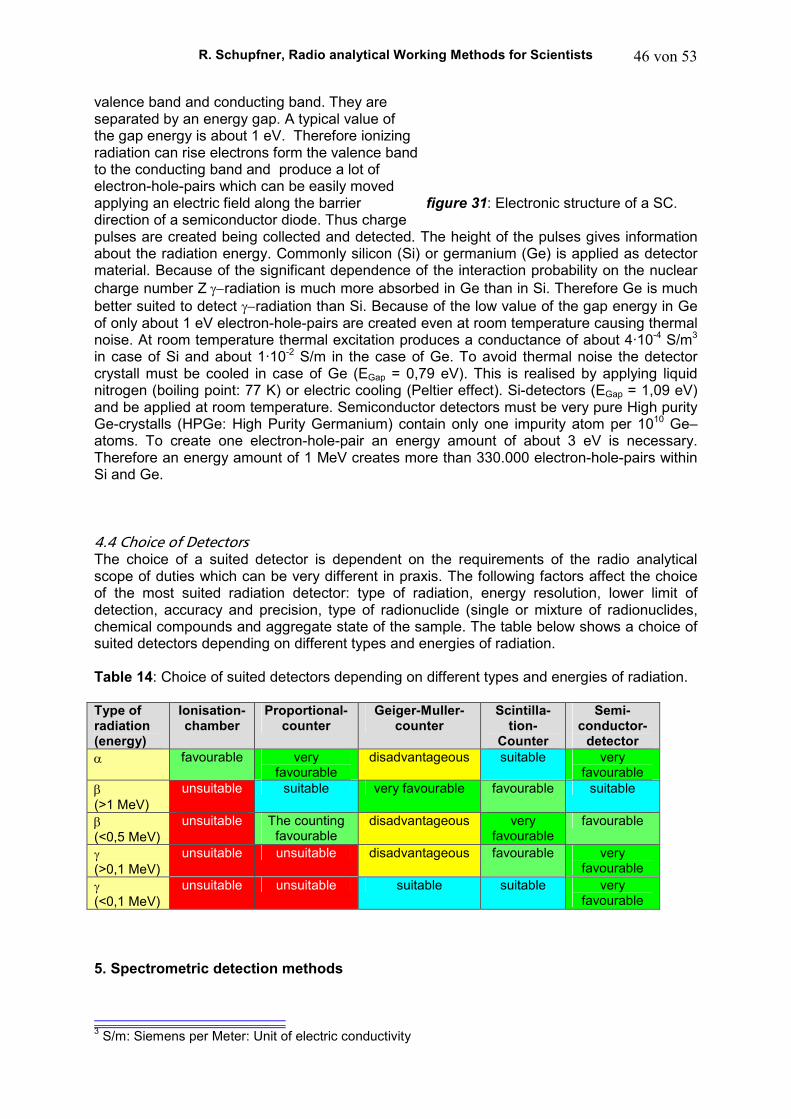
R. Schupfner, Radio analytical Working Methods for Scientists 46 von 53
valence band and conducting band. They are separated by an energy gap. A typical value of the gap energy is about 1 eV. Therefore ionizing radiation can rise electrons form the valence band to the conducting band and produce a lot of electron-hole-pairs which can be easily moved applying an electric field along the barrier figure 31: Electronic structure of a SC. direction of a semiconductor diode. Thus charge pulses are created being collected and detected. The height of the pulses gives information about the radiation energy. Commonly silicon (Si) or germanium (Ge) is applied as detector material. Because of the significant dependence of the interaction probability on the nuclear charge number Z γ−radiation is much more absorbed in Ge than in Si. Therefore Ge is much better suited to detect γ−radiation than Si. Because of the low value of the gap energy in Ge of only about 1 eV electron-hole-pairs are created even at room temperature causing thermal noise. At room temperature thermal excitation produces a conductance of about 4·10-4 S/m3 in case of Si and about 1·10-2 S/m in the case of Ge. To avoid thermal noise the detector crystall must be cooled in case of Ge (EGap = 0,79 eV). This is realised by applying liquid nitrogen (boiling point: 77 K) or electric cooling (Peltier effect). Si-detectors (EGap = 1,09 eV) and be applied at room temperature. Semiconductor detectors must be very pure High purity Ge-crystalls (HPGe: High Purity Germanium) contain only one impurity atom per 1010 Ge–atoms. To create one electron-hole-pair an energy amount of about 3 eV is necessary. Therefore an energy amount of 1 MeV creates more than 330.000 electron-hole-pairs within Si and Ge. 4.4 Choice of Detectors The choice of a suited detector is dependent on the requirements of the radio analytical scope of duties which can be very different in praxis. The following factors affect the choice of the most suited radiation detector: type of radiation, energy resolution, lower limit of detection, accuracy and precision, type of radionuclide (single or mixture of radionuclides, chemical compounds and aggregate state of the sample. The table below shows a choice of suited detectors depending on different types and energies of radiation. Table 14: Choice of suited detectors depending on different types and energies of radiation. Type of radiation (energy)
Ionisation-chamber
Proportional-counter
Geiger-Muller- counter
Scintilla-tion-
Counter
Semi- conductor-
detector
α favourable very favourable
disadvantageous suitable very favourable
β
(>1 MeV) unsuitable suitable very favourable favourable suitable
β (<0,5 MeV)
unsuitable The counting favourable
disadvantageous very favourable
favourable
γ (>0,1 MeV)
unsuitable unsuitable disadvantageous favourable very favourable
γ (<0,1 MeV)
unsuitable unsuitable suitable suitable very favourable
5. Spectrometric detection methods
3 S/m: Siemens per Meter: Unit of electric conductivity
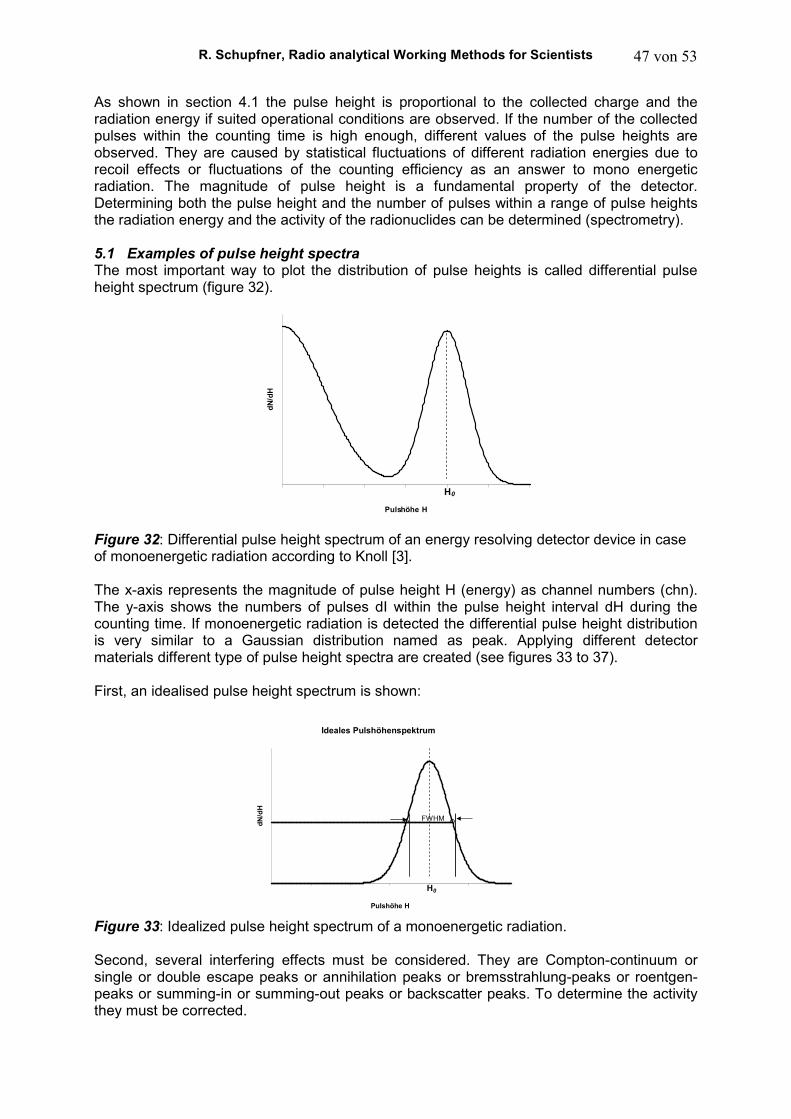
R. Schupfner, Radio analytical Working Methods for Scientists 47 von 53
As shown in section 4.1 the pulse height is proportional to the collected charge and the radiation energy if suited operational conditions are observed. If the number of the collected pulses within the counting time is high enough, different values of the pulse heights are observed. They are caused by statistical fluctuations of different radiation energies due to recoil effects or fluctuations of the counting efficiency as an answer to mono energetic radiation. The magnitude of pulse height is a fundamental property of the detector. Determining both the pulse height and the number of pulses within a range of pulse heights the radiation energy and the activity of the radionuclides can be determined (spectrometry). 5.1 Examples of pulse height spectra The most important way to plot the distribution of pulse heights is called differential pulse height spectrum (figure 32). Figure 32: Differential pulse height spectrum of an energy resolving detector device in case of monoenergetic radiation according to Knoll [3]. The x-axis represents the magnitude of pulse height H (energy) as channel numbers (chn). The y-axis shows the numbers of pulses dI within the pulse height interval dH during the counting time. If monoenergetic radiation is detected the differential pulse height distribution is very similar to a Gaussian distribution named as peak. Applying different detector materials different type of pulse height spectra are created (see figures 33 to 37). First, an idealised pulse height spectrum is shown: Figure 33: Idealized pulse height spectrum of a monoenergetic radiation. Second, several interfering effects must be considered. They are Compton-continuum or single or double escape peaks or annihilation peaks or bremsstrahlung-peaks or roentgen-peaks or summing-in or summing-out peaks or backscatter peaks. To determine the activity they must be corrected.
0 5 10 15 20 25 30
Pulshöhe H
dN
/dH
H0
FWHM
Ideales Pulshöhenspektrum
0 5 10 15 20 25 30
Pulshöhe H
dN
/dH
H0
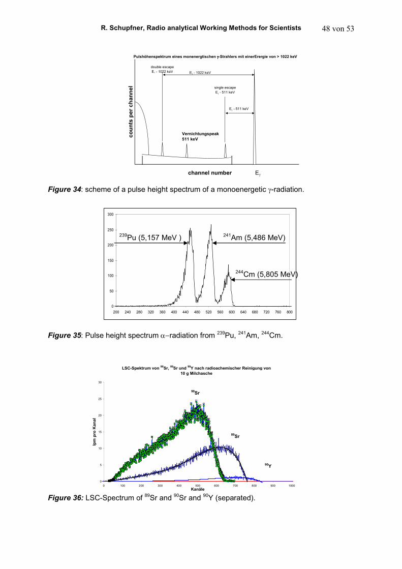
R. Schupfner, Radio analytical Working Methods for Scientists 48 von 53
Figure 34: scheme of a pulse height spectrum of a monoenergetic γ-radiation. Figure 35: Pulse height spectrum α−radiation from 239Pu, 241Am, 244Cm. Figure 36: LSC-Spectrum of 89Sr and 90Sr and 90Y (separated).
0
50
100
150
200
250
300
200 240 280 320 360 400 440 480 520 560 600 640 680 720 760 800
244Cm (5,805 MeV)
channel number Eγ
co
un
ts p
er
ch
an
nel
Pulshöhenspektrum eines monenergtischen γγγγ-Strahlers mit einerErergie von > 1022 keV
Vernichtungspeak
511 keV
single escapeEγ - 511 keV
Eγ - 511 keV
double escapeEγ - 1022 keV Eγ - 1022 keV
241Am (5,486 MeV) 239Pu (5,157 MeV )
LSC-Spektrum von 90
Sr, 89
Sr und 90
Y nach radioachemischer Reinigung von
10 g Milchasche
0
5
10
15
20
25
30
0 100 200 300 400 500 600 700 800 900 1000Kanäle
Ipm
pro
Kan
al
90Sr
90Y
89Sr
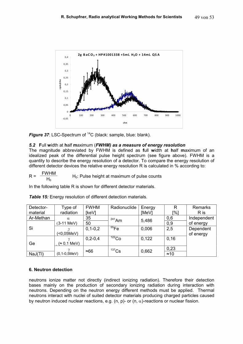
R. Schupfner, Radio analytical Working Methods for Scientists 49 von 53
Figure 37: LSC-Spectrum of 14C (black: sample, blue: blank). 5.2 Full width at half maximum (FWHM) as a measure of energy resolution The magnitude abbreviated by FWHM is defined as full width at half maximum of an idealized peak of the differential pulse height spectrum (see figure above). FWHM is a quantity to describe the energy resolution of a detector. To compare the energy resolution of different detector devices the relative energy resolution R is calculated in % according to: R = H0: Pulse height at maximum of pulse counts In the following table R is shown for different detector materials. Table 15: Energy resolution of different detection materials. Detector-material
Type of radiation
FWHM [keV]
Radionuclide Energy [MeV]
R [%]
Remarks R is
Ar-Methan 35 0,6 α
(3-11 MeV) 50 241Am 5,486
0,9 Independent of energy
Si γ (<0,05MeV)
0,1-0,2 55Fe 0,006 2,5
γ
(≈ 0,1 MeV) 0,2-0,4 122Co 0,122 0,16
Ge 0,23
NaJ(Tl) γ
(0,1-0,5MeV) ≈66 137Cs 0,662 ≈10
Dependent of energy
6. Neutron detection neutrons ionize matter not directly (indirect ionizing radiation). Therefore their detection bases mainly on the production of secondary ionizing radiation during interaction with neutrons. Depending on the neutron energy different methods must be applied. Thermal neutrons interact with nuclei of suited detector materials producing charged particles caused by neutron induced nuclear reactions, e.g. (n, p)- or (n, α)-reactions or nuclear fission.
FWHM H0
2g B aC O 3 + HP #1001338 +5mL H2O + 14mL QS A
-0,05
0
0,05
0,1
0,15
0,2
0,25
0,3
0,35
0,4
0 100 200 300 400 500 600 700 800 900 1000
chn
cp
m/c
hn
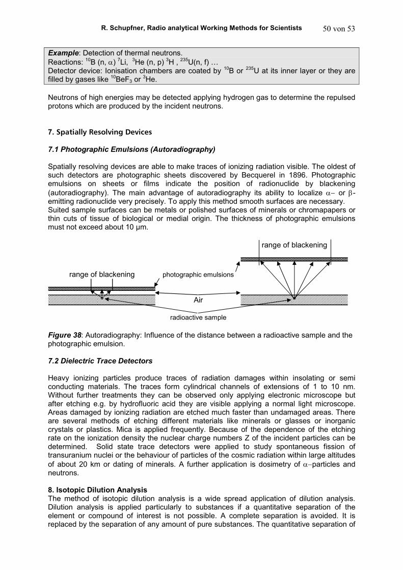
R. Schupfner, Radio analytical Working Methods for Scientists 50 von 53
Example: Detection of thermal neutrons. Reactions: 10B (n, α) 7Li, 3He (n, p) 3H , 235U(n, f) … Detector device: Ionisation chambers are coated by 10B or 235U at its inner layer or they are filled by gases like 10BeF3 or 3He. Neutrons of high energies may be detected applying hydrogen gas to determine the repulsed protons which are produced by the incident neutrons. 7. Spatially Resolving Devices 7.1 Photographic Emulsions (Autoradiography) Spatially resolving devices are able to make traces of ionizing radiation visible. The oldest of such detectors are photographic sheets discovered by Becquerel in 1896. Photographic emulsions on sheets or films indicate the position of radionuclide by blackening (autoradiography). The main advantage of autoradiography its ability to localize α− or β-emitting radionuclide very precisely. To apply this method smooth surfaces are necessary. Suited sample surfaces can be metals or polished surfaces of minerals or chromapapers or thin cuts of tissue of biological or medial origin. The thickness of photographic emulsions must not exceed about 10 µm.
range of blackening
range of blackening
° °Air
photographic emulsions
radioactive sample Figure 38: Autoradiography: Influence of the distance between a radioactive sample and the photographic emulsion. 7.2 Dielectric Trace Detectors Heavy ionizing particles produce traces of radiation damages within insolating or semi conducting materials. The traces form cylindrical channels of extensions of 1 to 10 nm. Without further treatments they can be observed only applying electronic microscope but after etching e.g. by hydrofluoric acid they are visible applying a normal light microscope. Areas damaged by ionizing radiation are etched much faster than undamaged areas. There are several methods of etching different materials like minerals or glasses or inorganic crystals or plastics. Mica is applied frequently. Because of the dependence of the etching rate on the ionization density the nuclear charge numbers Z of the incident particles can be determined. Solid state trace detectors were applied to study spontaneous fission of transuranium nuclei or the behaviour of particles of the cosmic radiation within large altitudes of about 20 km or dating of minerals. A further application is dosimetry of α−particles and neutrons. 8. Isotopic Dilution Analysis The method of isotopic dilution analysis is a wide spread application of dilution analysis. Dilution analysis is applied particularly to substances if a quantitative separation of the element or compound of interest is not possible. A complete separation is avoided. It is replaced by the separation of any amount of pure substances. The quantitative separation of
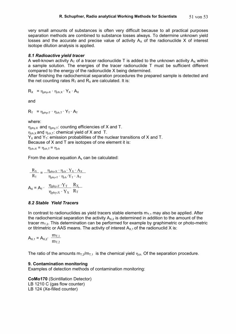
R. Schupfner, Radio analytical Working Methods for Scientists 51 von 53
very small amounts of substances is often very difficult because to all practical purposes separation methods are combined to substance losses always. To determine unknown yield losses and the accurate and precise value of activity AX of the radionuclide X of interest isotope dilution analysis is applied. 8.1 Radioactive yield tracer A well-known activity AT of a tracer radionuclide T is added to the unknown activity AX within a sample solution. The energies of the tracer radionuclide T must be sufficient different compared to the energy of the radionuclide X being determined. After finishing the radiochemical separation procedures the prepared sample is detected and the net counting rates RT and RX are calculated. It is: RX = ηphy,X · ηch,X · YX · AX and RT = ηphy,T · ηch,T · YT · AT where: ηphy,X and ηphy,T: counting efficiencies of X and T. ηch,X and ηch,T: chemical yield of X and T. YX and YT: emission probabilities of the nuclear transitions of X and T. Because of X and T are isotopes of one element it is: ηch,X = ηch,T = ηch From the above equation Ax can be calculated: = AX = AT · · 8.2 Stable Yield Tracers In contrast to radionuclides as yield tracers stable elements mT,1 may also be applied. After the radiochemical separation the activity AX,2 is determined in addition to the amount of the tracer mT,2. This determination can be performed for example by graphimetric or photo-metric or titrimetric or AAS means. The activity of interest AX,1 of the radionuclid X is: AX,1 = AX,2· The ratio of the amounts mT,2/mT,1 is the chemical yield ηch. Of the separation procedure.
9. Contamination monitoring Examples of detection methods of contamination monitoring: CoMo170 (Scintillation Detector) LB 1210 C (gas flow counter) LB 124 (Xe-filled counter)
RX RT
ηphy,X · ηch · YX · AX
ηphy,T · ηch ·YT · AT
ηphy,T ·YT ηphy,X · YX
RX RT
mT,1
mT,2
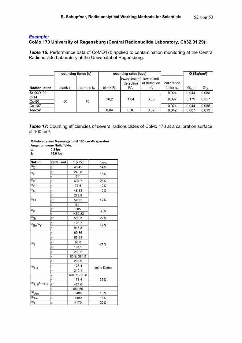
R. Schupfner, Radio analytical Working Methods for Scientists 52 von 53
Example: CoMo 170 University of Regensburg (Central Radionuclide Laboratory, Ch32.01.29): Table 16: Performance data of CoMO170 applied to contamination monitoring at the Central Radionuclide Laboratory at the Universität of Regensburg.
Radionuclide blank t0 sample tM blank R0
lower limit of detection
R*n
lower limit of detection
ρ*n
calibration factor κO OLLD ODL
Sr-90/Y-90 0,024 0,044 0,088C-14Co-60Cs-137 0,024 0,044 0,088Am-241 0,04 0,16 0,32 0,042 0,007 0,013
0,357
counting times [s] counting rates [cps] O Bq/cm²]
0,09760 10
10,2 1,84 3,68 0,179
Table 17: Counting efficiencies of several radionuclides of CoMo 170 at a calibration surface of 100 cm².
Mittelwerte aus Messungen mit 100 cm²-Präparaten
Angenommene Nulleffekte:
α: α: α: α: 0,2 Ips
β: β: β: β: 15,0 Ips
Nuklid Zerfallsart E [keV] ηηηηPhys
14C β− 49,45 14%
β+ 249,8
γ 51132P β
− 694,7 25%33P β
− 76,6 12%35S β
− 48,83 12%
β− 278,8
β+ 59,35
γ 511β
− 585γ 1460,83
89Sr β− 583,3 27%
β− 195,7
β− 943,8
β− 69,35
β− 86,93
β− 96,6
β− 191,5
β− 283,2
γ 80,2; 364,5β
− 23,09
β− 123,4
β− 210,1
γ 604,7; 795,8β
− 173,4 35%
β− 424,6
γ 661,66241Am α 5486 18%238Pu α 5499 18%238U α 4170 22%
42%
21%
keine Daten
18F 18%
137Cs/137mBa
40K
36Cl
90Sr/90Y
131I
134Cs
42%
30%
R. Schupfner, Radio analytical Working Methods for Scientists 53 von 53
Determination of surface contamination applying CoMo170 for the purpose of removing things out of controlled areas For example: threshold of gross counting rate Radionuclide of calibration: 90Sr (in secular equilibrium to 90Y) Conditions: - limit of surface contamination must be known - Calculation of threshold gross counting rate R´threshold t0 = 60 s, tb = 10 s R0 ± ∆R0 ≈ (13,2 ± 2,8) cps at a confidence level of 99% R´threshold ≈ 16 cps O(R´threshold) = κO·R´threshold ≈ 0,4 Bq/cm². Assessment: Comparison to values Olimit of App,. III Table 1 Column 4: 14C, 32P, 33P, 35S: 100 Bq/cm² ⇒ portion O(R´threshold)/Olimit < 0,4 Bq/cm²/100 Bq/cm² < 0,004 125I: 10 Bq/cm² ⇒ portion O(R´threshold)/Olimit < 0,4 Bq/cm²/10 Bq/cm² < 0,04 60Co, 90Sr, 137Cs: 1 Bq/cm² ⇒ portion O(R´threshold)/Olimit < 0,4 Bq/cm²/1 Bq/cm² < 0,4 If the gross counting rate R´ is below R´threshold the thing may removed from the controlled area as far as no α-contamination occurred and the radionuclide mixture contains no low energy β-or ec-emitters.