A Geometric Approach to Statistical Learning Theory...

A Geometric Approach to Statistical Learning

Theory

Shahar Mendelson

Centre for Mathematics and its Applications

The Australian National University

Canberra, Australia

What is a learning problem

• A class of functions F on a probability space (Ω, µ)

• A random variable Y one wishes to estimate

• A loss functional `

• The information we have: a sample (Xi, Yi)ni=1

Our goal: with high probability, find a good approximation to Y in F with

respect to `, that is

• Find f ∈ F such that E`(f (X), Y )) is “almost optimal”.

• f is selected according to the sample (Xi, Yi)ni=1.

Shahar Mendelson: A Geometric Approach to Statistical Learning Theory

Example

Consider

• The random variable Y is a fixed function T : Ω → [0, 1] (that is Yi =

T (Xi)).

• The loss functional is `(u, v) = (u− v)2.

Hence, the goal is to find some f ∈ F for which

E`(f (X), T (X)) = E(f (X)− T (X))2 =

∫Ω

(f (t)− T (t))2dµ(t)

is as small as possible.

To select f we use the sample X1, ..., Xn and the values T (X1), ..., T (Xn).


A variation

Consider the following excess loss:

¯f(x) = (f (x)− T (x))2 − (f ∗(x)− T (x))2 = `f(x)− `f∗(x),

where f ∗ minimizes E`f(x) = E(f (X)− T (X))2 in the class.

The difference between the two cases:


Our Goal

• Given a fixed sample size, how close to the optimal can one get using em-

pirical data?

• How does the specific choice of the loss influence the estimate?

• What parameters of the class F are important?

• Although one has access to a random sample, the measure which generates

the data is not known.


The algorithm

Given a sample (X1, ..., Xn), select f ∈ F which satisfies

argminf∈F

1

n

n∑i=1

`f(Xi),

that is, f is the “best function” in the class on the data.

The hope is that with high probability E(`f |X1, ..., Xn) =∫

`f(t)dµ(t) is close

to the optimal.

In other words, hopefully, with high probability, the empirical minimizer of theloss is “almost” the best function in the class with respect to the loss.


Back to the squared loss

In the case of the squared excess loss -

¯f(x) = (f (x)− T )2 − (f ∗(x)− T (x))2,

since the second term if the same for every f ∈ F , the empirical minimization

selects

argminf∈F

n∑i=1

(f (Xi)− T (Xi))2

and the question is

how to relate this empirical distance to the “real” distance we are interestedin.


Analyzing the algorithm

For a second, let’s forget the loss, and from here on, to simplify notation, denote

by G the loss class.

We shall attempt to connect 1n

∑ni=1 g(Xi) (i.e. the random, empirical structure

on G) to Eg.

We shall examine various notions of similarity of the structures.

Note: in the case of an excess loss, 0 ∈ G and our aim is to be as close to 0 as

possible. Otherwise, our aim is to approach g∗ 6= 0.


A road map

• Asking the “correct” question - beware of loose methods of attack.

• Properties of the loss and their significance.

• Estimating the complexity of a class.


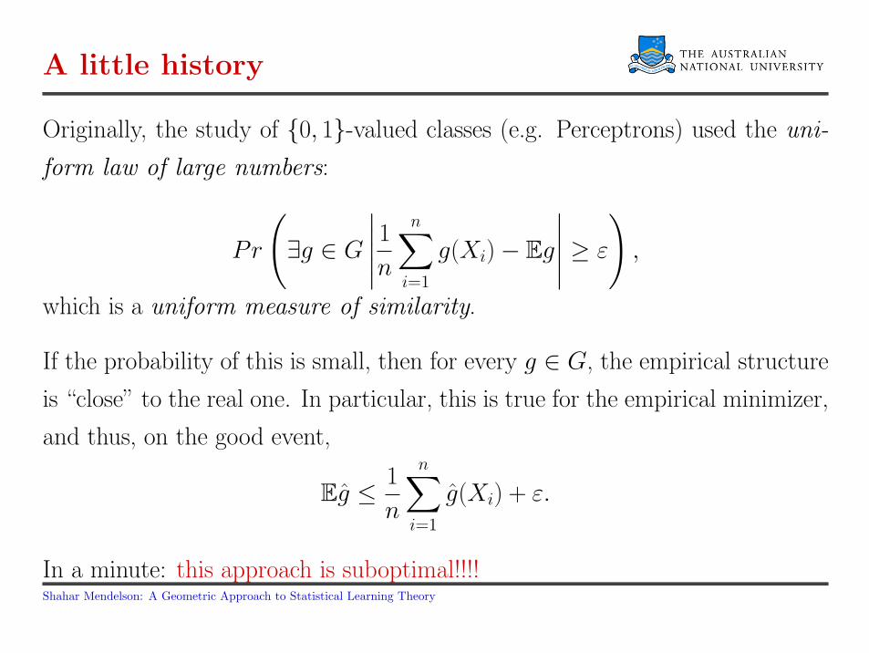
A little history

Originally, the study of 0, 1-valued classes (e.g. Perceptrons) used the uni-

form law of large numbers:

Pr

(∃g ∈ G

∣∣∣∣∣1nn∑

i=1

g(Xi)− Eg

∣∣∣∣∣ ≥ ε

),

which is a uniform measure of similarity.

If the probability of this is small, then for every g ∈ G, the empirical structure

is “close” to the real one. In particular, this is true for the empirical minimizer,

and thus, on the good event,

Eg ≤ 1

n

n∑i=1

g(Xi) + ε.

In a minute: this approach is suboptimal!!!!Shahar Mendelson: A Geometric Approach to Statistical Learning Theory

Why is this bad?

Consider the excess loss case.

• We hope that the algorithm will get us close to 0...

• So, it seems likely that we would only need to control the part of G which

is not too far from 0.

• No need to control functions which are far away, while in the ULLN, we

control every function in G.


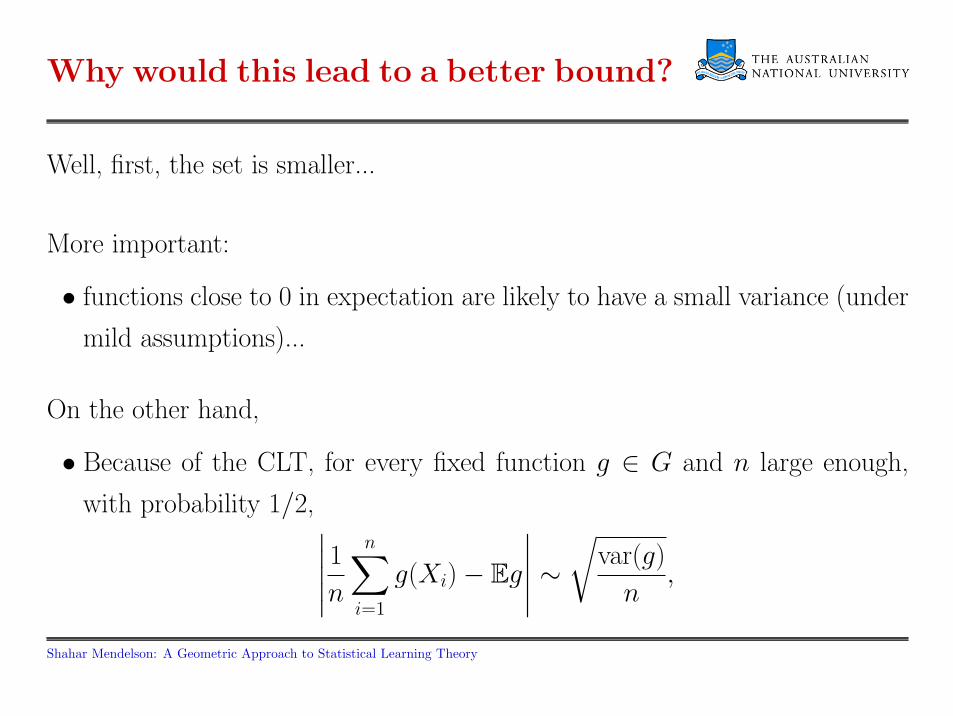
Why would this lead to a better bound?

Well, first, the set is smaller...

More important:

• functions close to 0 in expectation are likely to have a small variance (under

mild assumptions)...

On the other hand,

• Because of the CLT, for every fixed function g ∈ G and n large enough,

with probability 1/2, ∣∣∣∣∣1nn∑

i=1

g(Xi)− Eg

∣∣∣∣∣ ∼√

var(g)

n,


So?

• Control over the entire class =⇒ control over functions with nonzero variance

=⇒ rate of convergence can’t be better than c/√

n.

• If g∗ 6= 0, we can’t hope to get a faster rate than c/√

n using this method.

• This shows the statistical limitation of the loss.


What does this tell us about the loss?

• To get faster convergence rates one has to consider the excess loss.

• We also need a condition that would imply that if the expectation is small,

the variance is small (e.g E`2f ≤ BE`f - A Bernstein condition).

It turns out that this condition is connected to convexity properties of ` at

0.

• One has to connect the richness of G to that of F (which follows from a

Lipshitz condition on `).


Localization - Excess loss

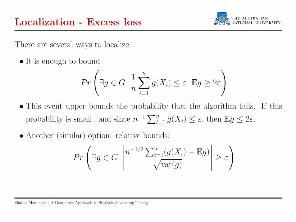
There are several ways to localize.

• It is enough to bound

Pr

(∃g ∈ G

1

n

n∑i=1

g(Xi) ≤ ε Eg ≥ 2ε

)• This event upper bounds the probability that the algorithm fails. If this

probability is small , and since n−1∑n

i=1 g(Xi) ≤ ε, then Eg ≤ 2ε.

• Another (similar) option: relative bounds:

Pr

(∃g ∈ G

∣∣∣∣∣n−1/2∑n

i=1(g(Xi)− Eg)√var(g)

∣∣∣∣∣ ≥ ε

)


Comparing structures

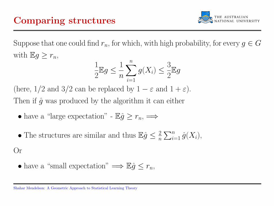
Suppose that one could find rn, for which, with high probability, for every g ∈ G

with Eg ≥ rn,1

2Eg ≤ 1

n

n∑i=1

g(Xi) ≤3

2Eg

(here, 1/2 and 3/2 can be replaced by 1− ε and 1 + ε).

Then if g was produced by the algorithm it can either

• have a “large expectation” - Eg ≥ rn, =⇒

• The structures are similar and thus Eg ≤ 2n

∑ni=1 g(Xi),

Or

• have a “small expectation” =⇒ Eg ≤ rn,


Comparing structures II

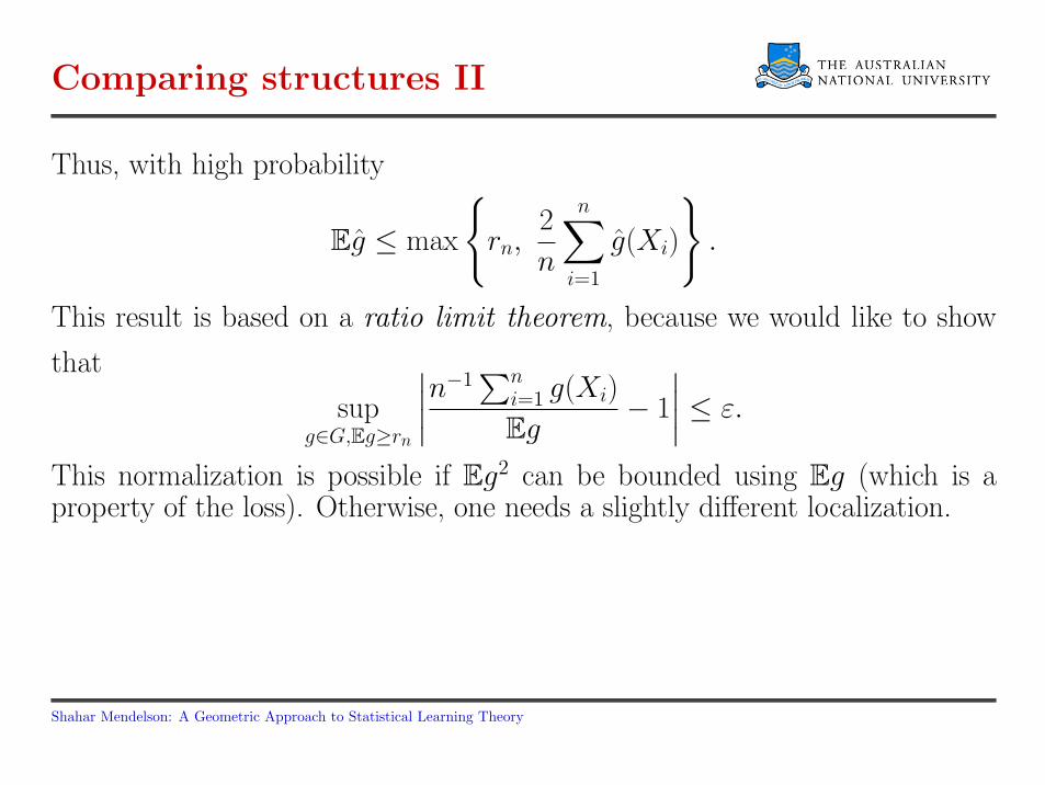
Thus, with high probability

Eg ≤ max

rn,

2

n

n∑i=1

g(Xi)

.

This result is based on a ratio limit theorem, because we would like to show

that

supg∈G,Eg≥rn

∣∣∣∣n−1∑n

i=1 g(Xi)

Eg− 1

∣∣∣∣ ≤ ε.

This normalization is possible if Eg2 can be bounded using Eg (which is aproperty of the loss). Otherwise, one needs a slightly different localization.


Star shape

If G is star-shaped, its “relative richness” increases as r becomes smaller.


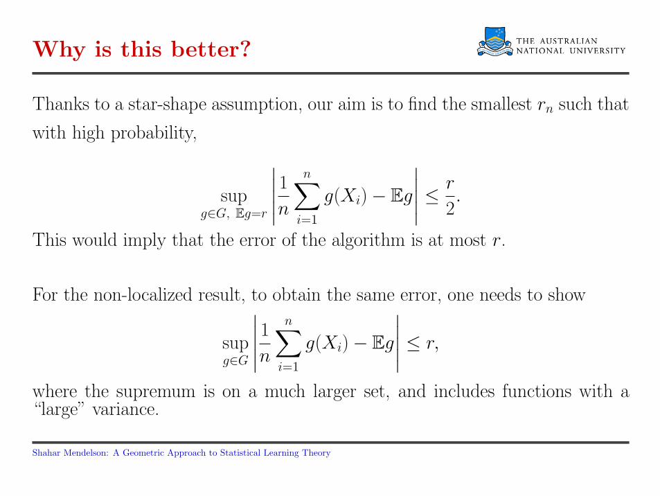
Why is this better?

Thanks to a star-shape assumption, our aim is to find the smallest rn such that

with high probability,

supg∈G, Eg=r

∣∣∣∣∣1nn∑

i=1

g(Xi)− Eg

∣∣∣∣∣ ≤ r

2.

This would imply that the error of the algorithm is at most r.

For the non-localized result, to obtain the same error, one needs to show

supg∈G

∣∣∣∣∣1nn∑

i=1

g(Xi)− Eg

∣∣∣∣∣ ≤ r,

where the supremum is on a much larger set, and includes functions with a“large” variance.


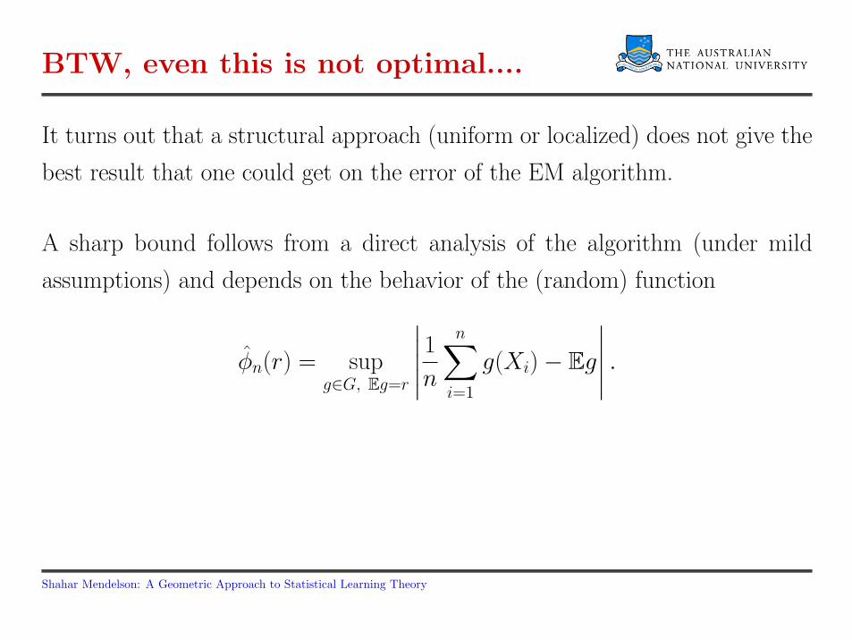
BTW, even this is not optimal....

It turns out that a structural approach (uniform or localized) does not give the

best result that one could get on the error of the EM algorithm.

A sharp bound follows from a direct analysis of the algorithm (under mild

assumptions) and depends on the behavior of the (random) function

φn(r) = supg∈G, Eg=r

∣∣∣∣∣1nn∑

i=1

g(Xi)− Eg

∣∣∣∣∣ .


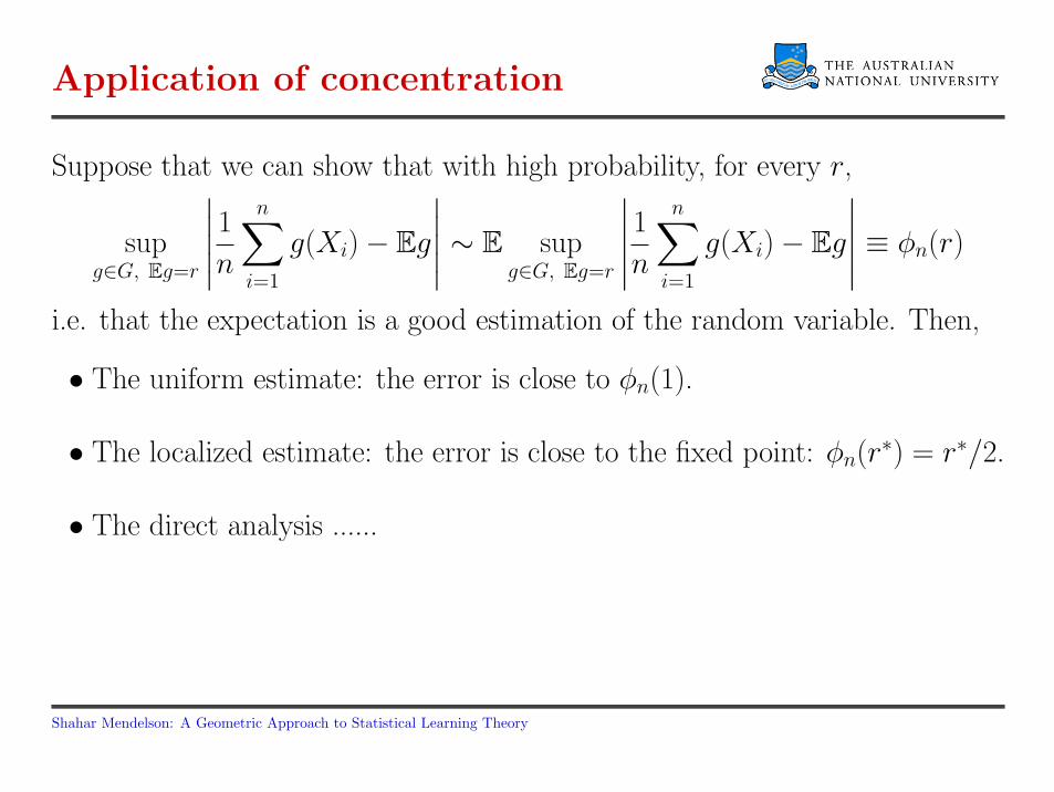
Application of concentration

Suppose that we can show that with high probability, for every r,

supg∈G, Eg=r

∣∣∣∣∣1nn∑

i=1

g(Xi)− Eg

∣∣∣∣∣ ∼ E supg∈G, Eg=r

∣∣∣∣∣1nn∑

i=1

g(Xi)− Eg

∣∣∣∣∣ ≡ φn(r)

i.e. that the expectation is a good estimation of the random variable. Then,

• The uniform estimate: the error is close to φn(1).

• The localized estimate: the error is close to the fixed point: φn(r∗) = r∗/2.

• The direct analysis ......


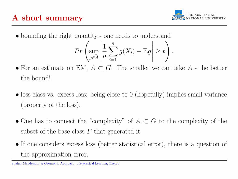
A short summary

• bounding the right quantity - one needs to understand

Pr

(supg∈A

∣∣∣∣∣1nn∑

i=1

g(Xi)− Eg

∣∣∣∣∣ ≥ t

).

• For an estimate on EM, A ⊂ G. The smaller we can take A - the better

the bound!

• loss class vs. excess loss: being close to 0 (hopefully) implies small variance

(property of the loss).

• One has to connect the “complexity” of A ⊂ G to the complexity of the

subset of the base class F that generated it.

• If one considers excess loss (better statistical error), there is a question of

the approximation error.Shahar Mendelson: A Geometric Approach to Statistical Learning Theory

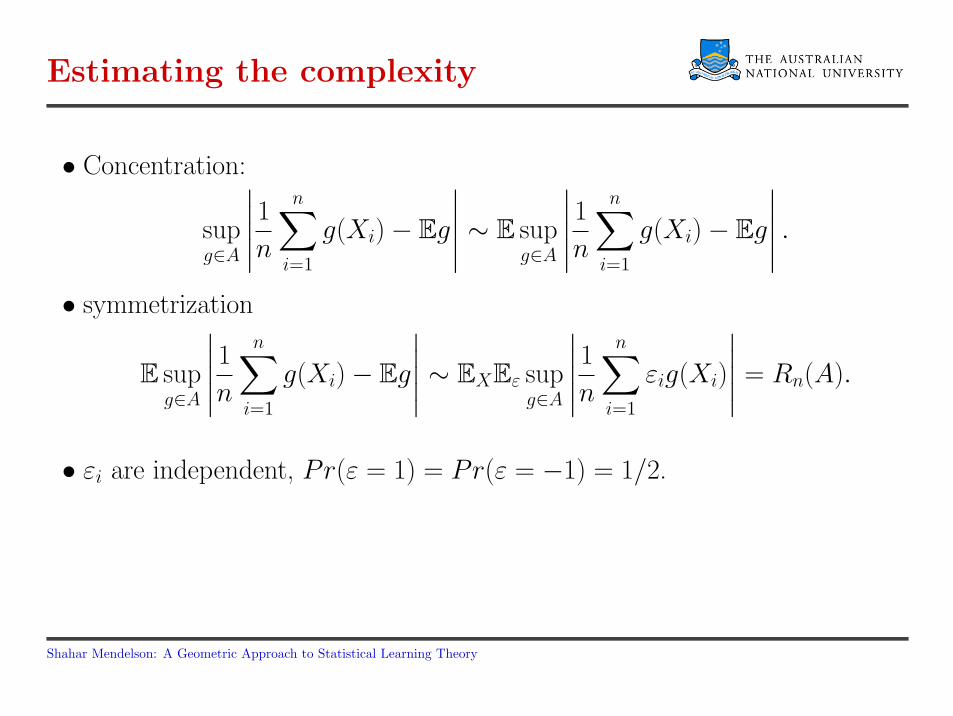
Estimating the complexity

• Concentration:

supg∈A

∣∣∣∣∣1nn∑

i=1

g(Xi)− Eg

∣∣∣∣∣ ∼ E supg∈A

∣∣∣∣∣1nn∑

i=1

g(Xi)− Eg

∣∣∣∣∣ .• symmetrization

E supg∈A

∣∣∣∣∣1nn∑

i=1

g(Xi)− Eg

∣∣∣∣∣ ∼ EXEε supg∈A

∣∣∣∣∣1nn∑

i=1

εig(Xi)

∣∣∣∣∣ = Rn(A).

• εi are independent, Pr(ε = 1) = Pr(ε = −1) = 1/2.


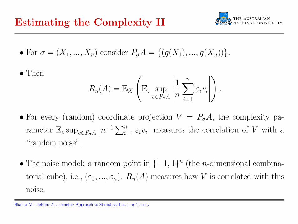
Estimating the Complexity II

• For σ = (X1, ..., Xn) consider PσA = (g(X1), ..., g(Xn)).

• Then

Rn(A) = EX

(Eε sup

v∈PσA

∣∣∣∣∣1nn∑

i=1

εivi

∣∣∣∣∣)

.

• For every (random) coordinate projection V = PσA, the complexity pa-

rameter Eε supv∈PσA

∣∣n−1∑n

i=1 εivi

∣∣ measures the correlation of V with a

“random noise”.

• The noise model: a random point in −1, 1n (the n-dimensional combina-

torial cube), i.e., (ε1, ..., εn). Rn(A) measures how V is correlated with this

noise.


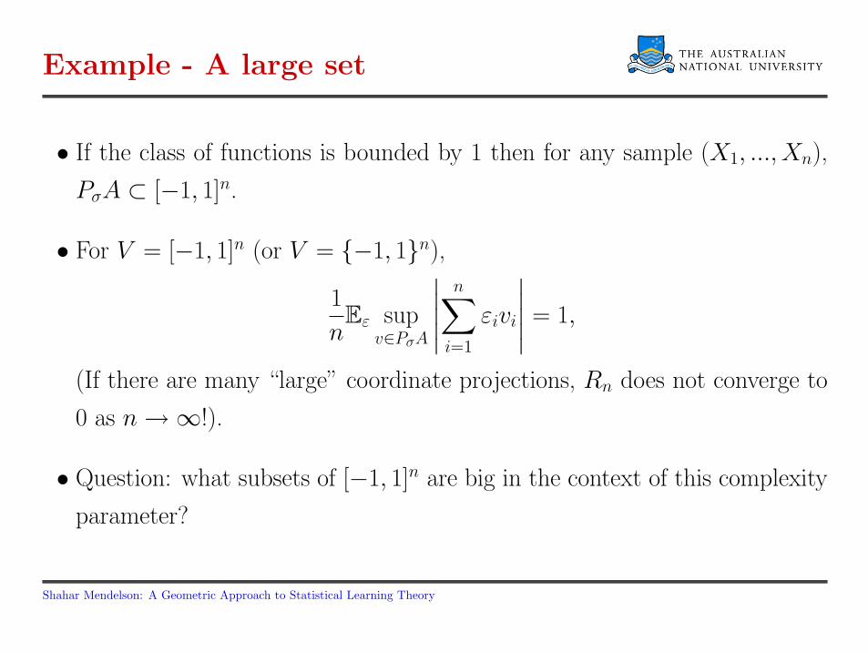
Example - A large set

• If the class of functions is bounded by 1 then for any sample (X1, ..., Xn),

PσA ⊂ [−1, 1]n.

• For V = [−1, 1]n (or V = −1, 1n),

1

nEε sup

v∈PσA

∣∣∣∣∣n∑

i=1

εivi

∣∣∣∣∣ = 1,

(If there are many “large” coordinate projections, Rn does not converge to

0 as n →∞!).

• Question: what subsets of [−1, 1]n are big in the context of this complexity

parameter?


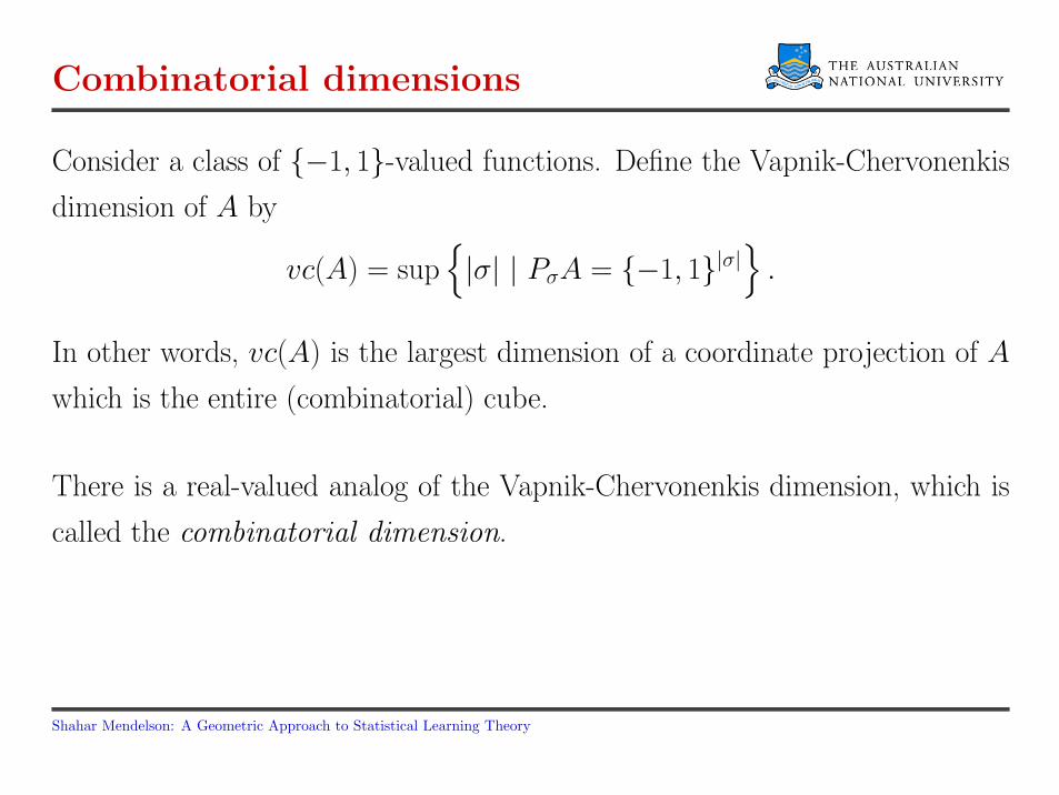
Combinatorial dimensions

Consider a class of −1, 1-valued functions. Define the Vapnik-Chervonenkis

dimension of A by

vc(A) = sup|σ| | PσA = −1, 1|σ|

.

In other words, vc(A) is the largest dimension of a coordinate projection of A

which is the entire (combinatorial) cube.

There is a real-valued analog of the Vapnik-Chervonenkis dimension, which is

called the combinatorial dimension.


Combinatorial dimensions II

The combinatorial dimension:

For every ε, it measures the largest dimension |σ| of a “cube” of side length ε

that can be found in a coordinate projection PσA.


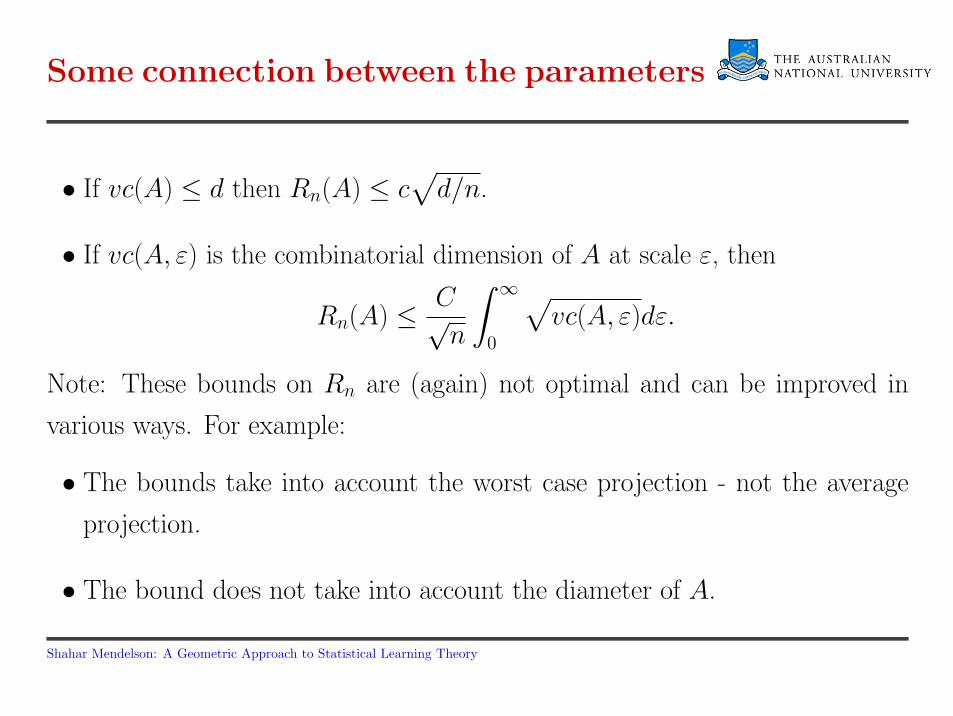
Some connection between the parameters

• If vc(A) ≤ d then Rn(A) ≤ c√

d/n.

• If vc(A, ε) is the combinatorial dimension of A at scale ε, then

Rn(A) ≤ C√n

∫ ∞

0

√vc(A, ε)dε.

Note: These bounds on Rn are (again) not optimal and can be improved in

various ways. For example:

• The bounds take into account the worst case projection - not the average

projection.

• The bound does not take into account the diameter of A.


Important

The vc dimension (combinatorial dimension) and other related complexity pa-

rameters (e.g covering numbers) are only ways of upper bounding Rn.

Sometimes such a bound is good, but at times it is not.

Although the connections between the various complexity parameters are very

interesting and nontrivial, for SLT it is always best to try and bound Rn directly.

Again, the difficulty of the learning problem is captured by the “richness” of a

random coordinate projection of the loss class.


Example: Error rates for VC classes

Let

• F be a class of 0, 1-valued functions with vc(F ) ≤ d and T ∈ F . (Proper

learning)

• ` is the squared loss and G is the loss class. Note, 0 ∈ G!

• H = star(G, 0) = λg | g ∈ G is the star-shaped hull of G.


Example: Error rates for VC classes II

Then:

• Since `f(x) ≥ 0 and functions in F are 0, 1-valued, then Eh2 ≤ Eh.

• The error rate is upper bounded by the fixed point of

E suph∈H, Eh=r

∣∣∣∣∣n−1n∑

i=1

εih(Xi)

∣∣∣∣∣ = Rn(Hr),

i.e. when

Rn(Hr) =r

2.

• The next step is to relate the complexity of Hr to the complexity of F .


Bounding Rn(Hr)

• F is small in the appropriate sense.

• ` is a Lipschitz function, and thus G = `(F ) is not much larger than F .

• The star-shaped hull of G is not much larger than G.

In particular, for every n ≥ d, with probability larger than 1 −(

edn

)c′d, if

Eng ≤ infg∈G Eng + ρ, then

Eg ≤ c max

d

nlog( n

ed

), ρ

.


A Geometric Approach to Statistical Learning Theory...

Documents

Transcript of A Geometric Approach to Statistical Learning Theory...