A -Convergence Result for the Upper Bound Limit Analysis of Platescarlier/gamma_cv.pdf · A...

September 25, 2014 19:29 WSPC/INSTRUCTION FILE gamma˙cv

A Γ-Convergence Result for the Upper Bound

Limit Analysis of Plates

Jeremy BLEYER

Universite Paris-Est, Laboratoire Navier,Ecole des Ponts ParisTech-IFSTTAR-CNRS (UMR 8205), FRANCE

jeremy. bleyer@ enpc. fr

Guillaume CARLIER

CEREMADE,

Universite Paris-Dauphine, FRANCE

carlier@ ceremade. dauphine. fr

Vincent DUVAL

INRIA,

Domaine de Voluceau, Rocquencourt, FRANCE

vincent. duval@ inria. fr

Jean-Marie MIREBEAU and Gabriel PEYRE

CNRS, CEREMADE,Universite Paris-Dauphine, FRANCE

mirebeau,peyre@ ceremade@ ceremade. dauphine. fr

Upper bound limit analysis allows one to evaluate directly the ultimate load of structures

without performing a cumbersome incremental analysis. In order to numerically applythis method to thin plates in bending, several authors have proposed to use various

finite elements discretizations. We provide in this paper a mathematical analysis which

ensures the convergence of the finite element method, even with finite elements withdiscontinuous derivatives such as the quadratic 6 node Lagrange triangles and the cubic

Hermite triangles. More precisely, we prove the Γ-convergence of the discretized problemstowards the continuous limit analysis problem. Numerical results illustrate the relevanceof this analysis for the yield design of both homogeneous and non-homogeneous materials.

Keywords: Bounded Hessian functions; Finite Element Method; Γ-convergence.

AMS Subject Classification: 74K20, 74S05, 74G15

1. Introduction and Motivation of the Model

Yield design or limit analysis theory aims at evaluating directly the ultimate load

of mechanical structures using the compatibility between equilibrium equations and

a local strength criterion. More precisely, assuming that the structure Ω is subject

to a multiplicative loading λL, the ultimate load multiplicative factor λ+ is obtained

1

[email protected]

[email protected]

[email protected]

mirebeau,peyre@[email protected]


2 J. Bleyer, G. Carlier, V. Duval, J.-M. Mirebeau and G. Peyre

by solving the following formal problem

λ+ = maxλ∈R,Σ∈S

λ s.t. ∀x ∈ Ω,

E(Σ)(x) = λL(x),

Σ(x) ∈ G(x),

where Σ(x) represents the internal forces at a point x of the structure Ω and where

S collects all fields Σ of internal forces which satisfy the stress boundary conditions,

E is a linear differential operator corresponding to the equilibrium equations and

G(x) is a convex set representing the strength criterion at a point x in the structure

Ω. This means that the ultimate load represents the greatest load factor such that

there exists at least one field of internal forces in the structure satisfying both the

equilibrium equation and the strength criterion at each point.

The dual problem can be expressed formally as follows :

λ+ = minu∈C

∫Ω

π(x,Du)dx s.t.

∫Ω

L(x)u(x)dx = 1 (1.1)

where D = E∗ is the dual equilibrium operator or the strain operator, u is a virtual

velocity field which has to satisfy the velocity boundary conditions and π(x, ·) is

the support function of G(x). This dual formulation means that the ultimate load

corresponds to the minimum of the maximal resisting work over all virtual velocity

fields satisfying a normalization condition on the work of external forces. Both

approaches, the primal one (known as the static approach) and the dual one (known

as the kinematical approach), are equivalent and can be implemented numerically

by an appropriate discretization of the stress or velocity fields, yielding to a lower

bound or an upper bound of the ultimate load factor.

In this work, we are interested in the kinematical approach (1.1) with virtual

velocity fields for a specific mechanical model, namely the thin plate model. In this

model, Ω is a region of R2 and the internal forces are the bending moments and

are represented by a symmetric matrix field M(x) (see [CD79] for the derivation of

this model). The equilibrium operator is a second-order operator namely E(M) =

div divM . For this reason, the strain rate (or curvature rate for the plate model) is

given by the Hessian matrix of the scalar velocity field u as κ = Du = D2u.

1.1. Previous Works

Numerical limit analysis of thin plate in bending problems. From a nu-

merical point of view, the resolution of such limit analysis problems is traditionally

performed by discretizing the structure into finite elements while the correspond-

ing discrete variational inequality problem is formulated as a convex programming

problem. Early works considered a linear interpolation of the velocity in each tri-

angular finite element [MDF78]. The corresponding mathematical problem can be

formulated as a linear programming problem and can be solved using simplex or

interior-point algorithms. This very simple discretization is known as the yield line

method in the field of plate mechanics, since each finite element admits a potential

discontinuity of the velocity gradient (corresponding to the plate rotation) along its


A Γ-Convergence Result for the Upper Bound Limit Analysis of Plates 3

edges. In particular, no curvature deformation occurs inside any element since the

Hessian is identically zero. Therefore, this method fails in general to predict the ex-

act collapse load even with an infinitely refined mesh as pointed out by Braestrup

[Bræ71], the computed upper bound being then very sensitive to the mesh lay-

out [Joh94, Jen96]. Hodge and Belytschko considered a quadratic interpolation of

the velocity field ensuring only C0 continuity between elements [HJB68] whereas

later works used C1-continuous elements [CC99, LNXND10]. More recently, it was

suggested in [BdB13] that the use of finite elements ensuring C0 continuity only

exhibits better convergence rates to the exact collapse load than elements ensuring

C1-continuity. Finally, one can also mention recent papers relying on a meshfree

discretization [LGA09, ZLC12].

Mathematical models and their analysis. The function π appearing in the

limit analysis problem (1.1) having linear growth and the strain operator D be-

ing of second order, the adequate functional space for the study of (1.1) is the

space of bounded Hessian functions, which consists of functions whose second deriva-

tive is a bounded Radon measure. This space was introduced and studied in the

pioneering work of Demengel and Temam [Dem83, Dem84, Tem85, Dem89]: the

abstract properties of bounded Hessian functions are established in [Dem84] (see

also [Tem85]), whereas [Dem83] studies the limit analysis problem in the homoge-

neous case (π(x,Du) = Π(Du)): existence of solutions and their characterization are

stated. Compactness properties are studied in [Dem89] with an application to the

limit load problem. Finer mechanical models may also involve the space of bounded

Hessian functions: in [Had85b, Had88], it is used together with the space of bounded

deformations to model the bending and the compression of a plate constituted by

an elastoplastic material.

The strain Du being a Radon measure, it raises the issue of the definition of∫Ωπ(x,Du)dx as a convex function of a measure, which was tackled in [DT84] in

the case of a uniform penalty π (independent of x) and in [Had85a] in the general

case. This extended formulation allows to deal with inhomogeneous penalties as

in [Had86]. Eventually Telega studies in [Tel95] the case of a periodically inhomo-

geneous plate material, and he shows the Γ-convergence of the problem towards

the homogeneous problem as the period vanishes (see below for the definition of

Γ-convergence).

1.2. Contributions and Outline of the Paper

This work is a companion paper to the numerical study [BdB13]. We consider a

relaxed formulation of (1.1) (similar relaxations are shown to be tight in [Dem83]

in the study of the homogeneous case),

infu∈HB(Ω)

∫Ω

π(x,D2u

)+

∫ΓN

π

(x,−∂u

∂νν ⊗ ν

)dH1 (1.2)



where ΓN ⊆ ∂Ω, and we impose the constraint that u = 0 on ΓD ⊆ ∂Ω and that the

load L should satisfy 〈L, u〉 = 1. The precise definitions of each notion is given in

Section 2. As for∫

Ωπ(x,D2u

), we rely on a formulation due to Reshetnyak which

is different from [Had85a] and which is exposed in [AFP00]. Its main advantage is

that it provides continuity properties provided π is continuous in the first variable.

Our main contribution is to ensure the consistency of the finite element method

used in [BdB13] to solve (1.2). We prove that the discretized problems Γ-

converge towards Problem (1.2) as the size of the triangulation goes to

zero. As a consequence every cluster point (which always exists) of the solutions

to the discrete problems is a solution to (1.2).

To our knowledge, although Γ-convergence results of finite element approxima-

tions exist in the literature for first order strain/equilibrium operators (e.g. [BDH89,

OP11]), this kind of issue has never been tackled for the second-order operators in-

volved in the thin plate limit analysis. Such a problem raises specific issues like the

use of the space of bounded Hessian functions, (i.e. whose second derivative is a

Radon measure) as opposed to the classical Sobolev spaces W 1,p or W 2,p, p > 1.

The outline of the paper is as follows. In Section 2, several facts about the

space of functions with bounded Hessian are recalled. The hypotheses about the

domain and the penalty function π are stated precisely. The formulation of the

continuous problem is given in Section 3. For the sake of completeness, we give a

proof of existence of solutions, although the argument is similar to the one used

by Demengel [Dem83] for the homogeneous case. We also state an approximation

result of functions with bounded Hessian with functions which are C3 up to the

boundary. The main result of the paper is stated in Section 4, where we describe

the finite element approximations and we prove their Γ-convergence towards the

continuous problem. Eventually, Section 5 provides numerical experiments which

illustrate the efficiency of the approximation including in both the homogeneous

(constant π) and the inhomogeneous cases.

Notations. We adopt the following definitions and notations throughout the pa-

per.

E2 is the set of real symmetric tensors of order 2. For A,B ∈ E2, their double

inner product is A :B =∑

16i,j62AijBij . The Frobenius norm of A ∈ E2 defined

by |A|F =√A :A is denoted by |A|F or simply |A|.

We denote by L2 the Lebesgue measure on R2, by H1 the one-dimensional

Hausdorff measure. Given a Borel set B ⊆ R2, H1 xB refers to the restriction of

H1 to B, that is (H1 xB)(E) = H1(B∩E) for all E ⊆ R2. More generally, we write

(µ xB)(E) = µ(B ∩E) for any Borel measure µ and any µ-measurable set E ∈ R2.

Given a finite dimensional vector space X, Mb(Ω, X) will denote the set of finite

X-valued Radon measures on the open set Ω. For all sets E ⊂ Ω, E⊂⊂Ω means

that its closure E is compact and E ⊂ Ω.

Given a locally integrable function u : Ω→ R, we denote by Du (resp. D2u) its



x1

x2

x3

x4x5

ΓD

ΓN

Ω

Ω

Ω

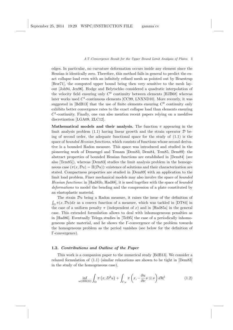
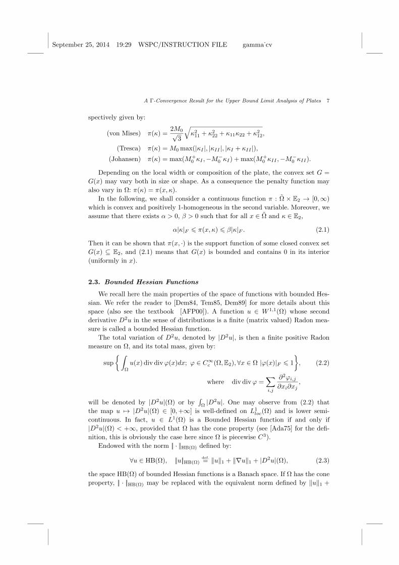
Fig. 1: The domain Ω is piecewise C3 regular, i.e. C3 except at a finite number

of points x1, . . . xJ. The (relaxed) Neumann boundary condition is imposed on

ΓN = (∂Ω) ∩ Ω where Ω ⊃ Ω is a piecewise C3 domain.

distributional derivative (resp. second derivative). If Du is representable by some

locally integrable function (i.e. u has a Sobolev regularity), we refer to it as ∇u.

A similar convention is adopted for D2u and ∇2u. The restriction of u to some set

B ⊆ R2 is denoted by u|B .

Given a real vector space X and a function q : X → [−∞,+∞], we say that q

is positively 1-homogeneous if for all x ∈ X, and all t > 0 q(tx) = tq(x).

Eventually, Pk denotes the space of polynomials of two variables of degree k or

less and SN−1 denotes the unit sphere of RN .

2. Preliminaries

2.1. Domain Regularity and Boundary Conditions

Throughout this paper, we shall consider a piecewise C3-regular domain Ω ⊂ R2.

More precisely, we assume that Ω ⊂ R2 is a bounded connected open set and there

exists a finite set x1, . . . , xJ ⊆ ∂Ω such that

• for all x ∈ ∂Ω \ x1, . . . , xJ, ∂Ω is C3 regular in a neighborhood of x,

• there exist pairwise disjoint open neighborhoods Vj of xj , for each j ∈1, . . . , J and C3-diffeomorphisms ϕj from Vj to (−1, 1)2 such that

ϕj(xj) = (0, 0)

ϕj(Vj ∩ Ω) = (0, 1)2.

In the last section, when studying the convergence of the finite element approxima-

tion, we shall make the stronger assumption that Ω is a convex polytope.

As for the boundary conditions imposed to Problem (1.2), we shall assume

that the Dirichlet condition u = 0 (or more precisely γ0u = 0, see the definition

in Section 2.3) is imposed on ΓD, where ΓD is a union of connected components

of ∂Ω \ x1, . . . , xJ. Moreover, the Neumann boundary condition ∂u∂ν = 0 (in fact

γ1u = 0, see below) is imposed on ΓN , where ΓN is a union of connected components



of ∂Ω\x1, . . . , xJ such that ΓN ⊆ ΓD. Observe that we work in fact with a relaxed

Neumann condition, as shown in the formulation (1.2).

From the above assumptions, we deduce that there exists a bounded open

connected set Ω ⊆ R2 with piecewise smooth boundary such that Ω ⊂ Ω and

ΓN = (∂Ω) ∩ Ω (modulo the points (xj)16j6J , see Figure 1).

Eventually, we assume that ΓD contains at least three points which are not

aligned.

2.2. The Penalty Function π

The mechanical strength of the plate is described by a closed convex set G ⊂ E2

such that any bending state outside of G is impossible to achieve whereas a bending

state lying on the boundary of G means that the plate attained its full strength

capacity at this given point. For thin plates in bending, the convex set G is supposed

to be bounded and to contain 0. Typical examples of such criteria are the following:

• the von Mises criterion: it is characterized by a mechanical parameter M0 >

0 which represents the plate strength in uniaxial bending and it is given by

the following quadratic norm on the components Mij of M :

G = M ∈ E2 |√M2

11 +M222 −M11M22 + 3M2

12 6M0

• the Tresca criterion: it is also characterized by a parameter M0 having the

same mechanical interpretation but here the criterion is expressed in terms

of the eigenvalues MI and MII of the bending moment M so that it is

different from the von Mises criterion:

G = M ∈ E2 | max(|MI |, |MII |, |MI −MII |) 6M0

• the Johansen criterion: it can be characterized by two parameters

M+0 ,M

−0 > 0 which represent the plate strength in positive and negative

uniaxial bending and it is given by:

G = M ∈ E2 | −M−0 6MI ,MII 6M+0

We refer the reader to [Pra59] for more details about the physical concepts involved

in the limit analysis of thin plates.

It is equivalent to specify G or to specify its support function π (see [Roc83])

which appears naturally in the kinematical approach:

π(κ) = supM : κ , M ∈ G.

It can be shown that π is convex continuous and positively homogeneous. The

support functions corresponding to the previous classical strength criteria are re-



spectively given by:

(von Mises) π(κ) =2M0√

3

√κ2

11 + κ222 + κ11κ22 + κ2

12,

(Tresca) π(κ) = M0 max(|κI |, |κII |, |κI + κII |),(Johansen) π(κ) = max(M+

0 κI ,−M−0 κI) + max(M+

0 κII ,−M−0 κII).

Depending on the local width or composition of the plate, the convex set G =

G(x) may vary both in size or shape. As a consequence the penalty function may

also vary in Ω: π(κ) = π(x, κ).

In the following, we shall consider a continuous function π : Ω × E2 → [0,∞)

which is convex and positively 1-homogeneous in the second variable. Moreover, we

assume that there exists α > 0, β > 0 such that for all x ∈ Ω and κ ∈ E2,

α|κ|F 6 π(x, κ) 6 β|κ|F . (2.1)

Then it can be shown that π(x, ·) is the support function of some closed convex set

G(x) ⊆ E2, and (2.1) means that G(x) is bounded and contains 0 in its interior

(uniformly in x).

2.3. Bounded Hessian Functions

We recall here the main properties of the space of functions with bounded Hes-

sian. We refer the reader to [Dem84, Tem85, Dem89] for more details about this

space (also see the textbook [AFP00]). A function u ∈ W 1,1(Ω) whose second

derivative D2u in the sense of distributions is a finite (matrix valued) Radon mea-

sure is called a bounded Hessian function.

The total variation of D2u, denoted by |D2u|, is then a finite positive Radon

measure on Ω, and its total mass, given by:

sup

∫Ω

u(x) div divϕ(x)dx; ϕ ∈ C∞c (Ω,E2),∀x ∈ Ω |ϕ(x)|F 6 1

, (2.2)

where div divϕ =∑i,j

∂2ϕi,j∂xi∂xj

,

will be denoted by |D2u|(Ω) or by∫

Ω|D2u|. One may observe from (2.2) that

the map u 7→ |D2u|(Ω) ∈ [0,+∞] is well-defined on L1loc(Ω) and is lower semi-

continuous. In fact, u ∈ L1(Ω) is a Bounded Hessian function if and only if

|D2u|(Ω) < +∞, provided that Ω has the cone property (see [Ada75] for the defi-

nition, this is obviously the case here since Ω is piecewise C3).

Endowed with the norm || · ||HB(Ω) defined by:

∀u ∈ HB(Ω), ||u||HB(Ω)def.= ‖u‖1 + ‖∇u‖1 + |D2u|(Ω), (2.3)

the space HB(Ω) of bounded Hessian functions is a Banach space. If Ω has the cone

property, || · ||HB(Ω) may be replaced with the equivalent norm defined by ‖u‖1 +



|D2u|(Ω) for all u ∈ HB(Ω) (see [Dem84, Prop. 1.3]), and the injection HB(Ω) →W 1,1(Ω) is compact. Moreover, the injection HB(Ω) → C(Ω) is continuous.

Two other topologies, known as the “weak” and “intermediate” topologies, are

introduced in [Dem84]. The weak topology is the one induced by the norm || · ||W 1,1

and the family of seminorms u 7→∣∣∫

Ωψd(D2u)ij

∣∣ for all ψ ∈ C∞c (Ω) and 1 6 i, j 62. Here, (D2u)ij refers to each entry of D2u, so that it is a signed Radon measure,

and in fact∫

Ωψd(D2u)ij =

∫Ωu(x)

∂2ϕi,j

∂xi∂xj(x)dx. An important property is that if a

sequence of functions (un)n∈N is bounded in HB(Ω) (for the strong topology), then

there exists a function u∞ ∈ HB(Ω) and a subsequence (un′)n′∈N that converges

towards u∞ for the weak topology.

The intermediate topology is defined by the distance

d(u1, u2)def.= ‖u1 − u2‖1 +

∣∣|D2u1|(Ω)− |D2u2|(Ω)∣∣ . (2.4)

Although it is not completely obvious, the intermediate topology is finer than

the weak topology, as shown in the next proposition.

Proposition 1. Let u ∈ HB(Ω) and (un)n∈N ∈ (HB(Ω))N such that

limn→+∞

d(u, un) = 0.

Then un converges towards u for the HB(Ω)-weak topology.

Proof. The main point to prove is that limn→+∞ ‖∇(u− un)‖L1 = 0.

Assume by contradiction that there is some ε > 0 and a subsequence (still de-

noted un) such that ‖∇(un − u)‖L1 > ε. The sequence ‖un‖L1 + |D2un|(Ω) being

bounded (so that ‖un‖HB(Ω) is bounded as well, by equivalence of the norms) we

may extract a subsequence which converges in W 1,1(Ω) towards some u ∈ HB(Ω).

In particular we have limn→+∞ ‖∇(un − u)‖L1 = 0. Since on the other hand

limn→+∞ ‖un−u‖L1 = 0, we must have u = u, and thus limn→+∞ ‖∇(un−u)‖L1 =

0, which contradicts the assumption. Thus limn→+∞ ‖∇(u− un)‖L1 = 0.

The weak-* convergence of D2un towards D2u comes from the fact that

limn→+∞ un = u in L1(Ω) and that supn∈N(|D2un|(Ω)

)< +∞.

The following important result of Demengel states that any function in HB(Ω)

may be approximated by smooth functions.

Proposition 2 ([Dem84, Prop. 1.4]). For all u ∈ HB(Ω), there exists a sequence

un ∈ C∞(Ω) ∩W 2,1(Ω) such that limn→+∞ d(un, u) = 0.

It is possible to define the trace of a bounded Hessian function, and the normal

trace of its gradient: there exists continuous (for the strong topology) linear opera-

tors γ0 : HB(Ω) → W 1,1(Γ) and γ1 : HB(Ω) → L1(Γ) such that for all u ∈ C2(Ω),

γ0(u) = u|Γ and γ1(u) = ∂u∂ν |Γ (where ν is the outer unit normal to Ω). It turns

out that γ0 and γ1 are continuous w.r.t. the intermediate topology defined by (2.4).

For the sake of simplicity, for u ∈ HB(Ω) and when the context is clear, we shall



sometimes write u|Γ (resp. ∂u∂ν |Γ) instead of γ0(u) (resp. γ1(u)). It is worth noting

that one may require in Proposition 2 (see [Dem84]) that the approximating se-

quence (un)n∈N should consist of smooth functions which have the same traces as

u: γ0un = γ0u, γ1un = γ1u for all n ∈ N.

Eventually, we shall rely on the following gluing theorem proved by Demen-

gel [Dem84] (see also [AFP00, Corollary 3.89]). Let U , V ⊂ R2 be two open sets

with Lipschitz boundary such that U ⊂ V , and let Γ = V ∩ ∂U . For u ∈ HB(U),

v ∈ HB(V \ U) define

w =

u in U,

v in V \ U.

Theorem 2.1 ([Dem84]). The function w is in HB(V ) if and only if γ0u = γ0v

on Γ, and then

D2w = (D2u) xU + (D2v) x (V \ U) +

(∂v

∂ν− ∂u

∂ν

)ν ⊗ ν H1 xΓ, (2.5)

where ν is the normal from U to V \ U .

2.4. Functionals Involving the Hessian

2.4.1. Convex Function of a Measure

In this paragraph, we recall some results about convex functionals of a measure.

We refer the reader to [AFP00, Section 2.6] for a detailed exposition on this notion.

We consider a Borel function f : Ω × RN → [0,∞) (where N ∈ N∗ and Ω is

defined in Section 2.1), positively 1-homogeneous and convex in the second vari-

able. Given any bounded Radon measure µ ∈ Mb(Ω,RN ), µ is absolutely con-

tinuous w.r.t. its total variation |µ| and the Radon-Nikodym derivative µ|µ| is a

|µ|-measurable function (such that µ|µ| (x) ∈ SN−1 for |µ|-almost every x ∈ Ω). Thus

we may define

J(µ)def.=

∫Ω

f

(x,

µ

|µ|(x)

)d|µ|(x). (2.6)

One may show that J is convex, positively 1-homogeneous, and that J(µ1 + µ2) =

J(µ1)+J(µ2) when the measures µ1 and µ2 are mutually singular. Moreover, a result

by Reshetnyak [AFP00, Th. 2.38] ensures that it is weak-* lower semi-continuous

provided f : Ω × RN → [0,∞] is lower semi-continuous. More precisely, if µn ∈Mb(Ω,RN ) and µn

∗ µ ∈Mb(Ω,RN ), then

J(µ) 6 lim infn→+∞

J(µn). (2.7)

If additionally the restriction of f to Ω×SN−1 is continuous and bounded, and that

|µn|(Ω)→ |µ|(Ω), Reshetnyak’s continuity theorem ([AFP00, Th. 2.39]) states that

J(µ) = limn→+∞

J(µn). (2.8)



2.4.2. Energy with Boundary Terms

Now we assume that π satisfies the hypotheses of Section 2.2. From Theorem 2.1,

we know that we may extend any function u ∈ HB(Ω) such that γ0u = 0 in ΓDinto a function u ∈ HB(Ω) such that u = 0 in Ω \ Ω. Combining this observation

with the framework of Section 2.4.1, we define its energy as∫

Ωπ(x, D

2u|D2u| (x))|D2u|,

which turns out to be

J(u) =

∫Ω

π

(x,

D2u

|D2u|(x)

)|D2u|+

∫ΓN

π

(x,−∂u

∂νν ⊗ ν

)dH1(x). (2.9)

The next two propositions describe the (lower semi-)continuity properties of J

with respect to the topologies of HB(Ω).

Proposition 3. The functional J : HB(Ω) → [0,∞) is sequentially lower semi-

continuous for the weak topology of HB(Ω) (or the L1(Ω) strong topology).

Proof. Let (un)n∈N ∈ (HB(Ω))N which converges towards some u ∈ HB(Ω) for the

weak topology (or the L1(Ω) strong topology). We want to prove that

lim infn→+∞

J(un) > J(u).

Recall that J(u) =∫

Ωπ(x, D

2u|D2u| (x)

)|D2u|, where u is extended as the null function

on Ω \ Ω. However we cannot directly apply Reshetnyak’s lower semi-continuity

theorem since the sequence (D2un) does not a priori converge towards D2u for the

weak-* topology of Mb(Ω).

Let l = lim infn→+∞ J(un). If l = +∞, there is nothing to prove. Assuming that

l < +∞, we extract a subsequence un′ such that limn→∞ J(un′) = l. Then for n′

large enough,

α|D2un′ |(Ω) = α

(|D2un′ |(Ω) +

∫ΓN

∣∣∣∣∂un′

∂ν

∣∣∣∣ dH1

)6 J(un′) 6 l + 1. (2.10)

Since un′ converges towards u in L1(Ω), we obtain that D2un converges towards

D2u for the weak-* topology of Mb(Ω). By Reshetnyak’s lower semi-continuity

theorem [AFP00, Th. 2.38], we obtain the desired inequality.

Proposition 4. The functional J : HB(Ω)→ [0,∞) is continuous for the interme-

diate topology of HB(Ω).

Proof. Let (un)n∈N ∈ (HB(Ω))N be a sequence such that limn→∞ d(u, un) = 0,

where d is the distance defining the intermediate topology of Ω (see (2.4)).

By continuity of the trace γ1 with respect to the intermediate topology,

limn→+∞ γ1un = γ1u in L1(∂Ω), so that

|D2un|(Ω) +

∫ΓN

∣∣∣∣∂un∂ν∣∣∣∣ dH1 → |D2u|(Ω) +

∫ΓN

∣∣∣∣∂u∂ν∣∣∣∣ dH1,



or equivalenty, considering the extension of u to Ω described above,

|D2un|(Ω)→ |D2u|(Ω).

Moreover, since limn→+∞ un = u in L1(Ω), we see that D2un∗ D2u in Mb(Ω).

By Reshetnyak’s continuity theorem [AFP00, Th. 2.39] we obtain that

limn→+∞

∫Ω

π

(x,

D2un|D2un|

)|D2un| =

∫Ω

π

(x,

D2u

|D2u|

)|D2u|,

which is the desired result.

3. The Continuous Problem in HB(Ω)

3.1. Formulation of the Problem

From now on, we consider Ω, ΓD, ΓN and π which satisfy the hypotheses of Sec-

tion 2, and we assume that we are given a load, that is a linear form L : HB(Ω)→ Rsuch that either L is continuous with respect to the weak topology defined in Sec-

tion 2.3 or its restriction to bounded subsets of HB(Ω) is (sequentially) continuous

for the weak topology. This holds if for instance one of the three conditions hold:

• L ∈ (W 1,1(Ω))′,

• L is the second derivative of a continuous function with compact support

in Ω, e.g. L = div divM for some M ∈ Cc(Ω,E2),

• L is a measure which does not charge horizontal and vertical lines,

or if L is a linear combination of such linear forms.

Remark 3.1. It is important to observe that not all measures µ ∈ Mb(Ω) are

continuous for the HB(Ω) weak topology. In [Dem89], the author has exhibited

a bounded sequence of functions un which converges to 0 for the HB(Ω) weak

topology but such that 〈δx0, un〉 = 1 for all n ∈ N (where δx0

is the Dirac mass at

some x0 ∈ Ω).

The continuity of L in the first two cases is straightforward, let us give some

details on the last case. Let L be a finite measure which does not charge horizontal

and vertical lines (in the sense that neither its positive nor negative part does) and

un converge weakly in HB(Ω) to some u and such that ‖un‖HB(Ω) is bounded. We

claim then that 〈L, un〉 converges to 〈L, u〉. Proceeding as in [Dem84], by suitable

extension arguments, we may assume that un are HB in the whole plane with (a

common) compact support. We then have (see [Dem84]) supn ‖un‖L∞ 6 C and

un(x, y) = θn(Qx,y), u(x, y) = θ(Qx,y)

where θn and θ are the measures of mixed second partial derivatives

θndef.=

∂2un∂x∂y

, θdef.=

∂2u

∂x∂y, Qx,y

def.= (−∞, x]× (−∞, y].



By assumption θn converges weakly ∗ to θ, but since |θn| is bounded, we may also

assume, taking a subsequence if necessary, that |θn| converges weakly ∗ to some

measure µ (with µ ≥ |θ|). There exists two subsets of R, I and J which are at most

countable and for which as soon as x ∈ R \ I and y ∈ R \ J one has:

µ(∂Qx,y) = 0. (3.1)

Now we claim that, as soon as x ∈ R\I and y ∈ R\J , un(x, y) converges to u(x, y).

Indeed, let ε > 0 and ϕε ∈ C(R2, [0, 1]) vanishing outside Qx,y and equal to 1 on

Qεx,y := (−∞, x− ε)× (−∞, y − ε), we then have for every ε > 0:

lim supn|un(x, y)− u(x, y)| ≤ lim sup

n|〈θn − θ, ϕε〉|

+ lim supn|θn|(Qx,y \Qεx,y) + |θ|(Qx,y \Qεx,y)

≤ 2µ(Qx,y \Qεx,y)

where the last line follows from the weak ∗ convergence of θn to θ, the fact that

(Qx,y \Qεx,y) is closed and the inequality µ ≥ |θ|. We then let ε tend to 0 and use

(3.1) to deduce that un(x, y) converges to u(x, y). This proves that un converges to

u |L|-a.e., and together with the L∞ bound and Lebesgue’s dominated convergence

theorem, this yields the claimed convergence.

Remark 3.2. Because of the coercivity of J , all the sequences considered in this

paper shall be bounded in HB(Ω). Therefore, in the following, we shall often refer

to the “continuity of L for the weak topology”, tacitly meaning that the given

argument also holds for loads L such that their restrictions to bounded subsets of

HB(Ω) are continuous for the weak topology.

We also assume that there exists a function u ∈ HB(Ω) such that u|ΓD= 0 and

〈L, u〉 6= 0.

The problem we want to solve is:

infu∈HB(Ω)

J(u) such that

u = 0 on ΓD〈L, u〉 = 1

(LA)

where J(u) =

∫Ω

π

(x,

D2u

|D2u|(x)

)|D2u|+

∫ΓN

π

(x,−∂u

∂νν ⊗ ν

)dH1.

We may also write (LA) as the problem of minimizing the functional F over

HB(Ω), where

F (u)def.=

J(u) if uΓD

= 0 and 〈L, u〉 = 1,

+∞ otherwise.(3.2)

3.2. Existence of a Minimizer

We obtain the existence of a minimizer to (LA) by the direct method of the

calculus of variations.



Proposition 5 (Existence of a minimizer). There exists a solution u? ∈ HB(Ω)

to Problem (LA).

Proof. Let (un)n∈N ∈ HB(Ω)N be any minimizing sequence. Problem (LA) is fea-

sible since there exists u such that u|ΓD= 0 and 〈L, u〉 6= 0. Hence there exists

M ∈ (0,+∞) such that for all n ∈ N, 0 6 J(un) 6M . This implies by the coerciv-

ity of the functional (see Lemma 1 below) that ||un||HB(Ω) is bounded.

Therefore, we may extract a subsequence (un′)n′∈N which converges to some

u? ∈ HB(Ω) for the weak topology. From the continuity of the trace operator γ0 :

W 1,1(Ω) → L1(∂Ω), we obtain that u? = 0 on ΓD. Moreover, from the continuity

of L for the weak topology, 〈L, u?〉 = 1. By Proposition 3 we obtain J(u?) 6lim infn′→+∞ J(un′) = infu∈HB(Ω) F (u).

Hence u? is a solution to Problem (LA).

In the above proof, we have used the coercivity of J with respect to the HB(Ω)

norm. This is a consequence of the following Lemma.

Lemma 1 (Coercivity). There exists C > 0 (which depends only on Ω, π and

ΓD) such that for all u ∈ HB(Ω) with u = 0 on ΓD:

J(u) > C||u||HB(Ω) = C(‖u‖W 1,1 + |D2u|(Ω)

). (3.3)

Proof. We follow the standard proof of the Poincare inequality (see [AFP00]).

Assume by contradition that (3.3) does not hold. Then there exists a sequence

(un)n∈N ∈ (HB(Ω))N, such that for all n ∈ N, γ0un = 0 on ΓD and

α

∫Ω

|D2un| 6∫

Ω

π

(x,

D2un|D2un|

)|D2un| <

1

n‖un‖HB(Ω). (3.4)

Since ||un||HB(Ω) 6= 0, we may assume, up to a rescaling, that ||un||HB(Ω) = 1 so that

the sequence is bounded in HB(Ω).

Hence (see Section 2.3), we may extract a subsequence (un′)n′∈N which weakly

converges to some u ∈ HB(Ω). Since weak convergence in HB(Ω) implies strong

convergence in W 1,1(Ω) we have γ0u = 0 on ΓD. By the lower semi-continuity of

the second variation,

0 6 α

∫Ω

|D2u| 6 lim infn′→+∞

α

∫Ω

|D2un′ | = 0,

so that u ∈ P1. Since ΓD contains three points which are not aligned, this implies

that u = 0, which contradicts limn′→+∞ ||un′ ||HB(Ω) = 1, hence the claimed result.

3.3. An Approximation Result

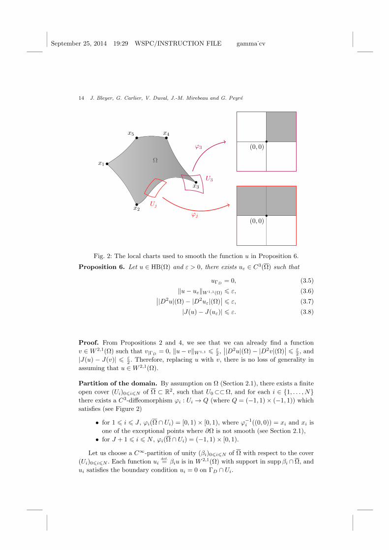
We shall rely on the following result in order to prove the Γ-convergence of the

finite element method.



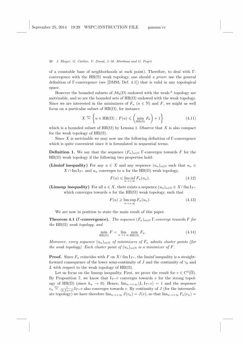
x1

x2

x3

x4x5

Ω

ϕ3

U3

ϕj

Uj

(0, 0)

(0, 0)

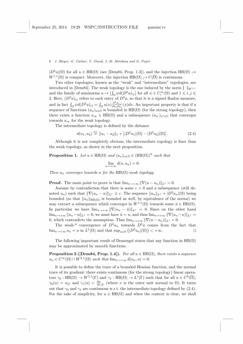
Fig. 2: The local charts used to smooth the function u in Proposition 6.

Proposition 6. Let u ∈ HB(Ω) and ε > 0, there exists uε ∈ C3(Ω) such that

uΓD= 0, (3.5)

‖u− uε‖W 1,1(Ω) 6 ε, (3.6)∣∣|D2u|(Ω)− |D2uε|(Ω)∣∣ 6 ε, (3.7)

|J(u)− J(uε)| 6 ε. (3.8)

Proof. From Propositions 2 and 4, we see that we can already find a function

v ∈W 2,1(Ω) such that v|ΓD= 0, ‖u− v‖W 1,1 6 ε

2 ,∣∣|D2u|(Ω)− |D2v|(Ω)

∣∣ 6 ε2 , and

|J(u) − J(v)| 6 ε2 . Therefore, replacing u with v, there is no loss of generality in

assuming that u ∈W 2,1(Ω).

Partition of the domain. By assumption on Ω (Section 2.1), there exists a finite

open cover (Ui)06i6N of Ω ⊂ R2, such that U0⊂⊂Ω, and for each i ∈ 1, . . . , Nthere exists a C3-diffeomorphism ϕi : Ui → Q (where Q = (−1, 1)× (−1, 1)) which

satisfies (see Figure 2)

• for 1 6 i 6 J , ϕi(Ω ∩ Ui) = [0, 1)× [0, 1), where ϕ−1i ((0, 0)) = xi and xi is

one of the exceptional points where ∂Ω is not smooth (see Section 2.1),

• for J + 1 6 i 6 N , ϕi(Ω ∩ Ui) = (−1, 1)× [0, 1).

Let us choose a C∞-partition of unity (βi)06i6N of Ω with respect to the cover

(Ui)06i6N . Each function uidef.= βiu is in W 2,1(Ω) with support in suppβi ∩Ω, and

ui satisfies the boundary condition ui = 0 on ΓD ∩ Ui.



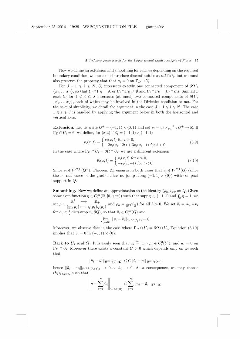
Now we define an extension and smoothing for each ui depending on the required

boundary condition: we must not introduce discontinuities at ∂Ω∩Ui, but we must

also preserve the property that that ui = 0 on ΓD ∩ Ui.For J + 1 6 i 6 N , Ui intersects exactly one connected component of ∂Ω \

x1, . . . xJ, so that Ui ∩ΓD = ∅, or Ui ∩ΓD 6= ∅ and Ui ∩ΓD = Ui ∩ ∂Ω. Similarly,

each Ui for 1 6 i 6 J intersects (at most) two connected components of ∂Ω \x1, . . . xJ, each of which may be involved in the Dirichlet condition or not. For

the sake of simplicity, we detail the argument in the case J + 1 6 i 6 N . The case

1 6 i 6 J is handled by applying the argument below in both the horizontal and

vertical axes.

Extension. Let us write Q+ = (−1, 1)× (0, 1) and set vi = ui ϕ−1i : Q+ → R. If

ΓD ∩ Ui = ∅, we define, for (x, t) ∈ Q = (−1, 1)× (−1, 1)

vi(x, t) =

vi(x, t) for t > 0,

−2vi(x,−2t) + 3vi(x,−t) for t < 0.(3.9)

In the case where ΓD ∩ Ui = ∂Ω ∩ Ui, we use a different extension:

vi(x, t) =

vi(x, t) for t > 0,

−vi(x,−t) for t < 0.(3.10)

Since vi ∈ W 2,1 (Q+), Theorem 2.1 ensures in both cases that vi ∈ W 2,1(Q) (since

the normal trace of the gradient has no jump along (−1, 1) × 0) with compact

support in Q.

Smoothing. Now we define an approximation to the identity (ρh)h>0 on Q. Given

some even function η ∈ C∞c (R, [0,+∞)) such that supp η ⊂ (−1, 1) and∫R η = 1, we

set ρ :R2 −→ R+

(y1, y2) 7−→ η(y1)η(y2)and ρh = 1

h2 ρ( ·h ) for all h > 0. We set vi = ρhi ∗ vi

for hi <12 dist(supp vi, ∂Q), so that vi ∈ C∞c (Q) and

limhi→0+

‖vi − vi‖W 2,1(Q+) = 0.

Moreover, we observe that in the case where ΓD ∩ Ui = ∂Ω ∩ Ui, Equation (3.10)

implies that vi = 0 in (−1, 1)× 0.

Back to Ui and Ω. It is easily seen that uidef.= vi ϕi ∈ C3

c (Ui), and ui = 0 on

ΓD ∩ Ui. Moreover there exists a constant C > 0 which depends only on ϕi such

that

‖ui − ui‖W 2,1(Ui∩Ω) 6 C‖vi − vi‖W 2,1(Q+),

hence ‖ui − ui‖W 2,1(Ui∩Ω) → 0 as hi → 0. As a consequence, we may choose

(hi)16i6N such that∥∥∥∥∥u−N∑i=1

ui

∥∥∥∥∥W 2,1(Ω)

6N∑i=1

‖ui − ui‖W 2,1(Ω)



is arbitrarily small. The function∑Ni=1 ui is in C3(Ω), and by Proposition 4, we

obtain the claimed inequalities.

4. Finite Elements Discretization

This section is devoted to the analysis of the finite element method for Prob-

lem (LA). We refer to [BS08] for a comprehensive exposition of the theory of finite

elements.

4.1. Notations and Definitions

From now on, we assume that Ω ⊂ R2 is a bounded convex polyhedral open set

(which implies the assumptions of Section 2.1. We say that T is a triangulation of

Ω, if it is a finite collection of open triangles Ti such that

• Ti ∩ Tj = ∅ for i 6= j,

•⋃Ti = Ω,

and no vertex of any triangle lies in the interior of an edge of another triangle.

We consider a family of triangulations of Ω, T n, n ∈ N such that there exists

a decreasing sequence (hn)n∈N ∈ RN, such that limn→+∞ hn = 0 and

max diamT ; T ∈ T n 6 hn diam Ω. (4.1)

We say that the family is nondegenerate if there exists ρ > 0 such that for all n ∈ Nand T ∈ T n,

diamBT > ρdiamT (4.2)

where BT is the largest ball contained in T .

Given a triangulation T = T n for some n ∈ N and k ∈ N, the finite element

method consists in defining a global interpolant IT : Ck(Ω) → RΩ which coincides

with some local interpolant IT on each triangle T ∈ T : (IT u)|Tdef.= ITu. We describe

below the finite elements and the corresponding local interpolants used in this paper.

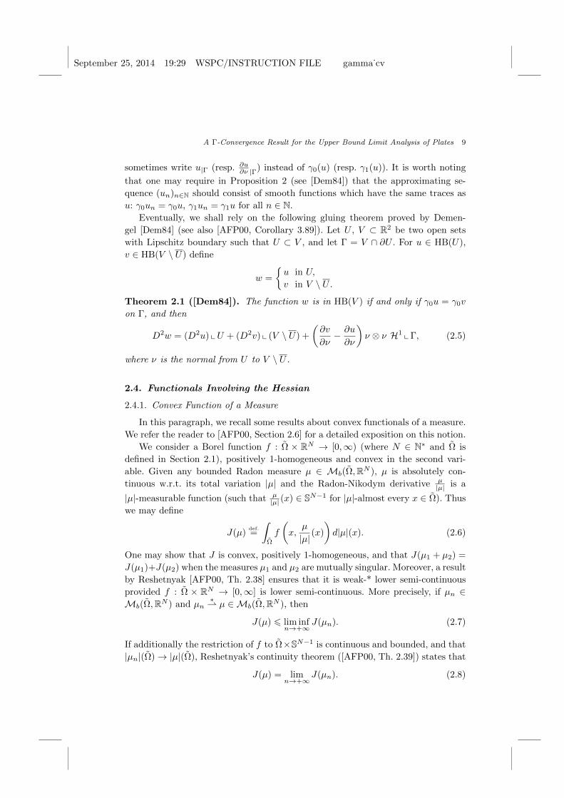
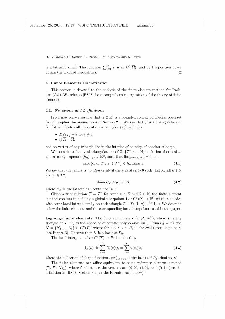
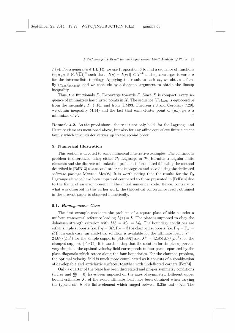
Lagrange finite elements. The finite elements are (T,P2,NT ), where T is any

triangle of T , P2 is the space of quadratic polynomials on T (dimP2 = 6) and

N = N1, . . . N6 ⊂ C0(T )′ where for 1 6 i 6 6, Ni is the evaluation at point zi(see Figure 3). Observe that N is a basis of P ′2.

The local interpolant IT : C0(T )→ P2 is defined by

IT (u)def.=

6∑i=1

Ni(u)ψi =

6∑i=1

u(zi)ψi (4.3)

where the collection of shape functions (ψi)16i66 is the basis (of P2) dual to N .

The finite elements are affine-equivalent to some reference element denoted

(T0,P2,NT0), where for instance the vertices are (0, 0), (1, 0), and (0, 1) (see the

definition in [BS08, Section 3.4] or the Hermite case below).



z0,1 z0,2

z0,3

z0,4

z0,5z0,6

T0

z1z2

z3

z4

z5z6

T

A

Fig. 3: The Lagrange P2 interpolation is determined by 6 control nodes which impose

the values of the polynomial at z1, . . . z6. Those nodes are the three vertices and

the middle of each edge. Each element T is the image of the reference element T0

through some affine map A.

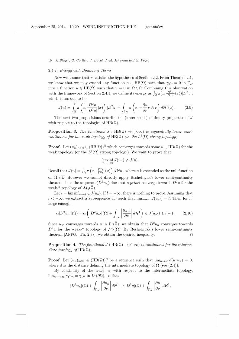
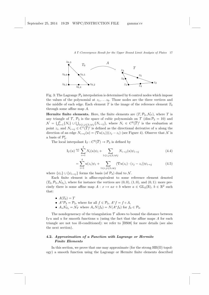
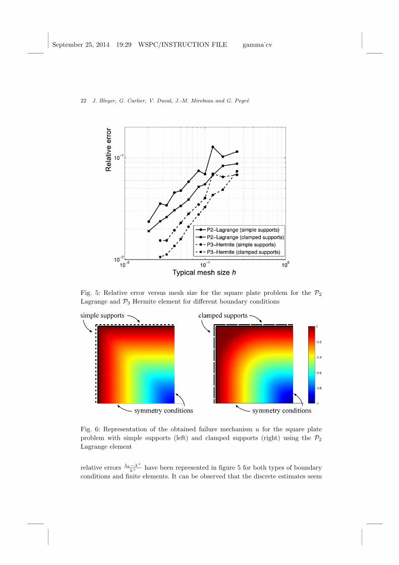
Hermite finite elements. Here, the finite elements are (T,P3,NT ), where T is

any triangle of T , P3 is the space of cubic polynomials on T (dimP3 = 10) and

N =⋃4i=1Ni ∪

⋃16i,j63,i6=jNi→j, where Ni ∈ C0(T )′ is the evaluation at

point zi, and Ni→j ∈ C1(T )′ is defined as the directional derivative of u along the

direction of an edge Ni→j(u) = (∇u(zi))(zj − zi) (see Figure 4). Observe that N is

a basis of P ′3.

The local interpolant IT : C0(T )→ P3 is defined by

IT (u)def.=

4∑i=1

Ni(u)ψi +∑

16i,j63,i6=j

Ni→j(u)ψi→j (4.4)

=

4∑i=1

u(zi)ψi +∑

16i,j63,i6=j

(∇u(zi) · (zj − zi))ψi→j (4.5)

where ψi ∪ ψi→j forms the basis (of P3) dual to N .

Each finite element is affine-equivalent to some reference element denoted

(T0,P3,NT0), where for instance the vertices are (0, 0), (1, 0), and (0, 1): more pre-

cisely there is some affine map A : x 7→ ax + b where a ∈ GL2(R), b ∈ R2 such

that:

• A(T0) = T

• A∗P3 = P3, where for all f ∈ P3, A∗f = f A,

• A∗NT0 = NT where A∗N(f0) = N(A∗f0) for f0 ∈ P3.

The nondegeneracy of the triangulation T allows to bound the distance between

IT u and u for smooth functions u (using the fact that the affine maps A for each

triangle are not too ill-conditioned): we refer to [BS08] for more details (see also

the next section).

4.2. Approximation of a Function with Lagrange or Hermite

Finite Elements

In this section, we prove that one may approximate (for the strong HB(Ω) topol-

ogy) a smooth function using the Lagrange or Hermite finite elements described



z0,1 z0,2

z0,3

z0,4

T0

z1z2

z3

z4

T

A

Fig. 4: The Hermite P3 interpolation is determined by 4 control nodes which impose

the values of the polynomial at z1, . . . z4 and the gradient at z1, z2, z3. Those nodes

are the three vertices and the barycenter. Each element T is the image of the

reference element T0 through some affine map A.

above. As mentioned above, we assume that the family T n, n ∈ N is nondegener-

ate.

Proposition 7. Let u ∈ C3(Ω,R). Then, there exists a constant C > 0 (which only

depends on ρ and Ω), such that for all n ∈ N and T def.= T n .

‖u− IT u‖W 1,1(Ω) 6 C|Ω|h2‖∇3u‖L∞(Ω), (4.6)

|D2u−D2IT u|(Ω) 6 C|Ω|h‖∇3u‖L∞(Ω), (4.7)

where hdef.= hn is the real number given in (4.1).

Proof. In the following, C is a positive constant which may change from one line

to another. We apply [BS08, Corollary 4.4.7] with m = 3, l = 2 (though in fact our

nodal variables only depend on zero and first-order derivatives) and p = +∞: for

0 6 i 6 2 and for each triangle T ⊂ R2, there exists constants Ciγ,δ > 0 such that ,

‖∇iu−∇iITu‖L∞(T ) 6 Ciγ,σ(diamT )3−i‖∇3u‖L∞(T ). (4.8)

The regularity constant Ciγ,δ actually only depends on two characteristics of

the triangle defined in [BS08]: its chunkiness γ = γ(T ), and a Lebesgue constant

σ = σ(T ). These two quantities depend continuously on the triangle shape, and are

scaling and translation invariant.

Given a triangle T , consider T = 1diamT T + bT with bT ∈ R2 chosen so that

T is centered at the origin. The set of all triangles T with diameter 1 such that

(4.2) holds and which are centered at the origin being compact (see the proof of

Theorem 4.4.20 in [BS08]), we obtain that γ(T ) (= γ(T )) and σ(T ) (= σ(T )) are

bounded. Hence Ciγ,σ is bounded as well, which implies that there exists a uniform

constant C > 0 such that for all n ∈ N and T ∈ T n,

‖∇iu−∇iITu‖L∞(T ) 6 C(diamT )3−i‖∇3u‖L∞(T ). (4.9)

Now, let us prove (4.7). We have

|D2u−D2IT u|(Ω) =∑T∈T

∫T

|∇2u(x)−∇2IT u(x)|dx+∑e∈E

∫e

|J∇IT u · νK| dH1.



On the one hand, using (4.9),∫T

|∇2u(x)−∇2IT u(x)|dx 6 |T |‖∇2u−∇2ITu‖L∞(T )

6 |T |C(diamT )‖∇3u‖L∞(T )

6 |T |Ch‖∇3u‖L∞(Ω).

On the other hand, if one edge is shared between triangles S and T :∫e

|J∇IT u · νK| dH1 6 |e|‖∇(ISu− ITu)‖L∞(e)

6 |e|(‖∇(u− ITu)‖L∞(e) + ‖∇(u− ISu)‖L∞(e)

).

By (4.9), since |e| 6 hdiam Ω and (diamT )2 6 1ρ2

(diamBT

diam Ω

)26 C ′|T |:

|e|‖∇(u− ITu)‖L∞(e) 6 |e|C(diamT )2‖∇3u‖L∞(T )

6 hC|T |‖∇3u‖L∞(Ω).

Summing the contributions of triangles and their edges, we obtain (4.7). Equa-

tion (4.6) is obtained in a similar but simpler way, since there is no contribution of

edges.

4.3. Γ-Convergence of the Finite Element Approximation

Let (T n)n∈N be a nondegenerate family of subdivisions of Ω and IT n the corre-

sponding interpolation operator (see Section 4.1). We consider a family of discrete

problems defined by restricting (LA) to the elements of Im IT n :

infu∈HB(Ω)

J(u) such that

u = 0 on ΓD〈L, u〉 = 1,

u ∈ Im IT n .

(LAn)

We may also write (LAn) as the minimization of Fn, where for all u ∈ HB(Ω),

Fn(u)def.=

J(u) if uΓD

= 0, 〈L, u〉 = 1 and u ∈ Im IT n ,

+∞ otherwise.(4.10)

We assume that the triangulation T 0 is coarser than every triangulation T n (n ∈ N),

i.e. the set of edges and nodes of T 0 is included in those of T n. Moreover we

assume that the problem (LA0) is feasible. Then we have of course minHB(Ω) Fn 6minHB(Ω) F0 < +∞.

Our goal is to prove that the minimizers of (LAn) are close to minimizers of (LA)

as the triangulation becomes thin (n→ +∞ so that hn → 0). To this aim we prove

the Γ-convergence of those problems towards (LA). We refer the reader to [DM93,

Bra02] for further details on Γ-convergence.

Remark 4.1. The space HB(Ω) endowed with the weak topology is a topological

vector space which does not satisfy the first axiom of countability (i.e. the existence



of a countable base of neighborhoods at each point). Therefore, to deal with Γ-

convergence with the HB(Ω) weak topology, one should a priori use the general

definition of Γ-convergence (see [DM93, Def. 4.1]) that is valid in any topological

space.

However the bounded subsets of Mb(Ω) endowed with the weak-* topology are

metrizable, and so are the bounded sets of HB(Ω) endowed with the weak topology.

Since we are interested in the minimizers of Fn (n ∈ N) and F , we might as well

focus on a particular subset of HB(Ω), for instance

Xdef.=

u ∈ HB(Ω) ; F (u) 6

(min

HB(Ω)F0

)+ 1

(4.11)

which is a bounded subset of HB(Ω) by Lemma 1. Observe that X is also compact

for the weak topology of HB(Ω).

Since X is metrizable we may now use the following definition of Γ-convergence

which is quite convenient since it is formulated in sequential terms.

Definition 1. We say that the sequence (Fn)n∈N Γ-converges towards F for the

HB(Ω) weak topology if the following two properties hold:

(Liminf inequality) For any u ∈ X and any sequence (un)n∈N such that un ∈X ∩ Im IT n and un converges to u for the HB(Ω) weak topology,

F (u) 6 lim infn→+∞

Fn(un). (4.12)

(Limsup inequality) For all u ∈ X, there exists a sequence (un)n∈N ∈ X∩Im IT n

which converges towards u for the HB(Ω) weak topology, such that

F (u) > lim supn→+∞

Fn(un). (4.13)

We are now in position to state the main result of this paper.

Theorem 4.1 (Γ-convergence). The sequence (Fn)n∈N Γ-converge towards F for

the HB(Ω) weak topology, and

minHB(Ω)

F = limn→+∞

minHB(Ω)

Fn. (4.14)

Moreover, every sequence (un)n∈N of minimizers of Fn admits cluster points (for

the weak topology). Each cluster point of (un)n∈N is a minimizer of F .

Proof. Since Fn coincides with F on X∩Im IT n , the liminf inequality is a straight-

forward consequence of the lower semi-continuity of J and the continuity of γ0 and

L with respect to the weak topology of HB(Ω).

Let us focus on the limsup inequality. First, we prove the result for v ∈ C3(Ω).

By Proposition 7, we know that IT nv converges towards v for the strong topol-

ogy of HB(Ω) (since hn → 0). Hence, limn→+∞〈L, IT nv〉 = 1 and the sequence

vndef.= 1〈L,IT nv〉 IT nv also converges towards v. By continuity of J (for the intermedi-

ate topology) we have therefore limn→+∞ J(vn) = J(v), so that limn→+∞ Fn(vn) =



F (v). For a general u ∈ HB(Ω), we use Proposition 6 to find a sequence of functions

(vk)k∈N ∈ (C3(Ω))N such that |J(u) − J(vk)| 6 2−k and vk converges towards u

for the intermediate topology. Applying the result to each vk, we obtain a fam-

ily (vk,n)(k,n)∈N2 and we conclude by a diagonal argument to obtain the limsup

inequality.

Thus, the functionals Fn Γ-converge towards F . Since X is compact, every se-

quence of minimizers has cluster points in X. The sequence (Fn)n∈N is equicoercive

from the inequality F 6 Fn, and from [DM93, Theorem 7.8 and Corollary 7.20],

we obtain inequality (4.14) and the fact that each cluster point of (un)n∈N is a

minimizer of F .

Remark 4.2. As the proof shows, the result not only holds for the Lagrange and

Hermite elements mentioned above, but also for any affine equivalent finite element

family which involves derivatives up to the second order.

5. Numerical Illustration

This section is devoted to some numerical illustrative examples. The continuous

problem is discretized using either P2 Lagrange or P3 Hermite triangular finite

elements and the discrete minimization problem is formulated following the method

described in [BdB13] as a second-order conic program and solved using the dedicated

software package Mosek [Mos08]. It is worth noting that the results for the P2

Lagrange element have been improved compared to those presented in [BdB13] due

to the fixing of an error present in the initial numerical code. Hence, contrary to

what was observed in this earlier work, the theoretical convergence result obtained

in the present paper is observed numerically.

5.1. Homogeneous Case

The first example considers the problem of a square plate of side a under a

uniform transversal reference loading L(x) = L. The plate is supposed to obey the

Johansen strength criterion with M+0 = M−0 = M0. The boundary conditions are

either simple supports (i.e. ΓD = ∂Ω, ΓN = ∅) or clamped supports (i.e. ΓD = ΓN =

∂Ω). In each case, an analytical solution is available for the ultimate load : λ+ =

24M0/(La2) for the simple supports [SMdS97] and λ+ = 42.851M0/(La

2) for the

clamped supports [Fox74]. It is worth noting that the solution for simple supports is

very simple as the optimal velocity field corresponds to four parts separated by the

plate diagonals which rotate along the four boundaries. For the clamped problem,

the optimal velocity field is much more complicated as it consists of a combination

of developable and anticlastic surfaces, together with undeflected corners [Fox74].

Only a quarter of the plate has been discretized and proper symmetry conditions

(u free and ∂u∂ν = 0) have been imposed on the axes of symmetry. Different upper

bound estimates λh of the exact ultimate load have been obtained when varying

the typical size h of a finite element which ranged between 0.25a and 0.02a. The



Fig. 5: Relative error versus mesh size for the square plate problem for the P2

Lagrange and P3 Hermite element for different boundary conditions

Fig. 6: Representation of the obtained failure mechanism u for the square plate

problem with simple supports (left) and clamped supports (right) using the P2

Lagrange element

relative errors λh−λ+

λ+ have been represented in figure 5 for both types of boundary

conditions and finite elements. It can be observed that the discrete estimates seem



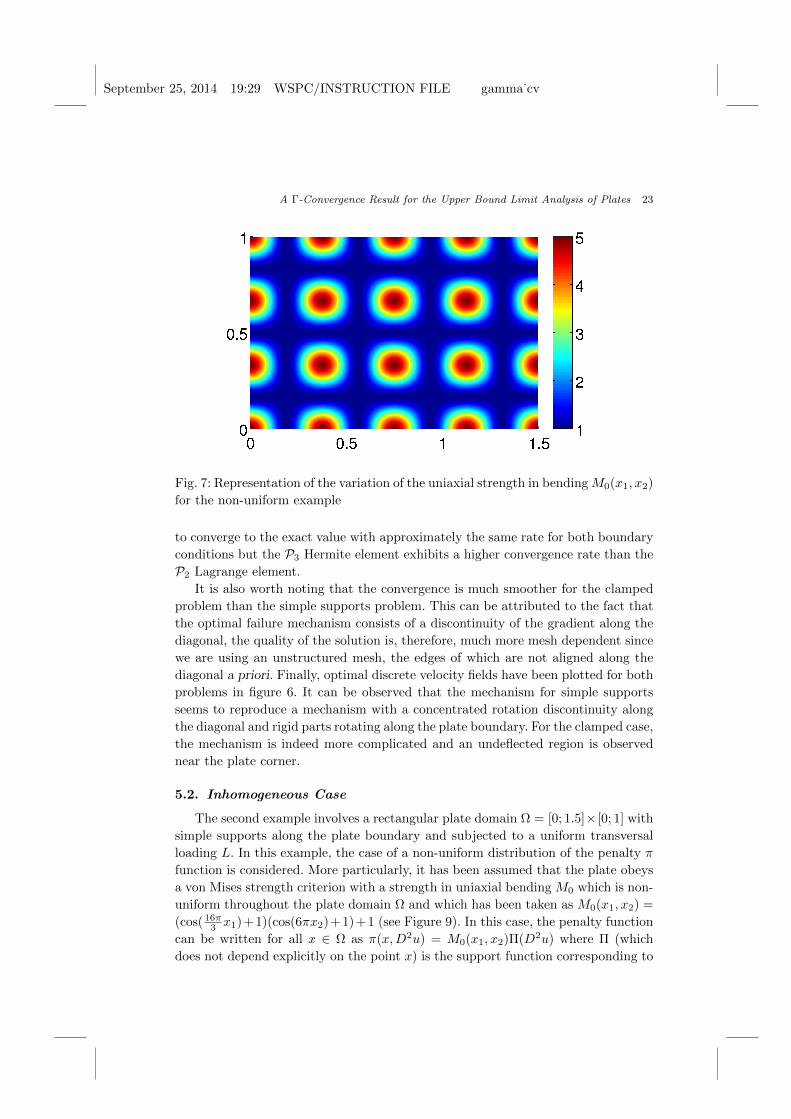
Fig. 7: Representation of the variation of the uniaxial strength in bendingM0(x1, x2)

for the non-uniform example

to converge to the exact value with approximately the same rate for both boundary

conditions but the P3 Hermite element exhibits a higher convergence rate than the

P2 Lagrange element.

It is also worth noting that the convergence is much smoother for the clamped

problem than the simple supports problem. This can be attributed to the fact that

the optimal failure mechanism consists of a discontinuity of the gradient along the

diagonal, the quality of the solution is, therefore, much more mesh dependent since

we are using an unstructured mesh, the edges of which are not aligned along the

diagonal a priori. Finally, optimal discrete velocity fields have been plotted for both

problems in figure 6. It can be observed that the mechanism for simple supports

seems to reproduce a mechanism with a concentrated rotation discontinuity along

the diagonal and rigid parts rotating along the plate boundary. For the clamped case,

the mechanism is indeed more complicated and an undeflected region is observed

near the plate corner.

5.2. Inhomogeneous Case

The second example involves a rectangular plate domain Ω = [0; 1.5]× [0; 1] with

simple supports along the plate boundary and subjected to a uniform transversal

loading L. In this example, the case of a non-uniform distribution of the penalty π

function is considered. More particularly, it has been assumed that the plate obeys

a von Mises strength criterion with a strength in uniaxial bending M0 which is non-

uniform throughout the plate domain Ω and which has been taken as M0(x1, x2) =

(cos( 16π3 x1)+1)(cos(6πx2)+1)+1 (see Figure 9). In this case, the penalty function

can be written for all x ∈ Ω as π(x,D2u) = M0(x1, x2)Π(D2u) where Π (which

does not depend explicitly on the point x) is the support function corresponding to



(a) Uniform distribution of M0

(b) Non-uniform distribution of M0

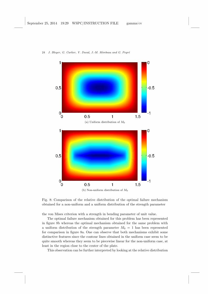
Fig. 8: Comparison of the relative distribution of the optimal failure mechanism

obtained for a non-uniform and a uniform distribution of the strength parameter

the von Mises criterion with a strength in bending parameter of unit value.

The optimal failure mechanism obtained for this problem has been represented

in figure 8b whereas the optimal mechanism obtained for the same problem with

a uniform distribution of the strength parameter M0 = 1 has been represented

for comparison in figure 8a. One can observe that both mechanisms exhibit some

distinctive features since the contour lines obtained in the uniform case seem to be

quite smooth whereas they seem to be piecewise linear for the non-uniform case, at

least in the region close to the center of the plate.

This observation can be further interpreted by looking at the relative distribution



(a) Uniform distribution of M0

(b) Non-uniform distribution of M0

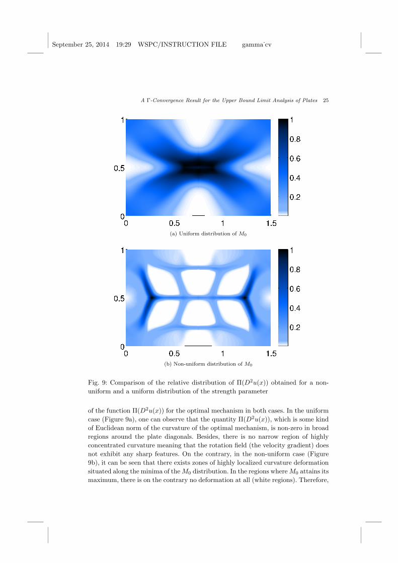
Fig. 9: Comparison of the relative distribution of Π(D2u(x)) obtained for a non-

uniform and a uniform distribution of the strength parameter

of the function Π(D2u(x)) for the optimal mechanism in both cases. In the uniform

case (Figure 9a), one can observe that the quantity Π(D2u(x)), which is some kind

of Euclidean norm of the curvature of the optimal mechanism, is non-zero in broad

regions around the plate diagonals. Besides, there is no narrow region of highly

concentrated curvature meaning that the rotation field (the velocity gradient) does

not exhibit any sharp features. On the contrary, in the non-uniform case (Figure

9b), it can be seen that there exists zones of highly localized curvature deformation

situated along the minima of theM0 distribution. In the regions whereM0 attains its

maximum, there is on the contrary no deformation at all (white regions). Therefore,


26 REFERENCES

in these regions, the optimal field is linear and there is a discontinuity of the rotation

field where M0 is minimal. This is valid essentially at the center of the plate since

it is not possible to obtain a piecewise linear velocity field along the minima around

the corners due to the boundary conditions.

Conclusion

In this article, we have provided for the first time a rigorous analysis of the con-

vergence of second order finite element discretizations for the limit analysis of thin

plates. This requires a careful definition of the corresponding continuous problem

over the space of Bounded Hessian functions. Handling second order derivatives

which are measures requires some special approximation arguments to ensure the

convergence of the finite element method.

Let us emphasize that, although we have insisted on the Lagrange and Hermite

finite elements, the proposed result holds in the more general case of any finite

element system which is affine equivalent (see [BS08]) to some reference element an

which involves derivatives up to the second order. Future works may extend this

approach to finer models such as the study of thick plates in bending and shear

forces.

Acknowledgements

The work of Gabriel Peyre and Vincent Duval has been supported by the Eu-

ropean Research Council (ERC project SIGMA-Vision).

References

Ada75. R. A. Adams. Sobolev spaces / Robert A. Adams. Academic Press New

York, 1975.

AFP00. L. Ambrosio, N. Fusco, and D. Pallara. Functions of Bounded Variation

and Free Discontinuity Problems. Oxford mathematical monographs.

Oxford University Press, 2000.

BdB13. J. Bleyer and P. de Buhan. On the performance of non-conforming finite

elements for the upper bound limit analysis of plates. International

Journal for Numerical Methods in Engineering, 94(3):308–330, 2013.

BDH89. H. Ben Dhia and T. Hadhri. Existence result and discontinuous finite

element discretization for a plane stresses hencky problem. Math. Meth.

in the Appl. Sci., 11:169–184, 1989.

Bra02. A. Braides. Gamma-convergence for Beginners. Oxford University

Press, USA, 2002.

Bræ71. M.W. Bræstrup. Yield-line theory and limit analysis of plates and slabs.

Danmarks Tekniske Højskole, Afdelingen for Bærende Konstruktioner,

1971.

BS08. S.C. Brenner and R. Scott. The Mathematical Theory of Finite Element

Methods. Texts in Applied Mathematics. Springer, 2008.


REFERENCES 27

CC99. A. Capsoni and L. Corradi. Limit analysis of plates- a finite element for-

mulation. Structural Engineering and Mechanics, 8(4):325–341, 1999.

CD79. P. Ciarlet and P. Destuynder. Justification of the 2-dimensional linear

plate model. Journal de Mecanique, 18(2):315–344, 1979.

Dem83. F. Demengel. Problemes variationnels en plasticite parfaite des plaques.

Numerical Functional Analysis and Optimization, 6(1):73–119, 1983.

Dem84. F. Demengel. Fonctions a hessien borne. Annales de l’institut Fourier,

34(2):155–190, 1984.

Dem89. F. Demengel. Compactness theorems for spaces of functions with

bounded derivatives and applications to limit analysis problems in plas-

ticity. Archive for Rational Mechanics and Analysis, 105(2):123–161,

1989.

DM93. G. Dal Maso. An Introduction to Γ-convergence, volume 8 of Progress

in nonlinear differential equations and their applications. Birkhauser,

Boston, MA, 1993.

DT84. F. Demengel and R. Temam. Convex function of a measure and its

applications. Indiana Univ. Math. J, 33(5):673–709, 1984.

Fox74. E.N. Fox. Limit analysis for plates: the exact solution for a clamped

square plate of isotropic homogeneous material obeying the square yield

criterion and loaded by uniform pressure. Philosophical Transactions

of the Royal Society of London. Series A, Mathematical and Physical

Sciences, 277(1265):121–155, 1974.

Had85a. T. Hadhri. Fonction convexe d’une mesure. C.R. Acad. Sci. Paris,

301:687–690, 1985.

Had85b. T. Hadhri. Etude dans HB × BD d’un modele de plaques

elastoplastiques comportant une non-linearite geometrique. ESAIM:

Mathematical Modelling and Numerical Analysis, 19(2):235–283, 1985.

Had86. T. Hadhri. Presentation et analyse mathematique de quelques modeles

pour des structures elastoplastiques homogenes ou heterogenes. These

d’etat, Universite Pierre et Marie Cure, Paris, 1986.

Had88. T. Hadhri. Prise en compte d’une force lineique de frontiere

dans un modele de plaques de hencky comportant une non-linearite

geometrique. ESAIM: Mathematical Modelling and Numerical Analy-

sis - Modelisation Mathematique et Analyse Numerique, 22(3):457–468,

1988.

HJB68. P.G. Hodge Jr and T. Belytschko. Numerical methods for the limit

analysis of plates. Journal of Applied Mechanics, 35(4):796, 1968.

Jen96. A. Jennings. On the identification of yield-line collapse mechanisms.

Engineering structures, 18(4):332–337, 1996.

Joh94. D. Johnson. Mechanism determination by automated yield-line analy-

sis. Structural Engineer, 72(19):323–323, 1994.

LGA09. C.V. Le, M. Gilbert, and H. Askes. Limit analysis of plates using the

EFG method and second-order cone programming. International Jour-


28 REFERENCES

nal for Numerical Methods in Engineering, 78(13):1532–1552, 2009.

LNXND10. C.V. Le, H. Nguyen-Xuan, and H. Nguyen-Dang. Upper and lower

bound limit analysis of plates using FEM and second-order cone pro-

gramming. Computers & Structures, 88(1-2):65–73, 2010.

MDF78. J. Munro and A.M.A. Da Fonseca. Yield line method by finite elements

and linear programming. Structural Engineer, 56(2):37–44, 1978.

Mos08. Mosek. The Mosek optimization toolbox for MATLAB manual, 2008.

OP11. C. Ortner and D. Praetorius. On the convergence of adaptive non-

conforming finite element methods for a class of convex variational

problems. SIAM J. Numer. Anal., 49(1):346–367, February 2011.

Pra59. W. Prager. An Introduction to Plasticity. Addison-Wesley series in the

engineering sciences: Mechanics and thermodynamics. Addison-Wesley

Pub. Co., 1959.

Roc83. T. Rockafellar. Convex Analysis, volume 224 of Grundlehren der mathe-

matischen Wissenschaften. Princeton University Press, second edition,

1983.

SMdS97. M.A. Save, C.E. Massonnet, and G. de Saxce. Plastic limit analysis of

plates, shells, and disks, volume 43. North Holland, 1997.

Tel95. J. J. Telega. Epi-limit on HB and homogenization of heterogeneous

plastic plates. Nonlinear Anal., 25(5):499–529, September 1995.

Tem85. R. Temam. Mathematical problems in plasticity. Gauthier-Villars Paris,

1985.

ZLC12. S. Zhou, Y. Liu, and S. Chen. Upper bound limit analysis of plates

utilizing the C1 natural element method. Computational Mechanics,

50(5):543–561, 2012.

A -Convergence Result for the Upper Bound Limit Analysis of Platescarlier/gamma_cv.pdf · A...

Documents

Transcript of A -Convergence Result for the Upper Bound Limit Analysis of Platescarlier/gamma_cv.pdf · A...