A Bahadur Representation

of the Linear Support Vector Machine

Ja-Yong Koo jykoo@korea.ac.kr

Department of StatisticsKorea UniversitySeoul, 136-701, Korea

Yoonkyung Lee yklee@stat.osu.edu

Department of StatisticsThe Ohio State UniversityColumbus, OH 43210, USA

Yuwon Kim yuwonkim@naver.com

Data Mining TeamNHN Inc.Gyeonggi-do 463-847, Korea

Changyi Park park463@uos.ac.kr

Department of Statistics

University of Seoul

Jeonnong-dong 90, Dongdaemun-gu

Seoul, 130-743, Korea

Abstract

The support vector machine has been successful in a variety of applications. Also onthe theoretical front, statistical properties of the support vector machine have been stud-ied quite extensively with a particular attention to its Bayes risk consistency under someconditions. In this paper, we study somewhat basic statistical properties of the supportvector machine yet to be investigated, namely the asymptotic behavior of the coefficientsof the linear support vector machine. A Bahadur type representation of the coefficients isestablished under appropriate conditions, and their asymptotic normality and statisticalvariability are derived on the basis of the representation. These asymptotic results do notonly help further our understanding of the support vector machine, but also they can beuseful for related statistical inferences.

Keywords: Asymptotic Normality, Bahadur Representation, Classification, ConvexityLemma, Radon Transform

1. Introduction

The support vector machine (SVM) introduced by Cortes and Vapnik (1995) has beensuccessful in many applications due to its high classification accuracy and flexibility. Forreference, see Vapnik (1996), Scholkopf and Smola (2002), and Cristianini and Shawe-Taylor(2000). In parallel with a wide range of applications, statistical properties of the SVM havebeen studied by many researchers recently in addition to the statistical learning theory by

1

Vapnik (1996) that originally motivated the SVM. These include studies on the Bayes riskconsistency of the SVM (Lin, 2002; Zhang, 2004; Steinwart, 2005) and its rate of convergenceto the Bayes risk (Lin, 2000; Blanchard, Bousquet, and Massart, 2004; Scovel and Steinwart,2006; Bartlett, Jordan, and McAuliffe, 2006). While the existing theoretical analysis of theSVM largely concerns its asymptotic risk, there are some basic statistical properties of theSVM that seem to have eluded our attention. For example, to the best of our knowledge,large sample properties of the coefficients in the linear SVM have not been studied so faralthough the magnitude of each coefficient is often the determining factor of feature selectionfor the SVM in practice.

In this paper, we address this basic question of the statistical behavior of the linearSVM as a first step to the study of more general properties of the SVM. We mainly inves-tigate asymptotic properties of the coefficients of variables in the SVM solution for linearclassification. The investigation is done in the standard way that parametric methods arestudied in a finite dimensional setting, that is, the number of variables is assumed to befixed and the sample size grows to infinity. Additionally, in the asymptotics, the effectof regularization through maximization of the class margin is assumed to vanish at a cer-tain rate so that the solution is ultimately governed by the empirical risk. Due to theseassumptions, the asymptotic results become more pertinent to the classical parametric set-ting where the number of features is moderate compared to the sample size and the virtueof regularization is minute than to the situation with high dimensional inputs. Despite thedifference between the practical situation where the SVM methods are effectively used andthe setting theoretically posited in this paper, the asymptotic results shed a new light onthe SVM from a classical parametric point of view. In particular, we establish a Bahadurtype representation of the coefficients as in the studies of sample quantiles and estimatesof regression quantiles. See Bahadur (1966) and Chaudhuri (1991) for reference. It turnsout that the Bahadur type representation of the SVM coefficients depends on Radon trans-form of the second moments of the variables. This representation illuminates how the socalled margins of the optimal separating hyperplane and the underlying probability distri-bution within and around the margins determine the statistical behavior of the estimatedcoefficients. Asymptotic normality of the coefficients then follows immediately from therepresentation. The proximity of the hinge loss function that defines the SVM solution tothe absolute error loss and its convexity allow such asymptotic results akin to those for leastabsolute deviation regression estimators in Pollard (1991).

In addition to providing an insight into the asymptotic behavior of the SVM, we expectthat our results can be useful for related statistical inferences on the SVM, for instance,feature selection. For introduction to feature selection, see Guyon and Elisseeff (2003), andfor an extensive empirical study of feature selection using SVM-based criteria, see Ishakand Ghattas (2005). In particular, Guyon, Weston, Barnhill, and Vapnik (2002) proposeda recursive feature elimination procedure for the SVM with an application to gene selectionin microarray data analysis. Its selection or elimination criterion is based on the absolutevalue of a coefficient not its standardized value. The asymptotic variability of estimatedcoefficients that we provide can be used in deriving a new feature selection criterion whichtakes inherent statistical variability into account.

This paper is organized as follows. Section 2 contains the main results of a Bahadur typerepresentation of the linear SVM coefficients and their asymptotic normality under mild

2

conditions. An illustrative example is then provided in Section 3 followed by simulationstudies in Section 4. Proofs of technical lemmas and theorems are collected in Section 5,ensued by a discussion in Section 6.

2. Main Results

2.1 Preliminaries

Let (X,Y ) be a pair of random variables with X ∈ X ⊂ Rd and Y ∈ {1,−1}. The marginal

distribution of Y is given by P(Y = 1) = π+ and P(Y = −1) = π− with π+, π− > 0 andπ+ + π− = 1. Let f and g be the densities of X given Y = 1 and −1, respectively. Let{(Xi, Y i)}n

i=1 be a set of training data, independently drawn from the distribution of (X,Y ).Denote the input variables as x = (x1, . . . , xd)

⊤ and their coefficients as β+ = (β1, . . . , βd)⊤.

Let x = (x0, . . . , xd)⊤ = (1, x1, . . . , xd)

⊤ and β = (β0, β1, . . . , βd)⊤. We consider linear

classifications with hyperplanes defined by h(x;β) = β0 + x⊤β+ = x⊤β. Let ‖ · ‖ denotethe Euclidean norm of a vector. For separable cases, the SVM finds the hyperplane thatmaximizes the geometric margin, 2/‖β+‖2 subject to the constraints yih(xi;β) ≥ 1 fori = 1, . . . , n. For non-separable cases, a soft-margin SVM is introduced to minimize

Cn∑

i=1

ξi +1

2‖β+‖2

subject to the constraints ξi ≥ 1 − yih(xi;β) and ξi ≥ 0 for i = 1, . . . , n, where C > 0is a tuning parameter and {ξi}n

i=1 are called the slack variables. Equivalently, the SVMminimizes the unconstrained objective function

lλ,n(β) =1

n

n∑

i=1

[1 − yih(xi;β)

]+

+λ

2‖β+‖2 (1)

over β ∈ Rd+1, where [z]+ = max(z, 0) for z ∈ R and λ > 0 is a penalization parameter; see

Vapnik (1996) for details. Let the minimizer of (1) be denoted by βλ,n = arg minβ lλ,n(β).Note that C = (nλ)−1. Choice of λ depends on the data, and usually it is estimated viacross validation in practice. In this paper, we consider only nonseparable cases and assumethat λ → 0 as n → ∞. We note that separable cases require a different treatment forasymptotics because λ has to be nonzero in the limit for the uniqueness of the solution.

Before we proceed with a discussion of the asymptotics of the βλ,n, we introduce somenotation and definitions first. The population version of (1) without the penalty term isdefined as

L(β) = E

[1 − Y h(X;β)

]+

(2)

and its minimizer is denoted by β∗ = arg minβ L(β). Then the population version of theoptimal hyperplane defined by the SVM is

x⊤β∗ = 0. (3)

Sets are identified with their indicator functions. For example,

∫

Xxj{xj > 0}f(x)dx =

∫

{x∈X : xj>0}xjf(x)dx. Letting ψ(z) = {z ≥ 0} for z ∈ R, we define S(β) = (S(β)j) to be

3

the (d+ 1)-dimensional vector given by

S(β) = −E

(ψ(1 − Y h(X;β))Y X

)

and H(β) = (H(β)jk) to be the (d+ 1) × (d+ 1)-dimensional matrix given by

H(β) = E

(δ(1 − Y h(X;β))XX⊤

),

where δ denotes the Dirac delta function with δ(t) = ψ′(t) in distributional sense. Providedthat S(β) and H(β) are well-defined, S(β) and H(β) are considered as the gradient andHessian matrix of L(β), respectively. Formal proofs of these relationships are given inSection 5.1.

For explanation of H(β), we introduce a Radon transformation. For a function s on X ,define the Radon transform Rs of s for p ∈ R and ξ ∈ R

d as

(Rs)(p, ξ) =

∫

Xδ(p − ξ⊤x)s(x)dx.

Denote

sj(x) = xjs(x), sjk(x) = xjxks(x) for 0 ≤ j, k ≤ d.

Then, it can be seen that

H(β)jk = π+(Rfjk)(1 − β0, β+) + π−(Rgjk)(1 + β0,−β+). (4)

Equation (4) shows that the Hessian matrix H(β) depends on the Radon transforms of f , g,fj, gj , fjk and gjk. For Radon transform and its properties in general, see Natterer (1986),Deans (1993), or Ramm and Katsevich (1996).

For a continuous integrable function s, it can be easily proved that Rs is continuous. If fand g are continuous densities with finite second moments, then fjk and gjk are continuousand integrable. Hence H(β) is continuous in β when f and g are continuous and have finitesecond moments.

2.2 Asymptotics

Now we present the asymptotic results for βλ,n. We state regularity conditions for the as-ymptotics first. Some remarks on the conditions then follow for exposition and clarification.Throughout this paper, we use C1, C2, . . . to denote positive constants independent of n.

(A1) The densities f and g are continuous and have finite second moments.

(A2) There exists B(x0, δ0), a ball centered at x0 with radius δ0 > 0 such that f(x) > C1

and g(x) > C1 for every x ∈ B(x0, δ0).

(A3) For some 1 ≤ i∗ ≤ d,

∫

X{xi∗ ≥ G−

i∗}xi∗g(x)dx <

∫

X{xi∗ ≤ F+

i∗ }xi∗f(x)dx

4

or ∫

X{xi∗ ≤ G+

i∗}xi∗g(x)dx >

∫

X{xi∗ ≥ F−

i∗ }xi∗f(x)dx.

Here F+i∗ , G

+i∗ ∈ [−∞,∞] are upper bounds such that

∫

X{xi∗ ≤ F+

i∗ }f(x)dx =

min

(1,π−π+

)and

∫

X{xi∗ ≤ G+

i∗}g(x)dx = min

(1,π+

π−

). Similarly, lower bounds

F−i∗ and G−

i∗ are defined as

∫

X{xi∗ ≥ F−

i∗ }f(x)dx = min

(1,π−π+

)and

∫

X{xi∗ ≥

G−i∗}g(x)dx = min

(1,π+

π−

).

(A4) For an orthogonal transformation Aj∗ that maps β∗+/‖β∗+‖ to the j∗-th unit vector ej∗

for some 1 ≤ j∗ ≤ d, there exist rectangles

D+ = {x ∈M+ : li ≤ (Aj∗x)i ≤ vi with li < vi for i 6= j∗}

andD− = {x ∈M− : li ≤ (Aj∗x)i ≤ vi with li < vi for i 6= j∗}

such that f(x) ≥ C2 > 0 on D+, and g(x) ≥ C3 > 0 on D−, where M+ = {x ∈X | β∗0 + x⊤β∗+ = 1} and M− = {x ∈ X | β∗0 + x⊤β∗+ = −1}.

Remark 1

• (A1) ensures that H(β) is well-defined and continuous in β.

• When f and g are continuous, the condition that f(x0) > 0 and g(x0) > 0 for somex0 implies (A2).

• The technical condition in (A3) is a minimal requirement to guarantee that β∗+, thenormal vector of the theoretically optimal hyperplane is not zero. Roughly speaking,it says that for at least one input variable, the mean values of the class conditionaldistributions f and g have to be different in order to avoid the degenerate case ofβ∗+ = 0. Some restriction of the supports through F+

i∗ , G+i∗, F

−i∗ and G−

i∗ is necessaryin defining the mean values to adjust for potentially unequal class proportions. Whenπ+ = π−, F+

i∗ and G+i∗ can be taken to be +∞ and F−

i∗ and G−i∗ can be −∞. In this

case, (A3) simply states that the mean vectors for the two classes are different.

• (A4) is needed for the positive-definiteness of H(β) around β∗. The condition meansthat there exist two subsets of the classification margins, M+ and M− on which theclass densities f and g are bounded away from zero. For mathematical simplicity, therectangular subsets D+ and D− are defined as the mirror images of each other alongthe normal direction of the optimal hyperplane. This condition can be easily met whenthe supports of f and g are convex. Especially, if R

d is the support of f and g, it istrivially satisfied. (A4) requires that β∗+ 6= 0, which is implied by (A1) and (A3); seeLemma 4 for the proof. For the special case d = 1, M+ and M− consist of a point.D+ and D− are the same as M+ and M−, respectively, and hence (A4) means thatf and g are positive at those points in M+ and M−.

5

Under the regularity conditions, we obtain a Bahadur-type representation of βλ,n (The-

orem 1). The asymptotic normality of βλ,n follows immediately from the representation

(Theorem 2). Consequently, we have the asymptotic normality of h(x; βλ,n), the value ofthe SVM decision function at x (Corollary 3).

Theorem 1 Suppose that (A1)-(A4) are met. For λ = o(n−1/2), we have

√n(βλ,n − β∗) = − 1√

nH(β∗)−1

n∑

i=1

ψ(1 − Y ih(Xi;β∗))Y iXi + oP(1).

Theorem 2 Suppose (A1)-(A4) are satisfied. For λ = o(n−1/2),

√n(βλ,n − β∗) → N

(0,H(β∗)−1G(β∗)H(β∗)−1

)

in distribution, where

G(β) = E

(ψ(1 − Y h(X;β))XX⊤

).

Remark 2 Since βλ,n is a consistent estimator of β∗ as n → ∞, G(β∗) can be estimated

by its empirical version with β∗ replaced by βλ,n. To estimate H(β∗), one may consider thefollowing nonparametric estimate:

1

n

[n∑

i=1

pb

(1 − Y ih(Xi; βλ,n)

)Xi(Xi)⊤

],

where pb(t) ≡ p(t/b)/b, p(t) ≥ 0 and∫

Rp(t)dt = 1. Note that pb(·) → δ(·) as b → 0.

However, estimation of H(β∗) requires further investigation.

Corollary 3 Under the same conditions as in Theorem 2,

√n(h(x; βλ,n) − h(x;β∗)

)→ N

(0, x⊤H(β∗)−1G(β∗)H(β∗)−1x

)

in distribution.

Remark 3 Corollary 3 can be used to construct a confidence bound for h(x;β∗) based onan estimate h(x; βλ,n), in particular, to judge whether h(x;β∗) is close to zero or not givenx. This may be useful if one wants to abstain from prediction at a new input x if it is closeto the optimal classification boundary h(x;β∗) = 0.

3. An Illustrative Example

In this section, we illustrate the relation between the Bayes decision boundary and theoptimal hyperplane determined by (2) for two multivariate normal distributions in R

d.Assume that f and g are multivariate normal densities with different mean vectors µf andµg and a common covariance matrix Σ. Suppose that π+ = π− = 1/2.

6

We verify the assumptions (A1)-(A4) so that Theorem 2 is applicable. For normaldensities f and g, (A1) holds trivially, and (A2) is satisfied with

C1 = |2πΣ|−1/2 exp

(− sup

‖x‖≤δ0

{(x− µf )⊤Σ−1(x− µf ), (x− µg)

⊤Σ−1(x− µg)})

for δ0 > 0. Since µf 6= µg, there exists 1 ≤ i∗ ≤ d such that i∗-th elements of µf and µg aredifferent. By taking F+

i∗ = G+i∗ = +∞ and F−

i∗ = G−i∗ = −∞, we can show that one of the

inequalities in (A3) holds as mentioned in Remark 1. Since D+ and D− can be taken to bebounded sets of the form in (A4) in R

d−1, and the normal densities f and g are boundedaway from zero on such D+ and D−, (A4) is satisfied. In particular, β∗+ 6= 0 as implied byLemma 4.

Denote the density and cumulative distribution function of N(0, 1) as φ and Φ, respec-tively. Note that β∗ should satisfy the equation S(β∗) = 0, or

Φ(af ) = Φ(ag) (5)

andµfΦ(af ) − φ(af )Σ1/2ω∗ = µgΦ(ag) + φ(ag)Σ

1/2ω∗, (6)

where af =1 − β∗0 − µ⊤f β

∗+

‖Σ1/2β∗+‖, ag =

1 + β∗0 + µ⊤g β∗+

‖Σ1/2β∗+‖and ω∗ = Σ1/2β∗+/‖Σ1/2β∗+‖. From (5)

and the definition of af and ag, we have a∗ ≡ af = ag. Hence

(β∗+)⊤(µf + µg) = −2β∗0 . (7)

It follows from (6) that

β∗+/‖Σ1/2β∗+‖ =Φ(a∗)2φ(a∗)

Σ−1(µf − µg). (8)

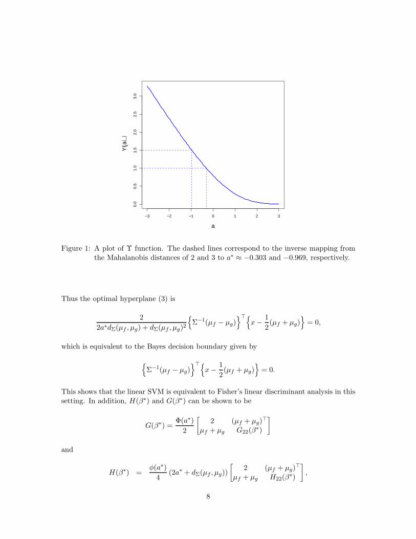
First we show the existence of a proper constant a∗ satisfying (8) and its relationship witha statistical distance between the two classes. Define Υ(a) = φ(a)/Φ(a) and let dΣ(u, v) ={(u − v)⊤Σ−1(u − v)}1/2 denote the Mahalanobis distance between u and v ∈ R

d. Since‖ω∗‖ = 1, we have Υ(a∗) = ‖Σ−1/2(µf − µg)‖/2. Since Υ(a) is monotonically decreasing ina, there exists a∗ = Υ−1(dΣ(µf , µg)/2) that depends only on µf , µg, and Σ. For illustration,when the Mahalanobis distances between the two normal distributions are 2 and 3, a∗ isgiven by Υ−1(1) ≈ −0.303 and Υ−1(1.5) ≈ −0.969, respectively. The corresponding Bayeserror rates are about 0.1587 and 0.06681. Figure 1 shows a graph of Υ(a) and a∗ whendΣ(µf , µg)=2 and 3.

Once a∗ is properly determined, we can express the solution β∗ explicitly by (7) and(8):

β∗0 = − (µf − µg)⊤Σ−1(µf + µg)

2a∗dΣ(µf , µg) + dΣ(µf , µg)2

and

β∗+ =2Σ−1(µf − µg)

2a∗dΣ(µf , µg) + dΣ(µf , µg)2.

7

−3 −2 −1 0 1 2 3

0.0

0.5

1.0

1.5

2.0

2.5

3.0

a

Υ(a

)

Figure 1: A plot of Υ function. The dashed lines correspond to the inverse mapping fromthe Mahalanobis distances of 2 and 3 to a∗ ≈ −0.303 and −0.969, respectively.

Thus the optimal hyperplane (3) is

2

2a∗dΣ(µf , µg) + dΣ(µf , µg)2

{Σ−1(µf − µg)

}⊤{x− 1

2(µf + µg)

}= 0,

which is equivalent to the Bayes decision boundary given by

{Σ−1(µf − µg)

}⊤{x− 1

2(µf + µg)

}= 0.

This shows that the linear SVM is equivalent to Fisher’s linear discriminant analysis in thissetting. In addition, H(β∗) and G(β∗) can be shown to be

G(β∗) =Φ(a∗)

2

[2 (µf + µg)

⊤

µf + µg G22(β∗)

]

and

H(β∗) =φ(a∗)

4(2a∗ + dΣ(µf , µg))

[2 (µf + µg)

⊤

µf + µg H22(β∗)

],

8

where

G22(β∗) = µfµ

⊤f + µgµ

⊤g + 2Σ −

(a∗

dΣ(µf , µg)+ 1

)(µf − µg)(µf − µg)

⊤ and

H22(β∗) = µfµ

⊤f + µgµ

⊤g + 2Σ

+2

((a∗

dΣ(µf , µg)

)2

+a∗

dΣ(µf , µg)− 1

d2Σ(µf , µg)

)(µf − µg)(µf − µg)

⊤.

0 1 2 3 4 5 6

010

2030

4050

Mahalanobis distance

asym

ptot

ic v

aria

bilit

y

(a)

0 1 2 3 4 5 6

010

2030

4050

Mahalanobis distance

asym

ptot

ic v

aria

bilit

y

(b)

0 1 2 3 4 5 6

010

2030

4050

Mahalanobis distance

asym

ptot

ic v

aria

bilit

y

(c)

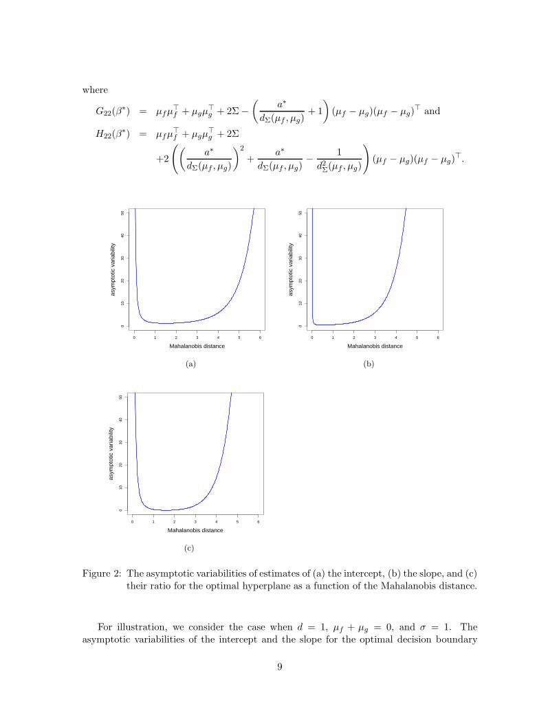
Figure 2: The asymptotic variabilities of estimates of (a) the intercept, (b) the slope, and (c)their ratio for the optimal hyperplane as a function of the Mahalanobis distance.

For illustration, we consider the case when d = 1, µf + µg = 0, and σ = 1. Theasymptotic variabilities of the intercept and the slope for the optimal decision boundary

9

are calculated according to Theorem 2. Figure 2 shows the asymptotic variabilities as afunction of the Mahalanobis distance between the two normal distributions, |µf −µg| in thiscase. Also, it depicts the asymptotic variance of the estimated classification boundary value(−β0/β1) by using the delta method. Although the Mahalanobis distance roughly in therange of 1 to 4 would be of practical interest, the plots show a notable trend in the asymptoticvariances as the distance varies. When the two classes get very close, the variances shootup due to the difficulty in discriminating them. On the other hand, as the Mahalanobisdistance increases, that is, the two classes become more separated, the variances becomeincreasingly large. A possible explanation for the trend is that the intercept and the slopeof the optimal hyperplane are determined by only a small fraction of data falling into themargins in this case.

4. Simulation Studies

In this section, simulations are carried out to illustrate the asymptotic results and theirpotential for feature selection.

4.1 Bivariate Case

Theorem 2 is numerically illustrated with the multivariate normal setting in the previoussection. Consider a bivariate case with mean vectors µf = (1, 1)⊤ and µg = (−1,−1)⊤

and a common covariance matrix Σ = I2. This example has dΣ(µf , µg) = 2√

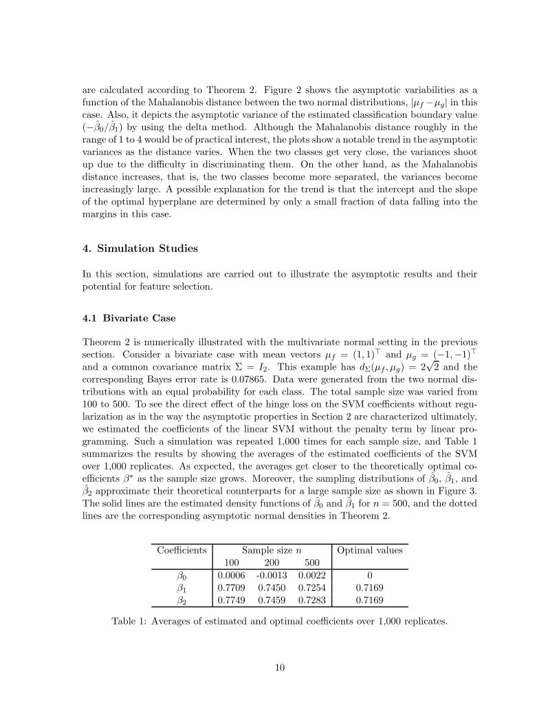
2 and thecorresponding Bayes error rate is 0.07865. Data were generated from the two normal dis-tributions with an equal probability for each class. The total sample size was varied from100 to 500. To see the direct effect of the hinge loss on the SVM coefficients without regu-larization as in the way the asymptotic properties in Section 2 are characterized ultimately,we estimated the coefficients of the linear SVM without the penalty term by linear pro-gramming. Such a simulation was repeated 1,000 times for each sample size, and Table 1summarizes the results by showing the averages of the estimated coefficients of the SVMover 1,000 replicates. As expected, the averages get closer to the theoretically optimal co-efficients β∗ as the sample size grows. Moreover, the sampling distributions of β0, β1, andβ2 approximate their theoretical counterparts for a large sample size as shown in Figure 3.The solid lines are the estimated density functions of β0 and β1 for n = 500, and the dottedlines are the corresponding asymptotic normal densities in Theorem 2.

Coefficients Sample size n Optimal values100 200 500

β0 0.0006 -0.0013 0.0022 0β1 0.7709 0.7450 0.7254 0.7169β2 0.7749 0.7459 0.7283 0.7169

Table 1: Averages of estimated and optimal coefficients over 1,000 replicates.

10

−0.4 −0.2 0.0 0.2 0.4

01

23

Den

sity

estimateasymptotic

(a)

0.5 0.6 0.7 0.8 0.9 1.0

01

23

45

Den

sity

estimateasymptotic

(b)

Figure 3: Estimated sampling distributions of (a) β0 and (b) β1 with the asymptotic normaldensities overlaid.

4.2 Feature Selection

Clearly the results we have established have implications to statistical inferences on theSVM. Among others, feature selection is of particular interest. By using the asymptoticvariability of estimated coefficients, one can derive a new feature selection criterion basedon the standardized coefficients. Such a criterion will take inherent statistical variabilityinto account. More generally, this consideration of new criteria opens the possibility ofcasting feature selection for the SVM formally in the framework of hypothesis testing andextending standard variable selection procedures in regression to classification.

We investigate the possibility of using the standardized coefficients of β for selection ofvariables. For practical applications, one needs to construct a reasonable nonparametricestimator of the asymptotic variance-covariance matrix, whose entries are defined throughline integrals. A similar technical issue arises in quantile regression. See Koenker (2005) forsome suggested variance estimators in the setting.

For the sake of simplicity in the second set of simulation, we used the theoretical asymp-totic variance in standardizing β and selected those variables with the absolute standardizedcoefficient exceeding a certain critical value. And we mainly monitored the type I error rateof falsely declaring the significance of a variable when it is not, over various settings of amixture of two multivariate normal distributions. Different combinations of the sample size(n) and the number of variables (d) were tried. For a fixed even d, we set µf = (1d/2,0d/2)

⊤,

µg = 0⊤d , and Σ = Id, where 1p and 0p indicate p-vectors of ones and zeros, respectively.

Thus only the first half of the d variables have nonzero coefficients in the optimal hyper-plane of the linear SVM. Table 2 shows the minima, median, and maxima of such type Ierror rates in selection of relevant variables over 200 replicates when the critical value wasz0.025 ≈ 1.96 (5% level of significance). If the asymptotic distributions were accurate, the

11

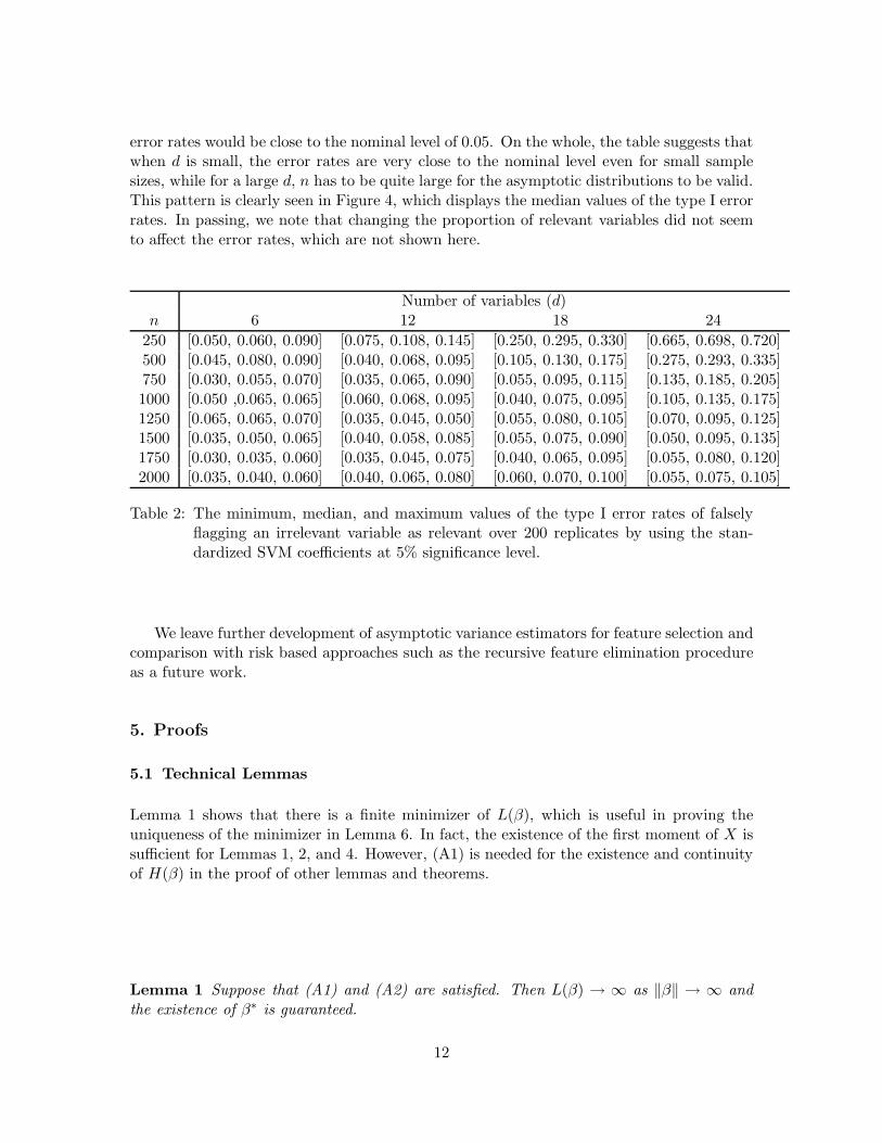
error rates would be close to the nominal level of 0.05. On the whole, the table suggests thatwhen d is small, the error rates are very close to the nominal level even for small samplesizes, while for a large d, n has to be quite large for the asymptotic distributions to be valid.This pattern is clearly seen in Figure 4, which displays the median values of the type I errorrates. In passing, we note that changing the proportion of relevant variables did not seemto affect the error rates, which are not shown here.

Number of variables (d)n 6 12 18 24

250 [0.050, 0.060, 0.090] [0.075, 0.108, 0.145] [0.250, 0.295, 0.330] [0.665, 0.698, 0.720]500 [0.045, 0.080, 0.090] [0.040, 0.068, 0.095] [0.105, 0.130, 0.175] [0.275, 0.293, 0.335]750 [0.030, 0.055, 0.070] [0.035, 0.065, 0.090] [0.055, 0.095, 0.115] [0.135, 0.185, 0.205]1000 [0.050 ,0.065, 0.065] [0.060, 0.068, 0.095] [0.040, 0.075, 0.095] [0.105, 0.135, 0.175]1250 [0.065, 0.065, 0.070] [0.035, 0.045, 0.050] [0.055, 0.080, 0.105] [0.070, 0.095, 0.125]1500 [0.035, 0.050, 0.065] [0.040, 0.058, 0.085] [0.055, 0.075, 0.090] [0.050, 0.095, 0.135]1750 [0.030, 0.035, 0.060] [0.035, 0.045, 0.075] [0.040, 0.065, 0.095] [0.055, 0.080, 0.120]2000 [0.035, 0.040, 0.060] [0.040, 0.065, 0.080] [0.060, 0.070, 0.100] [0.055, 0.075, 0.105]

Table 2: The minimum, median, and maximum values of the type I error rates of falselyflagging an irrelevant variable as relevant over 200 replicates by using the stan-dardized SVM coefficients at 5% significance level.

We leave further development of asymptotic variance estimators for feature selection andcomparison with risk based approaches such as the recursive feature elimination procedureas a future work.

5. Proofs

5.1 Technical Lemmas

Lemma 1 shows that there is a finite minimizer of L(β), which is useful in proving theuniqueness of the minimizer in Lemma 6. In fact, the existence of the first moment of X issufficient for Lemmas 1, 2, and 4. However, (A1) is needed for the existence and continuityof H(β) in the proof of other lemmas and theorems.

Lemma 1 Suppose that (A1) and (A2) are satisfied. Then L(β) → ∞ as ‖β‖ → ∞ andthe existence of β∗ is guaranteed.

12

500 1000 1500 2000

0.0

0.1

0.2

0.3

0.4

0.5

0.6

0.7

n

Typ

e I e

rror

rat

e

d=6d=12d=18d=24

Figure 4: The median values of the type I error rates in variable selection depending onthe sample size n and the number of variables d. The dotted line indicates thenominal level of 0.05.

Proof. Without loss of generality, we may assume that x0 = 0 in (A2) and B(0, δ0) ⊂ X .For any ε > 0,

L(β) = π+

∫

X[1 − x⊤β]+f(x)dx+ π−

∫

X[1 + h(x;β)]+g(x)dx

≥ π+

∫

X{h(x;β) ≤ 0}(1 − h(x;β))f(x)dx + π−

∫

X{h(x;β) ≥ 0}(1 + h(x;β))g(x)dx

≥ π+

∫

X{h(x;β) ≤ 0}(−h(x;β))f(x)dx + π−

∫

X{h(x;β) ≥ 0}h(x;β)g(x)dx

≥∫

X|h(x;β)|min (π+f(x), π−g(x)) dx

≥ C1 min(π+, π−)

∫

B(0,δ0)|h(x;β)|dx

= C1 min(π+, π−)‖β‖∫

B(0,δ0)|h(x;w)|dx

≥ C1 min(π+, π−)‖β‖vol ({|h(x;w)| ≥ ε} ∩B(0, δ0)) ε,

where w = β/‖β‖ and vol(A) denotes the volume of a set A.

13

Note that −1 ≤ w0 ≤ 1. For 0 ≤ w0 < 1 and 0 < ε < 1,

vol ({|h(x;w)| ≥ ε} ∩B(0, δ0))

≥ vol ({h(x;w) ≥ ε} ∩B(0, δ0))

= vol

({x⊤w+/

√1 − w2

0 ≥ (ε− w0)/√

1 −w20

}∩B(0, δ0)

)

≥ vol

({x⊤w+/

√1 − w2

0 ≥ ε

}∩B(0, δ0)

)≡ V (δ0, ε)

since (ε− w0)/√

1 − w20 ≤ ε. When −1 < w0 < 0, we obtain

volB(h(x;w) ≤ −ε) ≥ V (δ0, ε)

in a similar way. Note that V (δ0, ε) is independent of β and V (δ0, ε) > 0 for some ε < δ0.Consequently, L(β) ≥ C1 min(π+, π−)‖β‖V (δ0, ε)ε → ∞ as ‖β‖ → ∞. The case w0 = ±1is trivial.

Since the hinge loss is convex, L(β) is convex in β. Since L(β) → ∞ as ‖β‖ → ∞, theset, denoted by M, of minimizers of L(β) forms a bounded connected set. The existence ofthe solution β∗ of L(β) easily follows from this. �

In Lemmas 2 and 3, we obtain explicit forms of S(β) and H(β) for non-constant decisionfunctions.

Lemma 2 Assume that (A1) is satisfied. If β+ 6= 0, then we have

∂L(β)

∂βj= S(β)j

for 0 ≤ j ≤ d.

Proof. It suffices to show that

∂

∂βj

∫

X[1 − h(x;β)]+f(x)dx = −

∫

X{h(x;β) ≤ 1}xjf(x)dx.

Define ∆(t) = [1 − h(x;β) − txj]+ − [1 − h(x;β)]+. Let t > 0.

First, consider the case xj > 0. Then,

∆(t) =

0 if h(x;β) > 1h(x;β) − 1 if 1 − txj < h(x;β) ≤ 1−txj if h(x;β) ≤ 1 − txj.

Observe that∫

X∆(t){xj > 0}f(x)dx =

∫

X{1 − txj < h(x;β) ≤ 1}(h(x;β) − 1)f(x)dx

−t∫

X{h(x;β) ≤ 1 − txj, xj > 0}xjf(x)dx

14

and that∣∣∣∣1

t

∫

X{1 − txj < h(x;β) ≤ 1}(h(x;β) − 1)f(x)dx

∣∣∣∣ ≤∫

X{1 − txj < h(x;β) ≤ 1}xjf(x)dx.

By Dominated Convergence Theorem,

limt↓0

∫

X{1 − txj < h(x;β) ≤ 1}xjf(x)dx =

∫

X{h(x;β) = 1}xjf(x)dx = 0

and

limt↓0

∫

X{h(x;β) ≤ 1 − txj, xj > 0}xjf(x)dx =

∫

X{h(x;β) ≤ 1, xj > 0}xjf(x)dx.

Hence

limt↓0

1

t

∫

X∆(t){xj > 0}f(x)dx = −

∫

X{h(x;β) ≤ 1, xj > 0}xjf(x)dx. (9)

Now assume that xj < 0. Then,

∆(t) =

0 if h(x;β) > 1 − txj

1 − h(x;β) − txj if 1 < h(x;β) ≤ 1 − txj

−txj if h(x;β) ≤ 1.

In a similar fashion, one can show that

limt↓0

1

t

∫

X∆(t){xj < 0}f(x)dx = −

∫

X{h(x;β) ≤ 1, xj < 0}xjf(x)dx. (10)

Combining (9) and (10), we have shown that

limt↓0

1

t

∫

X∆(t)f(x)dx = −

∫

X{h(x;β) ≤ 1}xjf(x)dx.

The proof for the case t < 0 is similar. �

The proof of Lemma 3 is based on the following identity

∫δ(Dt+ E)T (t)dt =

1

|D|T (−E/D) (11)

for constants D and E. This identity follows from the fact that δ(at) = δ(t)/|a| and∫δ(t− a)T (t)dt = T (a) for a constant a.

Lemma 3 Suppose that (A1) is satisfied. Under the condition that β+ 6= 0, we have

∂2L(β)

∂βj∂βk= H(β)jk,

for 0 ≤ j, k ≤ d.

15

Proof. Define

Ψ(β) =

∫

X{x⊤β+ < 1 − β0}s(x)dx

for a continuous and integrable function s defined on X . Without loss of generality, we mayassume that β1 6= 0. It is sufficient to show that for 0 ≤ j, k ≤ d,

∂2

∂βj∂βk

∫

X[1 − h(x;β)]+f(x)dx =

∫

Xδ(1 − h(x;β))xj xkf(x)dx.

Define X−j = {(x1, . . . , xj−1, xj+1, . . . , xd) : (x1, . . . , xd) ∈ X} and Xj = {xj :(x1, . . . , xd) ∈ X}. Observe that

∂Ψ(β)

∂β0= − 1

|β1|

∫

X−1

s

(1 − h(x;β) + β1x1

β1, x2, . . . , xd

)dx−1 (12)

and that for k 6= 1,

∂Ψ(β)

∂βk= − 1

|β1|

∫

X−1

xks

(1 − h(x;β) + β1x1

β1, x2, . . . , xd

)dx−1. (13)

If βp = 0 for any p 6= 1, then

∂Ψ(β)

∂β1= −1 − β0

β1|β1|

∫

X−1

s

(1 − β0

β1, x2, . . . , xd

)dx−1. (14)

If there is p 6= 1 with βp 6= 0, then we have

∂Ψ(β)

∂β1= − 1

|βp|

∫

X−p

x1s

(x1, . . . , xp−1,

1 − h(x;β) + βpxp

βp, xp+1, . . . , xd

)dx−p. (15)

Choose D = β1, E = x⊤β − β1x1 − 1, t = x1 in (11). It follows from (13) and (15) that

∂Ψ(β)

∂βk= − 1

|β1|

∫

X−1

xks

(1 − h(x;β) + β1x1

β1, x2, . . . , xd

)dx−1 (16)

= −∫

X−1

∫

X1

xks(x)δ(h(x;β) − 1)dx1dx−1

= −∫

Xδ(1 − h(x;β))xks(x)dx.

Similarly, we have∂Ψ(β)

∂β0= −

∫

Xδ(1 − h(x;β))s(x)dx (17)

by (12).Choosing D = β1, E = β0 − 1, t = x1 in (11), we have

∫

X1

δ(β1x1 − 1 + β0)x1s(x)dx1 =1

|β1|

(1 − β0

β1

)s

(1 − β0

β1, x2, . . . , xd

)

by (14). This implies (16) for k = 1. The desired result now follows from (16) and (17). �

The following lemma asserts that the optimal decision function is not a constant underthe condition that the centers of two classes are separated.

16

Lemma 4 Suppose that (A1) is satisfied. Then (A3) implies that β∗+ 6= 0.

Proof. Suppose that∫

X{xi∗ ≥ G−

i∗}xi∗g(x)dx <

∫

X{xi∗ ≤ F+

i∗ }xi∗f(x)dx (18)

in (A3). We will show that

minβ0

L(β0, 0, . . . 0) > minβ0,βi∗>0

L(β0, 0, . . . , 0, βi∗ , 0, . . . , 0), (19)

implying that β∗+ 6= 0. Henceforth, we will suppress β’s that are equal to zero in L(β). Thepopulation minimizer (β∗0 , β

∗i∗) is given by the minimizer of

L(β0, βi∗) = π+

∫

X[1 − β0 − βi∗xi∗ ]+f(x)dx+ π−

∫

X[1 + β0 + βi∗xi∗ ]+g(x)dx.

First, consider the case βi∗ = 0.

L(β0) =

π−(1 + β0), β0 > 11 + (π− − π+)β0, −1 ≤ β0 ≤ 1π+(1 − β0), β0 < −1

with its minimumminβ0

L(β0) = 2min (π+, π−) . (20)

Now consider the case βi∗ > 0, where

L(β0, βi∗) = π+

∫

X

{xi∗ ≤ 1 − β0

βi∗

}(1 − β0 − βi∗xi∗)f(x)dx

+π−

∫

X

{xi∗ ≥ −1 − β0

βi∗

}(1 + β0 + βi∗xi∗)g(x)dx.

Let β0 denote the minimizer of L(β0, βi∗) for a given βi∗ . Note that ∂L(β0, βi∗)/∂β0 is givenas

∂L(β0, βi∗)

∂β0(21)

= −π+

∫

X

{xi∗ ≤ 1 − β0

βi∗

}f(x)dx+ π−

∫

X

{xi∗ ≥ −1 − β0

βi∗

}g(x)dx,

which is monotonic increasing in β0 with limβ0→−∞∂L(β0,βi∗)

∂β0→ −π+ and limβ0→∞

∂L(β0,βi∗)∂β0

→ π−. Hence β0 exists for a given βi∗ .When π− < π+, we can easily check that F+

i∗ <∞ and G−i∗ = −∞. F+

i∗ and G−i∗ may not

be determined uniquely, meaning that there may exist an interval with probability zero.There is no significant change in the proof under the assumption that F+

i∗ and G−i∗ are

unique. Note that

1 − β0

βi∗≤ F+

i∗

17

by definition of F+i∗ and (21). Then,

−1 − β0

βi∗≤ F+

i∗ − 2

βi∗→ −∞ as βi∗ → 0,

and1 − β0

βi∗→ F+

i∗ as βi∗ → 0.

¿From (18),

π−

∫

Xxi∗g(x)dx < π+

∫

X{xi∗ ≤ F+

i∗ }xi∗f(x)dx. (22)

Now consider the minimum of L(β0, βi∗) with respect to βi∗ > 0. From (21),

L(β0, βi∗) (23)

= π+

∫

X

{xi∗ ≤ 1 − β0

βi∗

}(1 − β0 − βi∗xi∗)f(x)dx

+π−

∫

X

{xi∗ ≥ −1 − β0

βi∗

}(1 + β0 + βi∗xi∗)g(x)dx

= 2π−

∫

X

{xi∗ ≥ −1 − β0

βi∗

}g(x)dx

+βi∗

(π−

∫

X

{xi∗ ≥ −1 − β0

βi∗

}xi∗g(x)dx − π+

∫

X

{xi∗ ≤ 1 − β0

βi∗

}xi∗f(x)dx

)

By (22), it can be easily seen that the second term in (23) is negative for sufficiently smallβi∗ > 0, implying

L(β0, βi∗) < 2π− for some βi∗ > 0.

If π− > π+, then F+i∗ = ∞ and G−

i∗ > −∞. Similarly, it can be checked that

L(β0, βi∗) < 2π+ for some βi∗ > 0.

Suppose that π− = π+. Then it can be verified that

1 − β0

βi∗→ ∞ as βi∗ → 0,

and−1 − β0

βi∗→ −∞ as βi∗ → 0.

In this case, L(β0, βi∗) < 1.

Hence, under (18), we have shown that

L(β0, βi∗) < 1 for some βi∗ > 0.

18

This, together with (20), implies (19). For the second case in (A3), the same argumentshold with βi∗ < 0. �

Note that (A1) implies that H is well-defined and continuous in its argument. (A4)ensures that H(β) is positive definite around β∗ and thus we have a lower bound result inLemma 5.

Lemma 5 Under (A1), (A3) and (A4),

β⊤H(β∗)β ≥ C4‖β‖2,

where C4 may depend on β∗.

Proof. Since the proof for the case d = 1 is trivial, we consider the case d ≥ 2 only. Observethat

β⊤H(β∗)β = E

(δ(1 − Y h(X;β∗))h2(X;β)

)

= π+

∫

Xδ(1 − h(x;β∗))h2(x;β)f(x)dx + π−

∫

Xδ(1 + h(x;β∗))h2(x;β)g(x)dx

= π+(Rh2f)(1 − β∗0 , β∗+) + π−(Rh2g)(1 + β∗0 ,−β∗+)

= π+(Rh2f)(1 − β∗0 , β∗+) + π−(Rh2g)(−1 − β∗0 , β

∗+).

The last equality follows from the homogeneity of Radon transform.

Recall that β∗+ 6= 0 by Lemma 4. Without loss of generality, we assume that j∗ = 1in (A4). Let A1β+ = a = (a1, . . . , ad) and z = (A1x)/‖β∗+‖. Given u = (u2, . . . , ud), let

u∗ =((1 − β∗0)/‖β∗+‖, u

). Define Z = {z = (A1x)/‖β∗+‖ : x ∈ X} and U = {u : uj =

‖β∗+‖zj for j = 2, . . . , d, and z ∈ Z}. Note that detA1 = 1, du = ‖β∗+‖d−1dz2 . . . dzd,

‖β∗+‖A⊤1 z∣∣∣z1=(1−β∗

0)/‖β∗

+‖2

= A⊤1

(1 − β∗0)/‖β∗+‖‖β∗+‖z2

...‖β∗+‖zd

= A⊤

1 u∗

and

β0 + ‖β∗+‖a⊤z∣∣∣z1=(1−β∗

0)/‖β∗

+‖2

= β0 + ‖β∗+‖(a1(1 − β∗0)/‖β∗+‖2 +

d∑

j=2

ajzj

)

= β0 + a1(1 − β∗0)/‖β∗+‖ + ‖β∗+‖d∑

j=2

ajzj.

19

Using the transformation A1, we have

(Rh2f)(1 − β∗0 , β∗+)

=

∫

Zδ(1 − β∗0 − ‖β∗+‖(A1β

∗+)⊤z

)h2(‖β∗+‖A⊤

1 z;β)f(‖β∗+‖A⊤

1 z)‖β∗+‖ddz

=

∫

Zδ(1 − β∗0 − ‖β∗+‖2e⊤1 z

)(β0 + ‖β∗+‖(A1β+)⊤z

)2f(‖β∗+‖A⊤

1 z)‖β∗+‖ddz

=

∫

Zδ(1 − β∗0 − ‖β∗+‖2z1

)(β0 + ‖β∗+‖a⊤z

)2f(‖β∗+‖A⊤

1 z)‖β∗+‖ddz

=1

‖β∗+‖

∫

U

(β0 + a1(1 − β∗0)/‖β∗+‖ +

d∑

j=2

ajuj

)2f(A⊤

1 u∗)du.

The last equality follows from the identity (11). Let D+∗ =

{u : A⊤

1 u∗ ∈ D+

}. By (A4),

there exists a constant C2 > 0 and a rectangle D+∗ on which f(A⊤

1 u∗) ≥ C2 for u ∈ D+

∗ .Then

(Rh2f)(1 − β∗0 , β∗+)

≥ 1

‖β∗+‖

∫

D+∗

(β0 + a1(1 − β∗0)/‖β∗+‖ +

d∑

j=2

ajuj

)2f(A⊤

1 u∗)du

≥ 1

‖β∗+‖· C2

∫

D+∗

(β0 + a1(1 − β∗0)/‖β∗+‖ +

d∑

j=2

ajuj

)2du

=1

‖β∗+‖· C2 · vol(D+

∗ )Eu(β0 + a1(1 − β∗0)/‖β∗+‖ +

d∑

j=2

ajUj

)2

=1

‖β∗+‖· C2 · vol(D+

∗ ){(β0 + a1(1 − β∗0)/‖β∗+‖ + E

ud∑

j=2

ajUj

)2+ V

u(d∑

j=2

ajUj)},

where Uj for j = 2, . . . , d are independent and uniform random variables defined on D+∗ , and

Eu and V

u denote the expectation and variance with respect to the uniform distribution.Letting µi = (li + vi)/2, we have

(Rh2f)(1 − β∗0 , β∗+) (24)

≥ 1

‖β∗+‖· C2 · vol(D+

∗ ){(β0 + a1(1 − β∗0)/‖β∗+‖ +

d∑

j=2

ajµj

)2+ min

2≤j≤dV

u(Uj)

d∑

j=2

a2j

}.

Similarly, it can be shown that

(Rh2g)(−1 − β∗0 , β∗+) (25)

≥ 1

‖β∗+‖· C3 · vol(D−

∗ ){(β0 − a1(1 + β∗0)/‖β∗+‖ +

d∑

j=2

ajµj

)2+ min

2≤j≤dV

u(Uj)d∑

j=2

a2j

},

where D−∗ =

{u : A⊤

1

((−1 − β∗0)/‖β∗+‖, u

)∈ D−

}.

20

Combining (24)-(25) and letting C5 = 2/‖β∗+‖min(π+C2 ·vol(D+

∗ ), π−C3 ·vol(D−∗ ))

and

C6 = min(1,min2≤j≤d V

u(Uj)), we have

β⊤H(β∗)β

≥ π+

‖β∗+‖· C2 · vol(D+

∗ ){(β0 + a1(1 − β∗0)/‖β∗+‖ +

d∑

j=2

aj µj

)2+ min

2≤j≤dV

u(Uj)

d∑

j=2

a2j

}

+π−‖β∗+‖

· C3 · vol(D−∗ ){(β0 − a1(1 + β∗0)/‖β∗+‖ +

d∑

j=2

ajµj

)2+ min

2≤j≤dV

u(Uj)d∑

j=2

a2j

}

≥ C5C6

{(β0 + a1(1 − β∗0)/‖β∗+‖ +

d∑

j=2

aj µj

)2

+(β0 − a1(1 + β∗0)/‖β∗+‖ +

d∑

j=2

ajµj

)2+ 2

d∑

j=2

a2j

}/2

= C5C6

{(β0 + a1(1 − β∗0)/‖β∗+‖

)2+(β0 − a1(1 + β∗0)/‖β∗+‖

)2

+4(β0 − a1β

∗0/‖β∗+‖

) d∑

j=2

aj µj + 2( d∑

j=2

aj µj

)2+ 2

d∑

j=2

a2j

}/2.

Note that

( d∑

j=2

ajµj

)2+ 2(β0 − a1β

∗0/‖β∗+‖

) d∑

j=2

aj µj

=( d∑

j=2

ajµj + β0 − a1β∗0/‖β∗+‖

)2−(β0 − a1β

∗0/‖β∗+‖

)2

and(β0 + a1(1 − β∗0)/‖β∗+‖

)2+(β0 − a1(1 + β∗0)/‖β∗+‖

)2− 2(β0 − a1β

∗0/‖β∗+‖

)2= 2a2

1/‖β∗+‖2.

Thus, the lower bound of β⊤H(β∗)β except for the constant C5C6 allows the followingquadratic form in terms of β0, a1, . . . , ad. Let

Q(β0, a1, . . . , ad) = a21/‖β∗+‖2 +

( d∑

j=2

ajµj + β0 − a1β∗0/‖β∗+‖

)2+

d∑

j=2

a2j .

Obviously Q(β0, a1, . . . , ad) ≥ 0 and Q(β0, a1, . . . , ad) = 0 implies that a1 = . . . = ad = 0and β0 = 0. Therefore Q is positive definite. Letting ν1 > 0 be the smallest eigenvalue ofthe matrix corresponding to Q, we have proved

β⊤H(β∗)β ≥ C5C6ν1(β20 +

d∑

j=1

a2j) = C5C6ν1(β

20 +

d∑

j=1

β2j ).

21

The last equality follows from the fact that A1β+ = a and the transformation A1 preservesthe norm. With the choice of C4 = C5C6ν1 > 0, the result follows. �

Lemma 6 Suppose that (A1)-(A4) are met. Then L(β) has a unique minimizer.

Proof. By Lemma 1, we may choose any minimizer β∗ ∈ M. By Lemma 4 and 5, H(β) ispositive definite at β∗. Then L(β) is locally strictly convex at β∗, so that L(β) has a localminimum at β∗. Hence the minimizer of L(β) is unique. �

5.2 Proof of Theorems 1 and 2

For fixed θ ∈ Rd+1, define

Λn(θ) = n(lλ,n(β∗ + θ/

√n) − lλ,n(β∗)

)

andΓn(θ) = EΛn(θ).

Observe that

Γn(θ) = n(L(β∗ + θ/

√n) − L(β∗)

)+λ

2

(‖θ+‖2 + 2

√nβ∗+

⊤θ+).

By Taylor series expansion of L around β∗, we have

Γn(θ) =1

2θ⊤H(β)θ +

λ

2

(‖θ+‖2 + 2

√nβ∗+

⊤θ+),

where β = β∗ + (t/√n)θ for some 0 < t < 1. Define Djk(α) = H(β∗ + α)jk −H(β∗)jk for

0 ≤ j, k ≤ d. Since H(β) is continuous in β, there exists δ1 > 0 such that |Djk(α)| < ε1 if‖α‖ < δ1 for any ε1 > 0 and all 0 ≤ j, k ≤ d. Then, as n→ ∞,

1

2θ⊤H(β)θ =

1

2θ⊤H(β∗)θ + o(1).

It is because for sufficiently large n such that ‖(t/√n)θ‖ < δ1,

∣∣∣θ⊤(H(β) −H(β∗)

)θ∣∣∣ ≤

∑

j,k

|θj ||θk|∣∣∣∣Djk

(t√nθ

)∣∣∣∣

≤ ε1∑

j,k

|θj ||θk| ≤ 2ε1‖θ‖2.

Together with the assumption that λ = o(n−1/2), we have

Γn(θ) =1

2θ⊤H(β∗)θ + o(1).

Define Wn = −∑ni=1 ζ

iY iXi where ζi ={Y ih(Xi;β∗) ≤ 1

}. Then 1√

nWn follows

asymptotically N(0, nG(β∗)

)by central limit theorem. Note that

E

(ζiY iXi

)= 0 and E

(ζiY iXi(ζiY iXi)⊤

)= E

(ζiXi(Xi)⊤

). (26)

22

Recall that β∗ is characterized by S(β∗) = 0 implying the first part of (26). If we define

Ri,n(θ) =[1 − Y ih(Xi;β∗ + θ/

√n)]+−[1 − Y ih(Xi;β∗)

]+

+ ζiY ih(Xi; θ/√n),

then we see that

Λn(θ) = Γn(θ) +W⊤n θ/

√n+

n∑

i=1

(Ri,n(θ) − ERi,n(θ)

)

and ∣∣∣Ri,n(θ)∣∣∣ ≤

∣∣∣h(Xi; θ)/√n∣∣∣U(∣∣∣h(Xi; θ)/

√n∣∣∣), (27)

where

U(t) ={∣∣∣1 − Y ih(Xi;β∗)

∣∣∣ ≤ t}

for t ∈ R.

To verify (27), let ζ = {a ≤ 1} and R = [1 − z]+ − [1 − a]+ + ζ(z − a). If a > 1, thenR = (1 − z){z ≤ 1}; otherwise, R = (z − 1){z > 1}. Hence,

R = (1 − z){a > 1, z ≤ 1} + (z − 1){a < 1, z > 1} (28)

≤ |z − a|{a > 1, z ≤ 1} + |z − a|{a < 1, z > 1}= |z − a|

({a > 1, z ≤ 1} + {a < 1, z > 1}

)

≤ |z − a|{|1 − a| ≤ |z − a|}.

Choosing z = Y ih(Xi;β∗ + θ/√n) and a = Y ih(Xi;β∗) in (28) yields (27).

Since cross-product terms in E(∑

i(Ri,n −ERi,n))2 cancel out, we obtain from (27) thatfor each fixed θ,

n∑

i=1

E

(|Ri,n(θ) − ERi,n(θ)|2

)≤

n∑

i=1

E(Ri,n(θ)2

)

≤n∑

i=1

E

((h(Xi; θ)/

√n)2U(|h(Xi; θ)/

√n|))

≤n∑

i=1

E

((1 + ‖Xi‖2)‖θ‖2/n U

(√1 + ‖Xi‖2‖θ‖/

√n

))

= ‖θ‖2E

((1 + ‖X‖2) U

(√1 + ‖X‖2‖θ‖/

√n))

.

(A1) implies that E(‖X‖2

)< ∞. Hence, for any ε > 0, choose C7 such that E

((1 +

‖X‖2){‖X‖ > C7})< ε/2. Then

E

((1 + ‖X‖2) U

(√1 + ‖X‖2‖θ‖/

√n))

≤ E

((1 + ‖X‖2){‖X‖ > C7}

)+ (1 +C2

7 )P

(U

(√1 + C2

7‖θ‖/√n

))

23

By (A1), the distribution of X is not degenerate, which in turn implies that limt↓0 P(U(t)) =

0. We can take a large N such that P

(U(√

1 + C27‖θ‖/

√n))

< ε/(2(1 +C27 )) for n ≥ N .

This proves thatn∑

i=1

E

(|Ri,n(θ) − ERi,n(θ)|2

)→ 0

as n→ ∞. Thus, for each fixed θ,

Λn(θ) =1

2θ⊤H(β∗)θ +W⊤

n θ/√n+ oP(1).

Let ηn = −H(β∗)−1Wn/√n. By Convexity Lemma in Pollard (1991), we have

Λn(θ) =1

2(θ − ηn)⊤H(β∗)(θ − ηn) − 1

2η⊤nH(β∗)ηn + rn(θ),

where, for each compact set K in Rd+1,

supθ∈K

|rn(θ)| → 0 in probability.

Because ηn converges in distribution, there exists a compact set K containing Bε, where Bε

is a closed ball with center ηn and radius ε with probability arbitrarily close to one. Hencewe have

∆n = supθ∈Bε

|rn(θ)| → 0 in probability. (29)

For examination of the behavior of Λn(θ) outside Bε, consider θ = ηn + γv, with γ > εand v, a unit vector and a boundary point θ∗ = ηn + εv. By Lemma 5, convexity of Λn,and the definition of ∆n, we have

ε

γΛn(θ) +

(1 − ε

γ

)Λn(ηn) ≥ Λn(θ∗)

≥ 1

2(θ∗ − ηn)⊤H(β∗)(θ∗ − ηn) − 1

2η⊤nH(β∗)ηn − ∆n

≥ C4

2ε2 + Λn(ηn) − 2∆n,

implying that

inf‖θ−ηn‖>ε

Λn(θ) ≥ Λn(ηn) +

(C4

2ε2 − 2∆n

).

By (29), we can take ∆n so that 2∆n < C4ε2/4 with probability tending to one. So

the minimum of Λn cannot occur at any θ with ‖θ − ηn‖ > ε. Hence, for each ε > 0 andθλ,n =

√n(βλ,n − β∗),

P

(‖θλ,n − ηn‖ > ε

)→ 0.

This completes the proof of Theorems 1 and 2. �

24

6. Discussion

In this paper, we have investigated asymptotic properties of the coefficients of variablesin the SVM solution for nonseparable linear classification. More specifically, we have es-tablished a Bahadur type representation of the coefficients and their asymptotic normalityusing Radon transformation of the second moments of the variables. The representationshows how the statistical behavior of the coefficients is determined by the margins of theoptimal hyperplane and the underlying probability distribution. Shedding a new statisticallight on the SVM, these results provide an insight into its asymptotic behavior and can beused to improve our statistical practice with the SVM in various aspects.

There are several issues yet to be investigated. The asymptotic results that we haveobtained so far pertain only to the linear SVM in nonseparable cases. Although it maybe of more theoretical consideration than practical, a similar analysis of the linear SVMin the separable case is anticipated, which will ultimately lead to a unified theory forseparable as well as nonseparable cases. The separable case would require a slightly differenttreatment than the nonseparable case because the regularization parameter λ needs toremain positive in the limit to guarantee the uniqueness of the solution. An extensionof the SVM asymptotics to the nonlinear case is another direction of interest. In thiscase, the minimizer defined by the SVM is not a vector of coefficients of a fixed length but afunction in a reproducing kernel Hilbert space. So, the study of asymptotic properties of theminimizer in the function space essentially requires investigation of its pointwise behavioror its functionals in general as the sample size grows. A general theory in Shen (1997)on asymptotic normality and efficiency of substitution estimates for smooth functionals isrelevant. In particular, Theorem 2 in Shen (1997) provides the asymptotic normality ofthe penalized sieve MLE, characterization of which bears a close resemblance with functionestimation for the nonlinear case. However, the theory was developed under the assumptionof the differentiability of the loss, and it has to be modified for proper theoretical analysisof the SVM. As in the approach for the linear case presented in this paper, one may getaround the non-differentiability issue of the hinge loss by imposing appropriate regularityconditions to ensure that the minimizer is unique and the expected loss is differentiable andlocally quadratic around the minimizer.

Consideration of these extensions will lead to a more complete picture of the asymptoticbehavior of the SVM solution.

Acknowledgments

The authors are grateful to Wolodymyr Madych for personal communications on Radontransform. This research was supported by a Korea Research Foundation Grant fundedby the Korean government (MOEHRD, Basic Research Promotion Fund) (KRF-2005-070-C00020).

References

R. R. Bahadur. A note on quantiles in large samples. Annals of Mathematical Statistics,37:577–580, 1966.

25

P. L. Bartlett, M. I. Jordan, and J. D. McAuliffe. Convexity, classification, and risk bounds.Journal of the American Statististical Association, 101:138–156, 2006.

G. Blanchard, O. Bousquet, and P. Massart. Statistical performance of support vectormachines. Technical Report, 2004.

P. Chaudhuri. Nonparametric estimates of regression quantiles and their local Bahadurrepresentation. The Annals of Statistics, 19:760–777, 1991.

C. Cortes and V. Vapnik. Support-vector networks. Machine Learning, 20:273–297, 1995.

N. Cristianini and J. Shawe-Taylor. An Introduction to Support Vector Machines. Cam-bridge University Press, Cambridge, 2000.

S. R. Deans. The Radon Transform and Some of Its Applications. Krieger PublishingCompany, Florida, 1993.

I. Guyon and A. Elisseeff. Introduction to variable and feature selection. Journal of MachineLearning Research, 3:1157–1182, 2003.

I. Guyon, J. Weston, S. Barnhill, and V. Vapnik. Gene selection for cancer classificationusing support vector machines. Machine Learning, 46:389–422, 2002.

A. B. Ishak and B. Ghattas. An efficient method for variable selection using svm-basedcriteria. Preprint, Institut de Mathematiques de Luminy, 2005.

R. Koenker. Quantile Regression (Econometric Society Monographs). Cambridge UniversityPress, 2005.

Y. Lin. Some asymptotic properties of the support vector machine. Technical report 1029,Department of Statistics, University of Wisconsin-Madison, 2000.

Y. Lin. A note on margin-based loss functions in classification. Statististics and ProbabilityLetters, 68:73–82, 2002.

F. Natterer. The Mathematics of Computerized Tomography. Wiley & Sons, New York,1986.

D. Pollard. Asymptotics for least absolute deviation regression estimators. EconometricTheory, 7:186–199, 1991.

A. G. Ramm and A. I. Katsevich. The Radon Transform and Local Tomography. CRCPress, Boca Raton, 1996.

B. Scholkopf and A. Smola. Learning with Kernels - Support Vector Machines, Regulariza-tion, Optimization and Beyond. MIT Press, 2002.

J. C. Scovel and I. Steinwart. Fast rates for support vector machines using gaussian kernels.The Annals of Statistics, 35:575–607, 2006.

X. Shen. On methods of sieves and penalization. Annals of Statistics, 25:2555–2591, 1997.

26

I. Steinwart. Consistency of support vector machines and other regularized kernel machines.IEEE Transactions on Information Theory, 51:128–142, 2005.

V. Vapnik. The Nature of Statistical Learning Theory. Springer, New York, 1996.

T. Zhang. Statistical behavior and consistency of classification methods based on convexrisk minimization. The Annals of Statistics, 32:56–84, 2004.

27