A Bahadur Representation of the Linear Support Vector...

Journal of Machine Learning Research 9 (2008) 1343-1368 Submitted 12/06; Revised 2/08; Published 7/08

A Bahadur Representation of the Linear Support Vector Machine

Ja-Yong Koo [email protected]

Department of StatisticsKorea UniversitySeoul, 136-701, Korea

Yoonkyung Lee [email protected]

Department of StatisticsThe Ohio State UniversityColumbus, OH 43210, USA

Yuwon Kim [email protected]

Data Mining TeamNHN Inc.Gyeonggi-do 463-847, Korea

Changyi Park [email protected]

Department of StatisticsUniversity of SeoulSeoul, 130-743, Korea

Editor: John Shawe-Taylor

AbstractThe support vector machine has been successful in a variety of applications. Also on the theoreticalfront, statistical properties of the support vector machine have been studied quite extensively witha particular attention to its Bayes risk consistency under some conditions. In this paper, we studysomewhat basic statistical properties of the support vector machine yet to be investigated, namelythe asymptotic behavior of the coefficients of the linear support vector machine. A Bahadur typerepresentation of the coefficients is established under appropriate conditions, and their asymptoticnormality and statistical variability are derived on the basis of the representation. These asymptoticresults do not only help further our understanding of the support vector machine, but also they canbe useful for related statistical inferences.Keywords: asymptotic normality, Bahadur representation, classification, convexity lemma, Radontransform

1. Introduction

The support vector machine (SVM) introduced by Cortes and Vapnik (1995) has been successful inmany applications due to its high classification accuracy and flexibility. For reference, see Vapnik(1996), Scholkopf and Smola (2002), and Cristianini and Shawe-Taylor (2000). In parallel with awide range of applications, statistical properties of the SVM have been studied by many researchersrecently in addition to the statistical learning theory by Vapnik (1996) that originally motivated theSVM. These include studies on the Bayes risk consistency of the SVM (Lin, 2002; Zhang, 2004;Steinwart, 2005) and its rate of convergence to the Bayes risk (Lin, 2000; Blanchard, Bousquet,and Massart, 2008; Scovel and Steinwart, 2007; Bartlett, Jordan, and McAuliffe, 2006). While the

c©2008 Ja-Yong Koo, Yoonkyung Lee, Yuwon Kim and Changyi Park.

KOO, LEE, KIM AND PARK

existing theoretical analysis of the SVM largely concerns its asymptotic risk, there are some basicstatistical properties of the SVM that seem to have eluded our attention. For example, to the best ofour knowledge, large sample properties of the coefficients in the linear SVM have not been studiedso far although the magnitude of each coefficient is often the determining factor of feature selectionfor the SVM in practice.

In this paper, we address this basic question of the statistical behavior of the linear SVM as afirst step to the study of more general properties of the SVM. We mainly investigate asymptoticproperties of the coefficients of variables in the SVM solution for linear classification. The inves-tigation is done in the standard way that parametric methods are studied in a finite dimensionalsetting, that is, the number of variables is assumed to be fixed and the sample size grows to in-finity. Additionally, in the asymptotics, the effect of regularization through maximization of theclass margin is assumed to vanish at a certain rate so that the solution is ultimately governed bythe empirical risk. Due to these assumptions, the asymptotic results become more pertinent to theclassical parametric setting where the number of features is moderate compared to the sample sizeand the virtue of regularization is minute than to the situation with high dimensional inputs. Despitethe difference between the practical situation where the SVM methods are effectively used and thesetting theoretically posited in this paper, the asymptotic results shed a new light on the SVM froma classical parametric point of view. In particular, we establish a Bahadur type representation of thecoefficients as in the studies of sample quantiles and estimates of regression quantiles. See Bahadur(1966) and Chaudhuri (1991) for reference. It turns out that the Bahadur type representation ofthe SVM coefficients depends on Radon transform of the second moments of the variables. Thisrepresentation illuminates how the so called margins of the optimal separating hyperplane and theunderlying probability distribution within and around the margins determine the statistical behaviorof the estimated coefficients. Asymptotic normality of the coefficients then follows immediatelyfrom the representation. The proximity of the hinge loss function that defines the SVM solution tothe absolute error loss and its convexity allow such asymptotic results akin to those for least absolutedeviation regression estimators in Pollard (1991).

In addition to providing an insight into the asymptotic behavior of the SVM, we expect that ourresults can be useful for related statistical inferences on the SVM, for instance, feature selection.For introduction to feature selection, see Guyon and Elisseeff (2003), and for an extensive empiricalstudy of feature selection using SVM-based criteria, see Ishak and Ghattas (2005). In particular,Guyon, Weston, Barnhill, and Vapnik (2002) proposed a recursive feature elimination procedurefor the SVM with an application to gene selection in microarray data analysis. Its selection orelimination criterion is based on the absolute value of a coefficient not its standardized value. Theasymptotic variability of estimated coefficients that we provide can be used in deriving a new featureselection criterion which takes inherent statistical variability into account.

This paper is organized as follows. Section 2 contains the main results of a Bahadur typerepresentation of the linear SVM coefficients and their asymptotic normality under mild conditions.An illustrative example is then provided in Section 3 followed by simulation studies in Section 4and a discussion in Section 5. Proofs of technical lemmas and theorems are collected in Section 6.

2. Main Results

In this section, we first introduce some notations and discuss our asymptotic results for the linearSVM coefficients.

1344

A BAHADUR REPRESENTATION OF THE LINEAR SUPPORT VECTOR MACHINE

2.1 Preliminaries

Let (X ,Y ) be a pair of random variables with X ∈ X ⊂ Rd and Y ∈ {1,−1}. The marginal distri-

bution of Y is given by P(Y = 1) = π+ and P(Y = −1) = π− with π+,π− > 0 and π+ + π− = 1.Let f and g be the densities of X given Y = 1 and −1 with respect to the Lebesgue measure.Let {(X i,Y i)}n

i=1 be a set of training data, independently drawn from the distribution of (X ,Y ).Denote the input variables as x = (x1, . . . ,xd)

> and their coefficients as β+ = (β1, . . . ,βd)>. Let

x = (x0, . . . , xd)> = (1,x1, . . . ,xd)

> and β = (β0,β1, . . . ,βd)>. We consider linear classifications

with hyperplanes defined by h(x;β) = β0 + x>β+ = x>β. Let ‖ · ‖ denote the Euclidean norm ofa vector. For separable cases, the SVM finds the hyperplane that maximizes the geometric mar-gin, 2/‖β+‖2 subject to the constraints yih(xi;β) ≥ 1 for i = 1, . . . ,n. For non-separable cases, asoft-margin SVM is introduced to minimize

Cn

∑i=1

ξi +12‖β+‖2

subject to the constraints ξi ≥ 1− yih(xi;β) and ξi ≥ 0 for i = 1, . . . ,n, where C > 0 is a tuningparameter and {ξi}n

i=1 are called the slack variables. Equivalently, the SVM minimizes the uncon-strained objective function

lλ,n(β) =1n

n

∑i=1

[1− yih(xi;β)

]+

+λ2‖β+‖2 (1)

over β ∈ Rd+1, where [z]+ = max(z,0) for z ∈ R and λ > 0 is a penalization parameter; see

Vapnik (1996) for details. Let the minimizer of (1) be denoted by βλ,n = argminβ lλ,n(β). Note thatC = (nλ)−1. Choice of λ depends on the data, and usually it is estimated via cross validation inpractice. In this paper, we consider only nonseparable cases and assume that λ → 0 as n → ∞. Wenote that separable cases require a different treatment for asymptotics because λ has to be nonzeroin the limit for the uniqueness of the solution.

Before we proceed with a discussion of the asymptotics of the βλ,n, we introduce some notationand definitions first. The population version of (1) without the penalty term is defined as

L(β) = E

[1−Y h(X ;β)

]+

(2)

and its minimizer is denoted by β∗ = argminβ L(β). Then the population version of the optimalhyperplane defined by the SVM is

x>β∗ = 0. (3)

Sets are identified with their indicator functions. For example,Z

Xx j{x j > 0} f (x)dx =

R

{x∈X : x j>0} x j f (x)dx. Letting ψ(z) = {z ≥ 0} for z ∈R, we define S(β) = (S(β) j) to be the (d +1)-dimensional vector given by

S(β) = −E

(ψ(1−Y h(X ;β))Y X

)

and H(β) = (H(β) jk) to be the (d +1)× (d +1)-dimensional matrix given by

H(β) = E

(δ(1−Y h(X ;β))X X>

),

1345


where δ denotes the Dirac delta function with δ(t) = ψ′(t) in distributional sense. Provided thatS(β) and H(β) are well-defined, S(β) and H(β) are considered as the gradient and Hessian matrixof L(β), respectively. Formal proofs of these relationships are given in Section 6.1.

For explanation of H(β), we introduce a Radon transformation. For a function s on X , definethe Radon transform R s of s for p ∈ R and ξ ∈ R

d as

(R s)(p,ξ) =Z

Xδ(p−ξ>x)s(x)dx.

For 0 ≤ j,k ≤ d, the ( j,k)-th element of the Hessian matrix H(β) is given by

H(β) jk = π+(R f jk)(1−β0,β+)+π−(R g jk)(1+β0,−β+), (4)

where f jk(x) = x jxk f (x) and g jk(x) = x jxkg(x). Equation (4) shows that the Hessian matrix H(β)depends on the Radon transforms of f jk and g jk for 0 ≤ j,k ≤ d. For Radon transform and itsproperties in general, see Natterer (1986), Deans (1993), or Ramm and Katsevich (1996).

For a continuous integrable function s, it can be easily proved that R s is continuous. If f and gare continuous densities with finite second moments, then f jk and g jk are continuous and integrablefor 0 ≤ j,k ≤ d. Hence H(β) is continuous in β when f and g are continuous and have finite secondmoments.

2.2 Asymptotics

Now we present the asymptotic results for βλ,n. We state regularity conditions for the asymptoticsfirst. Some remarks on the conditions then follow for exposition and clarification. Throughout thispaper, we use C1,C2, . . . to denote positive constants independent of n.

(A1) The densities f and g are continuous and have finite second moments.

(A2) There exists B(x0,δ0), a ball centered at x0 with radius δ0 > 0 such that f (x) > C1 and g(x) >C1 for every x ∈ B(x0,δ0).

(A3) For some 1 ≤ i∗ ≤ d,Z

X{xi∗ ≥ G−

i∗}xi∗g(x)dx <Z

X{xi∗ ≤ F+

i∗ }xi∗ f (x)dx

orZ

X{xi∗ ≤ G+

i∗}xi∗g(x)dx >Z

X{xi∗ ≥ F−

i∗ }xi∗ f (x)dx.

Here F+i∗ ,G+

i∗ ∈ [−∞,∞] are upper bounds such thatZ

X{xi∗ ≤ F+

i∗ } f (x)dx = min

(1,

π−π+

)and

Z

X{xi∗ ≤ G+

i∗}g(x)dx = min

(1,

π+

π−

). Similarly, lower bounds F−

i∗ and G−i∗ are defined as

Z

X{xi∗ ≥ F−

i∗ } f (x)dx = min

(1,

π−π+

)and

Z

X{xi∗ ≥ G−

i∗}g(x)dx = min

(1,

π+

π−

).

(A4) For an orthogonal transformation A j∗ that maps β∗+/‖β∗

+‖ to the j∗-th unit vector e j∗ for some1 ≤ j∗ ≤ d, there exist rectangles

D+ = {x ∈ M+ : li ≤ (A j∗x)i ≤ vi with li < vi for i 6= j∗}

1346


andD− = {x ∈ M− : li ≤ (A j∗x)i ≤ vi with li < vi for i 6= j∗}

such that f (x)≥C2 > 0 on D+, and g(x)≥C3 > 0 on D−, where M+ = {x∈X | β∗0 +x>β∗

+ =1} and M− = {x ∈ X | β∗

0 + x>β∗+ = −1}.

Remark 1

• (A1) ensures that H(β) is well-defined and continuous in β.

• When f and g are continuous, the condition that f (x0) > 0 and g(x0) > 0 for some x0 implies(A2).

• The technical condition in (A3) is a minimal requirement to guarantee that β∗+, the normal

vector of the theoretically optimal hyperplane is not zero. Roughly speaking, it says that forat least one input variable, the mean values of the class conditional distributions f and ghave to be different in order to avoid the degenerate case of β∗

+ = 0. Some restriction of thesupports through F+

i∗ , G+i∗ , F−

i∗ and G−i∗ is necessary in defining the mean values to adjust for

potentially unequal class proportions. When π+ = π−, F+i∗ and G+

i∗ can be taken to be +∞and F−

i∗ and G−i∗ can be −∞. In this case, (A3) simply states that the mean vectors for the two

classes are different.

• (A4) is needed for the positive-definiteness of H(β) around β∗. The condition means thatthere exist two subsets of the classification margins, M+ and M− on which the class densitiesf and g are bounded away from zero. For mathematical simplicity, the rectangular subsetsD+ and D− are defined as the mirror images of each other along the normal direction ofthe optimal hyperplane. This condition can be easily met when the supports of f and g areconvex. Especially, if R

d is the support of f and g, it is trivially satisfied. (A4) requires thatβ∗

+ 6= 0, which is implied by (A1) and (A3); see Lemma 4 for the proof. For the special cased = 1, M+ and M− consist of a point. D+ and D− are the same as M+ and M−, respectively,and hence (A4) means that f and g are positive at those points in M+ and M−.

Under the regularity conditions, we obtain a Bahadur-type representation of βλ,n (Theorem 1).

The asymptotic normality of βλ,n follows immediately from the representation (Theorem 2). Con-

sequently, we have the asymptotic normality of h(x; βλ,n), the value of the SVM decision functionat x (Corollary 3).

Theorem 1 Suppose that (A1)-(A4) are met. For λ = o(n−1/2), we have

√n(βλ,n −β∗) = − 1√

nH(β∗)−1

n

∑i=1

ψ(1−Y ih(X i;β∗))Y iX i +oP(1).

Theorem 2 Suppose (A1)-(A4) are satisfied. For λ = o(n−1/2),

√n(βλ,n −β∗) → N

(0,H(β∗)−1G(β∗)H(β∗)−1

)

in distribution, whereG(β) = E

(ψ(1−Y h(X ;β))X X>

).

1347


Remark 2 Since βλ,n is a consistent estimator of β∗ as n → ∞, G(β∗) can be estimated by its

empirical version with β∗ replaced by βλ,n. To estimate H(β∗), one may consider the followingnonparametric estimate:

1n

[n

∑i=1

pb

(1−Y ih(X i; βλ,n)

)X i(X i)>

],

where pb(t) ≡ p(t/b)/b, p(t) ≥ 0 andR

Rp(t)dt = 1. Note that pb(·) → δ(·) as b → 0. However,

estimation of H(β∗) requires further investigation.

Corollary 3 Under the same conditions as in Theorem 2,

√n(

h(x; βλ,n)−h(x;β∗))→ N

(0, x>H(β∗)−1G(β∗)H(β∗)−1x

)

in distribution.

Remark 3 Corollary 3 can be used to construct a confidence bound for h(x;β∗) based on an estimate

h(x; βλ,n), in particular, to judge whether h(x;β∗) is close to zero or not given x. This may be usefulif one wants to abstain from prediction at a new input x if it is close to the optimal classificationboundary h(x;β∗) = 0.

3. An Illustrative Example

In this section, we illustrate the relation between the Bayes decision boundary and the optimalhyperplane determined by (2) for two multivariate normal distributions in R

d . Assume that f and gare multivariate normal densities with different mean vectors µ f and µg and a common covariancematrix Σ. Suppose that π+ = π− = 1/2.

We verify the assumptions (A1)-(A4) so that Theorem 2 is applicable. For normal densities fand g, (A1) holds trivially, and (A2) is satisfied with

C1 = |2πΣ|−1/2 exp

(− sup

‖x‖≤δ0

{(x−µ f )

>Σ−1(x−µ f ),(x−µg)>Σ−1(x−µg)

})

for δ0 > 0. Since µ f 6= µg, there exists 1 ≤ i∗ ≤ d such that i∗-th elements of µ f and µg are different.By taking F+

i∗ = G+i∗ = +∞ and F−

i∗ = G−i∗ = −∞, we can show that one of the inequalities in (A3)

holds as mentioned in Remark 1. Since D+ and D− can be taken to be bounded sets of the form in(A4) in R

d−1, and the normal densities f and g are bounded away from zero on such D+ and D−,(A4) is satisfied. In particular, β∗

+ 6= 0 as implied by Lemma 4.Denote the density and cumulative distribution function of N(0,1) as φ and Φ, respectively.

Note that β∗ should satisfy the equation S(β∗) = 0, or

Φ(a f ) = Φ(ag) (5)

and

µ f Φ(a f )−φ(a f )Σ1/2ω∗ = µgΦ(ag)+φ(ag)Σ1/2ω∗, (6)

1348


where a f =1−β∗

0 −µ>f β∗+

‖Σ1/2β∗+‖

, ag =1+β∗

0 +µ>g β∗+

‖Σ1/2β∗+‖

and ω∗ = Σ1/2β∗+/‖Σ1/2β∗

+‖. From (5) and the

definition of a f and ag, we have a∗ ≡ a f = ag. Hence

(β∗+)>(µ f +µg) = −2β∗

0. (7)

It follows from (6) that

β∗+/‖Σ1/2β∗

+‖ =Φ(a∗)2φ(a∗)

Σ−1(µ f −µg). (8)

First we show the existence of a proper constant a∗ satisfying (8) and its relationship with a statisti-cal distance between the two classes. Define ϒ(a) = φ(a)/Φ(a) and let dΣ(u,v) = {(u−v)>Σ−1(u−v)}1/2 denote the Mahalanobis distance between u and v ∈ R

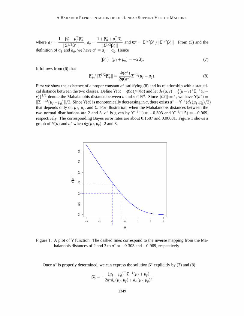
d . Since ‖ω∗‖ = 1, we have ϒ(a∗) =‖Σ−1/2(µ f −µg)‖/2. Since ϒ(a) is monotonically decreasing in a, there exists a∗ = ϒ−1(dΣ(µ f ,µg)/2)that depends only on µ f , µg, and Σ. For illustration, when the Mahalanobis distances between thetwo normal distributions are 2 and 3, a∗ is given by ϒ−1(1) ≈ −0.303 and ϒ−1(1.5) ≈ −0.969,respectively. The corresponding Bayes error rates are about 0.1587 and 0.06681. Figure 1 shows agraph of ϒ(a) and a∗ when dΣ(µ f ,µg)=2 and 3.

−3 −2 −1 0 1 2 3

0.0

0.5

1.0

1.5

2.0

2.5

3.0

a

Υ(a

)

Figure 1: A plot of ϒ function. The dashed lines correspond to the inverse mapping from the Ma-halanobis distances of 2 and 3 to a∗ ≈−0.303 and −0.969, respectively.

Once a∗ is properly determined, we can express the solution β∗ explicitly by (7) and (8):

β∗0 = − (µ f −µg)

>Σ−1(µ f +µg)

2a∗dΣ(µ f ,µg)+dΣ(µ f ,µg)2

1349


and

β∗+ =

2Σ−1(µ f −µg)

2a∗dΣ(µ f ,µg)+dΣ(µ f ,µg)2 .

Thus the optimal hyperplane (3) is

22a∗dΣ(µ f ,µg)+dΣ(µ f ,µg)2

{Σ−1(µ f −µg)

}>{x− 1

2(µ f +µg)

}= 0,

which is equivalent to the Bayes decision boundary given by

{Σ−1(µ f −µg)

}>{x− 1

2(µ f +µg)

}= 0.

This shows that the linear SVM is equivalent to Fisher’s linear discriminant analysis in this setting.In addition, H(β∗) and G(β∗) can be shown to be

G(β∗) =Φ(a∗)

2

[2 (µ f +µg)

>

µ f +µg G22(β∗)

]

and

H(β∗) =φ(a∗)

4(2a∗ +dΣ(µ f ,µg))

[2 (µ f +µg)

>

µ f +µg H22(β∗)

],

where

G22(β∗) = µ f µ>f +µgµ>g +2Σ−

(a∗

dΣ(µ f ,µg)+1

)(µ f −µg)(µ f −µg)

> and

H22(β∗) = µ f µ>f +µgµ>g +2Σ

+2

((a∗

dΣ(µ f ,µg)

)2

+a∗

dΣ(µ f ,µg)− 1

d2Σ(µ f ,µg)

)(µ f −µg)(µ f −µg)

>.

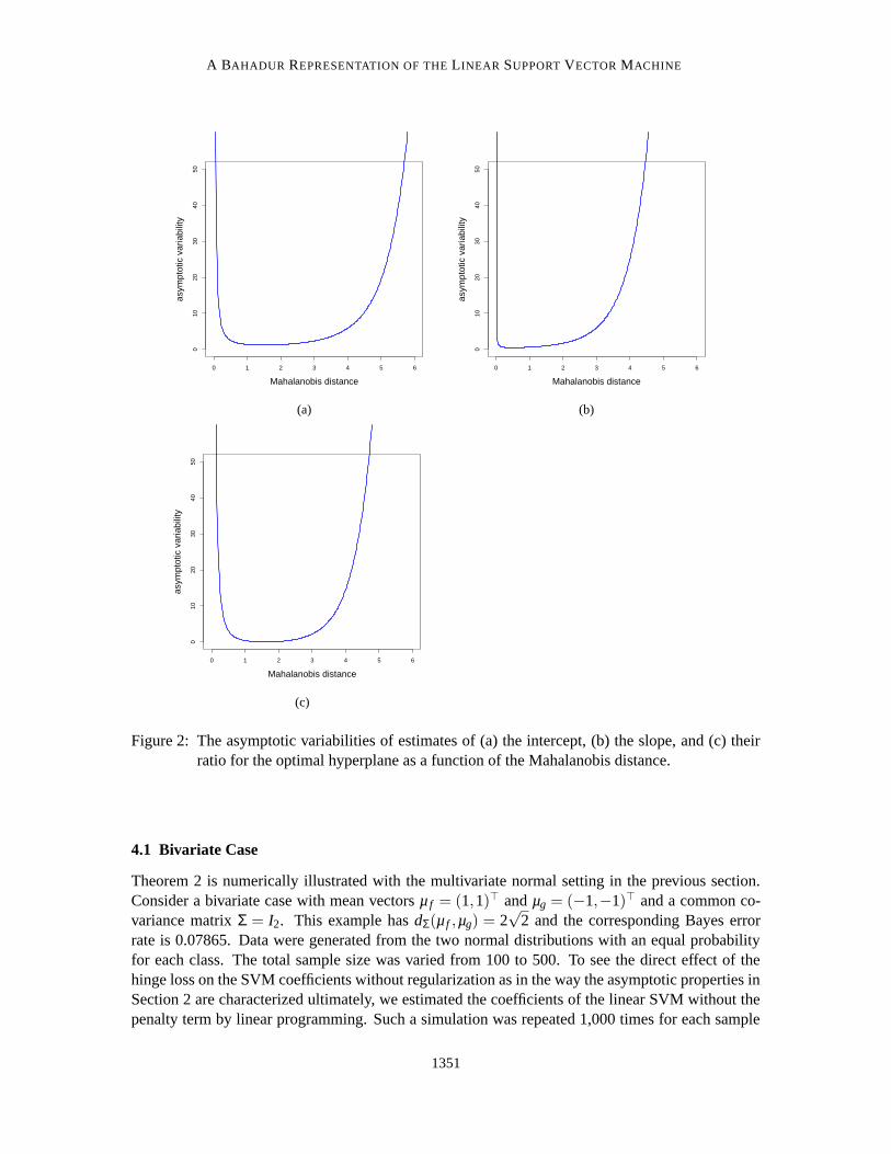
For illustration, we consider the case when d = 1, µ f + µg = 0, and σ = 1. The asymptoticvariabilities of the intercept and the slope for the optimal decision boundary are calculated accordingto Theorem 2. Figure 2 shows the asymptotic variabilities as a function of the Mahalanobis distancebetween the two normal distributions, |µ f −µg| in this case. Also, it depicts the asymptotic varianceof the estimated classification boundary value (−β0/β1) by using the delta method. Although theMahalanobis distance roughly in the range of 1 to 4 would be of practical interest, the plots showa notable trend in the asymptotic variances as the distance varies. When the two classes get veryclose, the variances shoot up due to the difficulty in discriminating them. On the other hand, asthe Mahalanobis distance increases, that is, the two classes become more separated, the variancesbecome increasingly large. A possible explanation for the trend is that the intercept and the slopeof the optimal hyperplane are determined by only a small fraction of data falling into the margins inthis case.

4. Simulation Studies

In this section, simulations are carried out to illustrate the asymptotic results and their potential forfeature selection.

1350


0 1 2 3 4 5 6

010

2030

4050

Mahalanobis distance

asym

ptot

ic v

aria

bilit

y

(a)

0 1 2 3 4 5 6

010

2030

4050


asym

ptot

ic v

aria

bilit

y

(b)

0 1 2 3 4 5 6

010

2030

4050


asym

ptot

ic v

aria

bilit

y

(c)

Figure 2: The asymptotic variabilities of estimates of (a) the intercept, (b) the slope, and (c) theirratio for the optimal hyperplane as a function of the Mahalanobis distance.

4.1 Bivariate Case

Theorem 2 is numerically illustrated with the multivariate normal setting in the previous section.Consider a bivariate case with mean vectors µ f = (1,1)> and µg = (−1,−1)> and a common co-variance matrix Σ = I2. This example has dΣ(µ f ,µg) = 2

√2 and the corresponding Bayes error

rate is 0.07865. Data were generated from the two normal distributions with an equal probabilityfor each class. The total sample size was varied from 100 to 500. To see the direct effect of thehinge loss on the SVM coefficients without regularization as in the way the asymptotic properties inSection 2 are characterized ultimately, we estimated the coefficients of the linear SVM without thepenalty term by linear programming. Such a simulation was repeated 1,000 times for each sample

1351


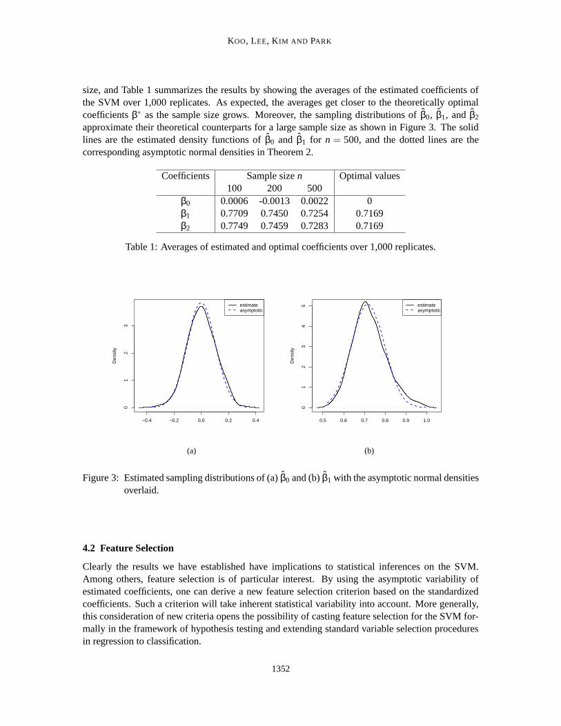
size, and Table 1 summarizes the results by showing the averages of the estimated coefficients ofthe SVM over 1,000 replicates. As expected, the averages get closer to the theoretically optimalcoefficients β∗ as the sample size grows. Moreover, the sampling distributions of β0, β1, and β2

approximate their theoretical counterparts for a large sample size as shown in Figure 3. The solidlines are the estimated density functions of β0 and β1 for n = 500, and the dotted lines are thecorresponding asymptotic normal densities in Theorem 2.

Coefficients Sample size n Optimal values100 200 500

β0 0.0006 -0.0013 0.0022 0β1 0.7709 0.7450 0.7254 0.7169β2 0.7749 0.7459 0.7283 0.7169

Table 1: Averages of estimated and optimal coefficients over 1,000 replicates.

−0.4 −0.2 0.0 0.2 0.4

01

23

Den

sity

estimateasymptotic

(a)

0.5 0.6 0.7 0.8 0.9 1.0

01

23

45

Den

sity

estimateasymptotic

(b)

Figure 3: Estimated sampling distributions of (a) β0 and (b) β1 with the asymptotic normal densitiesoverlaid.

4.2 Feature Selection

Clearly the results we have established have implications to statistical inferences on the SVM.Among others, feature selection is of particular interest. By using the asymptotic variability ofestimated coefficients, one can derive a new feature selection criterion based on the standardizedcoefficients. Such a criterion will take inherent statistical variability into account. More generally,this consideration of new criteria opens the possibility of casting feature selection for the SVM for-mally in the framework of hypothesis testing and extending standard variable selection proceduresin regression to classification.

1352


We investigate the possibility of using the standardized coefficients of β for selection of vari-ables. For practical applications, one needs to construct a reasonable nonparametric estimator ofthe asymptotic variance-covariance matrix, whose entries are defined through line integrals. A sim-ilar technical issue arises in quantile regression. See Koenker (2005) for some suggested varianceestimators in the setting.

For the sake of simplicity in the second set of simulation, we used the theoretical asymptoticvariance in standardizing β and selected those variables with the absolute standardized coefficientexceeding a certain critical value. And we mainly monitored the type I error rate of falsely declaringthe significance of a variable when it is not, over various settings of a mixture of two multivariatenormal distributions. Different combinations of the sample size (n) and the number of variables(d) were tried. For a fixed even d, we set µ f = (1d/2,0d/2)

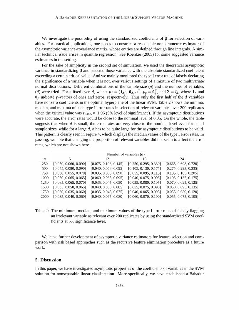
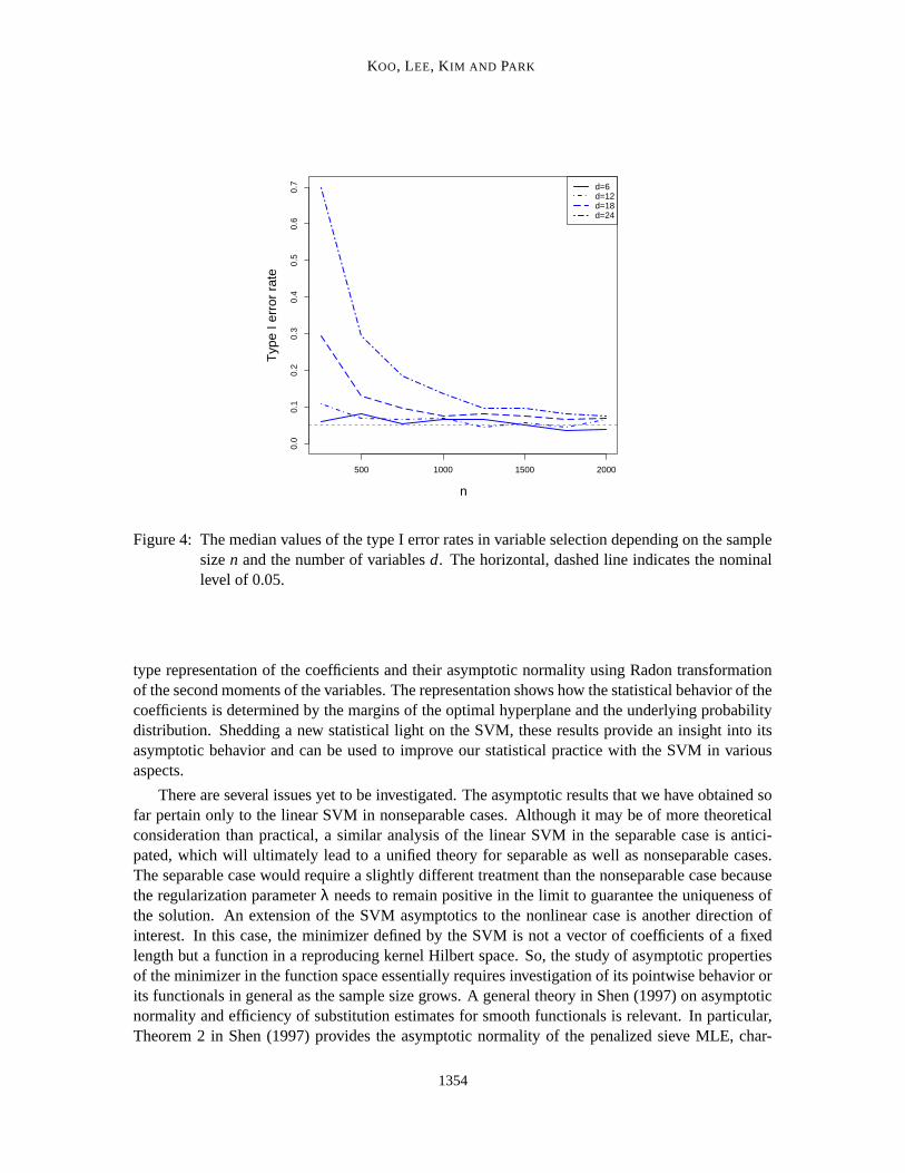
>, µg = 0>d , and Σ = Id , where 1p and0p indicate p-vectors of ones and zeros, respectively. Thus only the first half of the d variableshave nonzero coefficients in the optimal hyperplane of the linear SVM. Table 2 shows the minima,median, and maxima of such type I error rates in selection of relevant variables over 200 replicateswhen the critical value was z0.025 ≈ 1.96 (5% level of significance). If the asymptotic distributionswere accurate, the error rates would be close to the nominal level of 0.05. On the whole, the tablesuggests that when d is small, the error rates are very close to the nominal level even for smallsample sizes, while for a large d, n has to be quite large for the asymptotic distributions to be valid.This pattern is clearly seen in Figure 4, which displays the median values of the type I error rates. Inpassing, we note that changing the proportion of relevant variables did not seem to affect the errorrates, which are not shown here.

Number of variables (d)n 6 12 18 24

250 [0.050, 0.060, 0.090] [0.075, 0.108, 0.145] [0.250, 0.295, 0.330] [0.665, 0.698, 0.720]500 [0.045, 0.080, 0.090] [0.040, 0.068, 0.095] [0.105, 0.130, 0.175] [0.275, 0.293, 0.335]750 [0.030, 0.055, 0.070] [0.035, 0.065, 0.090] [0.055, 0.095, 0.115] [0.135, 0.185, 0.205]

1000 [0.050 ,0.065, 0.065] [0.060, 0.068, 0.095] [0.040, 0.075, 0.095] [0.105, 0.135, 0.175]1250 [0.065, 0.065, 0.070] [0.035, 0.045, 0.050] [0.055, 0.080, 0.105] [0.070, 0.095, 0.125]1500 [0.035, 0.050, 0.065] [0.040, 0.058, 0.085] [0.055, 0.075, 0.090] [0.050, 0.095, 0.135]1750 [0.030, 0.035, 0.060] [0.035, 0.045, 0.075] [0.040, 0.065, 0.095] [0.055, 0.080, 0.120]2000 [0.035, 0.040, 0.060] [0.040, 0.065, 0.080] [0.060, 0.070, 0.100] [0.055, 0.075, 0.105]

Table 2: The minimum, median, and maximum values of the type I error rates of falsely flaggingan irrelevant variable as relevant over 200 replicates by using the standardized SVM coef-ficients at 5% significance level.

We leave further development of asymptotic variance estimators for feature selection and com-parison with risk based approaches such as the recursive feature elimination procedure as a futurework.

5. Discussion

In this paper, we have investigated asymptotic properties of the coefficients of variables in the SVMsolution for nonseparable linear classification. More specifically, we have established a Bahadur

1353


500 1000 1500 2000

0.0

0.1

0.2

0.3

0.4

0.5

0.6

0.7

n

Typ

e I e

rror

rat

e

d=6d=12d=18d=24

Figure 4: The median values of the type I error rates in variable selection depending on the samplesize n and the number of variables d. The horizontal, dashed line indicates the nominallevel of 0.05.

type representation of the coefficients and their asymptotic normality using Radon transformationof the second moments of the variables. The representation shows how the statistical behavior of thecoefficients is determined by the margins of the optimal hyperplane and the underlying probabilitydistribution. Shedding a new statistical light on the SVM, these results provide an insight into itsasymptotic behavior and can be used to improve our statistical practice with the SVM in variousaspects.

There are several issues yet to be investigated. The asymptotic results that we have obtained sofar pertain only to the linear SVM in nonseparable cases. Although it may be of more theoreticalconsideration than practical, a similar analysis of the linear SVM in the separable case is antici-pated, which will ultimately lead to a unified theory for separable as well as nonseparable cases.The separable case would require a slightly different treatment than the nonseparable case becausethe regularization parameter λ needs to remain positive in the limit to guarantee the uniqueness ofthe solution. An extension of the SVM asymptotics to the nonlinear case is another direction ofinterest. In this case, the minimizer defined by the SVM is not a vector of coefficients of a fixedlength but a function in a reproducing kernel Hilbert space. So, the study of asymptotic propertiesof the minimizer in the function space essentially requires investigation of its pointwise behavior orits functionals in general as the sample size grows. A general theory in Shen (1997) on asymptoticnormality and efficiency of substitution estimates for smooth functionals is relevant. In particular,Theorem 2 in Shen (1997) provides the asymptotic normality of the penalized sieve MLE, char-

1354


acterization of which bears a close resemblance with function estimation for the nonlinear case.However, the theory was developed under the assumption of the differentiability of the loss, andit has to be modified for proper theoretical analysis of the SVM. As in the approach for the linearcase presented in this paper, one may get around the non-differentiability issue of the hinge loss byimposing appropriate regularity conditions to ensure that the minimizer is unique and the expectedloss is differentiable and locally quadratic around the minimizer.

Consideration of these extensions will lead to a more complete picture of the asymptotic behav-ior of the SVM solution.

6. Proofs

In this section, we present technical lemmas and prove the main results.

6.1 Technical Lemmas

Lemma 1 shows that there is a finite minimizer of L(β), which is useful in proving the uniqueness ofthe minimizer in Lemma 6. In fact, the existence of the first moment of X is sufficient for Lemmas1, 2, and 4. However, (A1) is needed for the existence and continuity of H(β) in the proof of otherlemmas and theorems.

Lemma 1 Suppose that (A1) and (A2) are satisfied. Then L(β) → ∞ as ‖β‖→ ∞ and the existenceof β∗ is guaranteed.

Proof. Without loss of generality, we may assume that x0 = 0 in (A2) and B(0,δ0) ⊂ X . For anyε > 0,

L(β) = π+

Z

X[1− x>β]+ f (x)dx+π−

Z

X[1+h(x;β)]+g(x)dx

≥ π+

Z

X{h(x;β) ≤ 0}(1−h(x;β)) f (x)dx+π−

Z

X{h(x;β) ≥ 0}(1+h(x;β))g(x)dx

≥ π+

Z

X{h(x;β) ≤ 0}(−h(x;β)) f (x)dx+π−

Z

X{h(x;β) ≥ 0}h(x;β)g(x)dx

≥Z

X|h(x;β)|min(π+ f (x),π−g(x))dx

≥ C1 min(π+,π−)Z

B(0,δ0)|h(x;β)|dx

= C1 min(π+,π−)‖β‖Z

B(0,δ0)|h(x;w)|dx

≥ C1 min(π+,π−)‖β‖vol({|h(x;w)| ≥ ε}∩B(0,δ0))ε,

where w = β/‖β‖ and vol(A) denotes the volume of a set A.

1355


Note that −1 ≤ w0 ≤ 1. For 0 ≤ w0 < 1 and 0 < ε < 1,

vol({|h(x;w)| ≥ ε}∩B(0,δ0))

≥ vol({h(x;w) ≥ ε}∩B(0,δ0))

= vol

({x>w+/

√1−w2

0 ≥ (ε−w0)/√

1−w20

}∩B(0,δ0)

)

≥ vol

({x>w+/

√1−w2

0 ≥ ε}∩B(0,δ0)

)≡V (δ0,ε)

since (ε−w0)/√

1−w20 ≤ ε. When −1 < w0 < 0, we obtain

volB(h(x;w) ≤−ε) ≥V (δ0,ε)

in a similar way. Note that V (δ0,ε) is independent of β and V (δ0,ε) > 0 for some ε < δ0. Conse-quently, L(β) ≥C1 min(π+,π−)‖β‖V (δ0,ε)ε → ∞ as ‖β‖→ ∞. The case w0 = ±1 is trivial.

Since the hinge loss is convex, L(β) is convex in β. Since L(β) → ∞ as ‖β‖ → ∞, the set,denoted by M , of minimizers of L(β) forms a bounded connected set. The existence of the solutionβ∗ of L(β) easily follows from this. �

In Lemmas 2 and 3, we obtain explicit forms of S(β) and H(β) for non-constant decision func-tions.

Lemma 2 Assume that (A1) is satisfied. If β+ 6= 0, then we have

∂L(β)

∂β j= S(β) j

for 0 ≤ j ≤ d.

Proof. It suffices to show that

∂∂β j

Z

X[1−h(x;β)]+ f (x)dx = −

Z

X{h(x;β) ≤ 1}x j f (x)dx.

Define ∆(t) = [1−h(x;β)− t x j]+− [1−h(x;β)]+. Let t > 0.First, consider the case x j > 0. Then,

∆(t) =

0 if h(x;β) > 1h(x;β)−1 if 1− t x j < h(x;β) ≤ 1−tx j if h(x;β) ≤ 1− tx j.

Observe thatZ

X∆(t){x j > 0} f (x)dx =

Z

X{1− tx j < h(x;β) ≤ 1}(h(x;β)−1) f (x)dx

−tZ

X{h(x;β) ≤ 1− t x j, x j > 0}x j f (x)dx

and that∣∣∣∣1t

Z

X{1− tx j < h(x;β) ≤ 1}(h(x;β)−1) f (x)dx

∣∣∣∣≤Z

X{1− tx j < h(x;β) ≤ 1}x j f (x)dx.

1356


By Dominated Convergence Theorem,

limt↓0

Z

X{1− tx j < h(x;β) ≤ 1}x j f (x)dx =

Z

X{h(x;β) = 1}x j f (x)dx = 0

andlimt↓0

Z

X{h(x;β) ≤ 1− t x j, x j > 0}x j f (x)dx =

Z

X{h(x;β) ≤ 1, x j > 0}x j f (x)dx.

Hence

limt↓0

1t

Z

X∆(t){x j > 0} f (x)dx = −

Z

X{h(x;β) ≤ 1, x j > 0}x j f (x)dx. (9)

Now assume that x j < 0. Then,

∆(t) =

0 if h(x;β) > 1− t x j

1−h(x;β)− tx j if 1 < h(x;β) ≤ 1− t x j

−tx j if h(x;β) ≤ 1.

In a similar fashion, one can show that

limt↓0

1t

Z

X∆(t){x j < 0} f (x)dx = −

Z

X{h(x;β) ≤ 1, x j < 0}x j f (x)dx. (10)

Combining (9) and (10), we have shown that

limt↓0

1t

Z

X∆(t) f (x)dx = −

Z

X{h(x;β) ≤ 1}x j f (x)dx.

The proof for the case t < 0 is similar. �

The proof of Lemma 3 is based on the following identityZ

δ(Dt +E)T (t)dt =1|D|T (−E/D) (11)

for constants D and E. This identity follows from the fact that δ(at) = δ(t)/|a| andR

δ(t−a)T (t)dt =T (a) for a constant a.

Lemma 3 Suppose that (A1) is satisfied. Under the condition that β+ 6= 0, we have

∂2L(β)

∂β j∂βk= H(β) jk,

for 0 ≤ j,k ≤ d.

Proof. DefineΨ(β) =

Z

X{x>β+ < 1−β0}s(x)dx

for a continuous and integrable function s defined on X . Without loss of generality, we may assumethat β1 6= 0. It is sufficient to show that for 0 ≤ j,k ≤ d,

∂2

∂β j∂βk

Z

X[1−h(x;β)]+ f (x)dx =

Z

Xδ(1−h(x;β))x jxk f (x)dx.

1357


Define X− j = {(x1, . . . ,x j−1,x j+1, . . . ,xd) : (x1, . . . ,xd) ∈ X } and X j = {x j : (x1, . . . ,xd) ∈ X }.Observe that

∂Ψ(β)

∂β0= − 1

|β1|

Z

X−1

s

(1−h(x;β)+β1x1

β1,x2, . . . ,xd

)dx−1 (12)

and that for k 6= 1,

∂Ψ(β)

∂βk= − 1

|β1|

Z

X−1

xks

(1−h(x;β)+β1x1

β1,x2, . . . ,xd

)dx−1. (13)

If βp = 0 for any p 6= 1, then

∂Ψ(β)

∂β1= −1−β0

β1|β1|

Z

X−1

s

(1−β0

β1,x2, . . . ,xd

)dx−1. (14)

If there is p 6= 1 with βp 6= 0, then we have

∂Ψ(β)

∂β1= − 1

|βp|

Z

X−p

x1s

(x1, . . . ,xp−1,

1−h(x;β)+βpxp

βp,xp+1, . . . ,xd

)dx−p. (15)

Choose D = β1, E = x>β−β1x1 −1, t = x1 in (11). It follows from (13) and (15) that

∂Ψ(β)

∂βk= − 1

|β1|

Z

X−1

xks

(1−h(x;β)+β1x1

β1,x2, . . . ,xd

)dx−1 (16)

= −Z

X−1

Z

X1

xks(x)δ(h(x;β)−1)dx1dx−1

= −Z

Xδ(1−h(x;β))xks(x)dx.

Similarly, we have∂Ψ(β)

∂β0= −

Z

Xδ(1−h(x;β))s(x)dx (17)

by (12).Choosing D = β1, E = β0 −1, t = x1 in (11), we have

Z

X1

δ(β1x1 −1+β0)x1s(x)dx1 =1

|β1|

(1−β0

β1

)s

(1−β0

β1,x2, . . . ,xd

)

by (14). This implies (16) for k = 1. The desired result now follows from (16) and (17). �

The following lemma asserts that the optimal decision function is not a constant under thecondition that the centers of two classes are separated.

Lemma 4 Suppose that (A1) is satisfied. Then (A3) implies that β∗+ 6= 0.

Proof. Suppose thatZ

X{xi∗ ≥ G−

i∗}xi∗g(x)dx <Z

X{xi∗ ≤ F+

i∗ }xi∗ f (x)dx (18)

in (A3). We will show that

minβ0

L(β0,0, . . .0) > minβ0,βi∗>0

L(β0,0, . . . ,0,βi∗ ,0, . . . ,0), (19)

1358


implying that β∗+ 6= 0. Henceforth, we will suppress β’s that are equal to zero in L(β). The popula-

tion minimizer (β∗0,β∗

i∗) is given by the minimizer of

L(β0,βi∗) = π+

Z

X[1−β0 −βi∗xi∗ ]+ f (x)dx+π−

Z

X[1+β0 +βi∗xi∗ ]+g(x)dx.

First, consider the case βi∗ = 0.

L(β0) =

π−(1+β0), β0 > 11+(π−−π+)β0, −1 ≤ β0 ≤ 1π+(1−β0), β0 < −1

with its minimummin

β0

L(β0) = 2min(π+,π−) . (20)

Now consider the case βi∗ > 0, where

L(β0,βi∗) = π+

Z

X

{xi∗ ≤

1−β0

βi∗

}(1−β0 −βi∗xi∗) f (x)dx

+π−

Z

X

{xi∗ ≥

−1−β0

βi∗

}(1+β0 +βi∗xi∗)g(x)dx.

Let β0 denote the minimizer of L(β0,βi∗) for a given βi∗ . Note that ∂L(β0,βi∗)/∂β0 is given as

∂L(β0,βi∗)

∂β0(21)

= −π+

Z

X

{xi∗ ≤

1−β0

βi∗

}f (x)dx+π−

Z

X

{xi∗ ≥

−1−β0

βi∗

}g(x)dx,

which is monotonic increasing in β0 with limβ0→−∞∂L(β0,βi∗ )

∂β0→−π+ and limβ0→∞

∂L(β0,βi∗ )∂β0

→ π−.

Hence β0 exists for a given βi∗ .When π− < π+, we can easily check that F+

i∗ < ∞ and G−i∗ = −∞. F+

i∗ and G−i∗ may not be

determined uniquely, meaning that there may exist an interval with probability zero. There is nosignificant change in the proof under the assumption that F+

i∗ and G−i∗ are unique. Note that

1− β0

βi∗≤ F+

i∗

by definition of F+i∗ and (21). Then,

−1− β0

βi∗≤ F+

i∗ − 2βi∗

→−∞ as βi∗ → 0,

and1− β0

βi∗→ F+

i∗ as βi∗ → 0.

¿From (18),

π−

Z

Xxi∗g(x)dx < π+

Z

X{xi∗ ≤ F+

i∗ }xi∗ f (x)dx. (22)

1359


Now consider the minimum of L(β0,βi∗) with respect to βi∗ > 0. From (21),

L(β0,βi∗) (23)

= π+

Z

X

{xi∗ ≤

1− β0

βi∗

}(1− β0 −βi∗xi∗) f (x)dx

+π−

Z

X

{xi∗ ≥

−1− β0

βi∗

}(1+ β0 +βi∗xi∗)g(x)dx

= 2π−

Z

X

{xi∗ ≥

−1− β0

βi∗

}g(x)dx

+βi∗

(π−

Z

X

{xi∗ ≥

−1− β0

βi∗

}xi∗g(x)dx−π+

Z

X

{xi∗ ≤

1− β0

βi∗

}xi∗ f (x)dx

)

By (22), it can be easily seen that the second term in (23) is negative for sufficiently small βi∗ > 0,implying

L(β0,βi∗) < 2π− for some βi∗ > 0.

If π− > π+, then F+i∗ = ∞ and G−

i∗ > −∞. Similarly, it can be checked that

L(β0,βi∗) < 2π+ for some βi∗ > 0.

Suppose that π− = π+. Then it can be verified that

1− β0

βi∗→ ∞ as βi∗ → 0,

and−1− β0

βi∗→−∞ as βi∗ → 0.

In this case, L(β0,βi∗) < 1.Hence, under (18), we have shown that

L(β0,βi∗) < 1 for some βi∗ > 0.

This, together with (20), implies (19). For the second case in (A3), the same arguments hold withβi∗ < 0. �

Note that (A1) implies that H is well-defined and continuous in its argument. (A4) ensures thatH(β) is positive definite around β∗ and thus we have a lower bound result in Lemma 5.

Lemma 5 Under (A1), (A3) and (A4),

β>H(β∗)β ≥C4‖β‖2,

where C4 may depend on β∗.

1360


Proof. Since the proof for the case d = 1 is trivial, we consider the case d ≥ 2 only. Observe that

β>H(β∗)β = E

(δ(1−Y h(X ;β∗))h2(X ;β)

)

= π+

Z

Xδ(1−h(x;β∗))h2(x;β) f (x)dx+π−

Z

Xδ(1+h(x;β∗))h2(x;β)g(x)dx

= π+(R h2 f )(1−β∗0,β

∗+)+π−(R h2g)(1+β∗

0,−β∗+)

= π+(R h2 f )(1−β∗0,β

∗+)+π−(R h2g)(−1−β∗

0,β∗+).

The last equality follows from the homogeneity of Radon transform.

Recall that β∗+ 6= 0 by Lemma 4. Without loss of generality, we assume that j∗ = 1 in (A4). Let

A1β+ = a = (a1, . . . ,ad) and z = (A1x)/‖β∗+‖. Given u = (u2, . . . ,ud), let u∗ =

((1−β∗

0)/‖β∗+‖,u

).

Define Z = {z = (A1x)/‖β∗+‖ : x ∈ X } and U = {u : u j = ‖β∗

+‖z j for j = 2, . . . ,d, and z ∈ Z}. Notethat detA1 = 1, du = ‖β∗

+‖d−1dz2 . . .dzd ,

‖β∗+‖A>

1 z∣∣∣z1=(1−β∗

0)/‖β∗+‖2

= A>1

(1−β∗0)/‖β∗

+‖‖β∗

+‖z2...

‖β∗+‖zd

= A>

1 u∗

and

β0 +‖β∗+‖a>z

∣∣∣z1=(1−β∗

0)/‖β∗+‖2

= β0 +‖β∗+‖(

a1(1−β∗0)/‖β∗

+‖2 +d

∑j=2

a jz j

)

= β0 +a1(1−β∗0)/‖β∗

+‖+‖β∗+‖

d

∑j=2

a jz j.

Using the transformation A1, we have

(R h2 f )(1−β∗0,β

∗+)

=Z

Zδ(

1−β∗0 −‖β∗

+‖(A1β∗+)>z

)h2(‖β∗

+‖A>1 z;β

)f(‖β∗

+‖A>1 z)‖β∗

+‖ddz

=Z

Zδ(

1−β∗0 −‖β∗

+‖2e>1 z)(

β0 +‖β∗+‖(A1β+)>z

)2f(‖β∗

+‖A>1 z)‖β∗

+‖ddz

=Z

Zδ(1−β∗

0 −‖β∗+‖2z1

)(β0 +‖β∗

+‖a>z)2

f(‖β∗

+‖A>1 z)‖β∗

+‖ddz

=1

‖β∗+‖

Z

U

(β0 +a1(1−β∗

0)/‖β∗+‖+

d

∑j=2

a ju j

)2f (A>

1 u∗)du.

1361


The last equality follows from the identity (11). Let D+∗ =

{u : A>

1 u∗ ∈ D+}

. By (A4), there existsa constant C2 > 0 and a rectangle D+

∗ on which f (A>1 u∗) ≥C2 for u ∈ D+

∗ . Then

(R h2 f )(1−β∗0,β

∗+)

≥ 1‖β∗

+‖

Z

D+∗

(β0 +a1(1−β∗

0)/‖β∗+‖+

d

∑j=2

a ju j

)2f (A>

1 u∗)du

≥ 1‖β∗

+‖·C2

Z

D+∗

(β0 +a1(1−β∗

0)/‖β∗+‖+

d

∑j=2

a ju j

)2du

=1

‖β∗+‖

·C2 ·vol(D+∗ )Eu

(β0 +a1(1−β∗

0)/‖β∗+‖+

d

∑j=2

a jU j

)2

=1

‖β∗+‖

·C2 ·vol(D+∗ ){(

β0 +a1(1−β∗0)/‖β∗

+‖+Eu

d

∑j=2

a jU j

)2+V

u(d

∑j=2

a jU j)},

where U j for j = 2, . . . ,d are independent and uniform random variables defined on D+∗ , and E

u andV

u denote the expectation and variance with respect to the uniform distribution.

Letting mi = (li + vi)/2, we have

(R h2 f )(1−β∗0,β

∗+) (24)

≥ 1‖β∗

+‖·C2 ·vol(D+

∗ ){(

β0 +a1(1−β∗0)/‖β∗

+‖+d

∑j=2

a jm j

)2+ min

2≤ j≤dV

u(U j)d

∑j=2

a2j

}.

Similarly, it can be shown that

(R h2g)(−1−β∗0,β

∗+) (25)

≥ 1‖β∗

+‖·C3 ·vol(D−

∗ ){(

β0 −a1(1+β∗0)/‖β∗

+‖+d

∑j=2

a jm j

)2+ min

2≤ j≤dV

u(U j)d

∑j=2

a2j

},

where D−∗ =

{u : A>

1

((−1−β∗

0)/‖β∗+‖,u

)∈ D−

}.

1362


Combining (24)-(25) and letting C5 = 2/‖β∗+‖min

(π+C2 ·vol(D+

∗ ),π−C3 ·vol(D−∗ ))

and C6 =

min(

1,min2≤ j≤d Vu(U j)

), we have

β>H(β∗)β

≥ π+

‖β∗+‖

·C2 ·vol(D+∗ ){(

β0 +a1(1−β∗0)/‖β∗

+‖+d

∑j=2

a jm j

)2+ min

2≤ j≤dV

u(U j)d

∑j=2

a2j

}

+π−‖β∗

+‖·C3 ·vol(D−

∗ ){(

β0 −a1(1+β∗0)/‖β∗

+‖+d

∑j=2

a jm j

)2+ min

2≤ j≤dV

u(U j)d

∑j=2

a2j

}

≥ C5C6

{(β0 +a1(1−β∗

0)/‖β∗+‖+

d

∑j=2

a jm j

)2

+(

β0 −a1(1+β∗0)/‖β∗

+‖+d

∑j=2

a jm j

)2+2

d

∑j=2

a2j

}/2

= C5C6

{(β0 +a1(1−β∗

0)/‖β∗+‖)2

+(

β0 −a1(1+β∗0)/‖β∗

+‖)2

+4(

β0 −a1β∗0/‖β∗

+‖) d

∑j=2

a jm j +2( d

∑j=2

a jm j

)2+2

d

∑j=2

a2j

}/2.

Note that

( d

∑j=2

a jm j

)2+2(

β0 −a1β∗0/‖β∗

+‖) d

∑j=2

a jm j

=( d

∑j=2

a jm j +β0 −a1β∗0/‖β∗

+‖)2

−(

β0 −a1β∗0/‖β∗

+‖)2

and(

β0 +a1(1−β∗0)/‖β∗

+‖)2

+(

β0 −a1(1+β∗0)/‖β∗

+‖)2

−2(

β0 −a1β∗0/‖β∗

+‖)2

= 2a21/‖β∗

+‖2.

Thus, the lower bound of β>H(β∗)β except for the constant C5C6 allows the following quadraticform in terms of β0,a1, . . . ,ad . Let

Q(β0,a1, . . . ,ad) = a21/‖β∗

+‖2 +( d

∑j=2

a jm j +β0 −a1β∗0/‖β∗

+‖)2

+d

∑j=2

a2j .

Obviously Q(β0,a1, . . . ,ad)≥ 0 and Q(β0,a1, . . . ,ad) = 0 implies that a1 = . . . = ad = 0 and β0 = 0.Therefore Q is positive definite. Letting ν1 > 0 be the smallest eigenvalue of the matrix correspond-ing to Q, we have proved

β>H(β∗)β ≥ C5C6ν1(β20 +

d

∑j=1

a2j) = C5C6ν1(β2

0 +d

∑j=1

β2j).

The last equality follows from the fact that A1β+ = a and the transformation A1 preserves the norm.With the choice of C4 = C5C6ν1 > 0, the result follows. �

1363


Lemma 6 Suppose that (A1)-(A4) are met. Then L(β) has a unique minimizer.

Proof. By Lemma 1, we may choose any minimizer β∗ ∈ M . By Lemma 4 and 5, H(β) is positivedefinite at β∗. Then L(β) is locally strictly convex at β∗, so that L(β) has a local minimum at β∗.Hence the minimizer of L(β) is unique. �

6.2 Proof of Theorems 1 and 2

For fixed θ ∈ Rd+1, define

Λn(θ) = n(

lλ,n(β∗ +θ/√

n)− lλ,n(β∗))

andΓn(θ) = EΛn(θ).

Observe that

Γn(θ) = n(L(β∗ +θ/

√n)−L(β∗)

)+

λ2

(‖θ+‖2 +2

√nβ∗

+>θ+

).

By Taylor series expansion of L around β∗, we have

Γn(θ) =12

θ>H(β)θ+λ2

(‖θ+‖2 +2

√nβ∗

+>θ+

),

where β = β∗+(t/√

n)θ for some 0 < t < 1. Define D jk(α) = H(β∗+α) jk −H(β∗) jk for 0 ≤ j,k ≤d. Since H(β) is continuous in β, there exists δ1 > 0 such that |D jk(α)| < ε1 if ‖α‖ < δ1 for anyε1 > 0 and all 0 ≤ j,k ≤ d. Then, as n → ∞,

12

θ>H(β)θ =12

θ>H(β∗)θ+o(1).

It is because for sufficiently large n such that ‖(t/√n)θ‖ < δ1,

∣∣∣θ>(

H(β)−H(β∗))

θ∣∣∣ ≤ ∑

j,k

|θ j||θk|∣∣∣∣D jk

(t√n

θ)∣∣∣∣

≤ ε1 ∑j,k

|θ j||θk| ≤ 2ε1‖θ‖2.

Together with the assumption that λ = o(n−1/2), we have

Γn(θ) =12

θ>H(β∗)θ+o(1).

Define Wn = −∑ni=1 ζiY iX i where ζi =

{Y ih(X i;β∗) ≤ 1

}. Then 1√

nWn follows asymptotically

N(

0,nG(β∗))

by central limit theorem. Note that

E

(ζiY iX i

)= 0 and E

(ζiY iX i(ζiY iX i)>

)= E

(ζiX i(X i)>

). (26)

1364


Recall that β∗ is characterized by S(β∗) = 0 implying the first part of (26). If we define

Ri,n(θ) =[1−Y ih(X i;β∗ +θ/

√n)]+−[1−Y ih(X i;β∗)

]+

+ζiY ih(X i;θ/√

n),

then we see that

Λn(θ) = Γn(θ)+W>n θ/

√n+

n

∑i=1

(Ri,n(θ)−ERi,n(θ)

)

and ∣∣∣Ri,n(θ)∣∣∣≤∣∣∣h(X i;θ)/

√n∣∣∣U(∣∣∣h(X i;θ)/

√n∣∣∣)

, (27)

where

U(t) ={∣∣∣1−Y ih(X i;β∗)

∣∣∣≤ t}

for t ∈ R.

To verify (27), let ζ = {a ≤ 1} and R = [1− z]+− [1−a]+ +ζ(z−a). If a > 1, then R = (1− z){z ≤1}; otherwise, R = (z−1){z > 1}. Hence,

R = (1− z){a > 1,z ≤ 1}+(z−1){a < 1,z > 1} (28)

≤ |z−a|{a > 1,z ≤ 1}+ |z−a|{a < 1,z > 1}= |z−a|

({a > 1,z ≤ 1}+{a < 1,z > 1}

)

≤ |z−a|{|1−a| ≤ |z−a|}.

Choosing z = Y ih(X i;β∗ +θ/√

n) and a = Y ih(X i;β∗) in (28) yields (27).Since cross-product terms in E(∑i(Ri,n −ERi,n))

2 cancel out, we obtain from (27) that for eachfixed θ,

n

∑i=1

E

(|Ri,n(θ)−ERi,n(θ)|2

)≤

n

∑i=1

E(Ri,n(θ)2)

≤n

∑i=1

E

((h(X i;θ)/

√n)2

U(|h(X i;θ)/

√n|))

≤n

∑i=1

E

((1+‖X i‖2)‖θ‖2/n U

(√1+‖X i‖2‖θ‖/

√n

))

= ‖θ‖2E

((1+‖X‖2) U

(√1+‖X‖2‖θ‖/

√n

)).

(A1) implies that E(‖X‖2

)< ∞. Hence, for any ε > 0, choose C7 such that E

((1 +‖X‖2){‖X‖ >

C7})

< ε/2. Then

E

((1+‖X‖2) U

(√1+‖X‖2‖θ‖/

√n

))

≤ E

((1+‖X‖2){‖X‖ > C7}

)+(1+C2

7)P

(U

(√1+C2

7‖θ‖/√

n

))

1365


By (A1), the distribution of X is not degenerate, which in turn implies that limt↓0 P(U(t)) = 0. We

can take a large N such that P

(U

(√1+C2

7‖θ‖/√n

))< ε/(2(1 +C2

7)) for n ≥ N. This proves

thatn

∑i=1

E

(|Ri,n(θ)−ERi,n(θ)|2

)→ 0

as n → ∞. Thus, for each fixed θ,

Λn(θ) =12

θ>H(β∗)θ+W>n θ/

√n+oP(1).

Let ηn = −H(β∗)−1Wn/√

n. By Convexity Lemma in Pollard (1991), we have

Λn(θ) =12(θ−ηn)

>H(β∗)(θ−ηn)−12

η>n H(β∗)ηn + rn(θ),

where, for each compact set K in Rd+1,

supθ∈K

|rn(θ)| → 0 in probability.

Because ηn converges in distribution, there exists a compact set K containing Bε, where Bε is aclosed ball with center ηn and radius ε with probability arbitrarily close to one. Hence we have

∆n = supθ∈Bε

|rn(θ)| → 0 in probability. (29)

For examination of the behavior of Λn(θ) outside Bε, consider θ = ηn + γv, with γ > ε and v, aunit vector and a boundary point θ∗ = ηn + εv. By Lemma 5, convexity of Λn, and the definition of∆n, we have

εγ

Λn(θ)+

(1− ε

γ

)Λn(ηn) ≥ Λn(θ∗)

≥ 12(θ∗−ηn)

>H(β∗)(θ∗−ηn)−12

η>n H(β∗)ηn −∆n

≥ C4

2ε2 +Λn(ηn)−2∆n,

implying that

inf‖θ−ηn‖>ε

Λn(θ) ≥ Λn(ηn)+

(C4

2ε2 −2∆n

).

By (29), we can take ∆n so that 2∆n < C4ε2/4 with probability tending to one. So the minimumof Λn cannot occur at any θ with ‖θ−ηn‖ > ε. Hence, for each ε > 0 and θλ,n =

√n(βλ,n −β∗),

P

(‖θλ,n −ηn‖ > ε

)→ 0.

This completes the proof of Theorems 1 and 2. �

Acknowledgments

The authors are grateful to Wolodymyr Madych for personal communications on Radon transform.This research was supported by a Korea Research Foundation Grant funded by the Korean govern-ment (MOEHRD, Basic Research Promotion Fund) (KRF-2005-070-C00020).

1366


References

R. R. Bahadur. A note on quantiles in large samples. Annals of Mathematical Statistics, 37:577–580,1966.

P. L. Bartlett, M. I. Jordan, and J. D. McAuliffe. Convexity, classification, and risk bounds. Journalof the American Statististical Association, 101:138–156, 2006.

G. Blanchard, O. Bousquet, and P. Massart. Statistical performance of support vector machines.The Annals of Statistics, 36:489–531, 2008.

P. Chaudhuri. Nonparametric estimates of regression quantiles and their local Bahadur representa-tion. The Annals of Statistics, 19:760–777, 1991.

C. Cortes and V. Vapnik. Support-vector networks. Machine Learning, 20:273–297, 1995.

N. Cristianini and J. Shawe-Taylor. An Introduction to Support Vector Machines and Other Kernel-based Learning Methods. Cambridge University Press, Cambridge, 2000.

S. R. Deans. The Radon Transform and Some of Its Applications. Krieger Publishing Company,Florida, 1993.

I. Guyon and A. Elisseeff. Introduction to variable and feature selection. Journal of MachineLearning Research, 3:1157–1182, 2003.

I. Guyon, J. Weston, S. Barnhill, and V. Vapnik. Gene selection for cancer classification usingsupport vector machines. Machine Learning, 46:389–422, 2002.

A. B. Ishak and B. Ghattas. An efficient method for variable selection using svm-based criteria.Preprint, Institut de Mathematiques de Luminy, 2005.

R. Koenker. Quantile Regression. Econometric Society Monographs. Cambridge University Press,2005.

Y. Lin. Some asymptotic properties of the support vector machine. Technical report 1029, Depart-ment of Statistics, University of Wisconsin-Madison, 2000.

Y. Lin. A note on margin-based loss functions in classification. Statististics and Probability Letters,68:73–82, 2002.

F. Natterer. The Mathematics of Computerized Tomography. Wiley & Sons, New York, 1986.

D. Pollard. Asymptotics for least absolute deviation regression estimators. Econometric Theory, 7:186–199, 1991.

A. G. Ramm and A. I. Katsevich. The Radon Transform and Local Tomography. CRC Press, BocaRaton, 1996.

B. Scholkopf and A. Smola. Learning with Kernels - Support Vector Machines, Regularization,Optimization and Beyond. MIT Press, 2002.

1367


J. C. Scovel and I. Steinwart. Fast rates for support vector machines using gaussian kernels. TheAnnals of Statistics, 35:575–607, 2007.

X. Shen. On methods of sieves and penalization. The Annals of Statistics, 25:2555–2591, 1997.

I. Steinwart. Consistency of support vector machines and other regularized kernel machines. IEEETransactions on Information Theory, 51:128–142, 2005.

V. Vapnik. The Nature of Statistical Learning Theory. Springer, New York, 1996.

T. Zhang. Statistical behavior and consistency of classification methods based on convex risk mini-mization. The Annals of Statistics, 32:56–84, 2004.

1368

A Bahadur Representation of the Linear Support Vector...

Documents

Transcript of A Bahadur Representation of the Linear Support Vector...