9 Nonseasonal ARIMA
60
Forecasting using 9. Non-seasonal ARIMA models OTexts.com/fpp/8/ Forecasting using R 1 Rob J Hyndman
-
Upload
justinlondon -
Category
Documents
-
view
224 -
download
1
description
9 Nonseasonal ARIMA
Transcript of 9 Nonseasonal ARIMA
Forecasting using
9. Non-seasonal ARIMA models
OTexts.com/fpp/8/
Forecasting using R 1
Rob J Hyndman
Outline
1 Non-seasonal ARIMA models
2 Estimation and order selection
3 ARIMA modelling in R
Forecasting using R Non-seasonal ARIMA models 2
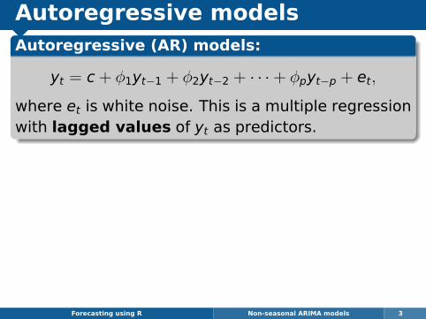
Autoregressive modelsAutoregressive (AR) models:
yt = c+ φ1yt−1 + φ2yt−2 + · · ·+ φpyt−p + et,
where et is white noise. This is a multiple regressionwith lagged values of yt as predictors.
Forecasting using R Non-seasonal ARIMA models 3
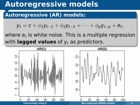
Autoregressive modelsAutoregressive (AR) models:
yt = c+ φ1yt−1 + φ2yt−2 + · · ·+ φpyt−p + et,
where et is white noise. This is a multiple regressionwith lagged values of yt as predictors.
AR(1)
Time
0 20 40 60 80 100
78
910
1112
13
AR(2)
Time
0 20 40 60 80 100
1618
2022
24
Forecasting using R Non-seasonal ARIMA models 3
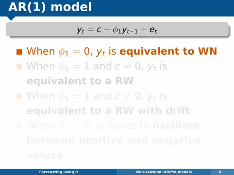
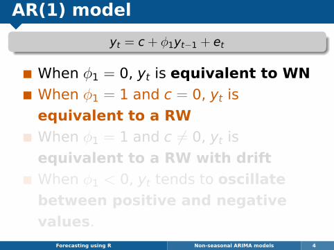
AR(1) model
yt = c+ φ1yt−1 + et
When φ1 = 0, yt is equivalent to WN
When φ1 = 1 and c = 0, yt is
equivalent to a RW
When φ1 = 1 and c 6= 0, yt is
equivalent to a RW with drift
When φ1 < 0, yt tends to oscillate
between positive and negative
values.
Forecasting using R Non-seasonal ARIMA models 4
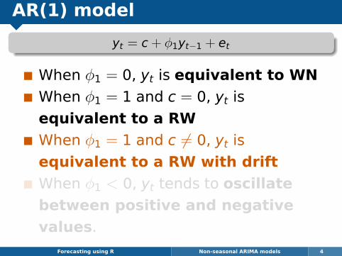
AR(1) model
yt = c+ φ1yt−1 + et
When φ1 = 0, yt is equivalent to WN
When φ1 = 1 and c = 0, yt is
equivalent to a RW
When φ1 = 1 and c 6= 0, yt is
equivalent to a RW with drift
When φ1 < 0, yt tends to oscillate
between positive and negative
values.
Forecasting using R Non-seasonal ARIMA models 4
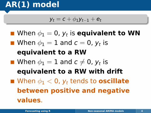
AR(1) model
yt = c+ φ1yt−1 + et
When φ1 = 0, yt is equivalent to WN
When φ1 = 1 and c = 0, yt is
equivalent to a RW
When φ1 = 1 and c 6= 0, yt is
equivalent to a RW with drift
When φ1 < 0, yt tends to oscillate
between positive and negative
values.
Forecasting using R Non-seasonal ARIMA models 4
AR(1) model
yt = c+ φ1yt−1 + et
When φ1 = 0, yt is equivalent to WN
When φ1 = 1 and c = 0, yt is
equivalent to a RW
When φ1 = 1 and c 6= 0, yt is
equivalent to a RW with drift
When φ1 < 0, yt tends to oscillate
between positive and negative
values.
Forecasting using R Non-seasonal ARIMA models 4
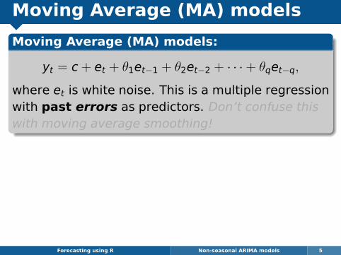
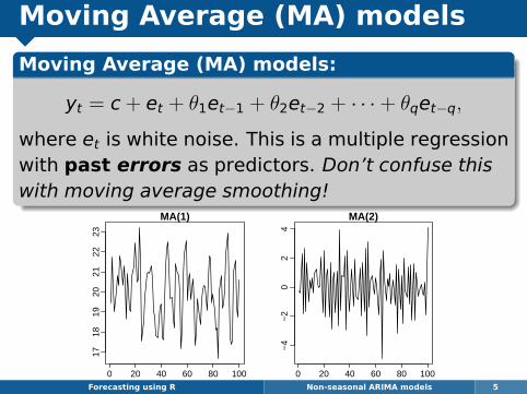
Moving Average (MA) models
Moving Average (MA) models:
yt = c+ et + θ1et−1 + θ2et−2 + · · ·+ θqet−q,
where et is white noise. This is a multiple regressionwith past errors as predictors. Don’t confuse thiswith moving average smoothing!
Forecasting using R Non-seasonal ARIMA models 5
Moving Average (MA) models
Moving Average (MA) models:
yt = c+ et + θ1et−1 + θ2et−2 + · · ·+ θqet−q,
where et is white noise. This is a multiple regressionwith past errors as predictors. Don’t confuse thiswith moving average smoothing!
MA(1)
Time
0 20 40 60 80 100
1718
1920
2122
23
MA(2)
Time
0 20 40 60 80 100
−4
−2
02
4
Forecasting using R Non-seasonal ARIMA models 5
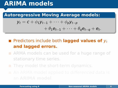
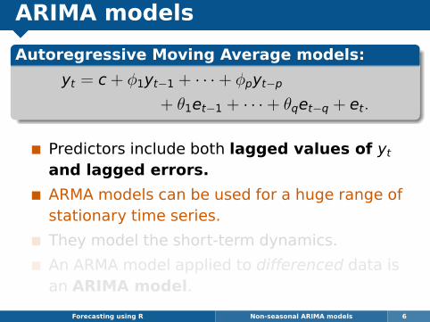
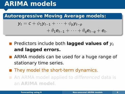
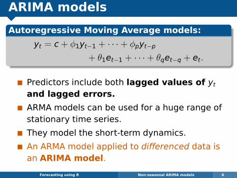
ARIMA models
Autoregressive Moving Average models:
yt = c+ φ1yt−1 + · · ·+ φpyt−p+ θ1et−1 + · · ·+ θqet−q + et.
Predictors include both lagged values of ytand lagged errors.
ARMA models can be used for a huge range ofstationary time series.
They model the short-term dynamics.
An ARMA model applied to differenced data isan ARIMA model.
Forecasting using R Non-seasonal ARIMA models 6
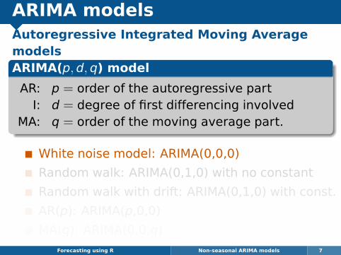
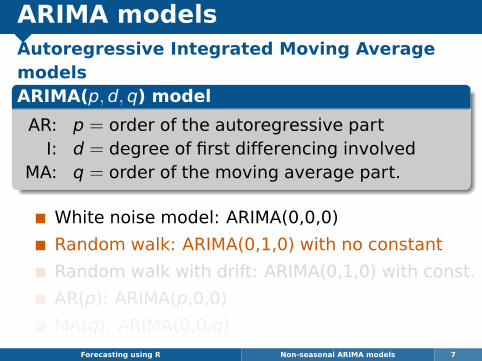
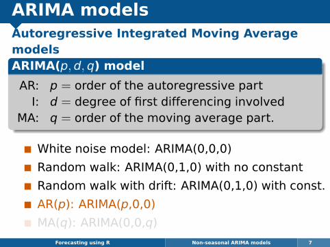
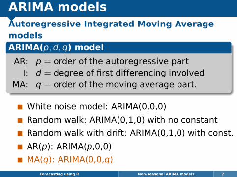
ARIMA modelsAutoregressive Integrated Moving AveragemodelsARIMA(p,d,q) model
AR: p = order of the autoregressive partI: d = degree of first differencing involved
MA: q = order of the moving average part.
White noise model: ARIMA(0,0,0)
Random walk: ARIMA(0,1,0) with no constant
Random walk with drift: ARIMA(0,1,0) with const.
AR(p): ARIMA(p,0,0)
MA(q): ARIMA(0,0,q)
Forecasting using R Non-seasonal ARIMA models 7
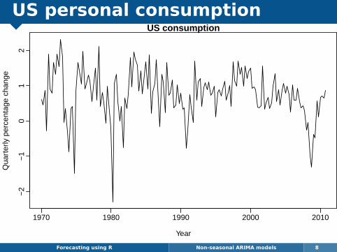
US personal consumption
Forecasting using R Non-seasonal ARIMA models 8
US consumption
Year
Qua
rter
ly p
erce
ntag
e ch
ange
1970 1980 1990 2000 2010
−2
−1
01
2
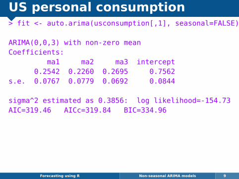
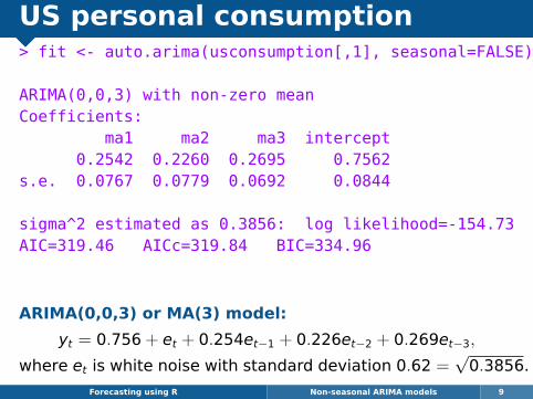
US personal consumption> fit <- auto.arima(usconsumption[,1], seasonal=FALSE)
ARIMA(0,0,3) with non-zero meanCoefficients:
ma1 ma2 ma3 intercept0.2542 0.2260 0.2695 0.7562
s.e. 0.0767 0.0779 0.0692 0.0844
sigma^2 estimated as 0.3856: log likelihood=-154.73AIC=319.46 AICc=319.84 BIC=334.96
Forecasting using R Non-seasonal ARIMA models 9
US personal consumption> fit <- auto.arima(usconsumption[,1], seasonal=FALSE)
ARIMA(0,0,3) with non-zero meanCoefficients:
ma1 ma2 ma3 intercept0.2542 0.2260 0.2695 0.7562
s.e. 0.0767 0.0779 0.0692 0.0844
sigma^2 estimated as 0.3856: log likelihood=-154.73AIC=319.46 AICc=319.84 BIC=334.96
ARIMA(0,0,3) or MA(3) model:
yt = 0.756 + et + 0.254et−1 + 0.226et−2 + 0.269et−3,
where et is white noise with standard deviation 0.62 =√
0.3856.
Forecasting using R Non-seasonal ARIMA models 9
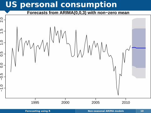
US personal consumption
Forecasting using R Non-seasonal ARIMA models 10
Forecasts from ARIMA(0,0,3) with non−zero mean
1995 2000 2005 2010
−1.
0−
0.5
0.0
0.5
1.0
1.5
2.0
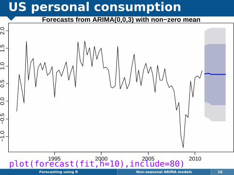
US personal consumption
Forecasting using R Non-seasonal ARIMA models 10
Forecasts from ARIMA(0,0,3) with non−zero mean
1995 2000 2005 2010
−1.
0−
0.5
0.0
0.5
1.0
1.5
2.0
plot(forecast(fit,h=10),include=80)
Understanding ARIMA models
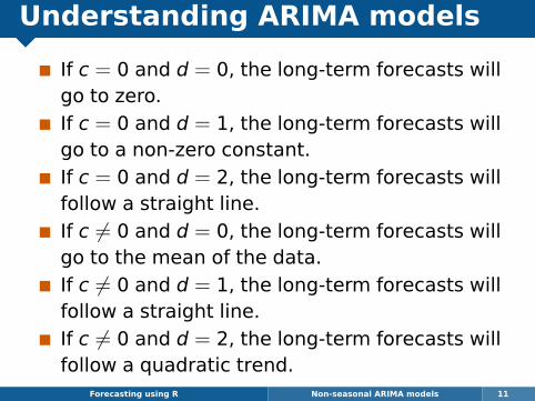
If c = 0 and d = 0, the long-term forecasts willgo to zero.If c = 0 and d = 1, the long-term forecasts willgo to a non-zero constant.If c = 0 and d = 2, the long-term forecasts willfollow a straight line.If c 6= 0 and d = 0, the long-term forecasts willgo to the mean of the data.If c 6= 0 and d = 1, the long-term forecasts willfollow a straight line.If c 6= 0 and d = 2, the long-term forecasts willfollow a quadratic trend.
Forecasting using R Non-seasonal ARIMA models 11
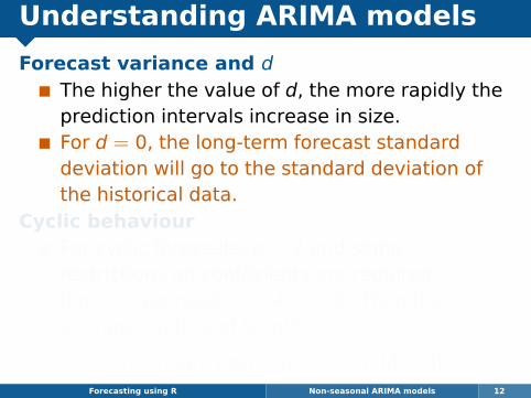
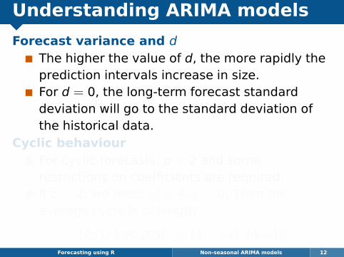
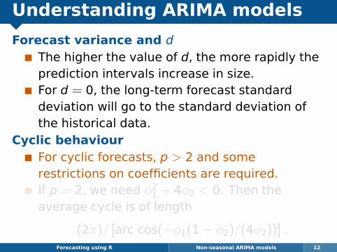
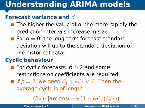
Understanding ARIMA models
Forecast variance and dThe higher the value of d, the more rapidly theprediction intervals increase in size.For d = 0, the long-term forecast standarddeviation will go to the standard deviation ofthe historical data.
Cyclic behaviourFor cyclic forecasts, p > 2 and somerestrictions on coefficients are required.If p = 2, we need φ2
1 + 4φ2 < 0. Then theaverage cycle is of length
(2π)/ [arc cos(−φ1(1− φ2)/(4φ2))] .Forecasting using R Non-seasonal ARIMA models 12
Outline
1 Non-seasonal ARIMA models
2 Estimation and order selection
3 ARIMA modelling in R
Forecasting using R Estimation and order selection 13
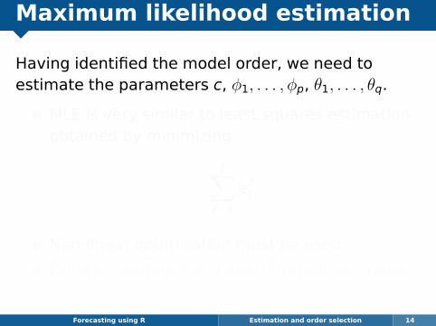
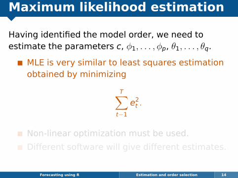
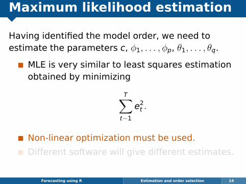
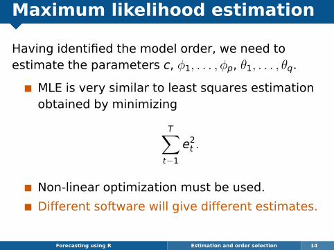
Maximum likelihood estimation
Having identified the model order, we need toestimate the parameters c, φ1, . . . , φp, θ1, . . . , θq.
MLE is very similar to least squares estimationobtained by minimizing
T∑t−1
e2t .
Non-linear optimization must be used.
Different software will give different estimates.
Forecasting using R Estimation and order selection 14
Outline
1 Non-seasonal ARIMA models
2 Estimation and order selection
3 ARIMA modelling in R
Forecasting using R ARIMA modelling in R 15
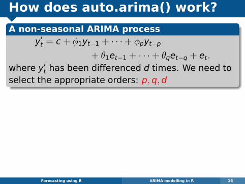
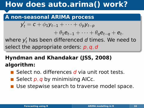
How does auto.arima() work?
A non-seasonal ARIMA processy′t = c+ φ1yt−1 + · · ·+ φpyt−p
+ θ1et−1 + · · ·+ θqet−q + et.where y′t has been differenced d times. We need toselect the appropriate orders: p,q,d
Forecasting using R ARIMA modelling in R 16
How does auto.arima() work?
A non-seasonal ARIMA processy′t = c+ φ1yt−1 + · · ·+ φpyt−p
+ θ1et−1 + · · ·+ θqet−q + et.where y′t has been differenced d times. We need toselect the appropriate orders: p,q,d
Hyndman and Khandakar (JSS, 2008)algorithm:
Select no. differences d via unit root tests.Select p,q by minimising AICc.Use stepwise search to traverse model space.
Forecasting using R ARIMA modelling in R 16
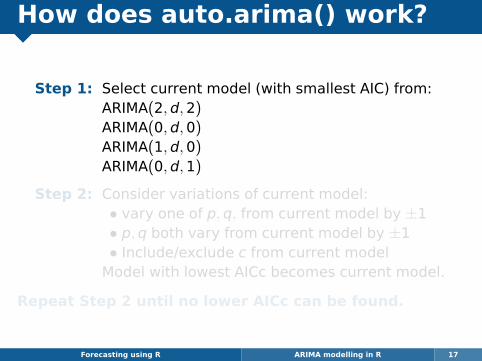
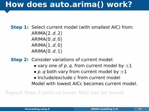
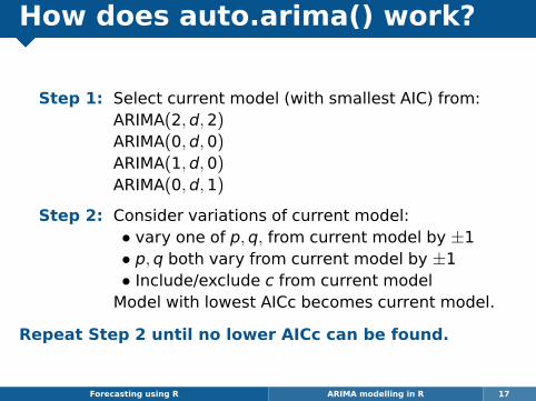
How does auto.arima() work?
Step 1: Select current model (with smallest AIC) from:ARIMA(2,d,2)ARIMA(0,d,0)ARIMA(1,d,0)ARIMA(0,d,1)
Step 2: Consider variations of current model:• vary one of p,q, from current model by ±1• p,q both vary from current model by ±1• Include/exclude c from current model
Model with lowest AICc becomes current model.
Repeat Step 2 until no lower AICc can be found.
Forecasting using R ARIMA modelling in R 17
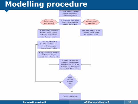
Modelling procedure
Forecasting using R ARIMA modelling in R 18
8/ arima models 177
1. Plot the data. Identifyunusual observations.Understand patterns.
2. If necessary, use a Box-Cox transformation tostabilize the variance.
Select modelorder yourself.
Use automatedalgorithm.
3. If necessary, differencethe data until it appearsstationary. Use unit-roottests if you are unsure.
4. Plot the ACF/PACF ofthe differenced data and
try to determine pos-sible candidate models.
5. Try your chosen model(s)and use the AICc to
search for a better model.
6. Check the residualsfrom your chosen model
by plotting the ACF of theresiduals, and doing a port-
manteau test of the residuals.
Use auto.arima() to findthe best ARIMA model
for your time series.
Do theresidualslook like
whitenoise?
7. Calculate forecasts.
yes
no
Figure 8.10: General process for fore-casting using an ARIMA model.
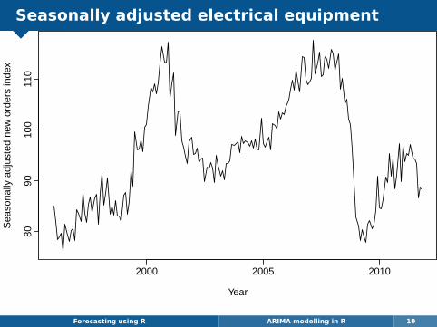
Seasonally adjusted electrical equipment
Forecasting using R ARIMA modelling in R 19
Year
Sea
sona
lly a
djus
ted
new
ord
ers
inde
x
2000 2005 2010
8090
100
110
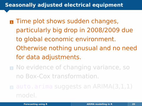
Seasonally adjusted electrical equipment
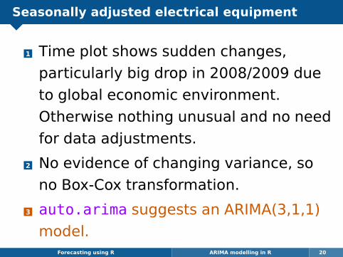
1 Time plot shows sudden changes,
particularly big drop in 2008/2009 due
to global economic environment.
Otherwise nothing unusual and no need
for data adjustments.
2 No evidence of changing variance, so
no Box-Cox transformation.
3 auto.arima suggests an ARIMA(3,1,1)
model.Forecasting using R ARIMA modelling in R 20
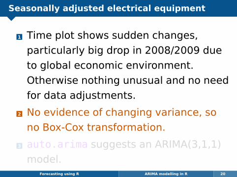
Seasonally adjusted electrical equipment
1 Time plot shows sudden changes,
particularly big drop in 2008/2009 due
to global economic environment.
Otherwise nothing unusual and no need
for data adjustments.
2 No evidence of changing variance, so
no Box-Cox transformation.
3 auto.arima suggests an ARIMA(3,1,1)
model.Forecasting using R ARIMA modelling in R 20
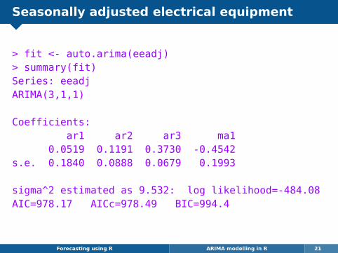
Seasonally adjusted electrical equipment
> fit <- auto.arima(eeadj)> summary(fit)Series: eeadjARIMA(3,1,1)
Coefficients:ar1 ar2 ar3 ma1
0.0519 0.1191 0.3730 -0.4542s.e. 0.1840 0.0888 0.0679 0.1993
sigma^2 estimated as 9.532: log likelihood=-484.08AIC=978.17 AICc=978.49 BIC=994.4
Forecasting using R ARIMA modelling in R 21
Seasonally adjusted electrical equipment
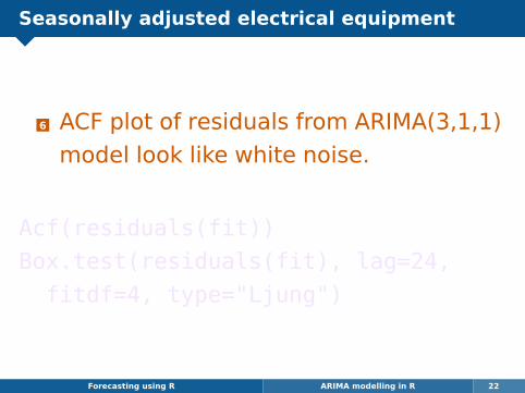
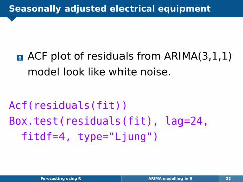
6 ACF plot of residuals from ARIMA(3,1,1)
model look like white noise.
Acf(residuals(fit))
Box.test(residuals(fit), lag=24,
fitdf=4, type="Ljung")
Forecasting using R ARIMA modelling in R 22
Seasonally adjusted electrical equipment
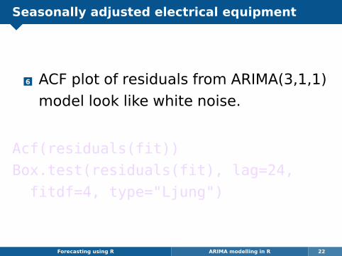
6 ACF plot of residuals from ARIMA(3,1,1)
model look like white noise.
Acf(residuals(fit))
Box.test(residuals(fit), lag=24,
fitdf=4, type="Ljung")
Forecasting using R ARIMA modelling in R 22
Seasonally adjusted electrical equipment
6 ACF plot of residuals from ARIMA(3,1,1)
model look like white noise.
Acf(residuals(fit))
Box.test(residuals(fit), lag=24,
fitdf=4, type="Ljung")
Forecasting using R ARIMA modelling in R 22
Seasonally adjusted electrical equipment
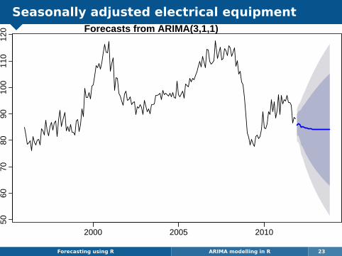
Forecasting using R ARIMA modelling in R 23
Forecasts from ARIMA(3,1,1)
2000 2005 2010
5060
7080
9010
011
012
0
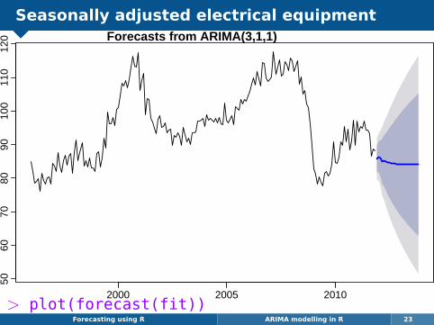
Seasonally adjusted electrical equipment
Forecasting using R ARIMA modelling in R 23
Forecasts from ARIMA(3,1,1)
2000 2005 2010
5060
7080
9010
011
012
0
> plot(forecast(fit))
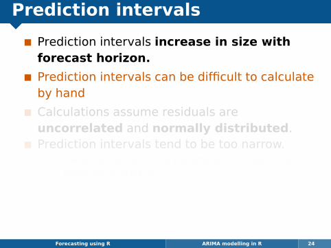
Prediction intervals
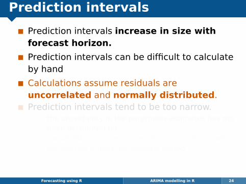
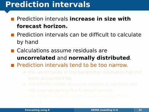
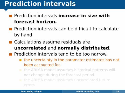
Prediction intervals increase in size withforecast horizon.
Prediction intervals can be difficult to calculateby hand
Calculations assume residuals areuncorrelated and normally distributed.Prediction intervals tend to be too narrow.
the uncertainty in the parameter estimates has notbeen accounted for.the ARIMA model assumes historical patterns willnot change during the forecast period.the ARIMA model assumes uncorrelated futureerrors
Forecasting using R ARIMA modelling in R 24
Prediction intervals
Prediction intervals increase in size withforecast horizon.
Prediction intervals can be difficult to calculateby hand
Calculations assume residuals areuncorrelated and normally distributed.Prediction intervals tend to be too narrow.
the uncertainty in the parameter estimates has notbeen accounted for.the ARIMA model assumes historical patterns willnot change during the forecast period.the ARIMA model assumes uncorrelated futureerrors
Forecasting using R ARIMA modelling in R 24