7. Digital Sine Oscillator Design 106 - · PDF file7. Digital Sine Oscillator Design 7.1...
21
7. Digital Sine Oscillator Design ________________________________________ 106 7.1 Overview ______________________________________________________________ 106 7.2 Recursive Oscillators ____________________________________________________ 107 7.2.1 The Biquad Oscillator ________________________________________________________ 107 7.2.2 The Coupled Form Oscillator __________________________________________________ 108 7.2.3 The Modified Coupled form Oscillator___________________________________________ 110 7.2.4 The Waveguide Oscillator_____________________________________________________ 111 7.2.5 Review of Recursive Oscillator Designs __________________________________________ 112 7.3 Phase-Accumulator Oscillators ____________________________________________ 113 7.4 Efficient Sine Calculation _________________________________________________ 114 7.4.1 Taylor’s Series______________________________________________________________ 114 7.4.2 Look-Up Tables_____________________________________________________________ 115 7.4.3 Linear Interpolated Look-Up Tables_____________________________________________ 116 7.4.4 Dither in Look-Up Tables _____________________________________________________ 118 7.4.5 Review ____________________________________________________________________ 118 7.5 CORDIC Vector Rotation Algorithm _______________________________________ 118 7.5.1 Definition _________________________________________________________________ 118 7.5.2 Application to Complex Oscillators _____________________________________________ 119 7.5.3 VLSI Implementation of CORDIC ______________________________________________ 121 7.5.4 Complex Oscillator Core with a CORDIC Pipeline _________________________________ 122 7.5.5 Determination of CORDIC S/N Performance from M and N__________________________ 123 7.6 Conclusions ____________________________________________________________ 125 Figure 7.1 The Biquad Oscillator______________________________________________________ 108 Figure 7.2 The Coupled form Oscillator ________________________________________________ 109 Figure 7.3 The Modified Coupled form Oscillator ________________________________________ 110 Figure 7.4 The Second Order Digital Waveguide Oscillator_________________________________ 112 Figure 7.5 The Phase-Accumulator Oscillator ___________________________________________ 113 Figure 7.6 Max Error (dB) of nth order Taylor’s Series approximation for sin(θ) ________________ 115 Figure 7.7 Pipeline Form of Interpolating LUT Oscillator __________________________________ 117 Figure 7.8 Dataflow for ith stage of CORDIC vector rotation _______________________________ 121 Figure 7.9 Schematic Diagram of CORDIC-based Complex Oscillator Core ___________________ 123 Figure 7.10 CORDIC Oscillator Performance____________________________________________ 124 Table 7-1 Summary of Recursive Oscillator Features ______________________________________ 113
-
Upload
duongthien -
Category
Documents
-
view
219 -
download
0
Transcript of 7. Digital Sine Oscillator Design 106 - · PDF file7. Digital Sine Oscillator Design 7.1...
7. Digital Sine Oscillator Design ________________________________________ 106
7.1 Overview ______________________________________________________________ 106
7.2 Recursive Oscillators ____________________________________________________ 107
7.2.1 The Biquad Oscillator________________________________________________________ 107
7.2.2 The Coupled Form Oscillator __________________________________________________ 108
7.2.3 The Modified Coupled form Oscillator___________________________________________ 110
7.2.4 The Waveguide Oscillator_____________________________________________________ 111
7.2.5 Review of Recursive Oscillator Designs __________________________________________ 112
7.3 Phase-Accumulator Oscillators ____________________________________________ 113
7.4 Efficient Sine Calculation _________________________________________________ 114
7.4.1 Taylor’s Series______________________________________________________________ 114
7.4.2 Look-Up Tables_____________________________________________________________ 115
7.4.3 Linear Interpolated Look-Up Tables_____________________________________________ 116
7.4.4 Dither in Look-Up Tables _____________________________________________________ 118
7.4.5 Review____________________________________________________________________ 118
7.5 CORDIC Vector Rotation Algorithm _______________________________________ 118
7.5.1 Definition _________________________________________________________________ 118
7.5.2 Application to Complex Oscillators _____________________________________________ 119
7.5.3 VLSI Implementation of CORDIC ______________________________________________ 121
7.5.4 Complex Oscillator Core with a CORDIC Pipeline _________________________________ 122
7.5.5 Determination of CORDIC S/N Performance from M and N__________________________ 123
7.6 Conclusions ____________________________________________________________ 125
Figure 7.1 The Biquad Oscillator______________________________________________________ 108
Figure 7.2 The Coupled form Oscillator ________________________________________________ 109
Figure 7.3 The Modified Coupled form Oscillator ________________________________________ 110
Figure 7.4 The Second Order Digital Waveguide Oscillator_________________________________ 112
Figure 7.5 The Phase-Accumulator Oscillator ___________________________________________ 113
Figure 7.6 Max Error (dB) of nth order Taylor’s Series approximation for sin(θ)________________ 115
Figure 7.7 Pipeline Form of Interpolating LUT Oscillator __________________________________ 117
Figure 7.8 Dataflow for ith stage of CORDIC vector rotation _______________________________ 121
Figure 7.9 Schematic Diagram of CORDIC-based Complex Oscillator Core ___________________ 123
Figure 7.10 CORDIC Oscillator Performance____________________________________________ 124
Table 7-1 Summary of Recursive Oscillator Features ______________________________________ 113
Page 106
7. Digital Sine Oscillator Design
7.1 Overview
Having determined a MAS paradigm with a variety of filterbank implementations, this
chapter is concerned with identifying efficient digital algorithms for the generation of
discrete-time sinusoids, with a bias towards their suitability for VLSI implementation, to
serve as the central core for the MAS Coprocessor (MASC) documented in Chapters 8
and 9. The topic of sinusoid generation is extensively researched and therefore the early
part of this chapter is a literature review. Both single-phase and complex algorithms (for
input into the PEF of section 5.3) are considered; the latter is an unusual application in a
digital audio context. For this reason, the latter part of the chapter (section 7.5) is
devoted to an analysis of a novel application of the CORDIC algorithm for AS / MAS.
Nonetheless, there are six desirable properties by which the different algorithms can be
assessed (the i subscript of Fi[n] etc. is omitted as a single prototype oscillator only is
under consideration):
• Low VLSI area.
• High throughput capacity to minimise the critical bottleneck of the TOB.
• A control rate for F[n] and A[n] at fs using PWL envelopes.
• Fine-resolution, linear response and wide dynamic range of F[n] and A[n].
• Non-interaction of A[n] and F[n]
• An output with a consistent S/N ratio independent of dynamic range.
There are two contrasting schools of sinusoidal oscillator design; (i) recursive and (ii)
phase-accumulator oscillators (Higgins, 1990). In general, recursive and phase-
accumulator approaches are associated respectively with software and hardware
implementations. Recursive oscillators, documented in section 7.1, are discrete-time
simulations of physical systems which have simple harmonic motion as their solution.
Cost of computation is dominated by the number of multiplies required per sample.
Page 107
Implementation in DSP’s is efficient because of the concentration of effort expended by
manufacturers in minimising multiplier delay . A disadvantage for AS is the difficulty of
dynamic frequency control at fs which is necessary for PWL enveloping. In contrast,
phase-accumulation as documented in section 7.3 presumes a control rate of fs. Indeed, it
is synonymous with the classical definition of AS in eqn. (1.1). The phase of the sinusoid
is computed explicitly from a discrete integration of F[n]. The main overhead is accurate
sine computation, historically obtained from LUT’s.
The choice depends on the context. An important design criterion is the ‘S/N’ ratio of
RMS signal and noise amplitudes: the difference between the approximate and idealised
output of a digital sine oscillator represents noise added to the signal which affects the
perceived purity of tone. The size of a direct LUT exponentiates with the required S/N
and hence if a high-fidelity stationary sinusoid is required, recursive designs are often
chosen. Also, as LUT size increases, so does propagation delay and a bottleneck forms in
the TOB as discussed in section 1.3.2. However, linear interpolation or CORDIC can
significantly accelerate throughput. Another strategy to reconcile the efficiency of
recursive oscillators with the controllability of phase-accumulation is to increase the
complexity of a recursive system such that it remains stable when the centre frequency is
updated at a rate of fs.
7.2 Recursive Oscillators
7.2.1 The Biquad Oscillator
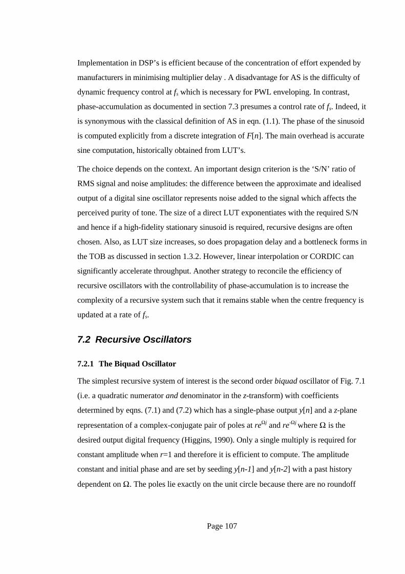
The simplest recursive system of interest is the second order biquad oscillator of Fig. 7.1
(i.e. a quadratic numerator and denominator in the z-transform) with coefficients
determined by eqns. (7.1) and (7.2) which has a single-phase output y[n] and a z-plane
representation of a complex-conjugate pair of poles at reΩj and re-Ωj where Ω is the
desired output digital frequency (Higgins, 1990). Only a single multiply is required for
constant amplitude when r=1 and therefore it is efficient to compute. The amplitude
constant and initial phase and are set by seeding y[n-1] and y[n-2] with a past history
dependent on Ω. The poles lie exactly on the unit circle because there are no roundoff
Page 108
errors for subtraction (b=-1) and thus the oscillator has excellent long term stability. The
set of available frequencies is linearly spaced and quantised by wordlength.
a r
b r
=
= −
22
cosΩ(7.1, 7.2)
Σ
z-1z-1
ab
y[n]
Figure 7.1 The Biquad Oscillator
A disadvantage for AS is that frequency and amplitude cannot be controlled dynamically
by changing the coefficients. Due to the second-order nature of the system, the past state
y[n-2] must be re-computed. In effect, a new segment of oscillation must be spliced into
the previous and so sample-rate resolution control is impractical. The oscillator is
constant amplitude and therefore imposition of amplitude requires an extra multiply on
y[n]. However, a second multiply enables b≠−1 and provides exponential growth (r>1)
or decay (0<r<1) which can be used for simulating primitive envelopes e.g. plucked
strings. The pole radius r represents inter-sample gain.
7.2.2 The Coupled Form Oscillator
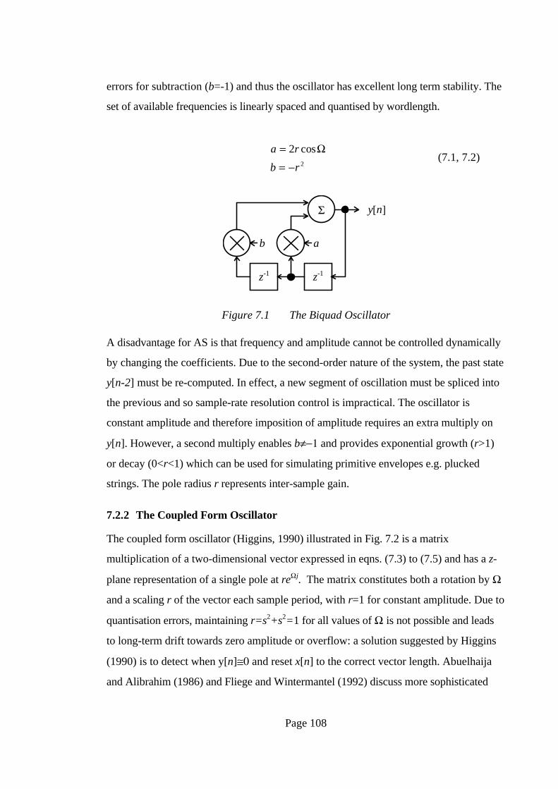
The coupled form oscillator (Higgins, 1990) illustrated in Fig. 7.2 is a matrix
multiplication of a two-dimensional vector expressed in eqns. (7.3) to (7.5) and has a z-
plane representation of a single pole at reΩj. The matrix constitutes both a rotation by Ω
and a scaling r of the vector each sample period, with r=1 for constant amplitude. Due to
quantisation errors, maintaining r=s2+s2=1 for all values of Ω is not possible and leads
to long-term drift towards zero amplitude or overflow: a solution suggested by Higgins
(1990) is to detect when y[n]≅0 and reset x[n] to the correct vector length. Abuelhaija
and Alibrahim (1986) and Fliege and Wintermantel (1992) discuss more sophisticated
Page 109
methods. Unlike the biquad oscillator, coefficients can be changed at the sample-rate
without the necessity to re-compute past states because the system is first order.
c r
s r
==
cos
sin
ΩΩ
(7.3, 7.4)
x n
y n
c s
s c
x n
y n
[ ])
[ ])
[ ]
[ ]
++
=
−
1
1(7.5)
Σ z-1+
s
x[n]
Σ z-1 y[n]
++
-
c c
Figure 7.2 The Coupled form Oscillator
The oscillator has a complex output but requires four multiplies per sample compared to
one for the biquad. However, it may execute at a sample rate equal to its output
bandwidth as explained in section 5.3.1; half that of a single-phase system like the
biquad. The output frequency range is therefore -π<Ω<π. Imposition of A[n] requires an
additional two multiplies on the output. An alternative is modulation of r (via s and c) at
a rate lower than fs for a piecewise exponential envelope relying on precision calculation
for accurate prediction of oscillator growth / decay over indefinite periods. However, as
discussed in section 1.1.3, PWL approximation is pre-eminent for modelling arbitrary
envelopes and its exponential alternative has minimal patronage.
For linear control of Ω via F[n], eqns. (7.3) and (7.4) must be computed every sample
period because of the non-linear relationship of s and c to F[n]. An alternative is to use
direct PWL approximations of the envelopes for s and c from F[n] such that eqns. (7.3)
and (7.4) require computation only at breakpoints. However, the interdependency of s
Page 110
and c in that c2+s2=r means that r will deviate from unity during PWL spans because of
the non-linearity, causing undesirable amplitude modulation. Also two envelopes are
used in place of one causing an increase in computation. Imposition of F[n] is thus
problematic for the coupled-form oscillator.
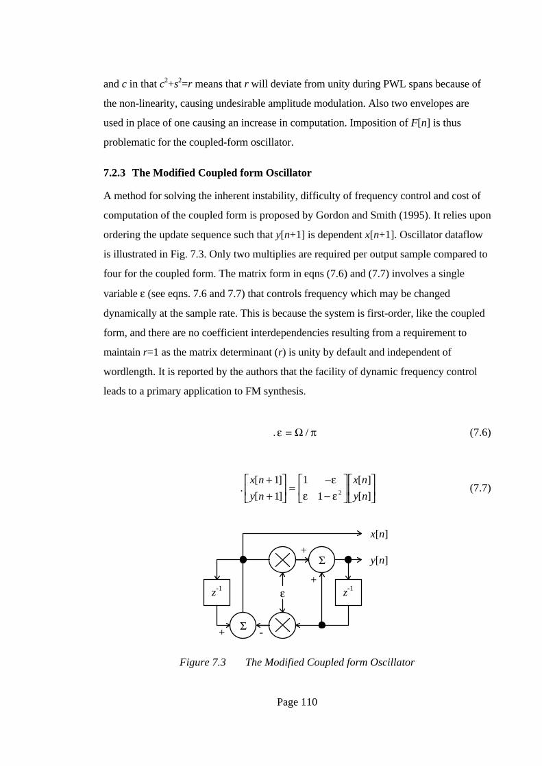
7.2.3 The Modified Coupled form Oscillator
A method for solving the inherent instability, difficulty of frequency control and cost of
computation of the coupled form is proposed by Gordon and Smith (1995). It relies upon
ordering the update sequence such that y[n+1] is dependent x[n+1]. Oscillator dataflow
is illustrated in Fig. 7.3. Only two multiplies are required per output sample compared to
four for the coupled form. The matrix form in eqns (7.6) and (7.7) involves a single
variable ε (see eqns. 7.6 and 7.7) that controls frequency which may be changed
dynamically at the sample rate. This is because the system is first-order, like the coupled
form, and there are no coefficient interdependencies resulting from a requirement to
maintain r=1 as the matrix determinant (r) is unity by default and independent of
wordlength. It is reported by the authors that the facility of dynamic frequency control
leads to a primary application to FM synthesis.
. ε π= Ω / (7.6)
.x n
y n
x n
y n
[ ]
[ ]
[ ]
[ ]
++
=
−−
1
1
1
1 2
εε ε
(7.7)
z-1
+
x[n]
Σ y[n]
+z-1
Σ+ -
ε
Figure 7.3 The Modified Coupled form Oscillator
Page 111
A strength of the modified coupled form for AS is that ε is a linear function of Ω (via
eqn. 7.6) in contrast to properties of the unmodified coupled form. An analysis of eqn.
(7.7) by the authors results in a prediction of (x[n], y[n]) given by eqns. (7.8) to (7.10)
which depends upon the initial condition of (x[0], y[0]). Setting (x[0], y[0])=(1, cos(ϕ))
results in (x[n], y[n])=(cos(nΩ), cos(nΩ-ϕ)) and conversely (x[0], y[0])=(1, -sin(ϕ))
results in (x[n], y[n])=(sin(nΩ), sin(nΩ-ϕ)). When Ω≅0, y[n] is in approximate
quadrature with x[n] since ϕ≅π/2 according to eqn. (7.8). However Ω≅±π results in ϕ≅0
and consequently, x[n] and y[n] are in approximate phase. Therefore the modified
coupled form is unsuitable for complex sinusoid generation which requires frequency-
independent quadrature between x[n] and y[n].
ϕ π= −( ) /Ω 2 (7.8)
G =+ −
− −
1
sin( )
sin( ) sin( )
sin( ) sin( )ϕϕ
ϕn n
n n
Ω ΩΩ Ω
(7.9)
x n
y n
x
yn[ ]
[ ]
[ ]
[ ]
=
G
0
0(7.10)
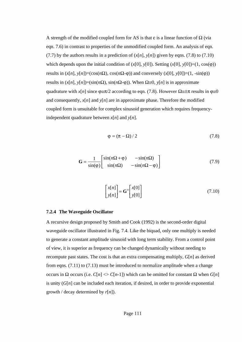
7.2.4 The Waveguide Oscillator
A recursive design proposed by Smith and Cook (1992) is the second-order digital
waveguide oscillator illustrated in Fig. 7.4. Like the biquad, only one multiply is needed
to generate a constant amplitude sinusoid with long term stability. From a control point
of view, it is superior as frequency can be changed dynamically without needing to
recompute past states. The cost is that an extra compensating multiply, G[n] as derived
from eqns. (7.11) to (7.13) must be introduced to normalize amplitude when a change
occurs in Ω occurs (i.e. C[n] <> C[n-1]) which can be omitted for constant Ω when G[n]
is unity (G[n] can be included each iteration, if desired, in order to provide exponential
growth / decay determined by r[n]).
Page 112
C n[ ] cos= Ω (7.11)
g n C n C n[ ] ( [ ]) ( [ ]= − +1 1 (7.12)
G n r n g n g n[ ] [ ] [ ] / [ ]= − 1 (7.13)
z-1
G[n]
Σ
+
Σ
Σ
z-1
C[n]
-
++
Figure 7.4 The Second Order Digital Waveguide Oscillator
The authors assert that such a scheme give the oscillator a controllability which is
suitable for FM synthesis at half the number of multiplies required for the modified
coupled form. It is also reported that AM as a by-product of FM when G[n] is unity has
acceptable side-effects upon timbre. Alternatively, a first order approximation of G[n] is
sufficient for amplitude normalisation. For the requirements of MAS, controllability is
not a significant improvement on the biquad oscillator. Like the modified coupled form,
the design is oriented towards an economic recursive implementation of FM synthesis.
7.2.5 Review of Recursive Oscillator Designs
Recursive oscillators have inherently poor controllabilty that improves with the
complexity of the design as summarised in Table 7.1. The coupled form is most
expensive and the only one suitable for use with a PEF filterbank. It suffers from stability
problems and non-linear frequency control, but as it has a complex quadrature output it
may execute at half the sample rate of single-phase oscillators. The biquad and
waveguide oscillators are cheapest to compute but have non-trivial frequency control
Page 113
problems at fs. The modified coupled-form therefore appears the best choice as it has a
single linear frequency control parameter and long-term stability. In all instances
imposition of the amplitude envelope A[n] from eqn (1.1) requires extra multiplies on the
output. All of the designs use two state variables as is to be expected of any second-
order system.
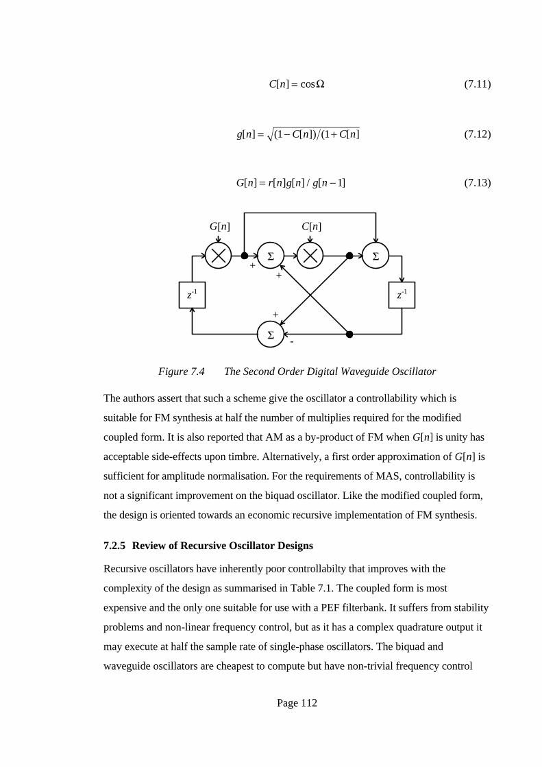
Design Multiplies per y[n] F[n] control Complex O/P
Biquad 2 inc A[n] Recompute history No
Coupled Form (CF) 6 ditto Non-linear, unstable Yes
Modified CF 3 ditto Linear, stable Not strictly
Waveguide 2 ditto Non-linear, stable No
Table 7-1 Summary of Recursive Oscillator Features
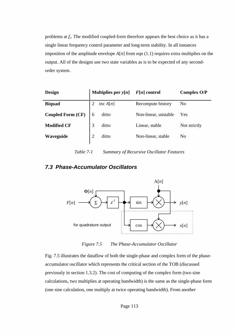
7.3 Phase-Accumulator Oscillators
sinΣ z-1 y[n]
cos x[n]
F[n]
Φ[n]
Α[n]
for quadrature output
Figure 7.5 The Phase-Accumulator Oscillator
Fig. 7.5 illustrates the dataflow of both the single-phase and complex form of the phase-
accumulator oscillator which represents the critical section of the TOB (discussed
previously in section 1.3.2). The cost of computing of the complex form (two sine
calculations, two multiplies at operating bandwidth) is the same as the single-phase form
(one sine calculation, one multiply at twice operating bandwidth). From another
Page 114
perspective, the former is more economic because the accumulation rate of Φ[n] is
halved as it is a part of the control domain where the rates of F[n] and A[n] are also
halved. For PWL envelopes, the number of interpolated envelope samples is therefore
halved but does not lead to a reduction in breakpoint bandwidth.
Two properties of phase accumulation are that (i) radians are an inconvenient unit for
binary arithmetic, and (ii) indefinite phase accumulation is unnecessary because sin(Φ[n])
is periodic. A classical solution (Moore, 1977) is to represent Φ[n] as a free-running
two’s complement accumulator with negative and positive full scale -fscale and fscale-1.
Multiplication of Φ[n] by (π/fscale) yields the true phase in radians, though this is
unnecessary in pre-normalised LUT addressing. Underflow or overflow of Φ[n]
implements modulo-2π accumulation. A requirement is that F[n] is pre-multiplied by
(π/fscale).
7.4 Efficient Sine Calculation
The efficiency of the phase-accumulator oscillator rests on the choice of algorithm for
computing sin(Φ[n]). Several options are reviewed in this section.
7.4.1 Taylor’s Series
sin( )! ! !
...( )( )!
(((! !
)!) )
θ θ θ θ θ θ π θ π
θ θ θ θ
= − + − + −−
≤ ≤
= − + − +
−−3 5 7
12 1
22 2
3 5 71
2 1 2
7
1
5
1
31
nn
n
n
where -2
for = 4
(7.13, 7.14)
The commonest numerical method for calculating sin(Φ[n]) is the Taylor’s series
expansion. It converges quickly to any required accuracy. The formula in eqn. (7.13) can
be factored using Horner’s algorithm to the form of eqn. (7.14) to optimise computation;
for n terms, n+1 multiplies, n-1 additions and n-1 constants are needed (Weltner et al,
1996). An extra multiply is required to denormalise Φ[n] or additional arithmetic to
implement true modulo-2π accumulation of Φ[n]. Only the first and fourth quadrants are
covered: the other two can be generated by a reflection.
Page 115
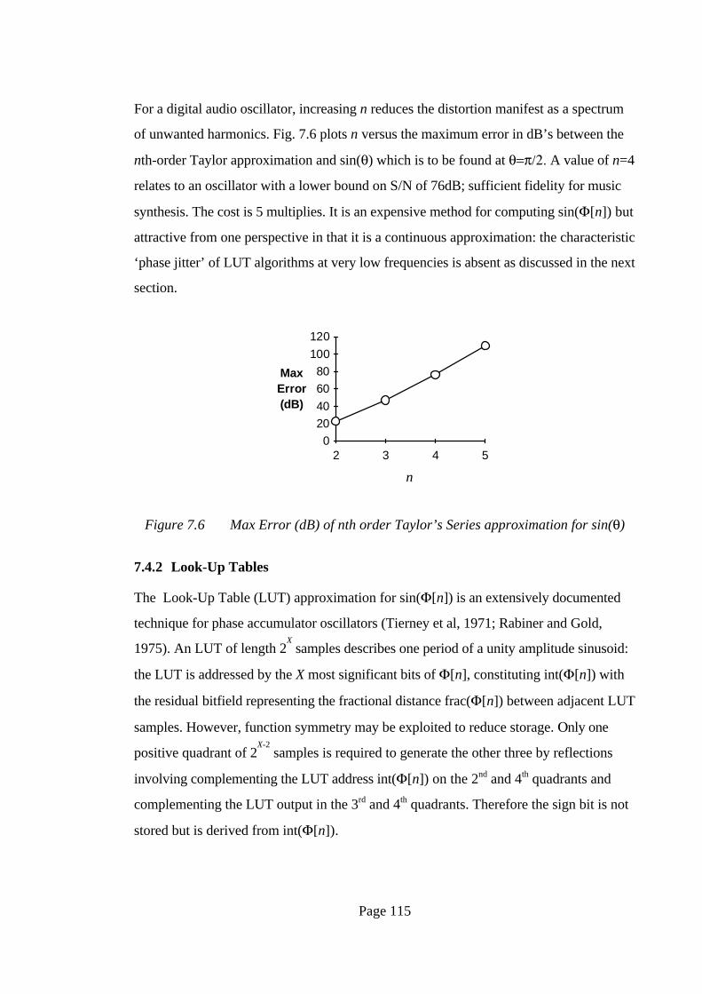
For a digital audio oscillator, increasing n reduces the distortion manifest as a spectrum
of unwanted harmonics. Fig. 7.6 plots n versus the maximum error in dB’s between the
nth-order Taylor approximation and sin(θ) which is to be found at θ=π/2. A value of n=4
relates to an oscillator with a lower bound on S/N of 76dB; sufficient fidelity for music
synthesis. The cost is 5 multiplies. It is an expensive method for computing sin(Φ[n]) but
attractive from one perspective in that it is a continuous approximation: the characteristic
‘phase jitter’ of LUT algorithms at very low frequencies is absent as discussed in the next
section.
n
MaxError(dB)
0
20
40
60
80
100
120
2 3 4 5
Figure 7.6 Max Error (dB) of nth order Taylor’s Series approximation for sin(θ)
7.4.2 Look-Up Tables
The Look-Up Table (LUT) approximation for sin(Φ[n]) is an extensively documented
technique for phase accumulator oscillators (Tierney et al, 1971; Rabiner and Gold,
1975). An LUT of length 2X samples describes one period of a unity amplitude sinusoid:
the LUT is addressed by the X most significant bits of Φ[n], constituting int(Φ[n]) with
the residual bitfield representing the fractional distance frac(Φ[n]) between adjacent LUT
samples. However, function symmetry may be exploited to reduce storage. Οnly one
positive quadrant of 2X-2
samples is required to generate the other three by reflections
involving complementing the LUT address int(Φ[n]) on the 2nd and 4th quadrants and
complementing the LUT output in the 3rd and 4th quadrants. Therefore the sign bit is not
stored but is derived from int(Φ[n]).
Page 116
Oscillator S/N is governed by two variables; (i) the number of samples 2X in a complete
cycle and, (ii) the stored sample wordlength N, excluding sign. The optimum
configuration (Moore, 1977) is N=X where worst-case S/N=6(X-2)dB. For a given value
of X, noise cannot be reduced by satisfying N>X because of phase quantisation
introduced by the effective discarding of frac(Φ[n]): commonly known as ‘phase jitter’
which has a quasi-harmonic spectrum. There are ways to reduce this. Rounding int(Φ[n])
on the basis of frac(Φ[n]) (i.e. to the nearest sample) improves S/N ratio by about 6dB
and requires an extra bit of resolution resulting in N=X+1 and S/N=6(X-1). Also “dither”
can be used to whiten the phase jitter spectrum (see section 7.4.4).
7.4.3 Linear Interpolated Look-Up Tables
An alternative to a fine resolution “direct” LUT is to use a coarser LUT with linear
interpolation between consecutive samples: high accuracy is possible as a single quadrant
of sin(Φ[n]) is a continuous function within finite bounds (Moore, 1977). The
computation has three stages:-
1. a=LUT[int(Φ[n])]
2. b=LUT[int(Φ[n])+1]-a.
3. sin(Φ[n])=a+b×frac(Φ[n])
The optimum configuration is N=2(X-1) where the worst-case S/N=12(X-1)dB. This
method approximately halves X but requires two LUT accesses, an addition, a
subtraction and a multiply step. It is attractive because, as X increases, savings in storage
requirements become considerable. For instance, for S/N>80dB, and storing a single
quadrant, a rounding oscillator has parameters X=15, N=16 constituting (16×215
)/4 =
16384 bytes whereas an equivalent interpolating oscillator has X=8, N=14 constituting
(14×28)/4 = 112 bytes. As the first quadrant of a sine is convex, the error caused by
interpolation always has a positive value. Adjusting each pair of points such that the
mean error over the corresponding interval is zero simply removes a DC offset and does
not alter the worst-case peak-to-peak error which determines worst-case S/N (Houghton
et al, 1995).
Page 117
There are two choices for VLSI implementation of an interpolated LUT oscillator; (i) a
single LUT can be accessed twice and b postcomputed, or (ii) two LUT’s in parallel
where the second LUT contains the precomputed b. Given the small LUT sizes, the
second option is more efficient because parallelism is exploited: such a solution is cited
by Snell (1977) and Chamberlin (1980). The multiply step frac(Φ[n])×b represents the
major overhead and, traditionally, an extra cycle of the Ai[n] multiplier implements this
but halves the throughput bandwidth of oscillator updates. However the maximum
wordlength required to represent b, upon analysis, is (N/2)+2, which is also the optimum
input wordlength for the interpolating multiplier and frac(Φ[n])): determined from
max(b)=2Nsin(2π/2X) when int(Φ[n])=0). For the specification S/N>80dB, a (14/2)+2=9-
bit ‘b’ LUT and multiplier is required for interpolation.
b
Σ
Φ[n]
sin(Φ[n])
integer
a
fraction Pipeline register -
Composite LUT
Inv
Inv
For 3rd and 4thQuadrants
For 2nd and 4thQuadrants
Inv
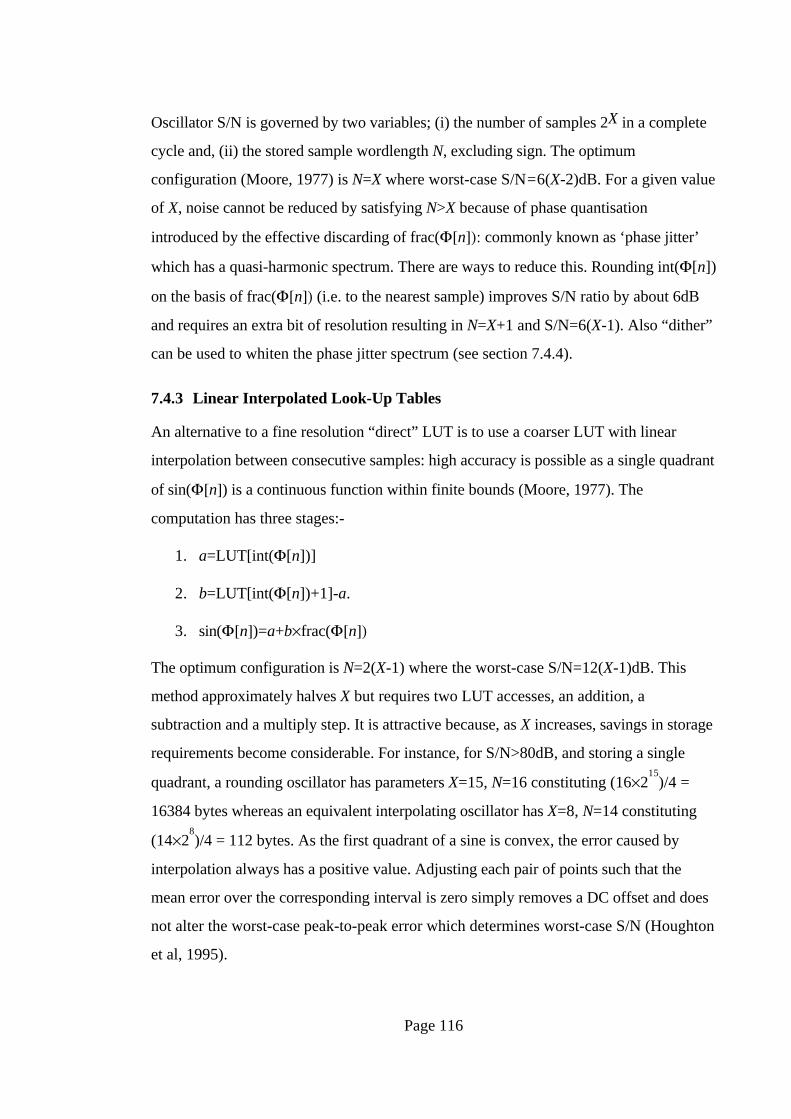
Figure 7.7 Pipeline Form of Interpolating LUT Oscillator
For VLSI implementation, a large rounding LUT presents two problems; (i) the silicon
area required for S/N>80dB (16 Kbytes) is large and (ii) the propogation delay of ROMs
increases with size posing the risk that it will determine an upper bound on TOB
throughput which cannot be increased by optimisations elsewhere in the TOB. Therefore
an interpolating oscillator appears to be a superior alternative. The option of two LUT’s,
one each for a and b, is fastest and may be pipelined with the subsequent multiplication /
accumulation step as illustrated in Fig. 7.7. As both LUT’s use the same address word -
int(Φ[n]) - extra efficiency is possible by coalescing both into a composite LUT. For
S/N>80dB, the composite LUT size is thus 64×(14+9) = 64×23 bits. The chief overhead
is the extra VLSI area required for the interpolation multiplier but since this quantity is
O(N2) (Weste and Eshraghian, 1988) the area in this case is only 92/162=32% of that
Page 118
envisaged for the 16-bit A[n] multiplier at the oscillator output. Such a structure is likely
to remove the critical bottleneck that computation of sin(Φ[n]) is perceived as forming in
a TOB (c.f. section 1.3.2).
7.4.4 Dither in Look-Up Tables
The idealised output spectrum of a digital sine oscillator is a single line at the desired
frequency with a flat noise floor determined by the output wordlength. In reality, the
output waveform of a practical LUT oscillator has a periodic quantisation noise
waveform superimposed upon it from a combination of phase-jitter and LUT truncation
error, which concentrates the noise power in a harmonic series of ‘spurs’ which can
produce perceptible overtones (Mehrgardt, 1983). A technique known as “dither” adds a
random signal in the range 0,1 to Φ[n], prior to truncation, in order to minimise noise
periodicity thus resulting in the desired flat noise (Flanagan and Zimmerman, 1993).
Houghton et al (1995) propose adding dither noise to the oscillator output.
7.4.5 Review
Computation of sin(Φ[n]) for AS is, therefore, most efficiently achieved by a
combination of table lookup and approximation, rather than an exclusive reliance on
either. A pipeline form of linear interpolation reduces the characteristic LUT bottleneck
in a TOB, as discussed in section 1.3.2, by exploiting parallelism. Such a configuration is
optimal for single-phase sinusoid generation. However, for a complex sinusoids,
inefficiency is manifest as a requirement to compute the quadrature component
cos(Φ[n]) by repeating the function computation with a modified argument cos(Φ[n])=
sin(Φ[n]-π/2) because the interdependency of sin(Φ[n]) and cos(Φ[n]) is not exploited.
7.5 CORDIC Vector Rotation Algorithm
7.5.1 Definition
The CORDIC (COordinate Rotation DIgital Computer) algorithm, reviewed by (Hu,
1992a), rotates a vector x+yj through an angle θ using M iterations of the set of eqns.
(7.15) to (7.18). The algorithm operates by constructing a successive approximation of
the rotation angle θ in terms of a unique set of weights αi∈+1,-1 for a summation
Page 119
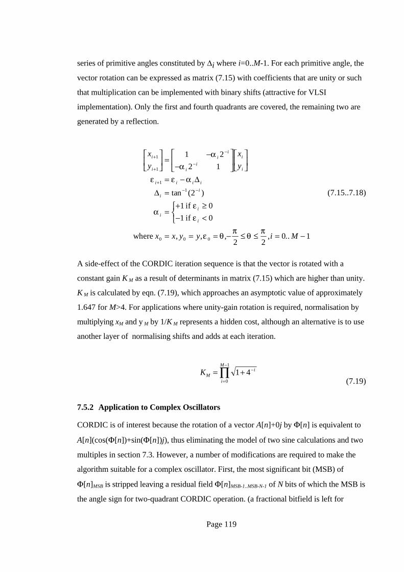
series of primitive angles constituted by ∆i where i=0..M-1. For each primitive angle, the
vector rotation can be expressed as matrix (7.15) with coefficients that are unity or such
that multiplication can be implemented with binary shifts (attractive for VLSI
implementation). Only the first and fourth quadrants are covered, the remaining two are
generated by a reflection.
x
y
x
y
x x y y i M
i
i
ii
ii
i
i
i i i i
ii
ii
i
+
+
−
−
+− −
=
−−
= −
=
=+ ≥− <
= = = − ≤ ≤ = −
1
1
1
1
0 0 0
1 2
2 1
2
1 0
1 0
2 20 1
αα
ε ε α
αεε
ε θ π θ π
∆
∆ tan ( )
, , , , ..
if
if
where
(7.15..7.18)
A side-effect of the CORDIC iteration sequence is that the vector is rotated with a
constant gain K M as a result of determinants in matrix (7.15) which are higher than unity.
K M is calculated by eqn. (7.19), which approaches an asymptotic value of approximately
1.647 for M>4. For applications where unity-gain rotation is required, normalisation by
multiplying xM and y M by 1/K M represents a hidden cost, although an alternative is to use
another layer of normalising shifts and adds at each iteration.
KMi
i
M
= + −
=
−
∏ 1 40
1
(7.19)
7.5.2 Application to Complex Oscillators
CORDIC is of interest because the rotation of a vector A[n]+0j by Φ[n] is equivalent to
A[n](cos(Φ[n])+sin(Φ[n])j), thus eliminating the model of two sine calculations and two
multiples in section 7.3. However, a number of modifications are required to make the
algorithm suitable for a complex oscillator. First, the most significant bit (MSB) of
Φ[n]MSB is stripped leaving a residual field Φ[n]MSB-1..MSB-N-1 of N bits of which the MSB is
the angle sign for two-quadrant CORDIC operation. (a fractional bitfield is left for
Page 120
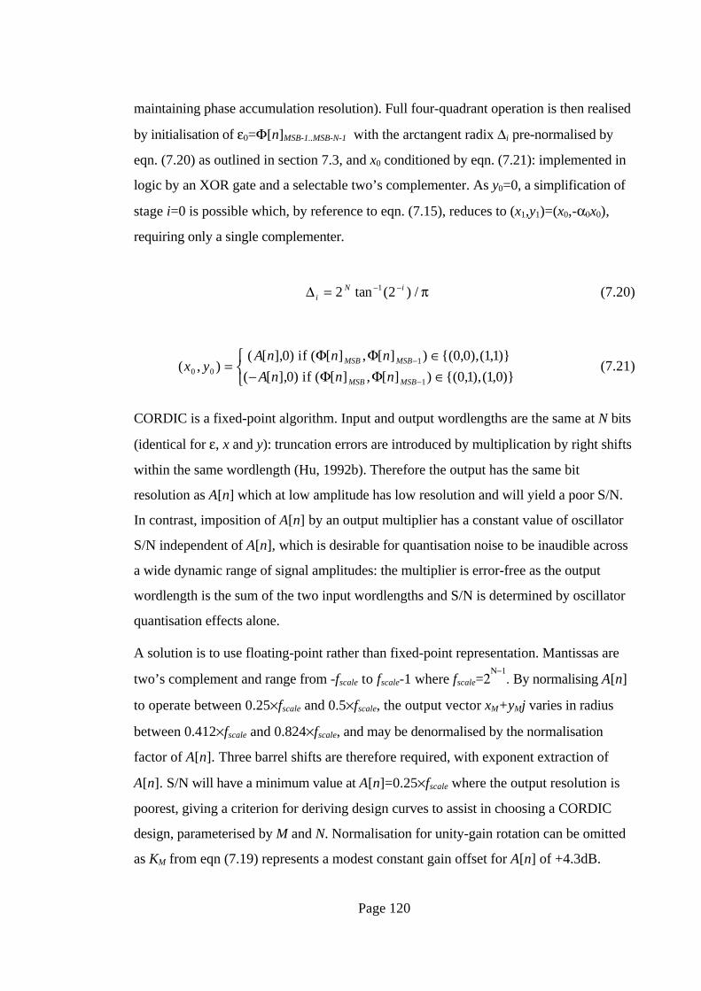
maintaining phase accumulation resolution). Full four-quadrant operation is then realised
by initialisation of ε0=Φ[n]MSB-1..MSB-N-1 with the arctangent radix ∆i pre-normalised by
eqn. (7.20) as outlined in section 7.3, and x0 conditioned by eqn. (7.21): implemented in
logic by an XOR gate and a selectable two’s complementer. As y0=0, a simplification of
stage i=0 is possible which, by reference to eqn. (7.15), reduces to (x1,y1)=(x0,-α0x0),
requiring only a single complementer.
∆ iN i= − −2 21tan ( ) / π (7.20)
( , )( [ ], ) [ ] , [ ] ) ( , ),( , )
( [ ], ) [ ] , [ ] ) ( , ),( , )x y
A n n n
A n n nMSB MSB
MSB MSB0 0
1
1
0 0 0 11
0 0 1 1 0=
∈− ∈
−
−
if (
if (
Φ ΦΦ Φ
(7.21)
CORDIC is a fixed-point algorithm. Input and output wordlengths are the same at N bits
(identical for ε, x and y): truncation errors are introduced by multiplication by right shifts
within the same wordlength (Hu, 1992b). Therefore the output has the same bit
resolution as A[n] which at low amplitude has low resolution and will yield a poor S/N.
In contrast, imposition of A[n] by an output multiplier has a constant value of oscillator
S/N independent of A[n], which is desirable for quantisation noise to be inaudible across
a wide dynamic range of signal amplitudes: the multiplier is error-free as the output
wordlength is the sum of the two input wordlengths and S/N is determined by oscillator
quantisation effects alone.
A solution is to use floating-point rather than fixed-point representation. Mantissas are
two’s complement and range from -fscale to fscale-1 where fscale=2Ν−1
. By normalising A[n]
to operate between 0.25×fscale and 0.5×fscale, the output vector xM+yMj varies in radius
between 0.412×fscale and 0.824×fscale, and may be denormalised by the normalisation
factor of A[n]. Three barrel shifts are therefore required, with exponent extraction of
A[n]. S/N will have a minimum value at A[n]=0.25×fscale where the output resolution is
poorest, giving a criterion for deriving design curves to assist in choosing a CORDIC
design, parameterised by M and N. Normalisation for unity-gain rotation can be omitted
as KM from eqn (7.19) represents a modest constant gain offset for A[n] of +4.3dB.
Page 121
7.5.3 VLSI Implementation of CORDIC
εi+1
2-i
/(+),(-)
Σ
/(+),(-)
Σ
/(+),(-)
Σ
xi+1
yi+1
∆i
εi
xi
yi
αi=sign(εi)
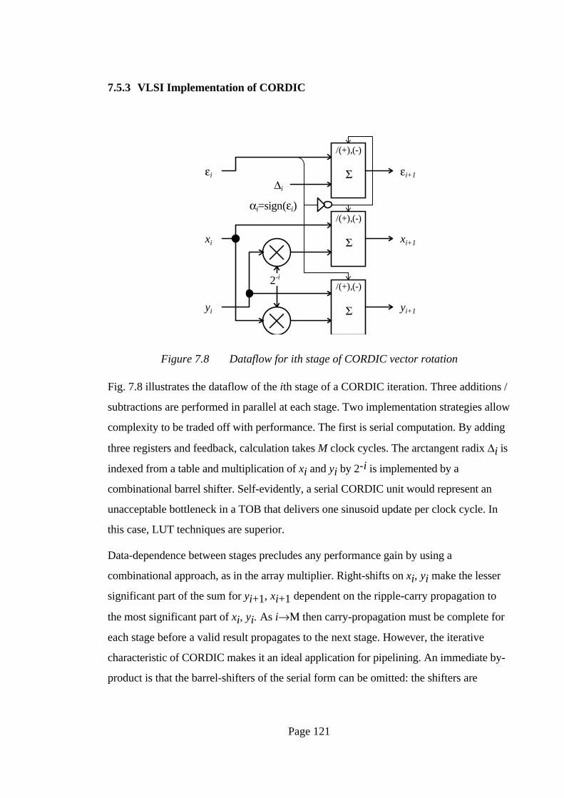
Figure 7.8 Dataflow for ith stage of CORDIC vector rotation
Fig. 7.8 illustrates the dataflow of the ith stage of a CORDIC iteration. Three additions /
subtractions are performed in parallel at each stage. Two implementation strategies allow
complexity to be traded off with performance. The first is serial computation. By adding
three registers and feedback, calculation takes M clock cycles. The arctangent radix ∆i is
indexed from a table and multiplication of xi and yi by 2-i is implemented by a
combinational barrel shifter. Self-evidently, a serial CORDIC unit would represent an
unacceptable bottleneck in a TOB that delivers one sinusoid update per clock cycle. In
this case, LUT techniques are superior.
Data-dependence between stages precludes any performance gain by using a
combinational approach, as in the array multiplier. Right-shifts on xi, yi make the lesser
significant part of the sum for yi+1, xi+1 dependent on the ripple-carry propagation to
the most significant part of xi, yi. As i→Μ then carry-propagation must be complete for
each stage before a valid result propagates to the next stage. However, the iterative
characteristic of CORDIC makes it an ideal application for pipelining. An immediate by-
product is that the barrel-shifters of the serial form can be omitted: the shifters are
Page 122
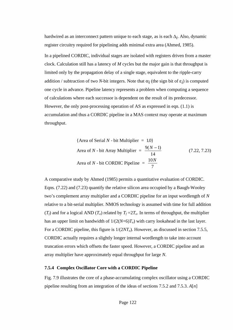
hardwired as an interconnect pattern unique to each stage, as is each ∆i. Also, dynamic
register circuitry required for pipelining adds minimal extra area (Ahmed, 1985).
In a pipelined CORDIC, individual stages are isolated with registers driven from a master
clock. Calculation still has a latency of M cycles but the major gain is that throughput is
limited only by the propagation delay of a single stage, equivalent to the ripple-carry
addition / subtraction of two N-bit integers. Note that αi (the sign bit of εi) is computed
one cycle in advance. Pipeline latency represents a problem when computing a sequence
of calculations where each successor is dependent on the result of its predecessor.
However, the only post-processing operation of AS as expressed in eqn. (1.1) is
accumulation and thus a CORDIC pipeline in a MAS context may operate at maximum
throughput.
Area of Serial - bit Multiplier =
Area of - bit Array Multiplier =
Area of - bit CORDIC Pipeline =
N
NN
NN
10
9 1
1410
7
.
( )−(7.22, 7.23)
A comparative study by Ahmed (1985) permits a quantitative evaluation of CORDIC.
Eqns. (7.22) and (7.23) quantify the relative silicon area occupied by a Baugh-Wooley
two’s complement array multiplier and a CORDIC pipeline for an input wordlength of N
relative to a bit-serial multiplier. NMOS technology is assumed with time for full addition
(Tf) and for a logical AND (Ta) related by Tf =2Ta. In terms of throughput, the multiplier
has an upper limit on bandwidth of 1/(2(N+6)Ta) with carry lookahead in the last layer.
For a CORDIC pipeline, this figure is 1/(2NTa). However, as discussed in section 7.5.5,
CORDIC actually requires a slightly longer internal wordlength to take into account
truncation errors which offsets the faster speed. However, a CORDIC pipeline and an
array multiplier have approximately equal throughput for large N.
7.5.4 Complex Oscillator Core with a CORDIC Pipeline
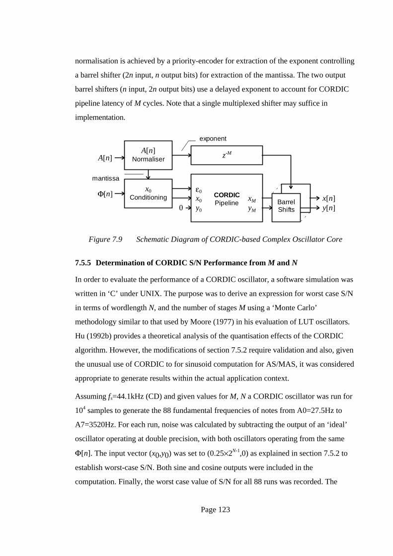
Fig. 7.9 illustrates the core of a phase-accumulating complex oscillator using a CORDIC
pipeline resulting from an integration of the ideas of sections 7.5.2 and 7.5.3. A[n]
Page 123
normalisation is achieved by a priority-encoder for extraction of the exponent controlling
a barrel shifter (2n input, n output bits) for extraction of the mantissa. The two output
barrel shifters (n input, 2n output bits) use a delayed exponent to account for CORDIC
pipeline latency of M cycles. Note that a single multiplexed shifter may suffice in
implementation.
A[n]Normaliser
x0Conditioning CORDIC
Pipeline
z-M
ε0
x0
y0
xM
yM
exponent
mantissa
0BarrelShifts
x[n]y[n]
A[n]
Φ[n]
Figure 7.9 Schematic Diagram of CORDIC-based Complex Oscillator Core
7.5.5 Determination of CORDIC S/N Performance from M and N
In order to evaluate the performance of a CORDIC oscillator, a software simulation was
written in ‘C’ under UNIX. The purpose was to derive an expression for worst case S/N
in terms of wordlength N, and the number of stages M using a ‘Monte Carlo’
methodology similar to that used by Moore (1977) in his evaluation of LUT oscillators.
Hu (1992b) provides a theoretical analysis of the quantisation effects of the CORDIC
algorithm. However, the modifications of section 7.5.2 require validation and also, given
the unusual use of CORDIC to for sinusoid computation for AS/MAS, it was considered
appropriate to generate results within the actual application context.
Assuming fs=44.1kHz (CD) and given values for M, N a CORDIC oscillator was run for
104 samples to generate the 88 fundamental frequencies of notes from A0=27.5Hz to
A7=3520Hz. For each run, noise was calculated by subtracting the output of an ‘ideal’
oscillator operating at double precision, with both oscillators operating from the same
Φ[n]. The input vector (x0,y0) was set to (0.25×2N-1,0) as explained in section 7.5.2 to
establish worst-case S/N. Both sine and cosine outputs were included in the
computation. Finally, the worst case value of S/N for all 88 runs was recorded. The
Page 124
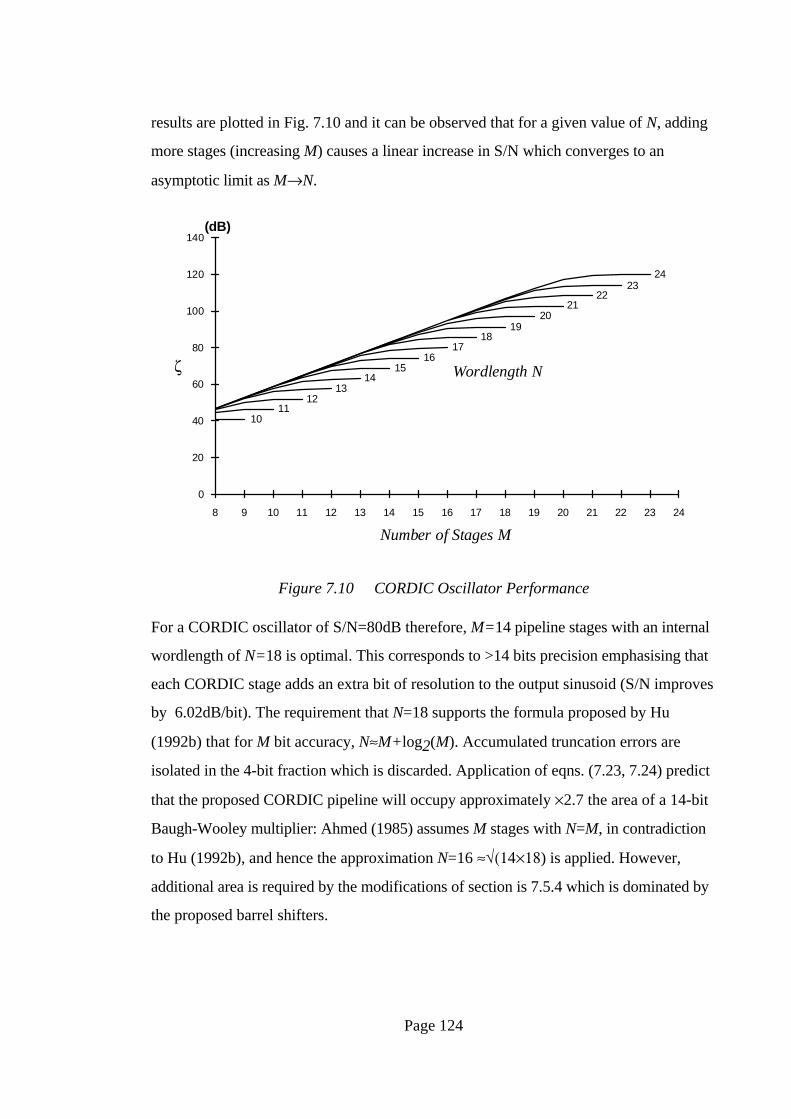
results are plotted in Fig. 7.10 and it can be observed that for a given value of N, adding
more stages (increasing M) causes a linear increase in S/N which converges to an
asymptotic limit as M→N.
Number of Stages M
ζ
0
20
40
60
80
100
120
140
8 9 10 11 12 13 14 15 16 17 18 19 20 21 22 23 24
Wordlength N
1011
1213
1415
1617
1819
2021
2223
24
(dB)
Figure 7.10 CORDIC Oscillator Performance
For a CORDIC oscillator of S/N=80dB therefore, M=14 pipeline stages with an internal
wordlength of N=18 is optimal. This corresponds to >14 bits precision emphasising that
each CORDIC stage adds an extra bit of resolution to the output sinusoid (S/N improves
by 6.02dB/bit). The requirement that N=18 supports the formula proposed by Hu
(1992b) that for M bit accuracy, N≈M+log2(M). Accumulated truncation errors are
isolated in the 4-bit fraction which is discarded. Application of eqns. (7.23, 7.24) predict
that the proposed CORDIC pipeline will occupy approximately ×2.7 the area of a 14-bit
Baugh-Wooley multiplier: Ahmed (1985) assumes M stages with N=M, in contradiction
to Hu (1992b), and hence the approximation N=16 ≈√(14×18) is applied. However,
additional area is required by the modifications of section is 7.5.4 which is dominated by
the proposed barrel shifters.
Page 125
7.6 Conclusions
From the survey, there are two efficient schemes for the realisation of a single-phase
oscillator bank which satisfy the requirements of section 7.1; (i) the modified coupled
form (recursive) and (ii) the pipelined linear-interpolated LUT (phase-accumulator). The
former requires three multiplies (including imposition of A[n]) per sample, uses two state
variables (x[n], y[n]) and phase is accumulated implicitly. The latter requires only a single
variable for explicit phase accumulation (Φ[n]) and a single multiply for A[n], with a
reduced wordlength multiply for interpolation and small LUT. Custom hardware is
required to exploit its efficiency, but in such a form is more economic than the modified
coupled form and hence is the recommended choice for VLSI implementation.
A complex oscillator bank for use with the PEF of section 3.7 is of similar computational
complexity to its single phase equivalent. A modified CORDIC algorithm offers an
alternative to two parallel instantiations of a pipelined linear-interpolated LUT. In spite
of comparable performance, the relative VLSI design complexities will favour the
simplicity of the latter approach as it is composed of a small set of standard components,
which will be highly optimised. However, formulation of the CORDIC digital sine
oscillator, hitherto uninvestigated for its application to AS, serves as an interesting
contrast to the other techniques.