6.02 Fall 2012 Lecture 16 Slide #1

6.02 Fall 2012 Lecture #16

•  DTFT vs DTFS •  Modulation/Demodulation •  Frequency Division Multiplexing

(FDM)

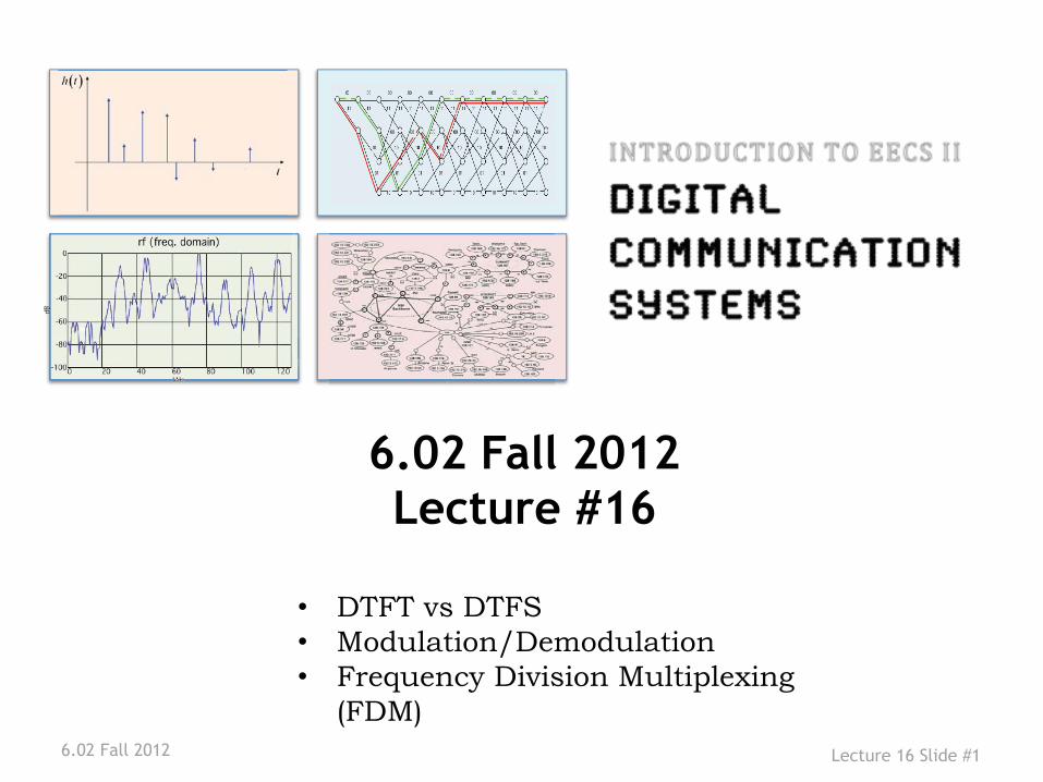
Fast Fourier Transform (FFT) to compute samples of the DTFT for signals of finite dura tion

P−1 1 X(Ωk ) = ∑ x[m]e− jΩkm, x[n] =

m=0 P

6.02 Fall 2012 Lecture 16 Slide #2

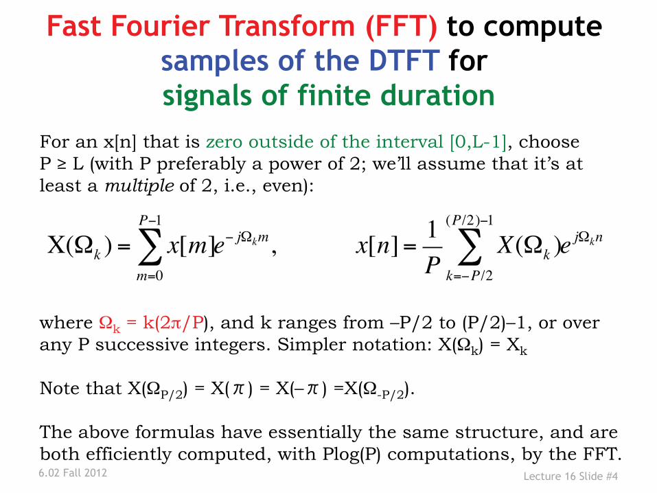
For an x[n] that is zero outside of the interval [0,L-1], choose P ≥ L (with P preferably a power of 2; we’ll assume that it’s at least a multiple of 2, i.e., even):

(P/2)−1

∑ X(Ωk )ejΩkn

k=−P/2

where Ωk = k(2π/P), and k ranges from –P/2 to (P/2)–1, or over any P successive integers. Simpler notation: X(Ωk) = Xk

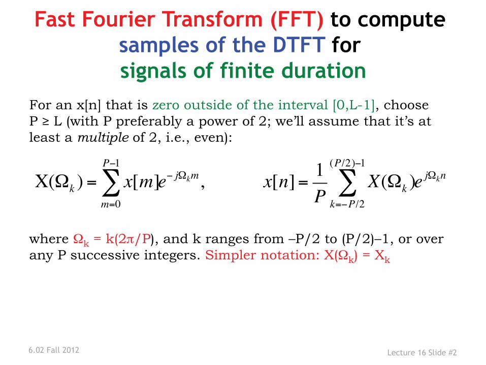
Where do the Ω

6.02 Fall 2012 Lecture 16 Slide #3

Ωk live? e.g., for P=6 (even )

– 0

Ω0� Ω1� Ω2� Ω3�Ω 3� Ω 2� Ω 1�

exp(jΩ0)�

exp(jΩ 1)�

exp(jΩ2)�

exp(jΩ3)�= exp(jΩ 3)

exp(jΩ1)�

exp(jΩ 2)�

. 1 –1

j

–j

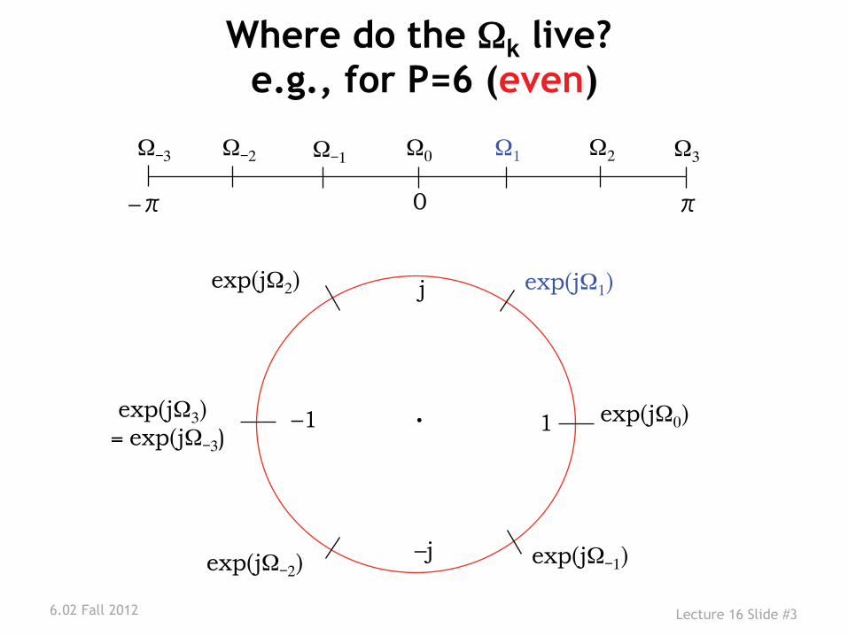
Fast Fourier Transform (FFT) to compute samples of the DTFT for signals of finite dura tion

P−1 1 X(Ωk ) = ∑ x[m]e− jΩkm, x[n] =

m=0 P

6.02 Fall 2012 Lecture 16 Slide #4

For an x[n] that is zero outside of the interval [0,L-1], choose P ≥ L (with P preferably a power of 2; we’ll assume that it’s at least a multiple of 2, i.e., even):

(P/2)−1

∑ X(Ωk )ejΩkn

k=−P/2

where Ωk = k(2π/P), and k ranges from –P/2 to (P/2)–1, or over any P successive integers. Simpler notation: X(Ωk) = Xk Note that X(Ω ) = X( ) = X(–P/2 ) =X(Ω-P/2). The above formulas have essentially the same structure, and are both efficiently computed, with Plog(P) computations, by the FFT.

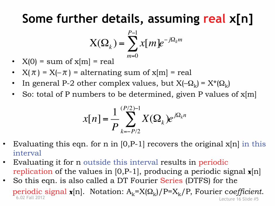
Some further details, assuming real x[n]P−1

X(Ω ) = ∑ x[m]e− jΩkmk

m=0•  X(0) = sum of x[m] = real

•  X( ) = X(– ) = alternating sum of x[m] = real •  In general P-2 other complex values, but X(–Ωk) = X*(Ωk)

•  So: total of P numbers to be determined, given P values of x[m]

1x[n] =

P

6.02 Fall 2012 Lecture 16 Slide #5

(P/2)−1

∑ X(Ωk )ejΩkn

k=−P/2

•  Evaluating this eqn. for n in [0,P-1] recovers the original x[n] in this interval

•  Evaluating it for n outside this interval results in periodic replication of the values in [0,P-1], producing a periodic signal x[n]

•  So this eqn. is also called a DT Fourier Series (DTFS) for the

periodic signal x[n]. Notation: Ak=X(Ωk)/P=Xk/P, Fourier coefficient.

Why the periodicity of x

6.02 Fall 2012 Lecture 16 Slide #6

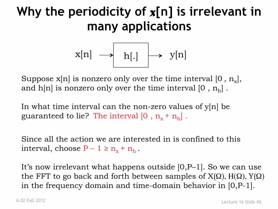
x[n] is irrelevant in many applications

h[.] x[n] y[n]

Suppose x[n] is nonzero only over the time interval [0 , nx], and h[n] is nonzero only over the time interval [0 , nh] . In what time interval can the non-zero values of y[n] be guaranteed to lie? The interval [0 , nx + nh] .

Since all the action we are interested in is confined to this interval, choose P – 1 ≥ nx + nh . It’s now irrelevant what happens outside [0,P–1]. So we can use the FFT to go back and forth between samples of X(Ω), Η(Ω), Y(Ω) �in the frequency domain and time-domain behavior in [0,P-1].

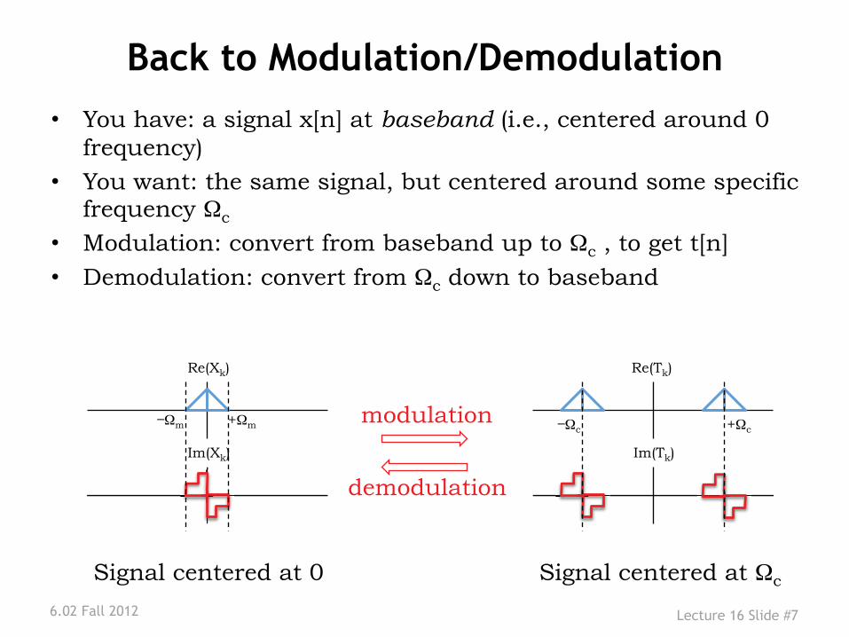
Back to Modulation/Demodulation •  You have: a signal x[n] at baseband (i.e., centered around 0

frequency)

•  You want: the same signal, but centered around some specific frequency Ωc

•  Modulation: convert from baseband up to Ωc , to get t[n] •  Demodulation: convert from Ωc down to baseband

6.02 Fall 2012 Lecture 16 Slide #7

Re(Xk)

Im(Xk)

+Ωm Ωm

Re(Tk)

Im(Tk)

+Ωc Ωc modulation

demodulation

Signal centered at 0 Signal centered at Ωc

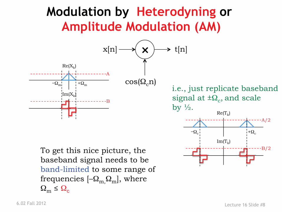
Modulation by Heterodyning or Amplitude Modulation (AM)

6.02 Fall 2012 Lecture 16 Slide #8

×x[n]

cos(Ωcn)

t[n]

Im(Tk)

+Ωc Ωc

B/2

k

A/2

Re(T )

i.e., just replicate baseband signal at ±Ωc, and scale by ½.

k

Im(Xk)

+Ωm Ωm

A

B

Re(X )

To get this nice picture, the baseband signal needs to be band-limited to some range of frequencies [–Ωm,Ωm], where Ωm ≤ Ωc

6.02 Fall 2012 Lecture 16 Slide #9

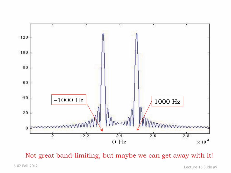
0 Hz

1000 Hz –1000 Hz

Not great band-limiting, but maybe we can get away with it!

At the Receiver: Demodulation•  In principle, this is (as easy as) modulation again:

If the received signal is r[n] = x[n]cos(Ωcn) = t[n],

(no distortion or noise) then simply compute

d[n] = r[n]cos(Ωcn)

= x[n]cos2(Ωcn)

= 0.5 {x[n] + x[n]cos(2Ωcn)} If there is distortion (i.e., r[n] ≠ t[n]), then write y[n] instead of

x[n] (and hope that in the noise-free case y[.] is related to x[.] by an approximately LTI relationship!)

•  What does the spectrum of d[n], i.e., D(Ω), look like?

•  What constraint on the bandwidth of x[n] is needed for perfect recovery of x[n]?

6.02 Fall 2012 Lecture 16 Slide #10

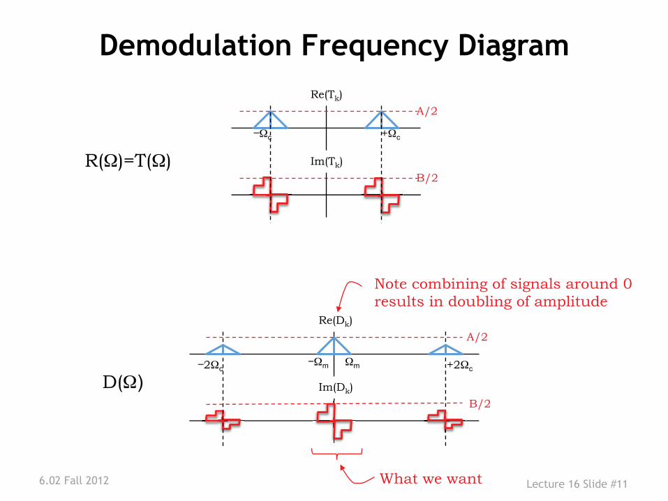
Demodulation Frequency Diagra m

6.02 Fall 2012 Lecture 16 Slide #11

Im(Tk)

+Ωc Ωc

A/2

B/2

kRe(T )

Im(Dk)

2Ωc

A/2

B/2

+2Ωc Ωm Ωm

Re(Dk)

R(Ω)=T(Ω)

D(Ω)

What we want

Note combining of signals around 0 results in doubling of amplitude

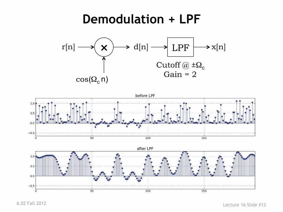
Demodulation + LPF

6.02 Fall 2012 Lecture 16 Slide #12

×r[n]

cos(Ωc n)

d[n] LPF x[n]

Cutoff @ ±Ωc Gain = 2

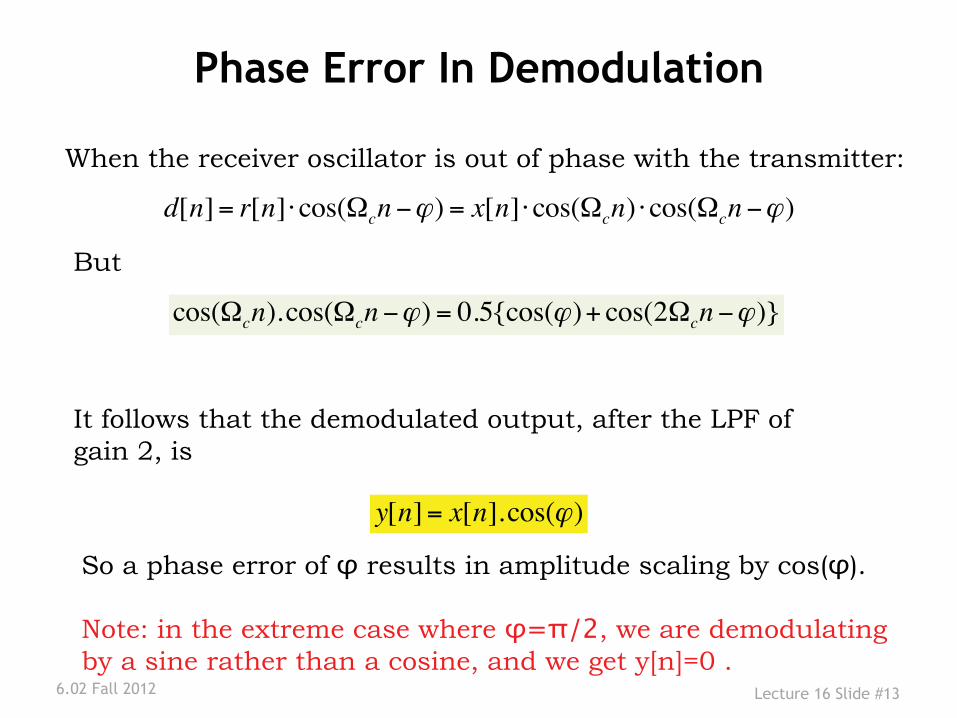
Phase Error In Demodulation

When the receiver oscillator is out of phase with the transmitter:

d[n] = r[n]⋅ cos(Ωcn−ϕ ) = x[n]⋅ cos(Ωcn) ⋅ cos(Ωcn−ϕ )

6.02 Fall 2012 Lecture 16 Slide #13

y[n] = x[n].cos(ϕ )

So a phase error of φ results in amplitude scaling by cos(φ). Note: in the extreme case where φ=�/2, we are demodulating by a sine rather than a cosine, and we get y[n]=0 .

But

cos(Ωcn).cos(Ωcn−ϕ ) = 0.5{cos(ϕ )+ cos(2Ωcn−ϕ )}

It follows that the demodulated output, after the LPF of gain 2, is

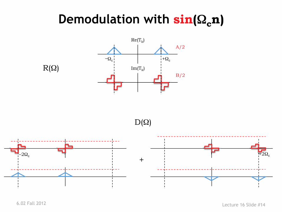
Demodulation with sin(Ω

6.02 Fall 2012 Lecture 16 Slide #14

Ωc n)

+ +2Ωc –2Ωc

D(Ω)

Im(Tk)

+Ωc Ωc

A/2

B/2

Re(Tk)

R(Ω)

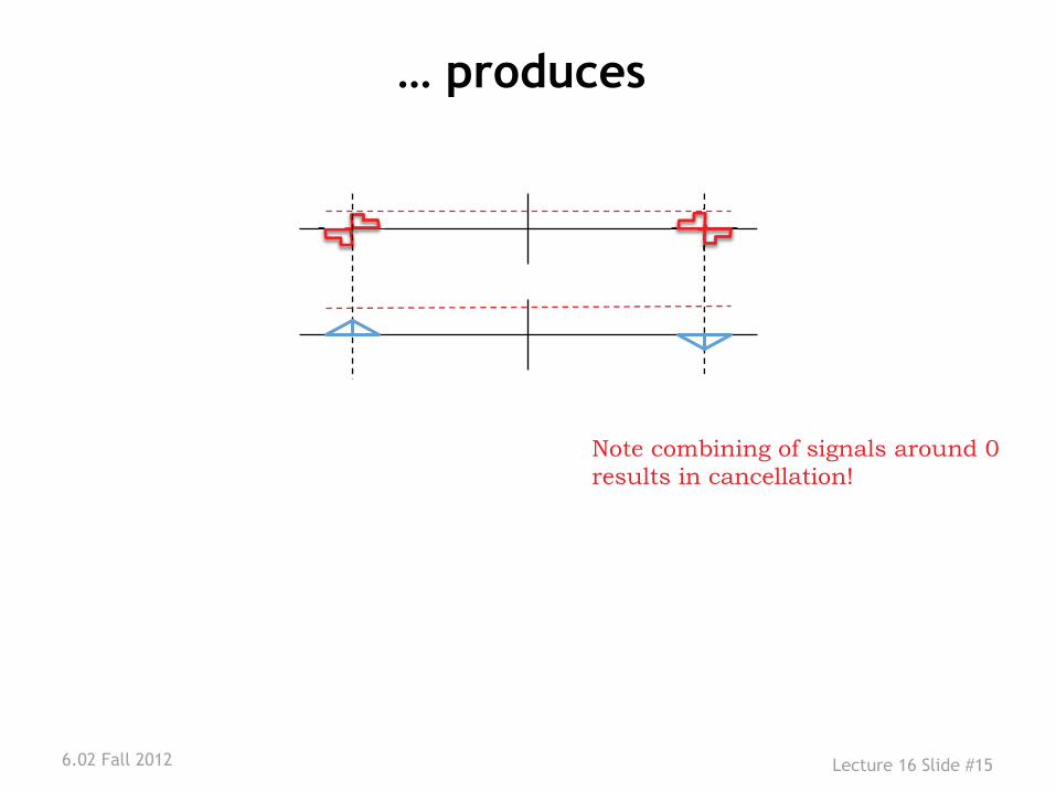
… produces

6.02 Fall 2012 Lecture 16 Slide #15

Note combining of signals around 0 results in cancellation!

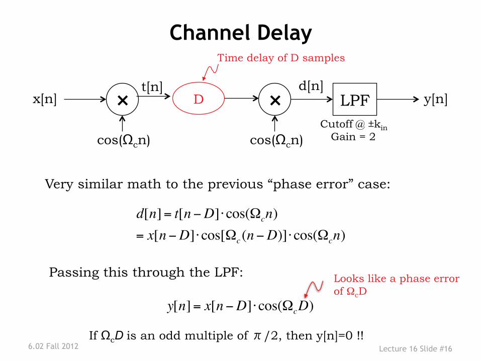
Channel Delay

6.02 Fall 2012 Lecture 16 Slide #16

×t[n] d[n]

LPF y[n]

Cutoff @ ±kin Gain = 2

×cos(Ωcn)

x[n] D

Time delay of D samples

d[n] = t[n−D]⋅ cos(Ωcn)

= x[n−D]⋅ cos[Ωc (n−D)]⋅ cos(Ωcn)

Passing this through the LPF: Looks like a phase error of ΩcD

y[n] = x[n−D]⋅ cos(ΩcD)D)

cos(Ωcn)

Very similar math to the previous “phase error” case:

If ΩcD is an odd multiple of /2, then y[n]=0 !!

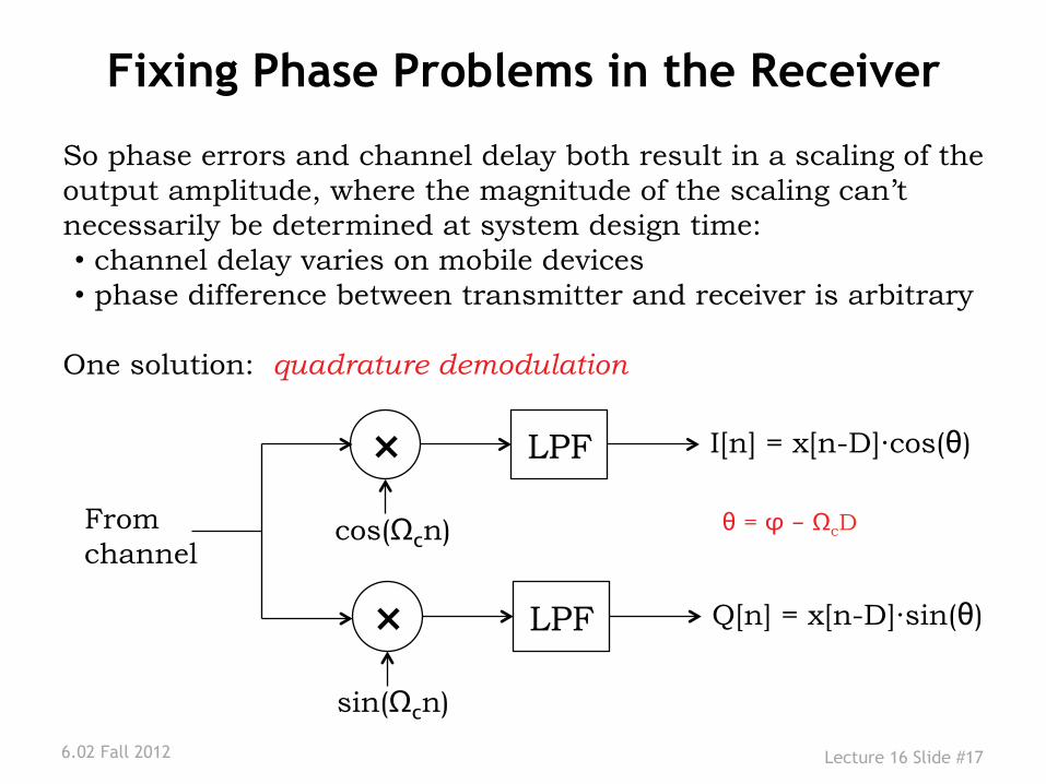
Fixing Phase Problems in the Receiver

So phase errors and channel delay both result in a scaling of the output amplitude, where the magnitude of the scaling can’t necessarily be determined at system design time: •  channel delay varies on mobile devices •  phase difference between transmitter and receiver is arbitrary

One solution: quadrature demodulation

6.02 Fall 2012 Lecture 16 Slide #17

×cos(Ωcn)

LPF I[n] = x[n-D]·cos(θ)

× LPF Q[n] = x[n-D]·sin(θ)

From channel

θ = φ - ΩcD

sin(Ωcn)

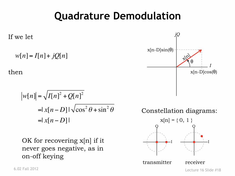
Quadrature Demodulation

If we let

w[n] = I[n]+ jQ[n]

then

w[n]

6.02 Fall 2012 Lecture 16 Slide #18

= I[n]2 +Q[n]2

=| x[n−D] | cos2 θ + sin2 θ

=| x[n−D] |

x[n-D]cos(θ)

x[n-D]sin(θ)

I θ

jQ

Constellation diagrams:

transmitter receiver

I

Q

I

Q

x[n] = { 0, 1 }

OK for recovering x[n] if it never goes negative, as in on-off keying

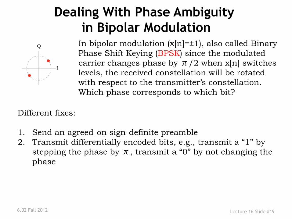
Dealing With Phase Ambiguity in Bipolar Modulation

In bipolar modulation (x[n]=±1), also called Binary Phase Shift Keying (BPSK) since the modulated carrier changes phase by /2 when x[n] switches levels, the received constellation will be rotated with respect to the transmitter’s constellation. Which phase corresponds to which bit?

6.02 Fall 2012 Lecture 16 Slide #19

Q

I

Different fixes: 1.  Send an agreed-on sign-definite preamble 2.  Transmit differentially encoded bits, e.g., transmit a “1” by

stepping the phase by , transmit a “0” by not changing the phase

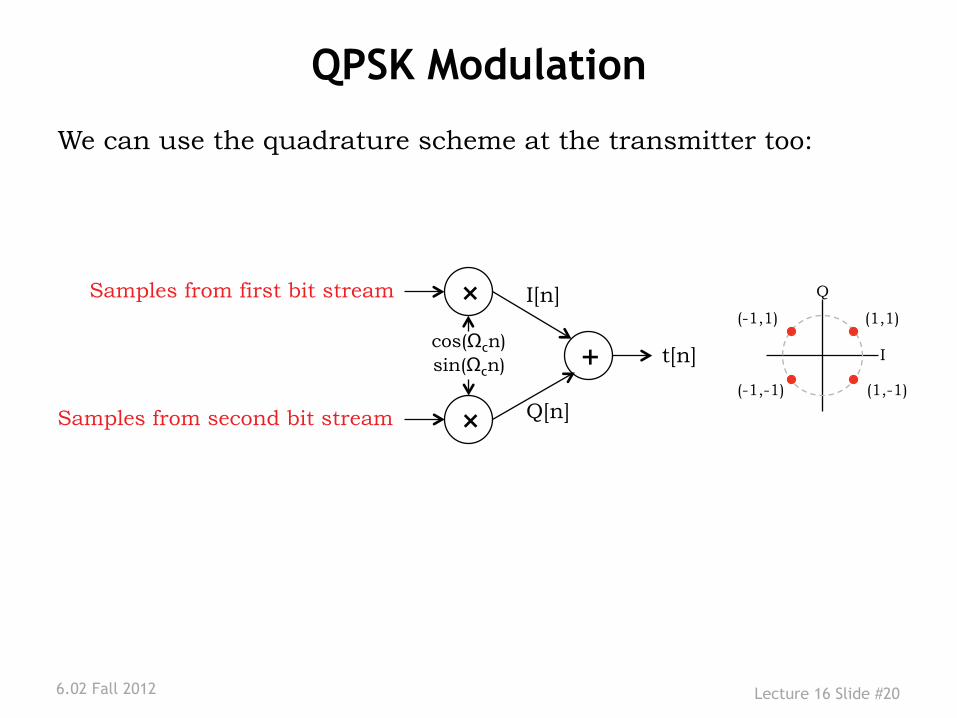
QPSK Modulation

6.02 Fall 2012 Lecture 16 Slide #20

×cos(Ωcn)

×

sin(Ωcn) + t[n]

I[n]

Q[n]

I

Q

(-1,1) (1,1)

(-1,-1) (1,-1)

We can use the quadrature scheme at the transmitter too:

Samples from first bit stream

Samples from second bit stream

http://en.wikipedia.org/wiki/Phase-shift_keying 6.02 Fall 2012 Lecture 16 Slide #21

Phase Shift Keying underlies many familiar modulation schemes

The wireless LAN standard, IEEE 802.11b-1999, uses a variety of different PSKs depending on the data-rate required. At the basic-rate of 1 Mbit/s, it uses DBPSK (differential BPSK). To provide the extended-rate of 2 Mbit/s, DQPSK is used. In reaching 5.5 Mbit/s and the full-rate of 11 Mbit/s, QPSK is employed, but has to be coupled with complementary code keying. The higher-speed wireless LAN standard, IEEE 802.11g-2003 has eight data rates: 6, 9, 12, 18, 24, 36, 48 and 54 Mbit/s. The 6 and 9 Mbit/s modesuse OFDM modulation where each sub-carrier is BPSK modulated. The 12 and 18 Mbit/s modes use OFDM with QPSK. The fastest four modes use OFDM with forms of quadrature amplitude modulation. Because of its simplicity BPSK is appropriate for low-cost passive transmitters, and is used in RFID standards such as ISO/IEC 14443 which has been adopted for biometric passports, credit cards such as American Express's ExpressPay, and many other applications. Bluetooth 2 will use (p/4)-DQPSK at its lower rate (2 Mbit/s) and 8-DPSK at its higher rate (3 Mbit/s) when the link between the two devices is sufficiently robust. Bluetooth 1 modulates with Gaussian minimum-shift keying, a binary scheme, so either modulation choice in version 2 will yield a higher data-rate. A similar technology, IEEE 802.15.4 (the wireless standard used by ZigBee) also relies on PSK. IEEE 802.15.4 allows the use of two frequency bands: 868–915 MHz using BPSK and at 2.4 GHz using OQPSK.

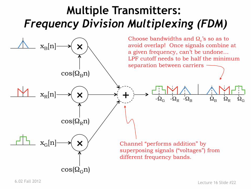
Multiple Transmitters: Frequency Division Multiplexing (FDM)

6.02 Fall 2012

×xB[n]

×xR[n]

×xG[n]

cos(ΩBn)

cos(ΩRn)

cos(ΩGn)

Lecture 16 Slide #22

+

Channel “performs addition” by superposing signals (“voltages”) from different frequency bands.

Choose bandwidths and Ωc’s so as to avoid overlap! Once signals combine at a given frequency, can’t be undone… LPF cutoff needs to be half the minimum separation between carriers

-ΩG -ΩR -ΩB ΩB ΩR ΩG

AM Radio AM radio stations are on 520 – 1610 kHz (‘medium wave”) in the US, with carrier frequencies of different stations spaced 10 kHz apart. Physical effects very much affect operation. e.g., EM signals at these frequencies propagate much further at night (by “skywave” through the ionosphere) than during the day (100’s of miles by “groundwave” diffracting around the earth’s surface), so transmit power may have to be lowered at night!

6.02 Fall 2012 Lecture 16 Slide #23

MIT OpenCourseWarehttp://ocw.mit.edu

6.02 Introduction to EECS II: Digital Communication SystemsFall 2012

For information about citing these materials or our Terms of Use, visit: http://ocw.mit.edu/terms.