6.02 Notes, Chapter 13: Fourier Analysis and Spectral ...

MIT 6.02 DRAFT Lecture Notes Last update: November 3, 2012

CHAPTER 13 Fourier Analysis and Spectral

Representation of Signals

We have seen in the previous chapter that the action of an LTI system on a sinusoidal or complex exponential input signal can be represented effectively by the frequency response H(Ω) of the system. By superposition, it then becomes easy—again using the frequency response—to determine the action of an LTI system on a weighted linear combination of sinusoids or complex exponentials (as illustrated in Example 3 of the preceding chapter). The natural question now is how large a class of signals can be represented in this manner. The short answer to this question: most signals you are likely to be interested in!

The tool for exposing the decomposition of a signal into a weighted sum of sinusoids or complex exponentials is Fourier analysis. We first discuss the Discrete-Time Fourier Transform (DTFT), which we have actually seen hints of already and which applies to the most general classes of signals. We then move to the Discrete-Time Fourier Series (DTFS), which constructs a similar representation for the special case of periodic signals, or for signals of finite duration. The DTFT development provides some useful background, context and intuition for the more special DTFS development, but may be skimmed over on an initial reading (i.e., understand the logical flow of the development, but don’t struggle too much with the mathematical details).

• 13.1 The Discrete-Time Fourier Transform

We have in fact already derived an expression in the previous chapter that has the flavor of what we are looking for. Recall that we obtained the following representation for the unit sample response h[n] of an LTI system:

h[n] = 1 2π

<2π>

H(Ω)ejΩn dΩ , (13.1)

183

184 CHAPTER 13. FOURIER ANALYSIS AND SPECTRAL REPRESENTATION OF SIGNALS

where the frequency response, H(Ω), was defined by

∞ H(Ω) = h[m]e −jΩm . (13.2)

m=−∞

Equation (13.1) can be interpreted as representing the signal h[n] by a weighted combination of a continuum of exponentials, of the form ejΩn, with frequencies Ω in a 2π-range, and associated weights H(Ω) dΩ.

As far as these expressions are concerned, the signal h[n] is fairly arbitrary; the fact that we were considering it as the unit sample response of a system was quite incidental. We only required it to be a signal for which the infinite sum on the right of Equation (13.2) was well-defined. We shall accordingly rewrite the preceding equations in a more neutral notation, using x[n] instead of h[n]:

x[n] = 1 2π <2π>

X(Ω)ejΩn dΩ , (13.3)

where X(Ω) is defined by ∞

X(Ω) = x[m]e −jΩm . (13.4) m=−∞

For a general signal x[·], we refer to the 2π-periodic quantity X(Ω) as the discrete-time Fourier transform (DTFT) of x[·]; it would no longer make sense to call it a frequency response. Even when the signal is real, the DTFT will in general be complex at each Ω.

The DTFT synthesis equation, Equation (13.3), shows how to synthesize x[n] as a weighted combination of a continuum of exponentials, of the form ejΩn, with frequencies Ω in a 2π-range, and associated weights X(Ω) dΩ. From now on, unless mentioned otherwise, we shall take Ω to lie in the range [−π,π].

The DTFT analysis equation, Equation (13.4), shows how the weights are determined. We also refer to X(Ω) as the spectrum or spectral distribution or spectral content of x[·].

Example 1 (Spectrum of Unit Sample Function) Consider the signal x[n] = δ[n], the unit sample function. From the definition in Equation (13.4), the spectral distribution is given by X(Ω) = 1, because x[n] = 0 for all n �= 0, and x[0] = 1. The spectral distribution is thus constant at the value 1 in the entire frequency range [−π,π]. What this means is that it takes the addition of equal amounts of complex exponentials at all frequencies in a 2π-range to synthesize a unit sample function, a perhaps surprising result. What’s happening here is that all the complex exponentials reinforce each other at time n = 0, but effectively cancel each other out at every other time instant.

Example 2 (Phase Matters) What if X(Ω) has the same magnitude as in the previous example, so |X(Ω)| = 1, but has a nonzero phase characteristic, ∠X(Ω) = −αΩ for some α �= 0? This phase characteristic is linear in Ω. With this,

−jαΩ −jαΩX(Ω) = 1.e = e .

Z

�

185 SECTION 13.1. THE DISCRETE-TIME FOURIER TRANSFORM

To find the corresponding time signal, we simply carry out the integration in Equation (13.3). If α is an integer, the integral

yields the value 0 for all n = α. To see this, note that ( ) ( )

j(n−α)Ωe = cos (n − α)Ω + j sin (n − α)Ω ,

and the integral of this expression over any 2π-interval is 0, when n − α is a nonzero integer. However, if n − α = 0, i.e., if n = α, the cosine evaluates to 1, the sine evaluates to 0, and the integral above evaluates to 1. We therefore conclude that when α is an integer,

x[n] = δ[n − α] .

The signal is just a shifted unit sample (delayed by α if α > 0, and advanced by |α| otherwise). The effect of adding the phase characteristic to the case in Example 1 has been to just shift the unit sample in time.

For non-integer α, the answer is a little more intricate:

This time-function is referred to as a “sinc” function. We encountered this function when determining the unit sample response of an ideal lowpass filter in the previous chapter.

Example 3 (A Bandlimited Signal) Consider now a signal whose spectrum is flat but band-limited: {

1 for |Ω| < ΩcX(Ω) = 0 for Ωc ≤ |Ω| ≤ π

The corresponding signal is again found directly from Equation (13.3). For n = 0, we get

x[n] =1

2⇡

Z

<2⇡>e�j↵⌦ej⌦n d⌦ =

1

2⇡

Z

<2⇡>ej(n�↵)⌦ d⌦

x[n] =

1

2⇡

Z ⇡

�⇡e�j↵⌦ej⌦n d⌦

=

1

2⇡

ej(n�↵)⌦

j(n� ↵)

��⇡

�⇡

=

sin

⇣⇡(n� ↵)

⌘

⇡(n� ↵)

x[n] =

1

2⇡

Z

�⌦

c

ej⌦n d⌦

=

1

2⇡

ej⌦

jn

��⌦

c

�⌦

c

=

sin(⌦cn)

⇡n, (13.5)

⌦

c

rsha10

Line

rsha10

Line


which is again a sinc function. For n = 0, Equation (13.3) yields

(This is exactly what we would get from Equation (13.5) if n was treated as a continuous variable, and the limit of the sinc function as n → 0 was evaluated by L’Hopital’s rule—a useful mnemonic, but not a derivation!)

From our study of the analogous equations for h[·] in the previous chapter, we know that the DTFT of x[·] is well-defined when this signal is absolutely summable,

for some μ. However, the DTFT is in fact well-defined for signals that satisfy less demanding constraints, for instance square summable signals,

The sinc function in the examples above is actually not absolutely summable because it follows off too slowly—only as 1/n—as |n| → ∞. However, it is square summable.

A digression: One can also define the DTFT for signals x[n] that do not converge to 0 as |n| → ∞, provided they grow no faster than polynomially in n as |n| → ∞. An example of such a signal of slow growth would be x[n] = ejΩ0n for all n, whose spectrum must be concentrated at Ω = Ω0. However, the corresponding X(Ω) turns out to no longer be an ordinary function, but is a (scaled) Dirac impulse in frequency, located at Ω = Ω0:

X(Ω) = 2πδ(Ω−Ω0) .

You may have encountered the Dirac impulse in other settings. The unit impulse at Ω=Ω0

can be thought of as a “function” that has the value 0 at all points except at Ω=Ω0, and has unit area. This is an instance of a broader result, namely that signals of slow growth possess transforms that are generalized functions (e.g., impulses), which have to be interpreted in terms of what they do under an integral sign, rather than as ordinary functions. It is partly in order to avoid having to deal with impulses and generalized functions in treating sinusoidal and periodic signals that we shall turn to the Discrete-Time Fourier Series rather than the DTFT. End of digression!

We make one final observation before moving to the DTFS. As shown in the previous chapter, if the input x[n] to an LTI system with frequency response H(Ω) is the (everlasting) exponential signal ejΩn, then the output is y[n] = H(Ω)ejΩn. By superposition, if the input is instead the weighted linear combination of such exponentials that is given in Equation (13.3), then the corresponding output must be the same weighted combination of responses, so

x[n] =1

2⇡

Z⌦

c

�⌦

1d⌦ =

⌦c

⇡.

1X

m=�1

��x[m]

�� µ < 1

1X

m=�1

��x[m]

��2

µ < 1 .

y[n] =1

2⇡

Z

<2⇡>H(⌦)X(⌦)ej⌦n d⌦ . (13.6)

187 SECTION 13.2. THE DISCRETE-TIME FOURIER SERIES

However, we also know that the term H(Ω)X(Ω) multiplying the complex exponential in this expression must be the DTFT of y[·], so

Y (Ω) = H(Ω)X(Ω) . (13.7)

Thus, the time-domain convolution relation y[n] = (h∗ x)[n] has been converted to a simple multiplication in the frequency domain. This is a result we saw in the previous chapter too, when discussing the frequency response of a series or cascade combination of two LTI systems: the relation h[n] = (h1 ∗ h2)[n] in the time domain mapped to an overall frequency response of H(Ω) = H1(Ω)H2(Ω) that was simply the product of the individual frequency responses. This is a major reason for the power of frequency-domain analysis; the more involved operation of convolution in time is replaced by multiplication in frequency.

• 13.2 The Discrete-Time Fourier Series

The DTFT synthesis expression in Equation (13.3) expressed x[n] as a weighted sum of a continuum of complex exponentials, involving all frequencies Ω in [−π,π]. Suppose now that x[n] is a periodic signal of (integer) period P , so

x[n+ P ] = x[n]

for all n. This signal is completely specified by the P values it takes in a single period, for instance the values x[0], x[1], . . . , x[P − 1]. It would seem in this case as though we should be able to get away with using a smaller number of complex exponentials to construct x[n] on the interval [0, P − 1] and thereby for all n. The discrete-time Fourier series (DTFS) shows that this is indeed the case.

Before we write down the DTFS, a few words of reassurance are warranted. The expressions below may seem somewhat bewildering at first, with a profusion of symbols and subscripts, but once we get comfortable with what the expressions are saying, interpret them in different ways, and do some examples, they end up being quite straightforward. So don’t worry if you don’t get it all during the first pass through this material—allow yourself some time, and a few visits, to get comfortable!

• 13.2.1 The Synthesis Equation

The essence of the DTFS is the following statement:

Any P -periodic signal x[n] can be represented (or synthesized) as a weighted lin

ear combination of P complex exponentials (or spectral components), where the fre

quencies of the exponentials are located evenly in the interval [−π,π], starting in the middle at the frequency Ω0 = 0 and increasing outwards in both directions in steps of Ω1 = 2π/P .

kn

More concretely, the claim is that any P -periodic DT signal x[n] can be represented in theform

x[n] =X

k=hP i

Akej⌦

k

n , (13.8)

ΩΩ


Ω_1 Ω0 Ω1

–l l0

Ω0 Ω1 Ω2 Ω3 Ω_3 Ω_2 Ω_1

exp(jΩ0)

exp(jΩ_1)

exp(jΩ2)

exp(jΩ3) = exp(jΩ_3)

exp(jΩ1)

exp(jΩ_2)

. 1–1

j

–j

–l 0 l

exp(jΩ1)

. 1–1

j

–j

exp(jΩ0)

exp(jΩ_1)

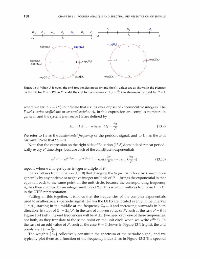
Figure 13-1: When P is even, the end frequencies are at ±π and the Ωk values are as shown in the pictures

on the left for P = 6. When P is odd, the end frequencies are at ±(π − Ω2 1 ), as shown on the right for P = 3.

where we write k = (P ) to indicate that k runs over any set of P consecutive integers. The Fourier series coefficients or spectral weights Ak in this expression are complex numbers in general, and the spectral frequencies Ωk are defined by

2π Ωk = kΩ1 , where Ω1 = . (13.9)

P

We refer to Ω1 as the fundamental frequency of the periodic signal, and to Ωk as the k-th harmonic. Note that Ω0 = 0.

Note that the expression on the right side of Equation (13.8) does indeed repeat periodically every P time steps, because each of the constituent exponentials

2π 2πjΩkn jkΩ1n e = e = ejkn(2π/P ) = cos(k n) + j sin(k n) (13.10)P P

repeats when n changes by an integer multiple of P . It also follows from Equation (13.10) that changing the frequency index k by P — or more

generally by any positive or negative integer multiple of P — brings the exponential in that equation back to the same point on the unit circle, because the corresponding frequency Ωk has then changed by an integer multiple of 2π. This is why it suffices to choose k = (P ) in the DTFS representation.

Putting all this together, it follows that the frequencies of the complex exponentials used to synthesize a P -periodic signal x[n] via the DTFS are located evenly in the interval [−π,π], starting in the middle at the frequency Ω0 = 0 and increasing outwards in both directions in steps of Ω1 = 2π/P . In the case of an even value of P , such as the case P = 6 in Figure 13-1 (left), the end frequencies will be at ±π (we need only one of these frequencies, not both, as they translate to the same point on the unit circle when we write ejΩkn). In the case of an odd value of P , such as the case P = 3 shown in Figure 13-1 (right), the end points are ±(π − Ω1 ).2

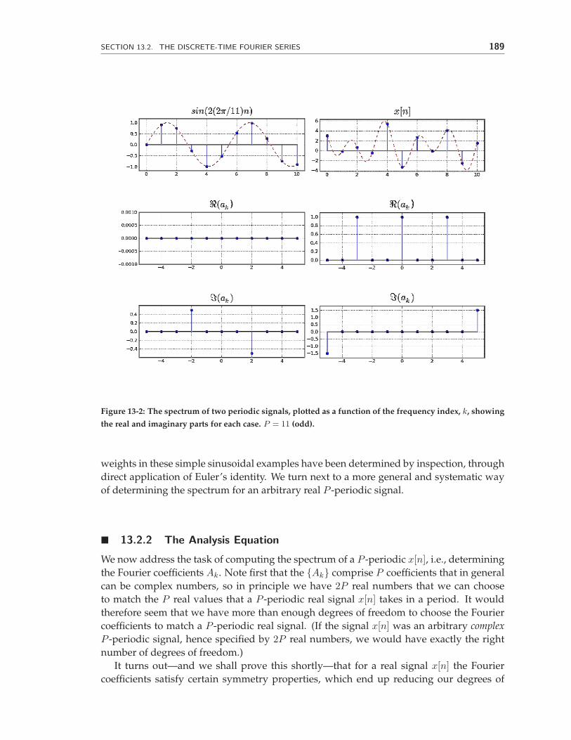
The weights {Ak} collectively constitute the spectrum of the periodic signal, and we typically plot them as a function of the frequency index k, as in Figure 13-2 The spectral


Figure 13-2: The spectrum of two periodic signals, plotted as a function of the frequency index, k, showing

the real and imaginary parts for each case. P = 11 (odd).

weights in these simple sinusoidal examples have been determined by inspection, through direct application of Euler’s identity. We turn next to a more general and systematic way of determining the spectrum for an arbitrary real P -periodic signal.

• 13.2.2 The Analysis Equation

We now address the task of computing the spectrum of a P -periodic x[n], i.e., determining the Fourier coefficients Ak. Note first that the {Ak} comprise P coefficients that in general can be complex numbers, so in principle we have 2P real numbers that we can choose to match the P real values that a P -periodic real signal x[n] takes in a period. It would therefore seem that we have more than enough degrees of freedom to choose the Fourier coefficients to match a P -periodic real signal. (If the signal x[n] was an arbitrary complex P -periodic signal, hence specified by 2P real numbers, we would have exactly the right number of degrees of freedom.)

It turns out—and we shall prove this shortly—that for a real signal x[n] the Fourier coefficients satisfy certain symmetry properties, which end up reducing our degrees of


freedom to precisely P rather than 2P . Specifically, we can show that

Ak = A ∗ (13.11)−k ,

so the real part of Ak is an even function of k, while the imaginary part of Ak is an odd function of k. This also implies that A0 is purely real, and also that in the case of even P , the values AP/2 = A−P/2 are purely real. (These properties should remind you of the symmetry properties we exposed in connection with frequency responses in the previous chapter — but that’s no surprise, because the DTFS is a similar kind of object.)

Making a careful count now of the actual degrees of freedom, we find that it takes precisely P real parameters to specify the spectrum {Ak} for a real P -periodic signal. So given the P real values that x[n] takes over a single period, we expect that Equation (13.8) will give us precisely P equations in P unknowns. (For the case of a complex signal, we will get 2P equations in 2P unknowns.)

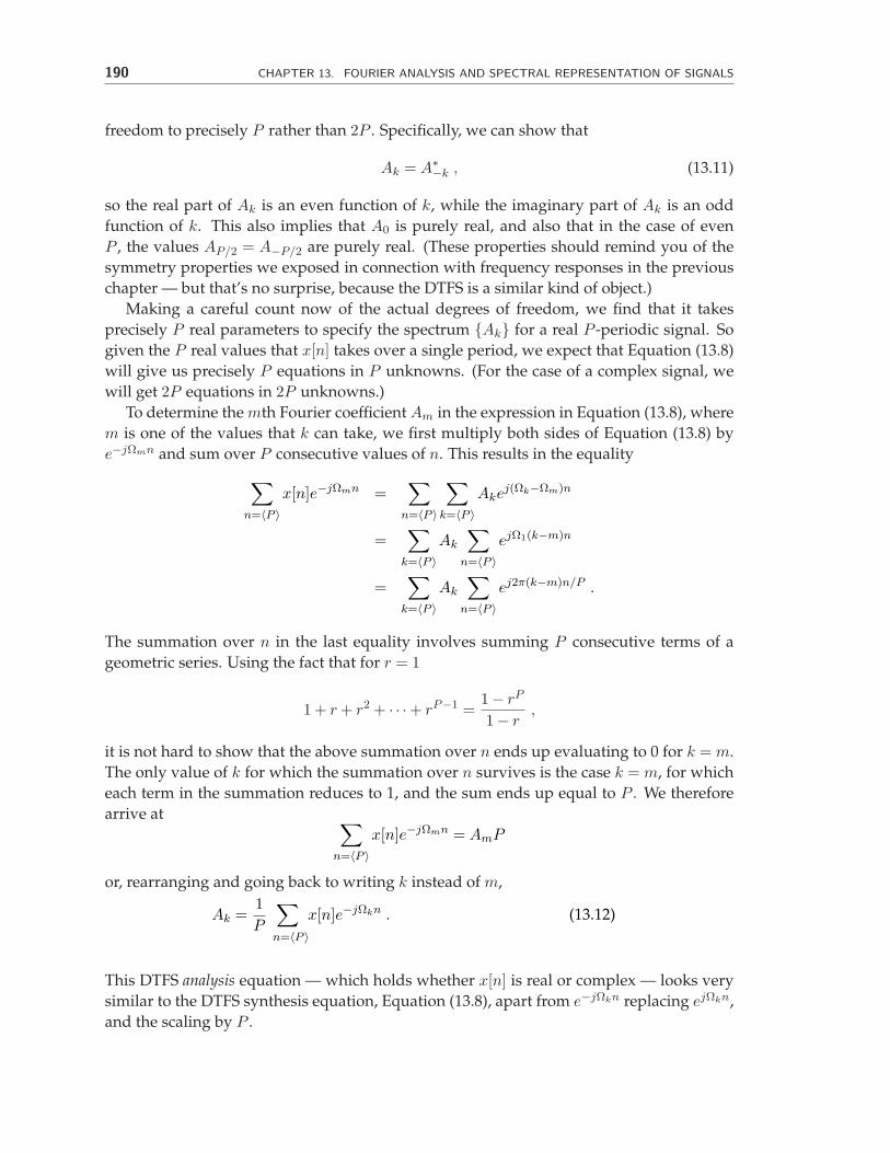
To determine the mth Fourier coefficient Am in the expression in Equation (13.8), where m is one of the values that k can take, we first multiply both sides of Equation (13.8) by e−jΩmn and sum over P consecutive values of n. This results in the equality

The summation over n in the last equality involves summing P consecutive terms of a geometric series. Using the fact that for r = 1

P1− r2 P −11 + r + r + · · ·+ r = ,1− r

it is not hard to show that the above summation over n ends up evaluating to 0 for k = m. The only value of k for which the summation over n survives is the case k = m, for which each term in the summation reduces to 1, and the sum ends up equal to P . We therefore arrive at

or, rearranging and going back to writing k instead of m,

This DTFS analysis equation — which holds whether x[n] is real or complex — looks very similar to the DTFS synthesis equation, Equation (13.8), apart from e−jΩkn replacing ejΩkn , and the scaling by P .

x en

X[n] �j⌦

m

n=

=hP i n

X

=hP i k

XAke

j(⌦k

�⌦

m

)n

=hP i

=

XA

Xej⌦1(k

k�m)n

k=hP i n=hP i

=

XA

Xej2⇡(k m

k� )n/P .

k=hP i n=hP i

1

Ak = x[n]e�j⌦k

n .P

X(13.12)

Xx[n]e m

= AmPn=hP i

�j⌦ n

n=hP i


Two particular observations that follow directly from the analysis formula:

1 A0 = x[n] , (13.13)

P n=(P )

and, for the case of even P , where ΩP/2 = π,

AP/2 = A−P/2 =1

(−1)n x[n] . (13.14)P

n=(P )

The symmetry properties of Ak that we stated earlier in the case of a real signal follow directly from this analysis equation, as we leave you to verify. Also, since A−k = A∗ for a k real signal, we can combine the terms

−jΩkn jΩknAke + Ake

into the single term 2|Ak| cos(Ωkn + ∠Ak) .

Thus, for even P , P/2

x[n] = A0 + 2|Ak| cos(Ωkn + ∠Ak) , k=1

while for odd P the only change is that the upper limit becomes (P − 1)/2.

• 13.2.3 The Aperiodic Limit, P →∞

There is a slightly modified form in which the DTFS is sometimes written:

1 jΩk n x[n] = Xke , (13.15)P

k=(P )

which just corresponds to working with a scaled version of the Ak that we have used so far, namely

−jΩknXk = PAk = x[n]e . (13.16) n=(P )

This form of the DTFS is useful when one considers the limiting case of aperiodic signals by letting P → ∞, (2π/P ) → dΩ, and Ωk → Ω. In this limiting case, it is easy to deduce from Equation (13.12) that Xk → X(Ω), precisely the DTFT of the aperiodic signal that we defined in Equation (13.4). Correspondingly, the DTFS synthesis equation, Equation (13.8), in this limiting case becomes precisely the expression in Equation (13.3).

• 13.2.4 Action of an LTI System on a Periodic Input

Suppose the input x[·] to an LTI system with frequency response H(Ω) is P -periodic. This signal can be represented as a weighted sum of exponentials, by the DTFS in Equation

X

X

X

X

X


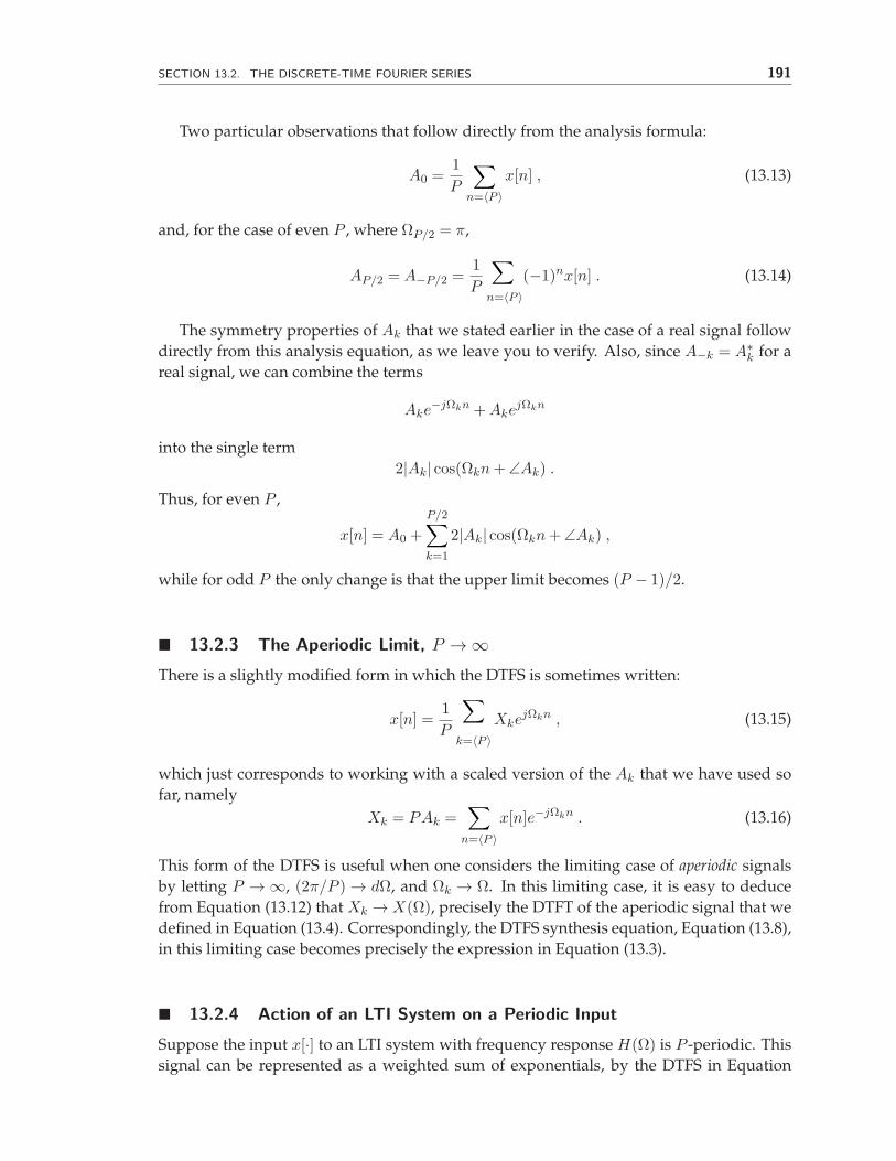
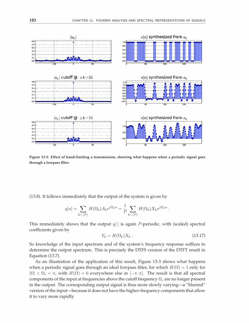
Figure 13-3: Effect of band-limiting a transmission, showing what happens when a periodic signal goes

through a lowpass filter.

(13.8). It follows immediately that the output of the system is given by

1jΩkn jΩkn y[n] = H(Ωk)Ake = H(Ωk)Xke . P

k=(P ) k=(P )

This immediately shows that the output y[·] is again P -periodic, with (scaled) spectral coefficients given by

Yk = H(Ωk)Xk . (13.17)

So knowledge of the input spectrum and of the system’s frequency response suffices to determine the output spectrum. This is precisely the DTFS version of the DTFT result in Equation (13.7).

As an illustration of the application of this result, Figure 13-3 shows what happens when a periodic signal goes through an ideal lowpass filter, for which H(Ω) = 1 only for |Ω| < Ωc < π, with H(Ω) = 0 everywhere else in [−π,π]. The result is that all spectral components of the input at frequencies above the cutoff frequency Ωc are no longer present in the output. The corresponding output signal is thus more slowly varying—a “blurred” version of the input—because it does not have the higher-frequency components that allow it to vary more rapidly.

X X


• 13.2.5 Application of the DTFS to Finite-Duration Signals

The DTFS turns out to be useful in settings that do not involve periodic signals, but rather signals of finite duration. Suppose a signal x[n] takes nonzero values only on some finite interval, say [0, P − 1] for example. We are not forbidding x[n] from taking the value 0 for n within this interval, but are saying that x[n] = 0 for all n outside this interval. If we now compute the DT Fourier transform of this signal, according to the definition in Equation (13.4), we get

P −1

X(Ω) = x[n]e −jΩn . (13.18) n=0

The corresponding representation of x[n] by a weighted combination of complex exponentials would then be the expression in Equation (13.3), involving a continuum of frequencies. However, it is possible to get a more economical representation of x[n] by using the DT Fourier series.

In order to do this, consider the new signal xP [·] obtained by taking the portion of x[·] that lies in the interval [0, P − 1] and replicating it periodically outside this interval, with period P . This results in xP [n+ P ] = xP [n] for all n, with xP [n] = x[n] for n in the interval [0, P − 1]. We can represent this periodic signal by its DTFS:

xP [n] = 1

XkejΩkn , (13.19)

P k=<P >

where P −1

−jΩkn −jΩknXk = xP [n]e = x[n]e . (13.20) n=<P> n=0

(For consistency, we should perhaps have used the notation XPk instead of Xk, but we are trying to keep our notation uncluttered.)

We can now represent x[n] by the expression in Equation (13.19), in terms of just P complex exponentials at the frequencies Ωk defined earlier (in our development of the DTFS), rather than complex exponentials at a continuum of frequencies. However, this representation only captures x[n] in the interval [0, P − 1]. Outside of this interval, we have to ignore the expression, instead invoking our knowledge that x[n] is actually 0 outside.

Another observation worth making from Equations (13.18) and (13.20) is that the (scaled) DTFS coefficients Xk are actually simply related to the DTFT X(Ω) of the finite-duration signal x[n]:

Xk = X(Ωk) , (13.21)

so the (scaled) DTFS coefficients Xk are just P samples of the DTFT X(Ω). Thus any method for computing the DTFS for (the periodic extension of) a finite-duration signal will yield samples of the DTFT of this finite-duration signal (keep track of our use of DTFS versus DTFT here!). And if one wants to evaluate the DTFT of this finite-duration signal at a larger number of sample points, all that needs to be done is to consider x[n] to be of finite-duration on a larger interval, of length P i > P , where of course the additional signal values in the larger interval will all be 0; this is referred to a zero-padding. Then computing the DTFS of (the periodic extension of) x[n] for this longer interval will yield P i samples of the

X

X

X X


underlying DTFT of the signal. As an application of the above results on finite-duration signals, consider the case of

an LTI system whose unit sample response h[n] is known to be 0 for all n outside of some interval [0, nh], and whose input x[n] is known to be 0 for all n outside some interval [0, nx]. It follows that the earliest time instant at which a nonzero output value can appear is n = 0, while the latest such time instant is n = nx + nh. In other words, the response y[n] = (h ∗ x)[n] is guaranteed to be 0 for all n outside of the interval [0, nx + nh]. All the interesting input/output action of the system therefore takes place for n in this interval. Outside of this interval we know that x[·] and y[·] are both 0. We can therefore take all the signals of interest to have finite duration, being 0 outside of the interval [0, P − 1], where P = nx + nh + 1. A DTFS representation of x[·] and y[·] on this interval, with this choice of P , can then be used to carry out a frequency-domain analysis of the system. In particular, the kth (scaled) Fourier coefficients of the input and output will be related as in Equation (13.17).

• 13.2.6 The FFT

Implementing either the DTFS synthesis computation or the DTFS analysis computation, as defined earlier, would seem to require on the order of P 2 multiply/add operations: we have to do P multiply/adds for each of P frequencies. This can quickly lead to prohibitively expensive computations in large problems.

Happily, in 1965 Cooley and Tukey published a fast method for computing these DTFS expressions (rediscovering a technique known to Gauss!). Their algorithm is termed the Fast Fourier Transform or FFT, and takes on the order of P log P operations, which is a big saving. (Note that the FFT is not a new kind of transform, despite its name! — it’s a fast algorithm for computing a familiar transform, namely the DTFS.)

The essence of the idea is to recursively split the computation into a DTFS computation involving the signal values at the even time instants and another DTFS computation involving the signal values at the odd time instants. One then cleverly uses the nice algebraic properties of the P complex exponentials involved in these computations to stitch things back together and obtain the desired DTFS.

The FFT has become a (or maybe the) workhorse of practical numerical computation. Its most common application is to computing samples of the DTFT of finite-duration signals, as described in the previous subsection. It can also be applied, of course, to computing the DTFS of a periodic signal.

• Acknowledgments

Thanks to Patricia Saylor, Kaiying Liao, and Michael Sanders for bug fixes.

• Problems and Questions

1. Let x[·] be a signal that is periodic with period P = 12. For each of the following x[.], give the corresponding spectral coefficients Ak for the discrete-time Fourier series for x[·], for k in the range −6 ≤ k ≤ 6. (Hint: In most of the following cases, all you need to do is express the signal as the sum of appropriate complex exponentials, by


inspection—this is much easier than cranking through the formal definition of the spectral coefficient.)

(a) Determine Ak when x[0 : 11] = [0,0,1,0,0,0,0,0,0,0,0,0].

(b) Determine Ak when x[n] = 1 for all n.

(c) Determine Ak when x[n] = sin(r(2π/12)n) for the following two choices of r:

i. r = 3; and

ii. r = 8.

(d) Determine Ak when x[n] = sin(3(2π/12)n + φ) where φ is some specified phase offset.

2. Consider a lowpass LTI communication channel with input x[n], output y[n], and frequency response H(Ω) given by

−j3ΩH(Ω) = e for 0 ≤ |Ω| < Ωm ,

= 0 for Ωm ≤ |Ω| ≤ π .

Here Ωm denotes the cutoff frequency of the channel; the output y[n] will contain no frequency components in the range Ωm ≤ |Ω| ≤ π. The different parts of this problem involve different choices for Ωm.

(a) Picking Ωm = π/4, provide separate and properly labeled sketches of the magnitude |H(Ω)| and phase ∠H(Ω) of the frequency response, for Ω in the interval 0 ≤ |Ω| ≤ π. (Sketch the phase only in the frequency ranges where |H(Ω)| > 0.)

(b) Suppose Ωm = π, so H(Ω) = e−j3Ω for all Ω in [−π,π], i.e., all frequency components make it through the channel. For this case, y[n] can be expressed quite simply in terms of x[.]; find the relevant expression.

(c) Suppose the input x[n] to this channel is a periodic “rectangular-wave” signal with period 12. Specifically:

x[−1] = x[0] = x[1] = 1

and these values repeat every 12 steps, so

x[11] = x[12] = x[13] = 1

and more generally

x[12r − 1] = x[12r] = x[12r + 1]

for all integers r from −∞ to ∞. At all other times n, we have x[n] = 0. (You might find it helpful to sketch this signal for yourself, e.g., for n ranging from −2 to 13.)


Find explicit values for the Fourier coefficients in the discrete-time Fourier series (DTFS) for this input x[n], i.e., the numbers Ak in the representation

5 jΩkn x[n] = Ake ,

k=−6

where Ωk = k(2π/12). Recall that

1 −jΩk nAk = x[n]e ,12 (n)

where the summation is over any 12 consecutive values of n (as indicated by writing (n)), so all you need to do is evaluate this expression for the particular x[n] that we have. Since x[n] is an even function of n, all the Ak should be purely real, so be sure your expression for Ak makes clear that it is real. (Depending on how you proceed,

−j11(2π/12) j(2π/12).)you may or may not find it helpful to note that e = e

Check that your values for A0 and A−6 = A6 are correct, and be explicit about how you are checking.

(d) Suppose the cutoff frequency of the channel is Ωm = π/4 (which is the case you sketched in part (a), and the input is the x[n] specified in part (c). Compute the values of all the nonzero Fourier coefficients of the channel output y[n], i.e., find the values of the nonzero numbers Bk in the representation

5 jΩkn y[n] = Bke ,

k=−6

where Ωk = k(2π/12). Don’t forget that H(Ω) = e−j3Ω in the passband of the filter, 0 ≤ |Ω| < Ωm.

(e) Express the y[n] in part (d) as an explicit and real function of time n. (If you were to sketch y[n], you would discover that it is a low-frequency approximation to the y[n] that would have been obtained if Ωm = π.)

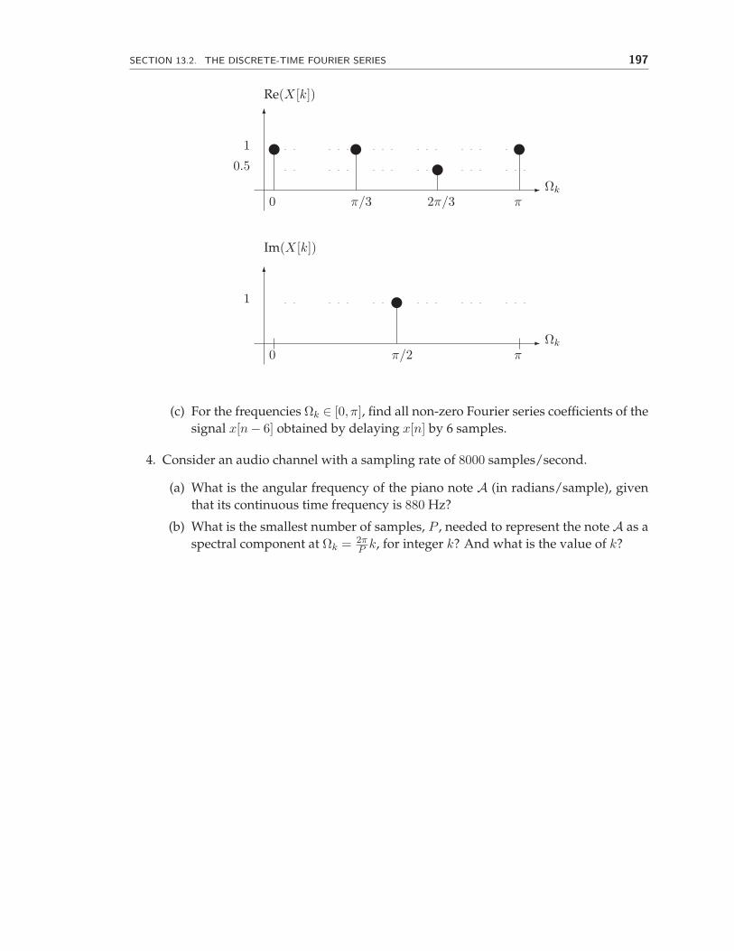
3. The figure below shows the real and imaginary parts of all non-zero Fourier series coefficients X[k] of a real periodic discrete-time signal x[n], for frequencies Ωk ∈ [0, π]. Here Ωk = k(2π/N) for some fixed even integer N , as in all our analysis of the discrete-time Fourier series (DTFS), but the plots below only show the range 0 ≤ k ≤ N/2.

(a) Find all non-zero Fourier series coefficients of x[n] at Ωk in the interval [−π,0), i.e., for −(N/2) ≤ k < 0. Give your answer in terms of careful and fully labeled plots of the real and imaginary parts of X[k] (following the style of the figure above).

(b) Find the period of x[n], i.e., the smallest integer T for which x[n + T ] = x[n], for all n.

X

X

X


Re(X[k])

+

�

Ωk

1

0 π/3 2π/3 π

0.5

Im(X[k])

+

�

Ωk

1

0 π/2 π

(c) For the frequencies Ωk ∈ [0, π], find all non-zero Fourier series coefficients of the signal x[n − 6] obtained by delaying x[n] by 6 samples.

4. Consider an audio channel with a sampling rate of 8000 samples/second.

(a) What is the angular frequency of the piano note A (in radians/sample), given that its continuous time frequency is 880 Hz?

(b) What is the smallest number of samples, P , needed to represent the note A as a 2πspectral component at Ωk = k, for integer k? And what is the value of k?P

MIT OpenCourseWarehttp://ocw.mit.edu

6.02 Introduction to EECS II: Digital Communication SystemsFall 2012

For information about citing these materials or our Terms of Use, visit: http://ocw.mit.edu/terms.

http://ocw.mit.edu/terms

http://ocw.mit.edu

6.02 Notes, Chapter 13: Fourier Analysis and Spectral ...

Documents

Transcript of 6.02 Notes, Chapter 13: Fourier Analysis and Spectral ...