Theory of the Firm

Moshe Ben-Akiva

1.201 / 11.545 / ESD.210Transportation Systems Analysis: Demand & Economics

Fall 2008

Outline

● Basic Concepts

● Production functions

● Profit maximization and cost minimization

● Average and marginal costs

2

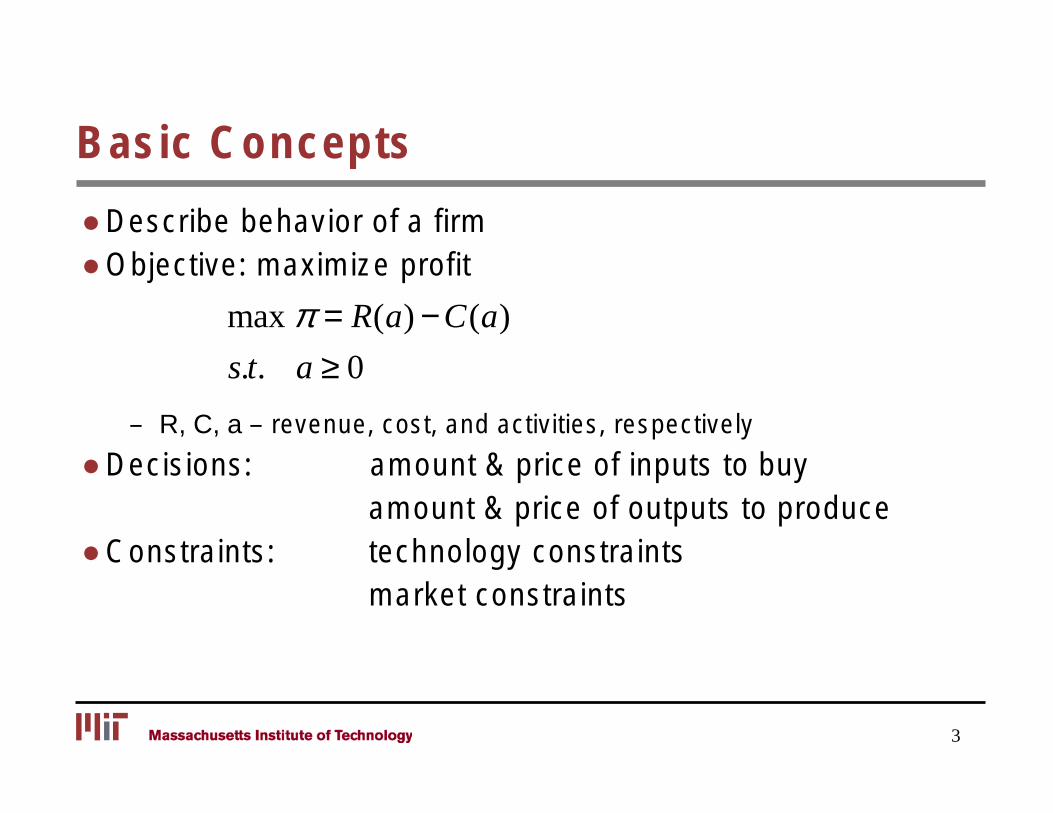
Basic Concepts

● Describe behavior of a firm ● Objective: maximize profit

− ( ) max π = R a ( ) C a

s t . . a ≥ 0

– R, C, a – revenue, cost, and activities, respectively

● Decisions: amount & price of inputs to buy amount & price of outputs to produce

● Constraints: technology constraints market constraints

3

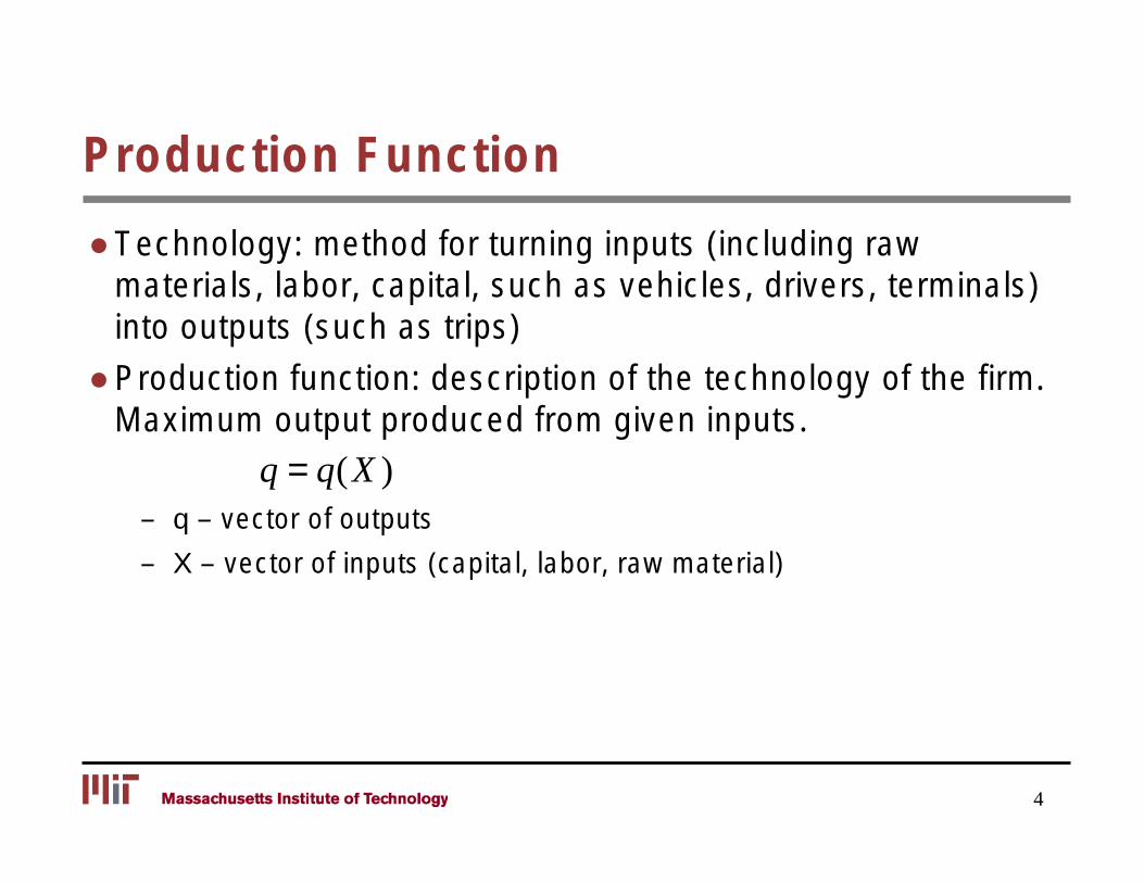
Production Function

● Technology: method for turning inputs (including raw materials, labor, capital, such as vehicles, drivers, terminals) into outputs (such as trips)

● Production function: description of the technology of the firm. Maximum output produced from given inputs.

q = q(X ) – q – vector of outputs

– X – vector of inputs (capital, labor, raw material)

4

Using a Production Function

● The production function predicts what resources are needed to provide different levels of output

● Given prices of the inputs, we can find the most efficient (i.e. minimum cost) way to produce a given level of output

5

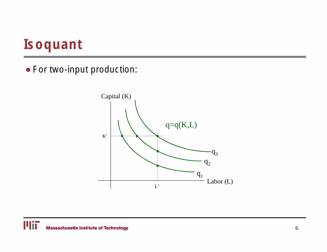
Isoquant

● For two-input production:

Labor (L)

Capital (K)

q1

K’

L’

q=q(K,L)

q2

q3

6

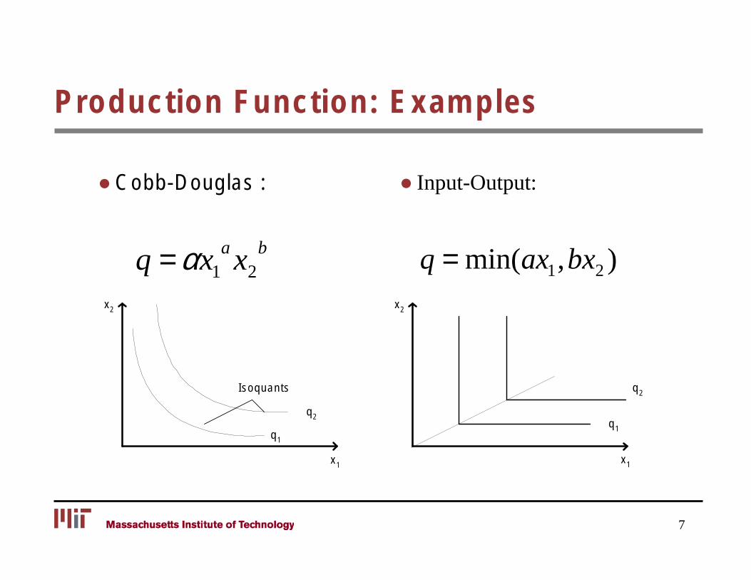
Production Function: Examples

● Cobb-Douglas : ● Input-Output:

q = αx1 a x2

b q = min( ax 1,bx 2 ) x2

q1

x1

Isoquants q2

q2 q1

x1

x2

7

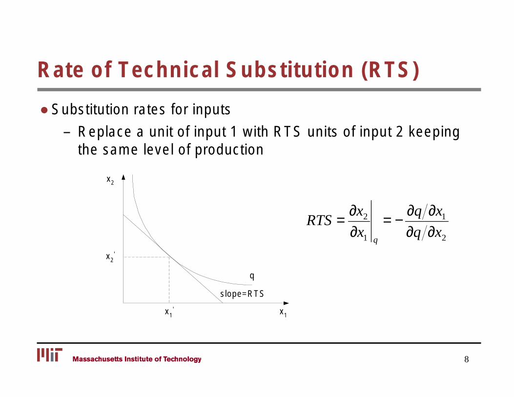
Rate of Technical Substitution (RTS)

● Substitution rates for inputs

– Replace a unit of input 1 with RTS units of input 2 keeping the same level of production

x2

∂x2 ∂q ∂x1RTS = = − ∂x ∂q ∂x21 q

' x2

q

slope=RTS

' x1 x1

8

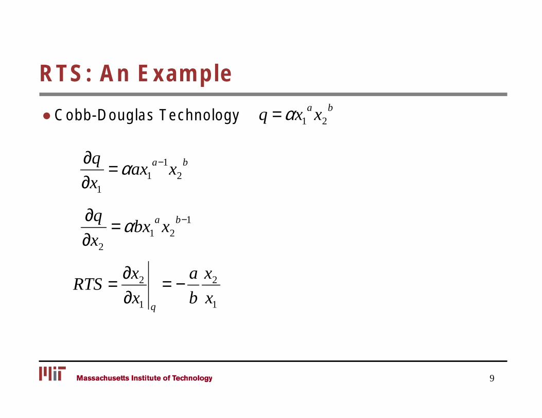
RTS: An Example

● Cobb-Douglas Technology q = αx1 a x2

b

∂q = αax 1 a−1 x2

b

∂x1

∂∂ x

q

2

= αbx 1 a x2

b−1

∂xRTS = 2 = − a x2

∂x b x11 q

9

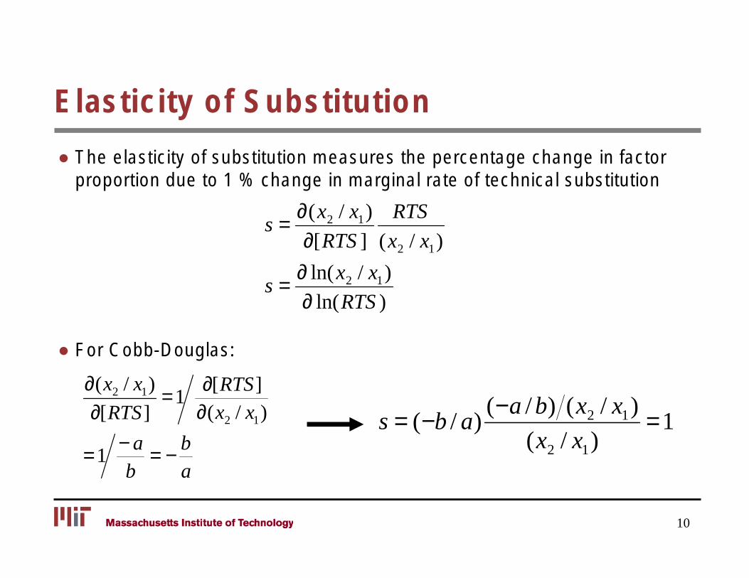
Elasticity of Substitution

● The elasticity of substitution measures the percentage change in factor proportion due to 1 % change in marginal rate of technical substitution

∂(x2 / x1) RTS s =

∂[RTS ] (x2 / x1)

∂ ln( x2 / x1)s =

∂ ln( RTS )

● For Cobb-Douglas:

∂(x2 / x1) = ∂[RTS ]

1

s = (−b / a)(−a / b) (x2 / x1) = 1∂[RTS ]

1 ∂(x2 / x1)

− a b (x2 / x1)= = −

b a

10

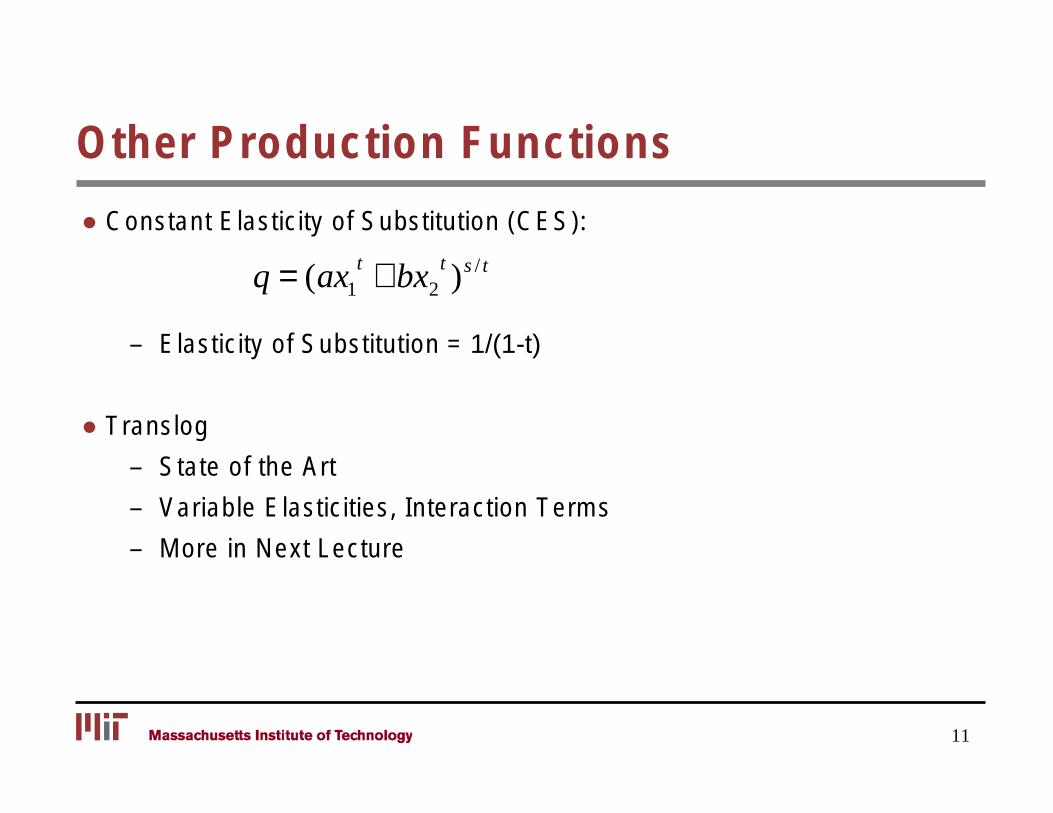
Other Production Functions

● Constant Elasticity of Substitution (CES):

q = (ax 1 t + bx 2

t )s / t

– Elasticity of Substitution = 1/(1-t)

● Translog

– State of the Art

– Variable Elasticities, Interaction Terms

– More in Next Lecture

11

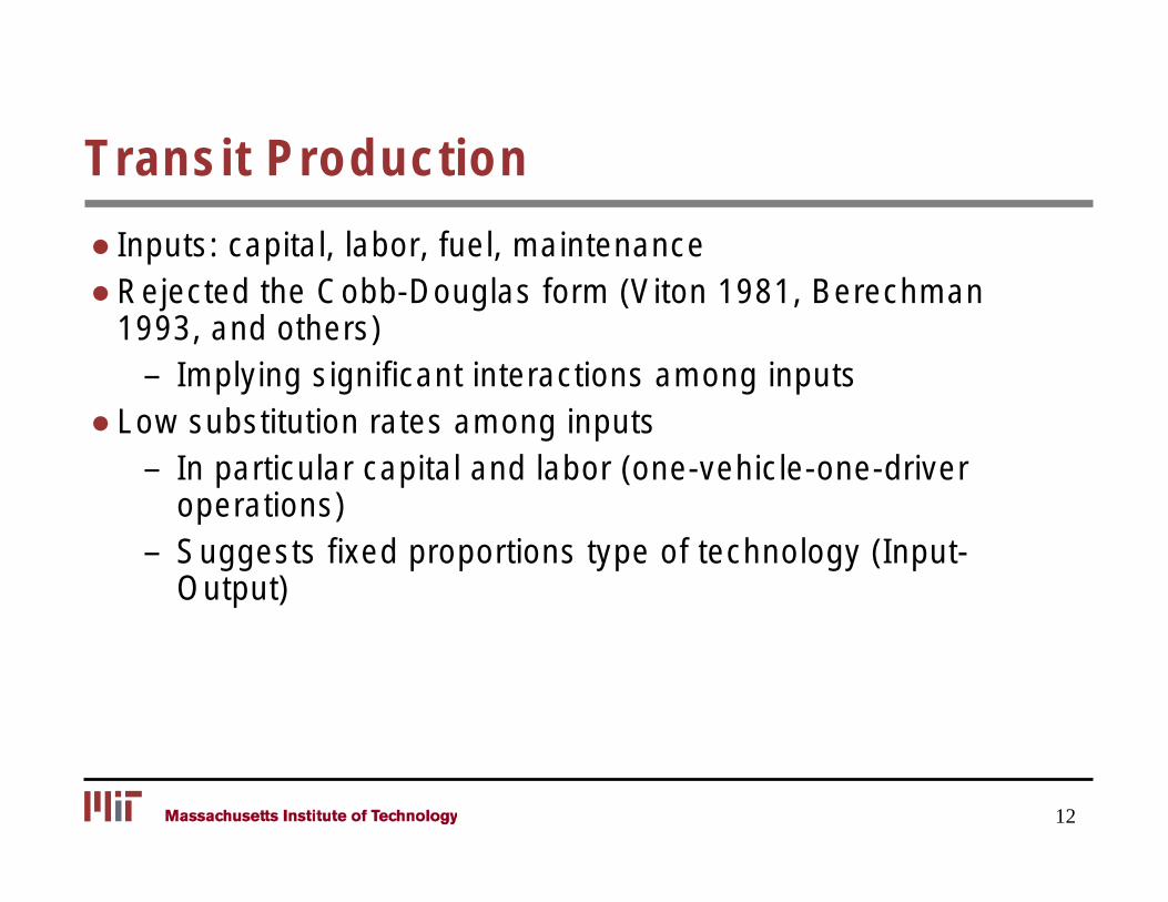
Transit Production

● Inputs: capital, labor, fuel, maintenance ● Rejected the Cobb-Douglas form (Viton 1981, Berechman

1993, and others) – Implying significant interactions among inputs

● Low substitution rates among inputs – In particular capital and labor (one-vehicle-one-driver

operations) – Suggests fixed proportions type of technology (Input-

Output)

12

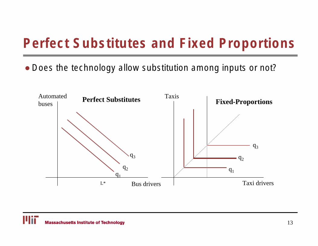
Perfect Substitutes and Fixed Proportions

● Does the technology allow substitution among inputs or not?

Automated Taxis Perfect Substitutes Fixed-Proportions buses

q3

q3 q2

q2 q1 q1

L* Bus drivers Taxi drivers

13

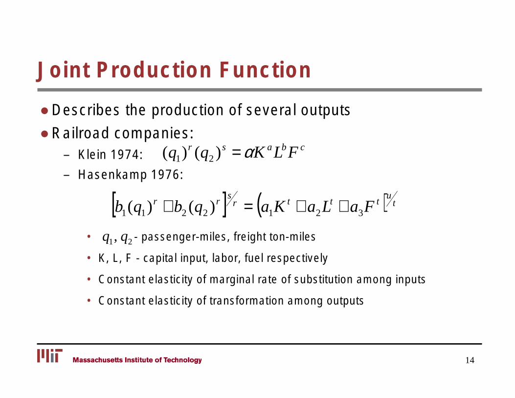
Joint Production Function

● Describes the production of several outputs

● Railroad companies: – Klein 1974: (q1)r (q2 )s = αK aLbF c

– Hasenkamp 1976:

) tu

r rs

r t t t[b (q ) + b (q ) ] = (a K + a L + a F1 1 2 2 1 2 3

• q1, q2 - passenger-miles, freight ton-miles

• K, L, F - capital input, labor, fuel respectively

• Constant elasticity of marginal rate of substitution among inputs

• Constant elasticity of transformation among outputs

14

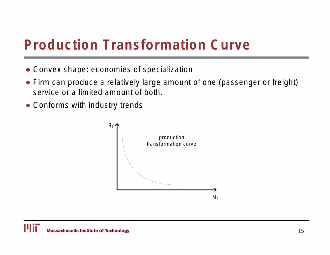
Production Transformation Curve

● Convex shape: economies of specialization

● Firm can produce a relatively large amount of one (passenger or freight) service or a limited amount of both.

● Conforms with industry trends

q2

production transformation curve

q1

15

Outline

● Basic Concepts

● Production functions

● Profit maximization and cost minimization

● Average and marginal costs

16

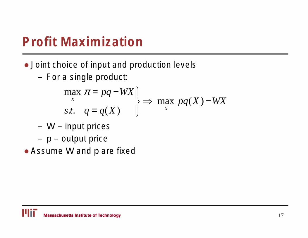
Profit Maximization

● Joint choice of input and production levels – For a single product:

max π = pq −WX x ⇒ max pq X ( ) −WX xs t . . q = ( q X )

– W – input prices – p – output price

● Assume W and p are fixed

17

The Competitive Firm

● Price taker does not influence input and output prices

● Applies when:

– Large number of selling firms

– Identical products

– Well informed customers

18

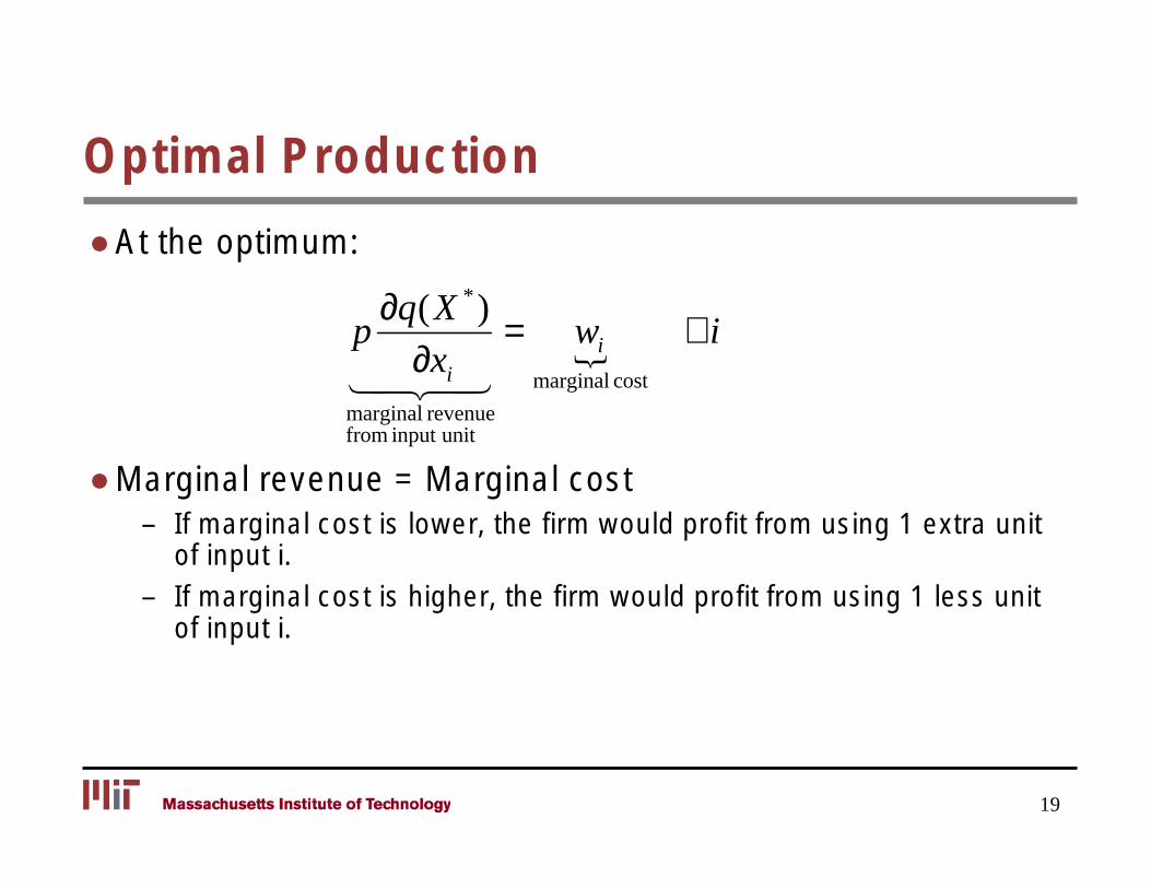
Optimal Production

● At the optimum:

∂q(X *)p = wi ∀i

∂x {i marginal cost 142 43

marginal revenuefrom input unit

● Marginal revenue = Marginal cost – If marginal cost is lower, the firm would profit from using 1 extra unit

of input i. – If marginal cost is higher, the firm would profit from using 1 less unit

of input i.

19

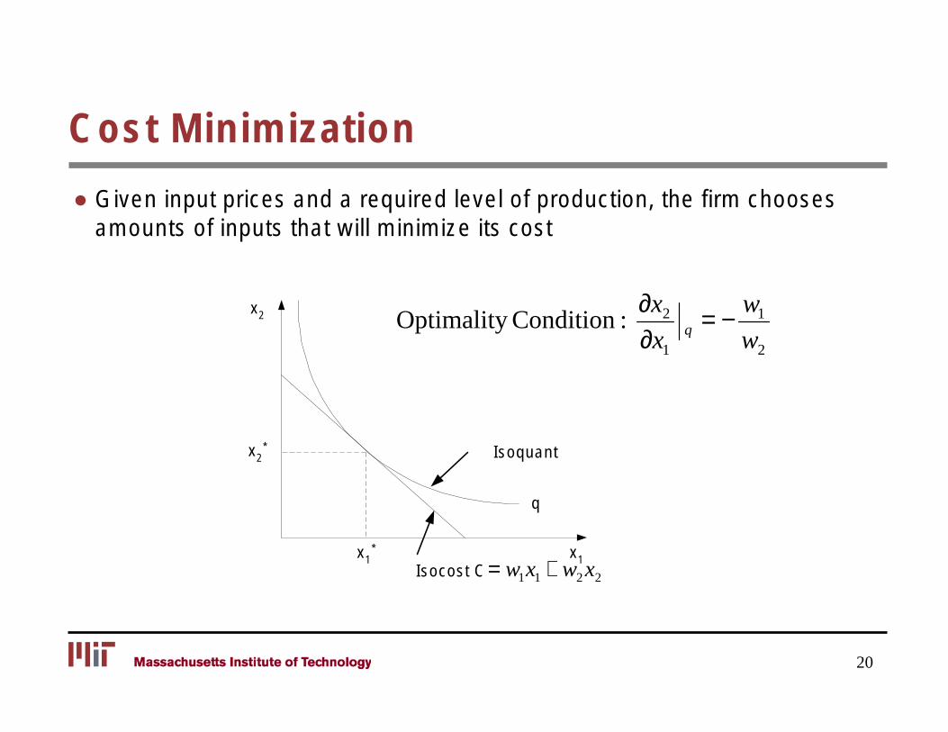
Cost Minimization

● Given input prices and a required level of production, the firm chooses amounts of inputs that will minimize its cost

x1 * x1

x2 *

x2

Isoquant

q

:Condition Optimality ∂x2 = − w1

q∂x1 w2

Isocost C = w1x1 + w2 x2

20

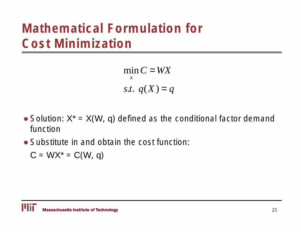
Mathematical Formulation for Cost Minimization

min C = WXx

s.t. q(X ) = q

● Solution: X* = X(W, q) defined as the conditional factor demand function

● Substitute in and obtain the cost function:

C = WX* = C(W, q)

21

Dual Views of the Same Problem

● Production problem: maximize production given level of cost

● Cost problem: minimize cost given a desired level of production.

22

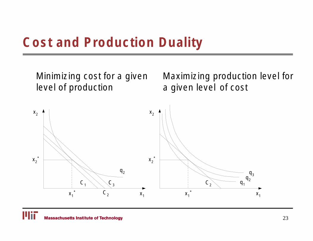
Cost and Production Duality

Minimizing cost for a given Maximizing production level for level of production a given level of cost

x2 *

x2

q2

C3C1

x2 *

x2

C2 q1

q2

q3

x1* C2 x1 x1

* x1

23

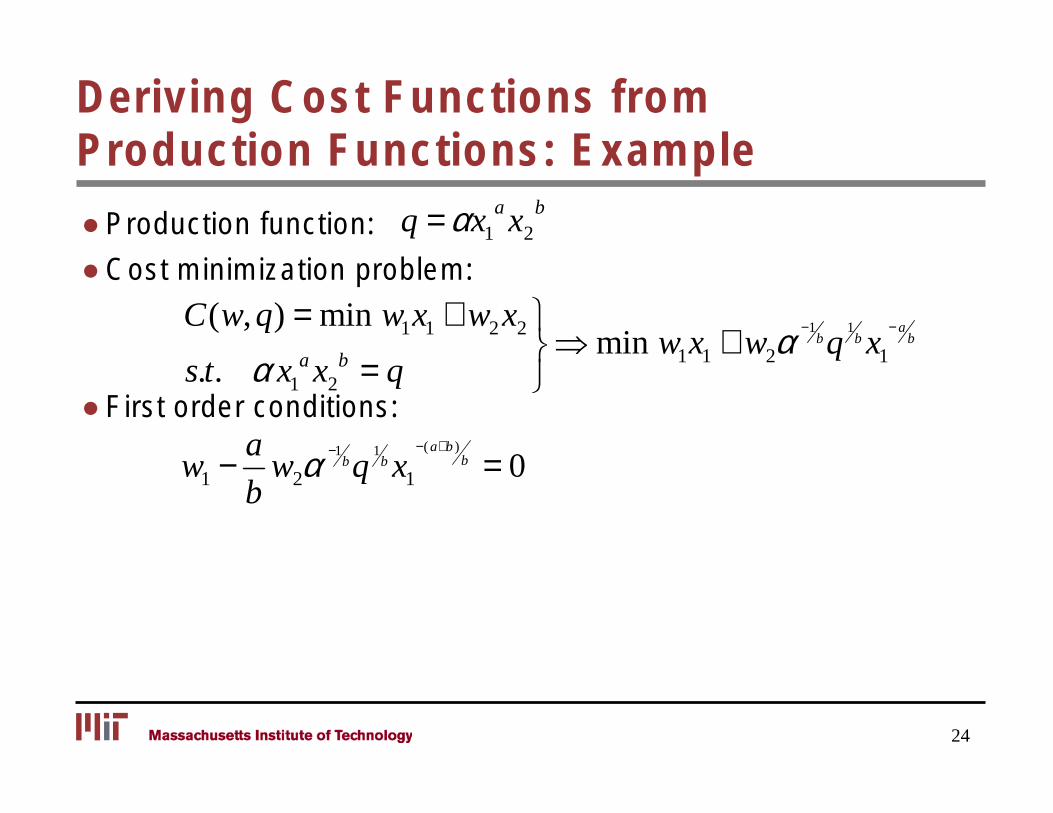
Deriving Cost Functions from Production Functions: Example

● Production function: q = αx1 a x2

b

● Cost minimization problem:

( , ) = min w x + w x −C w q 1 1 2 2 ⇒ min w x + w α −1

bq 1

b x a

b

a bs t . . α x1 x2 = q

1 1 2 1

● First order conditions:

w2α1

bq 1

b x1

−( a+b

w1 − a − ) b = 0

b

24

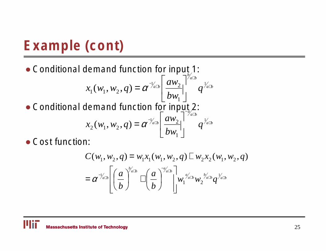
Example (cont)

● Conditional demand function for input 1: aw 2 a+b

b

= α −1 a a

1

( 1 2 , q) b b+ +x1 w , w q

● Conditional demand function for input 2:

a−

aw 2

bw 1

a+b 1

a= α − a

1

( 1 2 , q) b b+ +x w , w q

Cost function: ●

C(w1, w2 , q) = w1x1(w1, w2 , q) + w2 x2 (w1, w2 , q)

2 bw 1

a b

a a−

b

b b+ +

a aa

a b +b a+b

1 a= α −

a 1+

b+ +w1 w2 qb b

25

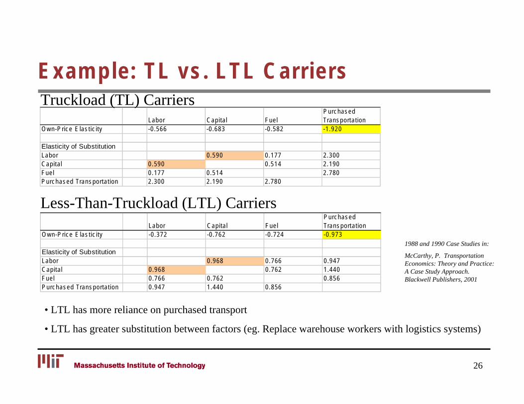
Example: TL vs. LTL Carriers

Labor Capital Fuel Purchased Transportation

Own-Price Elasticity -0.566 -0.683 -0.582 -1.920

Elasticity of Substitution Labor 0.590 0.177 2.300 Capital 0.590 0.514 2.190 Fuel 0.177 0.514 2.780 Purchased Transportation 2.300 2.190 2.780

Truckload (TL) Carriers

Less-Than-Truckload (LTL) Carriers

1988 and 1990 Case Studies in:

McCarthy, P. Transportation Economics: Theory and Practice: A Case Study Approach. Blackwell Publishers, 2001

Labor Capital Fuel Purchased Transportation

Own-Price Elasticity -0.372 -0.762 -0.724 -0.973

Elasticity of Substitution Labor 0.968 0.766 0.947 Capital 0.968 0.762 1.440 Fuel 0.766 0.762 0.856 Purchased Transportation 0.947 1.440 0.856

• LTL has more reliance on purchased transport

• LTL has greater substitution between factors (eg. Replace warehouse workers with logistics systems)

26

Outline

● Basic Concepts

● Production functions

● Profit maximization and cost minimization

● Average and marginal costs

27

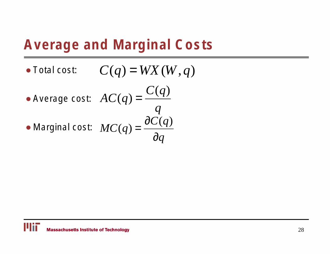
Average and Marginal Costs

● Total cost: C(q) = WX (W , q)

C(q) ● Average cost: AC (q) =

q∂C(q)

● Marginal cost: MC (q) = ∂q

28

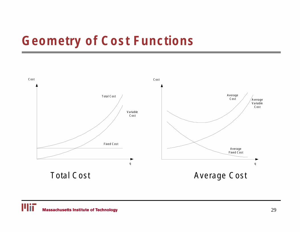
Geometry of Cost Functions

Cost Cost

q

Fixed Cost

Total Cost

Variable Cost

q

Average Fixed Cost

Average Cost Average

Variable Cost

Total Cost Average Cost

29

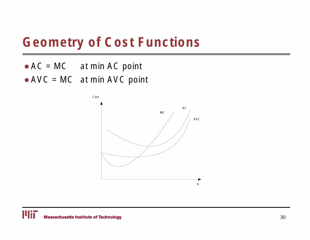
Geometry of Cost Functions

● AC = MC at min AC point

● AVC = MC at min AVC point

Cost

MC AC

AVC

q

30

Examples of Marginal Costs

● One additional passenger on a plane with empty seats – One extra meal

– Extra terminal possessing time

– Potential delays to other passengers

● 100 additional passengers/day to an air shuttle service – The costs above

– Extra flights

– Additional ground personnel

31

Using Average and Marginal Costs

● Profitability/Subsidy Requirements – Compare average cost and average revenue

● Profitability of a particular trip – Compare marginal cost and marginal revenue

● Economic efficiency – Price = MC

● Regulation – Declining average cost

32

Summary

● Basic Concepts ● Production functions

– Isoquants – Rate of technical substitution

● Profit maximization and cost minimization – Dual views of the same problem

● Average and marginal costs

Next lecture… Transportation costs

33

MIT OpenCourseWare http://ocw.mit.edu

1.201J / 11.545J / ESD.210J Transportation Systems Analysis: Demand and Economics Fall 2008

For information about citing these materials or our Terms of Use, visit: http://ocw.mit.edu/terms.