4B. Non-Keplerian Motion - LTAS-SDRG :: Welcome ! · 2017-10-26 · J.E. Prussing, B.A. Conway,...
123
Gaëtan Kerschen Space Structures & Systems Lab (S3L) 4B. Non-Keplerian Motion Astrodynamics (AERO0024)
-
Upload
truongtram -
Category
Documents
-
view
216 -
download
0
Transcript of 4B. Non-Keplerian Motion - LTAS-SDRG :: Welcome ! · 2017-10-26 · J.E. Prussing, B.A. Conway,...

Gaeumltan Kerschen
Space Structures amp
Systems Lab (S3L)
4B Non-Keplerian Motion
Astrodynamics (AERO0024)
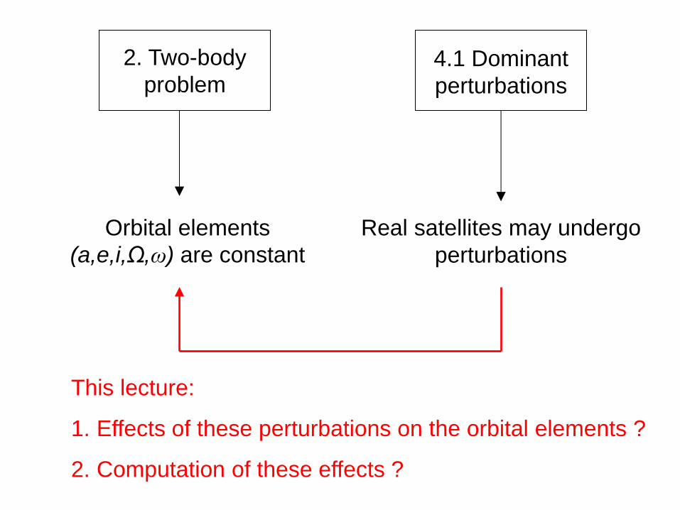
2 Two-body
problem 41 Dominant
perturbations
Orbital elements
(aeiΩω) are constant
Real satellites may undergo
perturbations
This lecture
1 Effects of these perturbations on the orbital elements
2 Computation of these effects
3
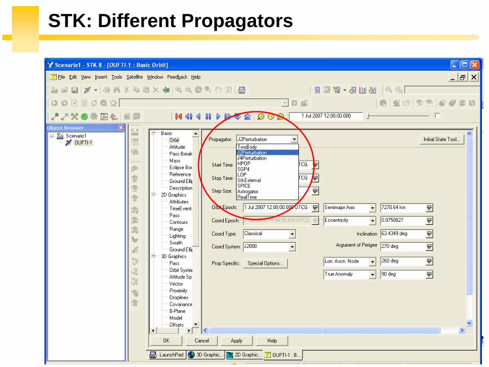
STK Different Propagators
4
Why Different Propagators
Analytic propagation
Better understanding of the perturbing forces
Useful for mission planning (fast answer) eg lifetime
computation
Numerical propagation
The high accuracy required today for satellite orbits can only be
achieved by using numerical integration
Incorporation of any arbitrary disturbing acceleration
(versatile)
5
4 Non-Keplerian Motion
2
2
(1 )
sin
sin 1 cos
a e
N
i e
42 Analytic treatment
43 Numerical methods
nt 1nt
r
44 Geostationary satellites
6
4 Non-Keplerian Motion
42 Analytic treatment
421 Variation of parameters
422 Non-spherical Earth
423 J2 propagator in STK
424 Atmospheric drag
425 Third-body perturbations
426 SGP4 propagator in STK
427 Solar radiation pressure
2
2
(1 )
sin
sin 1 cos
a e
N
i e
7
Analytic Treatment Definition
Position and velocity at a requested time are computed
directly from initial conditions in a single step
Analytic propagators use a closed-form solution of the
time-dependent motion of a satellite
Mainly used for the two dominant perturbations drag and
earth oblateness
42 Analytic treatment
8
Analytic Treatment Pros and Cons
Useful for mission planning and analysis (fast and insight)
Though the numerical integration methods can generate more
accurate ephemeris of a satellite with respect to a complex force
model the analytical solutions represent a manifold of solutions for
a large domain of initial conditions and parameters
But less accurate than numerical integration
Be aware of the assumptions made
42 Analytic treatment
9
Assumption for Analytic Developments
The magnitude of the disturbing force is assumed to be
much smaller than the magnitude of the attraction of the
satellite for the primary
3 perturbedr
r r a
perturbed a r
42 Analytic treatment
10
Variation of Parameters (VOP)
Originally developed by Euler and improved by Lagrange
(conservative) and Gauss (nonconservative)
It is called variation of parameters because the orbital
elements (ie the constant parameters in the two-body
equations) are changing in the presence of perturbations
The VOP equations are a system of first-order ODEs that
describe the rates of change of the orbital elements
421 Variation of parameters
a i e M
11
Disturbing Acceleration (Specific Force)
ˆ ˆ ˆRperturbed R T NT N a F e e e
2
421 Variation of parameters
Rotating basis whose
origin is fixed to the
satellite
12
Perturbation Equations (Gauss)
421 Variation of parameters
2a
Chapter 2
2
2
2
2
aa
2
h
r
2 2
2
1 sin sin
1 cos
h r e er r
e h h
(1)
(2)
(3)
The generating solution is that of the 2-body problem
ˆ ˆR Tr r rR r T Fr F e e (4)
Time rate-of-change
of the work done by
the disturbing force
13
Perturbation Equations (Gauss)
421 Variation of parameters
(1)
(2)
(3)
(4)
2 2 2
2
2 sin 2sin
2 sin 1 cos
a e h a ha R T e R T
h r h r
aRe T e
h
2(1 )h a e
3
22 sin 1 cos
1
aa Re T e
e
Chapter 2
14
Perturbation Equations (Gauss)
3
22 Resin 1 cos
1
aa T e
e
2(1 )
sin cos cosa e
e R T E
2
2cos(1 )
1 cos
Na ei
e
JE Prussing BA Conway Orbital Mechanics Oxford University Press
421 Variation of parameters
2 sin 2 cos1 (1 )cos cos
1 cos
T ea ei R
e e
2 2(1 ) 2 cos cos sin 2 cos with
1 cos
e R e e T eaM nt
e e
2
2sin(1 )
sin 1 cos
Na e
i e
15
Perturbation Equations (Gauss)
Limited to eccentricities less than 1
Singular for e=0 sin i=0 (use of equinoctial elements)
In what follows we apply the Gauss equations to Earth
oblateness and drag Analytical expressions for third-body
and solar radiation forces are far less common because
their effects are much smaller for many orbits
421 Variation of parameters
16
Non-spherical Earth J2
Focus on the oblateness through the first zonal harmonic
J2 (tesseral and sectorial coefficients ignored)
The J2 effect can still be viewed a small perturbation when
compared to the attraction of the spherical Earth
422 Non-spherical Earth
17
Disturbing Acceleration (Specific Force)
2 2 222
4
3 1 3sin sinsin sin cos sin sin cos
2r T N
J R ii i i
r
F e e e
422 Non-spherical Earth
2 2
2
3sin 11
2
satRU J
r r
1 1 ˆˆ ˆ with cos
Ur r r
F r φ λ
Chapter 4A
18
Physical Interpretation of the Perturbation
The oblateness means that the force of gravity is no longer
within the orbital plane non-planar motion will result
The equatorial bulge exerts a force that pulls the satellite
back to the equatorial plane and thus tries to align the
orbital plane with the equator
Due to its angular momentum the orbit behaves like a
spinning top and reacts with a precessional motion of the
orbital plane (the orbital plane of the satellite to rotate in
inertial space)
422 Non-spherical Earth
19
Physical Interpretation of the Perturbation
422 Non-spherical Earth
20
Effect of Perturbations on Orbital Elements
Secular rate of change average rate of change over many
orbits
Periodic rate of change rate of change within one orbit
(J2 ~ 8-10km with a period equal to the orbital period)
422 Non-spherical Earth
21
Effect of Perturbations on Orbital Elements
Periodic
Secular
422 Non-spherical Earth
22
Secular Effects on Orbital Elements
Nodal regression regression of the nodal line
Apsidal rotation rotation of the apse line
Mean anomaly
No secular variations for a e i
422 Non-spherical Earth
2
2
2 2 7 20
1 3cos
2 (1 )
T
avg
J Rdt i
T e a
2
22
2 2 7 20
1 34 5sin
4 (1 )
T
avg
J Rdt i
T e a
23
Secular Effects Node Line
2
2
2 2 7 20
1 3cos
2 (1 )
T
avg
J Rdt i
T e a
For posigrade orbits the node line drifts westward
(regression of the nodes) And conversely
0 90 0i
For polar orbits the node line is stationary
90 0i
422 Non-spherical Earth
Vallado Fundamental of
Astrodynamics and
Applications Kluwer 2001
25
Exploitation Sun-Synchronous Orbits
The orbital plane makes a constant angle with the radial
from the sun
422 Non-spherical Earth
26
Exploitation Sun-Synchronous Orbits
The orbital plane must rotate in inertial space with the
angular velocity of the Earth in its orbit around the Sun
360ordm per 36526 days or 09856ordm per day
The satellite sees any given swath of the planet under
nearly the same condition of daylight or darkness day after
day
422 Non-spherical Earth
27
Existing Satellites
SPOT-5
(820 kms 987ordm)
NOAAPOES
(833 kms 987ordm)
28
Secular Effects Apse Line
2
22
2 2 7 20
1 34 5sin
4 (1 )
T
avg
J Rdt i
T e a
The perigee advances in the direction of the motion
of the satellite And conversely
0 634 or 1166 180 0i i
The apse line does not move
634 or 1166 0i i
422 Non-spherical Earth
Vallado Fundamental of
Astrodynamics and
Applications Kluwer 2001
30
Exploitation Molniya Orbits
A geostationary satellite cannot view effectively the far
northern latitudes into which Russian territory extends
(+ costly plane change maneuver for the launch vehicle )
Molniya telecommunications satellites are launched from
Plesetsk (628ordmN) into 63ordm inclination orbits having a
period of 12 hours
3
2 the apse line is 53000km longellip
aT
422 Non-spherical Earth
31
Analytic Propagators in STK 2-body J2
2-body constant orbital elements
J2 accounts for secular variations in the orbit elements
due to Earth oblateness periodic variations are
neglected
423 J2 propagator in STK
32
J2 Propagator Underlying Equations
423 J2 propagator in STK
33
2-body and J2 Propagators Applied to ISS
Two-body propagator J2 propagator
423 J2 propagator in STK
34
HPOP and J2 Propagators Applied to ISS
Nodal regression of the ISS
35
Effects of Atmospheric Drag Semi-Major Axis
2a
Lecture 2
2
2
2
2
aa
gt0
Because drag causes the dissipation of mechanical energy
from the system the semimajor axis contracts
424 Atmospheric drag
Drag paradox the effect of atmospheric drag is to increase
the satellite speed and kinetic energy
36
Effects of Atmospheric Drag Semi-Major Axis
21 10
2 2D r D
A AN R T C v C
m m a
0D
Aa a C
m
2
Df i f i
C Aa a t t
m
is assumed constant
424 Atmospheric drag
3
22 Resin 1 cos
1
aa T e
e
Circular orbit
37
Effects of Atmospheric Drag Orbit Plane
2
2sin(1 )
sin 1 cos
Na e
i e
2
2cos(1 )
1 cos
Na ei
e
The orientation of the orbit plane is not changed by drag
424 Atmospheric drag
38
Effects of Atmospheric Drag Apogee Perigee
Apogee height changes drastically perigee height remains
relatively constant
424 Atmospheric drag
Vallado Fundamental of Astrodynamics and Applications Kluwer 2001
39
Effects of Atmospheric Drag Eccentricity
Vallado Fundamental of Astrodynamics and Applications Kluwer 2001
424 Atmospheric drag
40
Early Reentry of Skylab (1979)
Increased solar activity which
increased drag on Skylab led to
an early reentry
Earth reentry footprint could not
be accurately predicted (due to
tumbling and other parameters)
Debris was found around
Esperance (31ndash34degS 122ndash
126degE) The Shire of Esperance
fined the United States $400 for
littering a fine which to this day
remains unpaid
424 Atmospheric drag
41
Lost of ASCA Satellite (2000)
July 15 2000 a strong solar
flare heated the Earthrsquos
atmosphere increasing the
air density to a value 100
times greater than that for
which its ADCS had been
designed to cope The
magnetorquers were unable
to compensate and the
satellite was lost
httpheasarcgsfcnasagovdocsascasafemodehtml
424 Atmospheric drag
42
Effects of Third-Body Perturbations
The only secular perturbations are in the node and in the
perigee
For near-Earth orbits the dominance of the oblateness
dictates that the orbital plane regresses about the polar
axis For higher orbits the regression will be about some
mean pole lying between the Earthrsquos pole and the ecliptic
pole
Many geosynchronous satellites launched 30 years ago
now have inclinations of up to plusmn15ordm collision avoidance
as the satellites drift back through the GEO belt
425 Third-body perturbations
43
Effects of Third-Body Perturbations
Vallado Fundamental of Astrodynamics and Applications Kluwer 2001
The Sunrsquos attraction
tends to turn the
satellite ring into the
ecliptic The orbit
precesses about the
pole of the ecliptic
425 Third-body perturbations
44
STK Analytic Propagator (SGP4)
The J2 propagator does not include drag
SGP4 which stands for Simplified General Perturbations
Satellite Orbit Model 4 is a NASANORAD algorithm
426 SGP4 propagator in STK
45
STK Analytic Propagator (SGP4)
Several assumptions propagation valid for short durations
(3-10 days)
TLE data should be used as the input (see Lecture 03)
It considers secular and periodic variations due to Earth
oblateness solar and lunar gravitational effects and
orbital decay using a drag model
426 SGP4 propagator in STK
46
SGP4 Applied to ISS RAAN
426 SGP4 propagator in STK
47
SGP4 Applied to ISS Semi-Major Axis
426 SGP4 propagator in STK
48
Further Reading on the Web Site
426 SGP4 propagator in STK
49
Effects of Solar Radiation Pressure
The effects are usually small for most satellites
Satellites with very low mass and large surface area are
more affected
427 Solar radiation pressure
Vallado Fundamental of
Astrodynamics and
Applications Kluwer
2001
51
Secular Effects Orders of Magnitude
Vallado Fundamental of Astrodynamics and Applications Kluwer 2001
52
Periodic Effects Orders of Magnitude
Vallado Fundamental of Astrodynamics and Applications Kluwer 2001
53
4 Non-Keplerian Motion
2
2
(1 )
sin
sin 1 cos
a e
N
i e
43 Numerical methods
431 Orbit prediction
432 Numerical integration
433 Single-step methods Runge-Kutta
434 Multi-step methods
435 Integrator and step size selection
436 ISS example
nt 1nt
r
54
2-body analytic propagator (constant orbital elements)
J2 analytic propagator (secular variations in the orbit
elements due to Earth oblateness
HPOP numerical integration of the equations of motion
(periodic and secular effects included)
STK Propagators
431 Orbit prediction
Accurate
Versatile
Errors accumulation
for long intervals
Computationally
intensive
55
Real-Life Example German Aerospace Agency
431 Orbit prediction
56
Real-Life Example German Aerospace Agency
57
Further Reading on the Web Site
431 Orbit prediction
58
Real-Life Example Envisat
httpnngesocesadeenvisat
ENVpredhtml
431 Orbit prediction
Why do the
predictions degrade
for lower altitudes
60
NASA began the first complex numerical integrations
during the late 1960s and early 1970s
Did you Know
1969 1968
431 Orbit prediction
61
What is Numerical Integration
1n nt t t
3 perturbedr
r r a
Given
Compute
( ) ( )n nt tr r
1 1( ) ( )n nt t r r
432 Numerical integration
62
State-Space Formulation
3 perturbedr
r r a
( )f tu u
ru
r
6-dimensional
state vector
432 Numerical integration
63
How to Perform Numerical Integration
2( )( ) ( ) ( ) ( ) ( )
2
ss
n n n n n s
h hf t h f t hf t f t f t R
s
Taylor series expansion
( )ntu
1( )nt u
432 Numerical integration
64
First-Order Taylor Approximation (Euler)
1
( ) ( ) ( )
( )
n n n
n n n n
t t t t t
t f t
u u u
u u uEuler step
0 1 2 3 4 5 60
5
10
15
20
25
30
35
40
Time t (s)
x(t
)=t2
Exact solution
The stepsize has to be extremely
small for accurate predictions
and it is necessary to develop
more effective algorithms
along the tangent
432 Numerical integration
65
Numerical Integration Methods
1 1 1
1 0
m m
n j n j j n j
j j
t
u u u
0 0
Implicit the solution method becomes
iterative in the nonlinear case
0 0 Explicit un+1 can be deduced directly from
the results at the previous time steps
=0
for 1
j j
j
Single-step the system at time tn+1
only depends on the previous state tn
State vector
0
for 1
j j
j
Multi-step the system at time tn+1 depends
several previous states tntn-1etc
432 Numerical integration
66
Examples Implicit vs Explicit
Trapezoidal rule (implicit)
nt 1nt
Euler forward (explicit)
nt 1nt
Euler backward (implicit)
nt 1nt
1n n nt u u u
1 1n n nt u u u
1
12
n n
n n t
u uu u
r
r
r
432 Numerical integration
67
A variety of methods has been applied in astrodynamics
Each of these methods has its own advantages and
drawbacks
Accuracy what is the order of the integration scheme
Efficiency how many function calls
Versatility can it be applied to a wide range of problems
Complexity is it easy to implement and use
Step size automatic step size control
Why Different Methods
431 Orbit prediction
68
Runge-Kutta Family Single-Step
Perhaps the most well-known numerical integrator
Difference with traditional Taylor series integrators the RK
family only requires the first derivative but several
evaluations are needed to move forward one step in time
Different variants explicit embedded etc
433 Single-step methods Runge-Kutta
69
Runge-Kutta Family Single-Step
with ( ) ( )t f tu u 0 0( )t u u
1
1
s
n n i i
i
t b
u u k
1 1
1
1
2
n n
i
i n ij j n i
j
f t c t
f t a t c t i s
k u
k u k
Slopes at
various points
within the
integration step
433 Single-step methods Runge-Kutta
70
Runge-Kutta Family Single-Step
Butcher Tableau
The Runge-Kutta methods are fully described by the
coefficients
c1
c2
cs
a21
as1
b1
as2
b2
ass-1
bs-1 hellip
hellip
hellip hellip hellip
bs
1
1
1
1
1
0
s
i
i
i
i ij
j
b
c
c a
433 Single-step methods Runge-Kutta
71
RK4 (Explicit)
1 2 3 41
2 2
6n n t
k k k ku u
Butcher Tableau
1
2 1
3 2
4 3
2 2
2 2
n n
n n
n n
n n
f t
t tf t
t tf t
f t t t
k u
k u k
k u k
k u k
433 Single-step methods Runge-Kutta
72
RK4 (Explicit)
1 2 3 41
2 2
6n n t
k k k ku u
1
2 1
3 2
4 3
2 2
2 2
n n
n n
n n
n n
f t
t tf t
t tf t
f t t t
k u
k u k
k u k
k u k
Slope at the beginning
Slope at the midpoint (k1 is
used to determine the value
of u Euler)
Slope at the midpoint (k2 is
now used)
Slope at the end
Estimated slope
(weighted average)
433 Single-step methods Runge-Kutta
73
RK4 (Explicit)
nt 2nt t nt t
1k3k
2k
4k
Estimate at new
time
u
433 Single-step methods Runge-Kutta
74
RK4 (Explicit)
The local truncation error for a 4th order RK is O(h5)
The accuracy is comparable to that of a 4th order Taylor
series but the Runge-Kutta method avoids the
calculation of higher-order derivatives
Easy to use and implement
The step size is fixed
433 Single-step methods Runge-Kutta
75
RK4 in STK
433 Single-step methods Runge-Kutta
76
Embedded Methods
They produce an estimate of the local truncation error
adjust the step size to keep local truncation errors
within some tolerances
This is done by having two methods in the tableau one with
order p and one with order p+1 with the same set of
function evaluations
( 1) ( 1) ( 1)
1
1
sp p p
n n i i
i
t b
u u k
( ) ( ) ( )
1
1
sp p p
n n i i
i
t b
u u k
433 Single-step methods Runge-Kutta
77
Embedded Methods
The two different approximations for the solution at each
step are compared
If the two answers are in close agreement the approximation is
accepted
If the two answers do not agree to a specified accuracy the step
size is reduced
If the answers agree to more significant digits than required the
step size is increased
433 Single-step methods Runge-Kutta
78
Ode45 in Matlab Simulink
Runge-Kutta (45) pair of Dormand and Prince
Variable step size
Matlab help This should be the first solver you try
433 Single-step methods Runge-Kutta
79
Ode45 in Matlab Simulink
edit ode45
433 Single-step methods Runge-Kutta
80
Ode45 in Matlab Simulink
Be very careful with the default parameters
options = odeset(RelTol1e-8AbsTol1e-8)
433 Single-step methods Runge-Kutta
81
RKF 7(8) Default Method in STK
Runge-Kutta-Fehlberg integration method of 7th order
with 8th order error control for the integration step size
433 Single-step methods Runge-Kutta
83
Multi-Step Methods (Predictor-Corrector)
They estimate the state over time using previously
determined back values of the solution
Unlike RK methods they only perform one evaluation for
each step forward but they usually have a predictor and a
corrector formula
Adams() ndash Bashforth - Moulton Gauss - Jackson
() The first with Le Verrier to predict the existence and position of Neptune
434 Multi-step methods
84
Multi-Step Methods Principle
( ) ( )t f tu u1
1( ) ( ) ( ) n
n
t
n nt
t t f t dt
u u u
unknown
Replace it by a
polynomial that
interpolates the
previous values Four function values
interpolated by a
third-order polynomial
t
u
434 Multi-step methods
85
Multi-Step Methods Initiation
with ( ) ( )t f tu u 0 0( )t u u
What is the inherent problem
t
u
434 Multi-step methods
86
Multi-Step Methods Initiation
Because these methods require back values they are not
self-starting
One may for instance use of a single-step method to
compute the first four values
434 Multi-step methods
87
Gauss-Jackson in STK
One of the most recommendable fixed-stepsize multistep
methods for orbit computations
88
Integrator Selection
435 Integrator and step size selection
Montenbruck and Gill
Satellite orbits Springer
2000
89
Integrator Selection
Pros
Very fast
Cons
Special starting procedure
Fixed time steps
Error control
Pros
Plug and play
Error control
Cons
Slower
Multi-step Single step
435 Integrator and step size selection
90
Why is the Step Size So Critical
Theoretical arguments
1 The accuracy and the stability of the algorithm are
directly related to the step size
2 Nonlinear equations of motion
Data for Landsat 4 and 6 in circular orbits around 800km
indicates that a one-minute step size yields about 47m
error
A three-minute step size produces about a 900m error
435 Integrator and step size selection
91
Why is the Step Size So Critical
More practical arguments
1 The computation time is directly related to the
step size
2 The particular choice of step size depends on the
most rapidly varying component in the disturbing
functions (eg 50 x 50 gravity field)
435 Integrator and step size selection
92
Appropriate Step Size
The problem of determining an appropriate step size is a
challenge in any numerical process
Fixed step size (rule of thumb for standard
applications)
But an algorithm with variable step size is really
helpful The step size is chosen in such a way that
each step contributes uniformly to the total integration
error
100
orbitTt
435 Integrator and step size selection
93
Three Examples XMM OUFTI-1 ISS
Can you plot the step size vs true anomaly
435 Integrator and step size selection
94
XMM Report in STK
435 Integrator and step size selection
95
XMM (e~08)
0 50 100 150 200 250 300 350 4000
1000
2000
3000
4000
5000
6000
True anomaly (deg)
Ste
p s
ize
(s)
435 Integrator and step size selection
96
ISS(e~0)
435 Integrator and step size selection
0 50 100 150 200 250 300 350 40030
35
40
45
50
55
60
65
70
True anomaly (deg)
Ste
p s
ize
(s)
97
ldquoDifficultrdquo Orbits
Automatic time step is especially nice on highly eccentric
orbits (Molniya XMM) These orbits are best computed
using variable step sizes to maintain some given level of
accuracy
Without this variable step size we waste a lot of time near
apoapsis when the integration is taking too small a step
Likewise the integrator may not be using a small enough step
size at periapsis where the satellite is traveling fast
435 Integrator and step size selection
98
HPOP Propagator ISS Example
1 Earthrsquos oblateness only
2 Drag only
3 Sun and moon only
4 SRP only
5 All together
436 ISS example
99
Earthrsquos Oblateness Only Ω
HPOP
J2
2-body
436 ISS example
100
Earthrsquos Oblateness Only i Ω a
HPOP with central body (20 + WGS84_EGM96)
(without dragSRPSun and Moon)
436 ISS example
101
Drag Only i Ω a
HPOP with drag ndash Harris Priester
(without oblatenessSRPSun and Moon)
436 ISS example
102
Drag Relationship with Eclipses
103
SRP Only i Ω a
HPOP with SRP
(without oblatenessdragSun and Moon)
436 ISS example
104
SRP Relationship with Eclipses
105
All Perturbations Together
436 ISS example
106
4 Non-Keplerian Motion
2
2
(1 )
sin
sin 1 cos
a e
N
i e
44 Geostationary satellites
107
Practical Example GEO Satellites
Nice illustration of
1 Perturbations of the 2-body problem
2 Secular and periodic contributions
3 Accuracy required by practical applications
4 The need for orbit correction and thrust forces
And it is a real-life example (telecommunications
meteorology)
44 GEO satellites
108
Three Main Perturbations for GEO Satellites
44 GEO satellites
1 Non-spherical Earth
2 SRP
3 Sun and Moon
109
Station Keeping of GEO Satellites
The effect of the perturbations is to cause the spacecraft
to drift away from its nominal station If the drift was
allowed to build up unchecked the spacecraft could
become useless
A station-keeping box is defined by a longitude and a
maximum authorized distance for satellite excursions in
longitude and latitude
For instance TC2 -8ordm plusmn 007ordm EW plusmn 005ordm NS
44 GEO satellites
110
East-West and North-South Drift
44 GEO satellites
NS drift
EW drift
What are the perturbations generating these drifts
111
East-West Drift
44 GEO satellites
A GEO satellite drifts in longitude due to the influence of
two main perturbations
1 The elliptic nature of the Earthrsquos equatorial cross-
section J22 (and not from the NS oblateness J2)
2
ΔV
ΔV vsat
vsat SRP
112
East-West Drift due to Equatorial Ellipticity
44 GEO satellites
113
East-West Drift due to Equatorial Ellipticity
44 GEO satellites
114
East-West Drift HPOP (20) vs HPOP (22)
44 GEO satellites
115
East-West Drift Stable Equilibirum
HPOP with 22
(without Sun and moonSRPdrag)
116
East-West Drift Stable Equilibirum
HPOP with 22
(without Sun and moonSRPdrag)
117
East-West Drift Stable Equilibirum
HPOP with 22
(without Sun and moonSRPdrag)
118
North-South Drift
The perturbations caused by the Sun and the Moon are
predominantly out-of-plane effects causing a change in
the inclination and in the right ascension of the orbit
ascending node
Similar effects on the orbit to those of the Earthrsquos
oblateness (but here with respect to the ecliptic)
A GEO satellite therefore drifts in latitude with a
fundamental period equal to the orbit period
119
North-South Drift
Period
HPOP with Sun and Moon
(without oblatenessSRPdrag)
120
North-South Drift
Period
HPOP with Sun and Moon
(without oblatenessSRPdrag)
121
Thrust Forces for Stationkeeping
GEO spacecraft require continual stationkeeping to stay
within the authorized box using onboard thrusters
44 GEO satellites
122
42 ANALYTIC TREATMENT
421 Variation of parameters
422 Non-spherical Earth
423 J2 propagator in STK
424 Atmospheric drag
425 Third-body perturbations
426 SGP4 propagator in STK
427 Solar radiation pressure
4 Non-Keplerian Motion
43 NUMERICAL METHODS
431 Orbit prediction
432 Numerical integration
433 Single-step methods Runge-Kutta
434 Multi-step methods
435 Integrator and step size selection
436 ISS example
44 GEOSTATIONARY SATELLITES
Gaeumltan Kerschen
Space Structures amp
Systems Lab (S3L)
4B Non-Keplerian Motion
Astrodynamics (AERO0024)
2 Two-body
problem 41 Dominant
perturbations
Orbital elements
(aeiΩω) are constant
Real satellites may undergo
perturbations
This lecture
1 Effects of these perturbations on the orbital elements
2 Computation of these effects
3
STK Different Propagators
4
Why Different Propagators
Analytic propagation
Better understanding of the perturbing forces
Useful for mission planning (fast answer) eg lifetime
computation
Numerical propagation
The high accuracy required today for satellite orbits can only be
achieved by using numerical integration
Incorporation of any arbitrary disturbing acceleration
(versatile)
5
4 Non-Keplerian Motion
2
2
(1 )
sin
sin 1 cos
a e
N
i e
42 Analytic treatment
43 Numerical methods
nt 1nt
r
44 Geostationary satellites
6
4 Non-Keplerian Motion
42 Analytic treatment
421 Variation of parameters
422 Non-spherical Earth
423 J2 propagator in STK
424 Atmospheric drag
425 Third-body perturbations
426 SGP4 propagator in STK
427 Solar radiation pressure
2
2
(1 )
sin
sin 1 cos
a e
N
i e
7
Analytic Treatment Definition
Position and velocity at a requested time are computed
directly from initial conditions in a single step
Analytic propagators use a closed-form solution of the
time-dependent motion of a satellite
Mainly used for the two dominant perturbations drag and
earth oblateness
42 Analytic treatment
8
Analytic Treatment Pros and Cons
Useful for mission planning and analysis (fast and insight)
Though the numerical integration methods can generate more
accurate ephemeris of a satellite with respect to a complex force
model the analytical solutions represent a manifold of solutions for
a large domain of initial conditions and parameters
But less accurate than numerical integration
Be aware of the assumptions made
42 Analytic treatment
9
Assumption for Analytic Developments
The magnitude of the disturbing force is assumed to be
much smaller than the magnitude of the attraction of the
satellite for the primary
3 perturbedr
r r a
perturbed a r
42 Analytic treatment
10
Variation of Parameters (VOP)
Originally developed by Euler and improved by Lagrange
(conservative) and Gauss (nonconservative)
It is called variation of parameters because the orbital
elements (ie the constant parameters in the two-body
equations) are changing in the presence of perturbations
The VOP equations are a system of first-order ODEs that
describe the rates of change of the orbital elements
421 Variation of parameters
a i e M
11
Disturbing Acceleration (Specific Force)
ˆ ˆ ˆRperturbed R T NT N a F e e e
2
421 Variation of parameters
Rotating basis whose
origin is fixed to the
satellite
12
Perturbation Equations (Gauss)
421 Variation of parameters
2a
Chapter 2
2
2
2
2
aa
2
h
r
2 2
2
1 sin sin
1 cos
h r e er r
e h h
(1)
(2)
(3)
The generating solution is that of the 2-body problem
ˆ ˆR Tr r rR r T Fr F e e (4)
Time rate-of-change
of the work done by
the disturbing force
13
Perturbation Equations (Gauss)
421 Variation of parameters
(1)
(2)
(3)
(4)
2 2 2
2
2 sin 2sin
2 sin 1 cos
a e h a ha R T e R T
h r h r
aRe T e
h
2(1 )h a e
3
22 sin 1 cos
1
aa Re T e
e
Chapter 2
14
Perturbation Equations (Gauss)
3
22 Resin 1 cos
1
aa T e
e
2(1 )
sin cos cosa e
e R T E
2
2cos(1 )
1 cos
Na ei
e
JE Prussing BA Conway Orbital Mechanics Oxford University Press
421 Variation of parameters
2 sin 2 cos1 (1 )cos cos
1 cos
T ea ei R
e e
2 2(1 ) 2 cos cos sin 2 cos with
1 cos
e R e e T eaM nt
e e
2
2sin(1 )
sin 1 cos
Na e
i e
15
Perturbation Equations (Gauss)
Limited to eccentricities less than 1
Singular for e=0 sin i=0 (use of equinoctial elements)
In what follows we apply the Gauss equations to Earth
oblateness and drag Analytical expressions for third-body
and solar radiation forces are far less common because
their effects are much smaller for many orbits
421 Variation of parameters
16
Non-spherical Earth J2
Focus on the oblateness through the first zonal harmonic
J2 (tesseral and sectorial coefficients ignored)
The J2 effect can still be viewed a small perturbation when
compared to the attraction of the spherical Earth
422 Non-spherical Earth
17
Disturbing Acceleration (Specific Force)
2 2 222
4
3 1 3sin sinsin sin cos sin sin cos
2r T N
J R ii i i
r
F e e e
422 Non-spherical Earth
2 2
2
3sin 11
2
satRU J
r r
1 1 ˆˆ ˆ with cos
Ur r r
F r φ λ
Chapter 4A
18
Physical Interpretation of the Perturbation
The oblateness means that the force of gravity is no longer
within the orbital plane non-planar motion will result
The equatorial bulge exerts a force that pulls the satellite
back to the equatorial plane and thus tries to align the
orbital plane with the equator
Due to its angular momentum the orbit behaves like a
spinning top and reacts with a precessional motion of the
orbital plane (the orbital plane of the satellite to rotate in
inertial space)
422 Non-spherical Earth
19
Physical Interpretation of the Perturbation
422 Non-spherical Earth
20
Effect of Perturbations on Orbital Elements
Secular rate of change average rate of change over many
orbits
Periodic rate of change rate of change within one orbit
(J2 ~ 8-10km with a period equal to the orbital period)
422 Non-spherical Earth
21
Effect of Perturbations on Orbital Elements
Periodic
Secular
422 Non-spherical Earth
22
Secular Effects on Orbital Elements
Nodal regression regression of the nodal line
Apsidal rotation rotation of the apse line
Mean anomaly
No secular variations for a e i
422 Non-spherical Earth
2
2
2 2 7 20
1 3cos
2 (1 )
T
avg
J Rdt i
T e a
2
22
2 2 7 20
1 34 5sin
4 (1 )
T
avg
J Rdt i
T e a
23
Secular Effects Node Line
2
2
2 2 7 20
1 3cos
2 (1 )
T
avg
J Rdt i
T e a
For posigrade orbits the node line drifts westward
(regression of the nodes) And conversely
0 90 0i
For polar orbits the node line is stationary
90 0i
422 Non-spherical Earth
Vallado Fundamental of
Astrodynamics and
Applications Kluwer 2001
25
Exploitation Sun-Synchronous Orbits
The orbital plane makes a constant angle with the radial
from the sun
422 Non-spherical Earth
26
Exploitation Sun-Synchronous Orbits
The orbital plane must rotate in inertial space with the
angular velocity of the Earth in its orbit around the Sun
360ordm per 36526 days or 09856ordm per day
The satellite sees any given swath of the planet under
nearly the same condition of daylight or darkness day after
day
422 Non-spherical Earth
27
Existing Satellites
SPOT-5
(820 kms 987ordm)
NOAAPOES
(833 kms 987ordm)
28
Secular Effects Apse Line
2
22
2 2 7 20
1 34 5sin
4 (1 )
T
avg
J Rdt i
T e a
The perigee advances in the direction of the motion
of the satellite And conversely
0 634 or 1166 180 0i i
The apse line does not move
634 or 1166 0i i
422 Non-spherical Earth
Vallado Fundamental of
Astrodynamics and
Applications Kluwer 2001
30
Exploitation Molniya Orbits
A geostationary satellite cannot view effectively the far
northern latitudes into which Russian territory extends
(+ costly plane change maneuver for the launch vehicle )
Molniya telecommunications satellites are launched from
Plesetsk (628ordmN) into 63ordm inclination orbits having a
period of 12 hours
3
2 the apse line is 53000km longellip
aT
422 Non-spherical Earth
31
Analytic Propagators in STK 2-body J2
2-body constant orbital elements
J2 accounts for secular variations in the orbit elements
due to Earth oblateness periodic variations are
neglected
423 J2 propagator in STK
32
J2 Propagator Underlying Equations
423 J2 propagator in STK
33
2-body and J2 Propagators Applied to ISS
Two-body propagator J2 propagator
423 J2 propagator in STK
34
HPOP and J2 Propagators Applied to ISS
Nodal regression of the ISS
35
Effects of Atmospheric Drag Semi-Major Axis
2a
Lecture 2
2
2
2
2
aa
gt0
Because drag causes the dissipation of mechanical energy
from the system the semimajor axis contracts
424 Atmospheric drag
Drag paradox the effect of atmospheric drag is to increase
the satellite speed and kinetic energy
36
Effects of Atmospheric Drag Semi-Major Axis
21 10
2 2D r D
A AN R T C v C
m m a
0D
Aa a C
m
2
Df i f i
C Aa a t t
m
is assumed constant
424 Atmospheric drag
3
22 Resin 1 cos
1
aa T e
e
Circular orbit
37
Effects of Atmospheric Drag Orbit Plane
2
2sin(1 )
sin 1 cos
Na e
i e
2
2cos(1 )
1 cos
Na ei
e
The orientation of the orbit plane is not changed by drag
424 Atmospheric drag
38
Effects of Atmospheric Drag Apogee Perigee
Apogee height changes drastically perigee height remains
relatively constant
424 Atmospheric drag
Vallado Fundamental of Astrodynamics and Applications Kluwer 2001
39
Effects of Atmospheric Drag Eccentricity
Vallado Fundamental of Astrodynamics and Applications Kluwer 2001
424 Atmospheric drag
40
Early Reentry of Skylab (1979)
Increased solar activity which
increased drag on Skylab led to
an early reentry
Earth reentry footprint could not
be accurately predicted (due to
tumbling and other parameters)
Debris was found around
Esperance (31ndash34degS 122ndash
126degE) The Shire of Esperance
fined the United States $400 for
littering a fine which to this day
remains unpaid
424 Atmospheric drag
41
Lost of ASCA Satellite (2000)
July 15 2000 a strong solar
flare heated the Earthrsquos
atmosphere increasing the
air density to a value 100
times greater than that for
which its ADCS had been
designed to cope The
magnetorquers were unable
to compensate and the
satellite was lost
httpheasarcgsfcnasagovdocsascasafemodehtml
424 Atmospheric drag
42
Effects of Third-Body Perturbations
The only secular perturbations are in the node and in the
perigee
For near-Earth orbits the dominance of the oblateness
dictates that the orbital plane regresses about the polar
axis For higher orbits the regression will be about some
mean pole lying between the Earthrsquos pole and the ecliptic
pole
Many geosynchronous satellites launched 30 years ago
now have inclinations of up to plusmn15ordm collision avoidance
as the satellites drift back through the GEO belt
425 Third-body perturbations
43
Effects of Third-Body Perturbations
Vallado Fundamental of Astrodynamics and Applications Kluwer 2001
The Sunrsquos attraction
tends to turn the
satellite ring into the
ecliptic The orbit
precesses about the
pole of the ecliptic
425 Third-body perturbations
44
STK Analytic Propagator (SGP4)
The J2 propagator does not include drag
SGP4 which stands for Simplified General Perturbations
Satellite Orbit Model 4 is a NASANORAD algorithm
426 SGP4 propagator in STK
45
STK Analytic Propagator (SGP4)
Several assumptions propagation valid for short durations
(3-10 days)
TLE data should be used as the input (see Lecture 03)
It considers secular and periodic variations due to Earth
oblateness solar and lunar gravitational effects and
orbital decay using a drag model
426 SGP4 propagator in STK
46
SGP4 Applied to ISS RAAN
426 SGP4 propagator in STK
47
SGP4 Applied to ISS Semi-Major Axis
426 SGP4 propagator in STK
48
Further Reading on the Web Site
426 SGP4 propagator in STK
49
Effects of Solar Radiation Pressure
The effects are usually small for most satellites
Satellites with very low mass and large surface area are
more affected
427 Solar radiation pressure
Vallado Fundamental of
Astrodynamics and
Applications Kluwer
2001
51
Secular Effects Orders of Magnitude
Vallado Fundamental of Astrodynamics and Applications Kluwer 2001
52
Periodic Effects Orders of Magnitude
Vallado Fundamental of Astrodynamics and Applications Kluwer 2001
53
4 Non-Keplerian Motion
2
2
(1 )
sin
sin 1 cos
a e
N
i e
43 Numerical methods
431 Orbit prediction
432 Numerical integration
433 Single-step methods Runge-Kutta
434 Multi-step methods
435 Integrator and step size selection
436 ISS example
nt 1nt
r
54
2-body analytic propagator (constant orbital elements)
J2 analytic propagator (secular variations in the orbit
elements due to Earth oblateness
HPOP numerical integration of the equations of motion
(periodic and secular effects included)
STK Propagators
431 Orbit prediction
Accurate
Versatile
Errors accumulation
for long intervals
Computationally
intensive
55
Real-Life Example German Aerospace Agency
431 Orbit prediction
56
Real-Life Example German Aerospace Agency
57
Further Reading on the Web Site
431 Orbit prediction
58
Real-Life Example Envisat
httpnngesocesadeenvisat
ENVpredhtml
431 Orbit prediction
Why do the
predictions degrade
for lower altitudes
60
NASA began the first complex numerical integrations
during the late 1960s and early 1970s
Did you Know
1969 1968
431 Orbit prediction
61
What is Numerical Integration
1n nt t t
3 perturbedr
r r a
Given
Compute
( ) ( )n nt tr r
1 1( ) ( )n nt t r r
432 Numerical integration
62
State-Space Formulation
3 perturbedr
r r a
( )f tu u
ru
r
6-dimensional
state vector
432 Numerical integration
63
How to Perform Numerical Integration
2( )( ) ( ) ( ) ( ) ( )
2
ss
n n n n n s
h hf t h f t hf t f t f t R
s
Taylor series expansion
( )ntu
1( )nt u
432 Numerical integration
64
First-Order Taylor Approximation (Euler)
1
( ) ( ) ( )
( )
n n n
n n n n
t t t t t
t f t
u u u
u u uEuler step
0 1 2 3 4 5 60
5
10
15
20
25
30
35
40
Time t (s)
x(t
)=t2
Exact solution
The stepsize has to be extremely
small for accurate predictions
and it is necessary to develop
more effective algorithms
along the tangent
432 Numerical integration
65
Numerical Integration Methods
1 1 1
1 0
m m
n j n j j n j
j j
t
u u u
0 0
Implicit the solution method becomes
iterative in the nonlinear case
0 0 Explicit un+1 can be deduced directly from
the results at the previous time steps
=0
for 1
j j
j
Single-step the system at time tn+1
only depends on the previous state tn
State vector
0
for 1
j j
j
Multi-step the system at time tn+1 depends
several previous states tntn-1etc
432 Numerical integration
66
Examples Implicit vs Explicit
Trapezoidal rule (implicit)
nt 1nt
Euler forward (explicit)
nt 1nt
Euler backward (implicit)
nt 1nt
1n n nt u u u
1 1n n nt u u u
1
12
n n
n n t
u uu u
r
r
r
432 Numerical integration
67
A variety of methods has been applied in astrodynamics
Each of these methods has its own advantages and
drawbacks
Accuracy what is the order of the integration scheme
Efficiency how many function calls
Versatility can it be applied to a wide range of problems
Complexity is it easy to implement and use
Step size automatic step size control
Why Different Methods
431 Orbit prediction
68
Runge-Kutta Family Single-Step
Perhaps the most well-known numerical integrator
Difference with traditional Taylor series integrators the RK
family only requires the first derivative but several
evaluations are needed to move forward one step in time
Different variants explicit embedded etc
433 Single-step methods Runge-Kutta
69
Runge-Kutta Family Single-Step
with ( ) ( )t f tu u 0 0( )t u u
1
1
s
n n i i
i
t b
u u k
1 1
1
1
2
n n
i
i n ij j n i
j
f t c t
f t a t c t i s
k u
k u k
Slopes at
various points
within the
integration step
433 Single-step methods Runge-Kutta
70
Runge-Kutta Family Single-Step
Butcher Tableau
The Runge-Kutta methods are fully described by the
coefficients
c1
c2
cs
a21
as1
b1
as2
b2
ass-1
bs-1 hellip
hellip
hellip hellip hellip
bs
1
1
1
1
1
0
s
i
i
i
i ij
j
b
c
c a
433 Single-step methods Runge-Kutta
71
RK4 (Explicit)
1 2 3 41
2 2
6n n t
k k k ku u
Butcher Tableau
1
2 1
3 2
4 3
2 2
2 2
n n
n n
n n
n n
f t
t tf t
t tf t
f t t t
k u
k u k
k u k
k u k
433 Single-step methods Runge-Kutta
72
RK4 (Explicit)
1 2 3 41
2 2
6n n t
k k k ku u
1
2 1
3 2
4 3
2 2
2 2
n n
n n
n n
n n
f t
t tf t
t tf t
f t t t
k u
k u k
k u k
k u k
Slope at the beginning
Slope at the midpoint (k1 is
used to determine the value
of u Euler)
Slope at the midpoint (k2 is
now used)
Slope at the end
Estimated slope
(weighted average)
433 Single-step methods Runge-Kutta
73
RK4 (Explicit)
nt 2nt t nt t
1k3k
2k
4k
Estimate at new
time
u
433 Single-step methods Runge-Kutta
74
RK4 (Explicit)
The local truncation error for a 4th order RK is O(h5)
The accuracy is comparable to that of a 4th order Taylor
series but the Runge-Kutta method avoids the
calculation of higher-order derivatives
Easy to use and implement
The step size is fixed
433 Single-step methods Runge-Kutta
75
RK4 in STK
433 Single-step methods Runge-Kutta
76
Embedded Methods
They produce an estimate of the local truncation error
adjust the step size to keep local truncation errors
within some tolerances
This is done by having two methods in the tableau one with
order p and one with order p+1 with the same set of
function evaluations
( 1) ( 1) ( 1)
1
1
sp p p
n n i i
i
t b
u u k
( ) ( ) ( )
1
1
sp p p
n n i i
i
t b
u u k
433 Single-step methods Runge-Kutta
77
Embedded Methods
The two different approximations for the solution at each
step are compared
If the two answers are in close agreement the approximation is
accepted
If the two answers do not agree to a specified accuracy the step
size is reduced
If the answers agree to more significant digits than required the
step size is increased
433 Single-step methods Runge-Kutta
78
Ode45 in Matlab Simulink
Runge-Kutta (45) pair of Dormand and Prince
Variable step size
Matlab help This should be the first solver you try
433 Single-step methods Runge-Kutta
79
Ode45 in Matlab Simulink
edit ode45
433 Single-step methods Runge-Kutta
80
Ode45 in Matlab Simulink
Be very careful with the default parameters
options = odeset(RelTol1e-8AbsTol1e-8)
433 Single-step methods Runge-Kutta
81
RKF 7(8) Default Method in STK
Runge-Kutta-Fehlberg integration method of 7th order
with 8th order error control for the integration step size
433 Single-step methods Runge-Kutta
83
Multi-Step Methods (Predictor-Corrector)
They estimate the state over time using previously
determined back values of the solution
Unlike RK methods they only perform one evaluation for
each step forward but they usually have a predictor and a
corrector formula
Adams() ndash Bashforth - Moulton Gauss - Jackson
() The first with Le Verrier to predict the existence and position of Neptune
434 Multi-step methods
84
Multi-Step Methods Principle
( ) ( )t f tu u1
1( ) ( ) ( ) n
n
t
n nt
t t f t dt
u u u
unknown
Replace it by a
polynomial that
interpolates the
previous values Four function values
interpolated by a
third-order polynomial
t
u
434 Multi-step methods
85
Multi-Step Methods Initiation
with ( ) ( )t f tu u 0 0( )t u u
What is the inherent problem
t
u
434 Multi-step methods
86
Multi-Step Methods Initiation
Because these methods require back values they are not
self-starting
One may for instance use of a single-step method to
compute the first four values
434 Multi-step methods
87
Gauss-Jackson in STK
One of the most recommendable fixed-stepsize multistep
methods for orbit computations
88
Integrator Selection
435 Integrator and step size selection
Montenbruck and Gill
Satellite orbits Springer
2000
89
Integrator Selection
Pros
Very fast
Cons
Special starting procedure
Fixed time steps
Error control
Pros
Plug and play
Error control
Cons
Slower
Multi-step Single step
435 Integrator and step size selection
90
Why is the Step Size So Critical
Theoretical arguments
1 The accuracy and the stability of the algorithm are
directly related to the step size
2 Nonlinear equations of motion
Data for Landsat 4 and 6 in circular orbits around 800km
indicates that a one-minute step size yields about 47m
error
A three-minute step size produces about a 900m error
435 Integrator and step size selection
91
Why is the Step Size So Critical
More practical arguments
1 The computation time is directly related to the
step size
2 The particular choice of step size depends on the
most rapidly varying component in the disturbing
functions (eg 50 x 50 gravity field)
435 Integrator and step size selection
92
Appropriate Step Size
The problem of determining an appropriate step size is a
challenge in any numerical process
Fixed step size (rule of thumb for standard
applications)
But an algorithm with variable step size is really
helpful The step size is chosen in such a way that
each step contributes uniformly to the total integration
error
100
orbitTt
435 Integrator and step size selection
93
Three Examples XMM OUFTI-1 ISS
Can you plot the step size vs true anomaly
435 Integrator and step size selection
94
XMM Report in STK
435 Integrator and step size selection
95
XMM (e~08)
0 50 100 150 200 250 300 350 4000
1000
2000
3000
4000
5000
6000
True anomaly (deg)
Ste
p s
ize
(s)
435 Integrator and step size selection
96
ISS(e~0)
435 Integrator and step size selection
0 50 100 150 200 250 300 350 40030
35
40
45
50
55
60
65
70
True anomaly (deg)
Ste
p s
ize
(s)
97
ldquoDifficultrdquo Orbits
Automatic time step is especially nice on highly eccentric
orbits (Molniya XMM) These orbits are best computed
using variable step sizes to maintain some given level of
accuracy
Without this variable step size we waste a lot of time near
apoapsis when the integration is taking too small a step
Likewise the integrator may not be using a small enough step
size at periapsis where the satellite is traveling fast
435 Integrator and step size selection
98
HPOP Propagator ISS Example
1 Earthrsquos oblateness only
2 Drag only
3 Sun and moon only
4 SRP only
5 All together
436 ISS example
99
Earthrsquos Oblateness Only Ω
HPOP
J2
2-body
436 ISS example
100
Earthrsquos Oblateness Only i Ω a
HPOP with central body (20 + WGS84_EGM96)
(without dragSRPSun and Moon)
436 ISS example
101
Drag Only i Ω a
HPOP with drag ndash Harris Priester
(without oblatenessSRPSun and Moon)
436 ISS example
102
Drag Relationship with Eclipses
103
SRP Only i Ω a
HPOP with SRP
(without oblatenessdragSun and Moon)
436 ISS example
104
SRP Relationship with Eclipses
105
All Perturbations Together
436 ISS example
106
4 Non-Keplerian Motion
2
2
(1 )
sin
sin 1 cos
a e
N
i e
44 Geostationary satellites
107
Practical Example GEO Satellites
Nice illustration of
1 Perturbations of the 2-body problem
2 Secular and periodic contributions
3 Accuracy required by practical applications
4 The need for orbit correction and thrust forces
And it is a real-life example (telecommunications
meteorology)
44 GEO satellites
108
Three Main Perturbations for GEO Satellites
44 GEO satellites
1 Non-spherical Earth
2 SRP
3 Sun and Moon
109
Station Keeping of GEO Satellites
The effect of the perturbations is to cause the spacecraft
to drift away from its nominal station If the drift was
allowed to build up unchecked the spacecraft could
become useless
A station-keeping box is defined by a longitude and a
maximum authorized distance for satellite excursions in
longitude and latitude
For instance TC2 -8ordm plusmn 007ordm EW plusmn 005ordm NS
44 GEO satellites
110
East-West and North-South Drift
44 GEO satellites
NS drift
EW drift
What are the perturbations generating these drifts
111
East-West Drift
44 GEO satellites
A GEO satellite drifts in longitude due to the influence of
two main perturbations
1 The elliptic nature of the Earthrsquos equatorial cross-
section J22 (and not from the NS oblateness J2)
2
ΔV
ΔV vsat
vsat SRP
112
East-West Drift due to Equatorial Ellipticity
44 GEO satellites
113
East-West Drift due to Equatorial Ellipticity
44 GEO satellites
114
East-West Drift HPOP (20) vs HPOP (22)
44 GEO satellites
115
East-West Drift Stable Equilibirum
HPOP with 22
(without Sun and moonSRPdrag)
116
East-West Drift Stable Equilibirum
HPOP with 22
(without Sun and moonSRPdrag)
117
East-West Drift Stable Equilibirum
HPOP with 22
(without Sun and moonSRPdrag)
118
North-South Drift
The perturbations caused by the Sun and the Moon are
predominantly out-of-plane effects causing a change in
the inclination and in the right ascension of the orbit
ascending node
Similar effects on the orbit to those of the Earthrsquos
oblateness (but here with respect to the ecliptic)
A GEO satellite therefore drifts in latitude with a
fundamental period equal to the orbit period
119
North-South Drift
Period
HPOP with Sun and Moon
(without oblatenessSRPdrag)
120
North-South Drift
Period
HPOP with Sun and Moon
(without oblatenessSRPdrag)
121
Thrust Forces for Stationkeeping
GEO spacecraft require continual stationkeeping to stay
within the authorized box using onboard thrusters
44 GEO satellites
122
42 ANALYTIC TREATMENT
421 Variation of parameters
422 Non-spherical Earth
423 J2 propagator in STK
424 Atmospheric drag
425 Third-body perturbations
426 SGP4 propagator in STK
427 Solar radiation pressure
4 Non-Keplerian Motion
43 NUMERICAL METHODS
431 Orbit prediction
432 Numerical integration
433 Single-step methods Runge-Kutta
434 Multi-step methods
435 Integrator and step size selection
436 ISS example
44 GEOSTATIONARY SATELLITES
Gaeumltan Kerschen
Space Structures amp
Systems Lab (S3L)
4B Non-Keplerian Motion
Astrodynamics (AERO0024)
3
STK Different Propagators
4
Why Different Propagators
Analytic propagation
Better understanding of the perturbing forces
Useful for mission planning (fast answer) eg lifetime
computation
Numerical propagation
The high accuracy required today for satellite orbits can only be
achieved by using numerical integration
Incorporation of any arbitrary disturbing acceleration
(versatile)
5
4 Non-Keplerian Motion
2
2
(1 )
sin
sin 1 cos
a e
N
i e
42 Analytic treatment
43 Numerical methods
nt 1nt
r
44 Geostationary satellites
6
4 Non-Keplerian Motion
42 Analytic treatment
421 Variation of parameters
422 Non-spherical Earth
423 J2 propagator in STK
424 Atmospheric drag
425 Third-body perturbations
426 SGP4 propagator in STK
427 Solar radiation pressure
2
2
(1 )
sin
sin 1 cos
a e
N
i e
7
Analytic Treatment Definition
Position and velocity at a requested time are computed
directly from initial conditions in a single step
Analytic propagators use a closed-form solution of the
time-dependent motion of a satellite
Mainly used for the two dominant perturbations drag and
earth oblateness
42 Analytic treatment
8
Analytic Treatment Pros and Cons
Useful for mission planning and analysis (fast and insight)
Though the numerical integration methods can generate more
accurate ephemeris of a satellite with respect to a complex force
model the analytical solutions represent a manifold of solutions for
a large domain of initial conditions and parameters
But less accurate than numerical integration
Be aware of the assumptions made
42 Analytic treatment
9
Assumption for Analytic Developments
The magnitude of the disturbing force is assumed to be
much smaller than the magnitude of the attraction of the
satellite for the primary
3 perturbedr
r r a
perturbed a r
42 Analytic treatment
10
Variation of Parameters (VOP)
Originally developed by Euler and improved by Lagrange
(conservative) and Gauss (nonconservative)
It is called variation of parameters because the orbital
elements (ie the constant parameters in the two-body
equations) are changing in the presence of perturbations
The VOP equations are a system of first-order ODEs that
describe the rates of change of the orbital elements
421 Variation of parameters
a i e M
11
Disturbing Acceleration (Specific Force)
ˆ ˆ ˆRperturbed R T NT N a F e e e
2
421 Variation of parameters
Rotating basis whose
origin is fixed to the
satellite
12
Perturbation Equations (Gauss)
421 Variation of parameters
2a
Chapter 2
2
2
2
2
aa
2
h
r
2 2
2
1 sin sin
1 cos
h r e er r
e h h
(1)
(2)
(3)
The generating solution is that of the 2-body problem
ˆ ˆR Tr r rR r T Fr F e e (4)
Time rate-of-change
of the work done by
the disturbing force
13
Perturbation Equations (Gauss)
421 Variation of parameters
(1)
(2)
(3)
(4)
2 2 2
2
2 sin 2sin
2 sin 1 cos
a e h a ha R T e R T
h r h r
aRe T e
h
2(1 )h a e
3
22 sin 1 cos
1
aa Re T e
e
Chapter 2
14
Perturbation Equations (Gauss)
3
22 Resin 1 cos
1
aa T e
e
2(1 )
sin cos cosa e
e R T E
2
2cos(1 )
1 cos
Na ei
e
JE Prussing BA Conway Orbital Mechanics Oxford University Press
421 Variation of parameters
2 sin 2 cos1 (1 )cos cos
1 cos
T ea ei R
e e
2 2(1 ) 2 cos cos sin 2 cos with
1 cos
e R e e T eaM nt
e e
2
2sin(1 )
sin 1 cos
Na e
i e
15
Perturbation Equations (Gauss)
Limited to eccentricities less than 1
Singular for e=0 sin i=0 (use of equinoctial elements)
In what follows we apply the Gauss equations to Earth
oblateness and drag Analytical expressions for third-body
and solar radiation forces are far less common because
their effects are much smaller for many orbits
421 Variation of parameters
16
Non-spherical Earth J2
Focus on the oblateness through the first zonal harmonic
J2 (tesseral and sectorial coefficients ignored)
The J2 effect can still be viewed a small perturbation when
compared to the attraction of the spherical Earth
422 Non-spherical Earth
17
Disturbing Acceleration (Specific Force)
2 2 222
4
3 1 3sin sinsin sin cos sin sin cos
2r T N
J R ii i i
r
F e e e
422 Non-spherical Earth
2 2
2
3sin 11
2
satRU J
r r
1 1 ˆˆ ˆ with cos
Ur r r
F r φ λ
Chapter 4A
18
Physical Interpretation of the Perturbation
The oblateness means that the force of gravity is no longer
within the orbital plane non-planar motion will result
The equatorial bulge exerts a force that pulls the satellite
back to the equatorial plane and thus tries to align the
orbital plane with the equator
Due to its angular momentum the orbit behaves like a
spinning top and reacts with a precessional motion of the
orbital plane (the orbital plane of the satellite to rotate in
inertial space)
422 Non-spherical Earth
19
Physical Interpretation of the Perturbation
422 Non-spherical Earth
20
Effect of Perturbations on Orbital Elements
Secular rate of change average rate of change over many
orbits
Periodic rate of change rate of change within one orbit
(J2 ~ 8-10km with a period equal to the orbital period)
422 Non-spherical Earth
21
Effect of Perturbations on Orbital Elements
Periodic
Secular
422 Non-spherical Earth
22
Secular Effects on Orbital Elements
Nodal regression regression of the nodal line
Apsidal rotation rotation of the apse line
Mean anomaly
No secular variations for a e i
422 Non-spherical Earth
2
2
2 2 7 20
1 3cos
2 (1 )
T
avg
J Rdt i
T e a
2
22
2 2 7 20
1 34 5sin
4 (1 )
T
avg
J Rdt i
T e a
23
Secular Effects Node Line
2
2
2 2 7 20
1 3cos
2 (1 )
T
avg
J Rdt i
T e a
For posigrade orbits the node line drifts westward
(regression of the nodes) And conversely
0 90 0i
For polar orbits the node line is stationary
90 0i
422 Non-spherical Earth
Vallado Fundamental of
Astrodynamics and
Applications Kluwer 2001
25
Exploitation Sun-Synchronous Orbits
The orbital plane makes a constant angle with the radial
from the sun
422 Non-spherical Earth
26
Exploitation Sun-Synchronous Orbits
The orbital plane must rotate in inertial space with the
angular velocity of the Earth in its orbit around the Sun
360ordm per 36526 days or 09856ordm per day
The satellite sees any given swath of the planet under
nearly the same condition of daylight or darkness day after
day
422 Non-spherical Earth
27
Existing Satellites
SPOT-5
(820 kms 987ordm)
NOAAPOES
(833 kms 987ordm)
28
Secular Effects Apse Line
2
22
2 2 7 20
1 34 5sin
4 (1 )
T
avg
J Rdt i
T e a
The perigee advances in the direction of the motion
of the satellite And conversely
0 634 or 1166 180 0i i
The apse line does not move
634 or 1166 0i i
422 Non-spherical Earth
Vallado Fundamental of
Astrodynamics and
Applications Kluwer 2001
30
Exploitation Molniya Orbits
A geostationary satellite cannot view effectively the far
northern latitudes into which Russian territory extends
(+ costly plane change maneuver for the launch vehicle )
Molniya telecommunications satellites are launched from
Plesetsk (628ordmN) into 63ordm inclination orbits having a
period of 12 hours
3
2 the apse line is 53000km longellip
aT
422 Non-spherical Earth
31
Analytic Propagators in STK 2-body J2
2-body constant orbital elements
J2 accounts for secular variations in the orbit elements
due to Earth oblateness periodic variations are
neglected
423 J2 propagator in STK
32
J2 Propagator Underlying Equations
423 J2 propagator in STK
33
2-body and J2 Propagators Applied to ISS
Two-body propagator J2 propagator
423 J2 propagator in STK
34
HPOP and J2 Propagators Applied to ISS
Nodal regression of the ISS
35
Effects of Atmospheric Drag Semi-Major Axis
2a
Lecture 2
2
2
2
2
aa
gt0
Because drag causes the dissipation of mechanical energy
from the system the semimajor axis contracts
424 Atmospheric drag
Drag paradox the effect of atmospheric drag is to increase
the satellite speed and kinetic energy
36
Effects of Atmospheric Drag Semi-Major Axis
21 10
2 2D r D
A AN R T C v C
m m a
0D
Aa a C
m
2
Df i f i
C Aa a t t
m
is assumed constant
424 Atmospheric drag
3
22 Resin 1 cos
1
aa T e
e
Circular orbit
37
Effects of Atmospheric Drag Orbit Plane
2
2sin(1 )
sin 1 cos
Na e
i e
2
2cos(1 )
1 cos
Na ei
e
The orientation of the orbit plane is not changed by drag
424 Atmospheric drag
38
Effects of Atmospheric Drag Apogee Perigee
Apogee height changes drastically perigee height remains
relatively constant
424 Atmospheric drag
Vallado Fundamental of Astrodynamics and Applications Kluwer 2001
39
Effects of Atmospheric Drag Eccentricity
Vallado Fundamental of Astrodynamics and Applications Kluwer 2001
424 Atmospheric drag
40
Early Reentry of Skylab (1979)
Increased solar activity which
increased drag on Skylab led to
an early reentry
Earth reentry footprint could not
be accurately predicted (due to
tumbling and other parameters)
Debris was found around
Esperance (31ndash34degS 122ndash
126degE) The Shire of Esperance
fined the United States $400 for
littering a fine which to this day
remains unpaid
424 Atmospheric drag
41
Lost of ASCA Satellite (2000)
July 15 2000 a strong solar
flare heated the Earthrsquos
atmosphere increasing the
air density to a value 100
times greater than that for
which its ADCS had been
designed to cope The
magnetorquers were unable
to compensate and the
satellite was lost
httpheasarcgsfcnasagovdocsascasafemodehtml
424 Atmospheric drag
42
Effects of Third-Body Perturbations
The only secular perturbations are in the node and in the
perigee
For near-Earth orbits the dominance of the oblateness
dictates that the orbital plane regresses about the polar
axis For higher orbits the regression will be about some
mean pole lying between the Earthrsquos pole and the ecliptic
pole
Many geosynchronous satellites launched 30 years ago
now have inclinations of up to plusmn15ordm collision avoidance
as the satellites drift back through the GEO belt
425 Third-body perturbations
43
Effects of Third-Body Perturbations
Vallado Fundamental of Astrodynamics and Applications Kluwer 2001
The Sunrsquos attraction
tends to turn the
satellite ring into the
ecliptic The orbit
precesses about the
pole of the ecliptic
425 Third-body perturbations
44
STK Analytic Propagator (SGP4)
The J2 propagator does not include drag
SGP4 which stands for Simplified General Perturbations
Satellite Orbit Model 4 is a NASANORAD algorithm
426 SGP4 propagator in STK
45
STK Analytic Propagator (SGP4)
Several assumptions propagation valid for short durations
(3-10 days)
TLE data should be used as the input (see Lecture 03)
It considers secular and periodic variations due to Earth
oblateness solar and lunar gravitational effects and
orbital decay using a drag model
426 SGP4 propagator in STK
46
SGP4 Applied to ISS RAAN
426 SGP4 propagator in STK
47
SGP4 Applied to ISS Semi-Major Axis
426 SGP4 propagator in STK
48
Further Reading on the Web Site
426 SGP4 propagator in STK
49
Effects of Solar Radiation Pressure
The effects are usually small for most satellites
Satellites with very low mass and large surface area are
more affected
427 Solar radiation pressure
Vallado Fundamental of
Astrodynamics and
Applications Kluwer
2001
51
Secular Effects Orders of Magnitude
Vallado Fundamental of Astrodynamics and Applications Kluwer 2001
52
Periodic Effects Orders of Magnitude
Vallado Fundamental of Astrodynamics and Applications Kluwer 2001
53
4 Non-Keplerian Motion
2
2
(1 )
sin
sin 1 cos
a e
N
i e
43 Numerical methods
431 Orbit prediction
432 Numerical integration
433 Single-step methods Runge-Kutta
434 Multi-step methods
435 Integrator and step size selection
436 ISS example
nt 1nt
r
54
2-body analytic propagator (constant orbital elements)
J2 analytic propagator (secular variations in the orbit
elements due to Earth oblateness
HPOP numerical integration of the equations of motion
(periodic and secular effects included)
STK Propagators
431 Orbit prediction
Accurate
Versatile
Errors accumulation
for long intervals
Computationally
intensive
55
Real-Life Example German Aerospace Agency
431 Orbit prediction
56
Real-Life Example German Aerospace Agency
57
Further Reading on the Web Site
431 Orbit prediction
58
Real-Life Example Envisat
httpnngesocesadeenvisat
ENVpredhtml
431 Orbit prediction
Why do the
predictions degrade
for lower altitudes
60
NASA began the first complex numerical integrations
during the late 1960s and early 1970s
Did you Know
1969 1968
431 Orbit prediction
61
What is Numerical Integration
1n nt t t
3 perturbedr
r r a
Given
Compute
( ) ( )n nt tr r
1 1( ) ( )n nt t r r
432 Numerical integration
62
State-Space Formulation
3 perturbedr
r r a
( )f tu u
ru
r
6-dimensional
state vector
432 Numerical integration
63
How to Perform Numerical Integration
2( )( ) ( ) ( ) ( ) ( )
2
ss
n n n n n s
h hf t h f t hf t f t f t R
s
Taylor series expansion
( )ntu
1( )nt u
432 Numerical integration
64
First-Order Taylor Approximation (Euler)
1
( ) ( ) ( )
( )
n n n
n n n n
t t t t t
t f t
u u u
u u uEuler step
0 1 2 3 4 5 60
5
10
15
20
25
30
35
40
Time t (s)
x(t
)=t2
Exact solution
The stepsize has to be extremely
small for accurate predictions
and it is necessary to develop
more effective algorithms
along the tangent
432 Numerical integration
65
Numerical Integration Methods
1 1 1
1 0
m m
n j n j j n j
j j
t
u u u
0 0
Implicit the solution method becomes
iterative in the nonlinear case
0 0 Explicit un+1 can be deduced directly from
the results at the previous time steps
=0
for 1
j j
j
Single-step the system at time tn+1
only depends on the previous state tn
State vector
0
for 1
j j
j
Multi-step the system at time tn+1 depends
several previous states tntn-1etc
432 Numerical integration
66
Examples Implicit vs Explicit
Trapezoidal rule (implicit)
nt 1nt
Euler forward (explicit)
nt 1nt
Euler backward (implicit)
nt 1nt
1n n nt u u u
1 1n n nt u u u
1
12
n n
n n t
u uu u
r
r
r
432 Numerical integration
67
A variety of methods has been applied in astrodynamics
Each of these methods has its own advantages and
drawbacks
Accuracy what is the order of the integration scheme
Efficiency how many function calls
Versatility can it be applied to a wide range of problems
Complexity is it easy to implement and use
Step size automatic step size control
Why Different Methods
431 Orbit prediction
68
Runge-Kutta Family Single-Step
Perhaps the most well-known numerical integrator
Difference with traditional Taylor series integrators the RK
family only requires the first derivative but several
evaluations are needed to move forward one step in time
Different variants explicit embedded etc
433 Single-step methods Runge-Kutta
69
Runge-Kutta Family Single-Step
with ( ) ( )t f tu u 0 0( )t u u
1
1
s
n n i i
i
t b
u u k
1 1
1
1
2
n n
i
i n ij j n i
j
f t c t
f t a t c t i s
k u
k u k
Slopes at
various points
within the
integration step
433 Single-step methods Runge-Kutta
70
Runge-Kutta Family Single-Step
Butcher Tableau
The Runge-Kutta methods are fully described by the
coefficients
c1
c2
cs
a21
as1
b1
as2
b2
ass-1
bs-1 hellip
hellip
hellip hellip hellip
bs
1
1
1
1
1
0
s
i
i
i
i ij
j
b
c
c a
433 Single-step methods Runge-Kutta
71
RK4 (Explicit)
1 2 3 41
2 2
6n n t
k k k ku u
Butcher Tableau
1
2 1
3 2
4 3
2 2
2 2
n n
n n
n n
n n
f t
t tf t
t tf t
f t t t
k u
k u k
k u k
k u k
433 Single-step methods Runge-Kutta
72
RK4 (Explicit)
1 2 3 41
2 2
6n n t
k k k ku u
1
2 1
3 2
4 3
2 2
2 2
n n
n n
n n
n n
f t
t tf t
t tf t
f t t t
k u
k u k
k u k
k u k
Slope at the beginning
Slope at the midpoint (k1 is
used to determine the value
of u Euler)
Slope at the midpoint (k2 is
now used)
Slope at the end
Estimated slope
(weighted average)
433 Single-step methods Runge-Kutta
73
RK4 (Explicit)
nt 2nt t nt t
1k3k
2k
4k
Estimate at new
time
u
433 Single-step methods Runge-Kutta
74
RK4 (Explicit)
The local truncation error for a 4th order RK is O(h5)
The accuracy is comparable to that of a 4th order Taylor
series but the Runge-Kutta method avoids the
calculation of higher-order derivatives
Easy to use and implement
The step size is fixed
433 Single-step methods Runge-Kutta
75
RK4 in STK
433 Single-step methods Runge-Kutta
76
Embedded Methods
They produce an estimate of the local truncation error
adjust the step size to keep local truncation errors
within some tolerances
This is done by having two methods in the tableau one with
order p and one with order p+1 with the same set of
function evaluations
( 1) ( 1) ( 1)
1
1
sp p p
n n i i
i
t b
u u k
( ) ( ) ( )
1
1
sp p p
n n i i
i
t b
u u k
433 Single-step methods Runge-Kutta
77
Embedded Methods
The two different approximations for the solution at each
step are compared
If the two answers are in close agreement the approximation is
accepted
If the two answers do not agree to a specified accuracy the step
size is reduced
If the answers agree to more significant digits than required the
step size is increased
433 Single-step methods Runge-Kutta
78
Ode45 in Matlab Simulink
Runge-Kutta (45) pair of Dormand and Prince
Variable step size
Matlab help This should be the first solver you try
433 Single-step methods Runge-Kutta
79
Ode45 in Matlab Simulink
edit ode45
433 Single-step methods Runge-Kutta
80
Ode45 in Matlab Simulink
Be very careful with the default parameters
options = odeset(RelTol1e-8AbsTol1e-8)
433 Single-step methods Runge-Kutta
81
RKF 7(8) Default Method in STK
Runge-Kutta-Fehlberg integration method of 7th order
with 8th order error control for the integration step size
433 Single-step methods Runge-Kutta
83
Multi-Step Methods (Predictor-Corrector)
They estimate the state over time using previously
determined back values of the solution
Unlike RK methods they only perform one evaluation for
each step forward but they usually have a predictor and a
corrector formula
Adams() ndash Bashforth - Moulton Gauss - Jackson
() The first with Le Verrier to predict the existence and position of Neptune
434 Multi-step methods
84
Multi-Step Methods Principle
( ) ( )t f tu u1
1( ) ( ) ( ) n
n
t
n nt
t t f t dt
u u u
unknown
Replace it by a
polynomial that
interpolates the
previous values Four function values
interpolated by a
third-order polynomial
t
u
434 Multi-step methods
85
Multi-Step Methods Initiation
with ( ) ( )t f tu u 0 0( )t u u
What is the inherent problem
t
u
434 Multi-step methods
86
Multi-Step Methods Initiation
Because these methods require back values they are not
self-starting
One may for instance use of a single-step method to
compute the first four values
434 Multi-step methods
87
Gauss-Jackson in STK
One of the most recommendable fixed-stepsize multistep
methods for orbit computations
88
Integrator Selection
435 Integrator and step size selection
Montenbruck and Gill
Satellite orbits Springer
2000
89
Integrator Selection
Pros
Very fast
Cons
Special starting procedure
Fixed time steps
Error control
Pros
Plug and play
Error control
Cons
Slower
Multi-step Single step
435 Integrator and step size selection
90
Why is the Step Size So Critical
Theoretical arguments
1 The accuracy and the stability of the algorithm are
directly related to the step size
2 Nonlinear equations of motion
Data for Landsat 4 and 6 in circular orbits around 800km
indicates that a one-minute step size yields about 47m
error
A three-minute step size produces about a 900m error
435 Integrator and step size selection
91
Why is the Step Size So Critical
More practical arguments
1 The computation time is directly related to the
step size
2 The particular choice of step size depends on the
most rapidly varying component in the disturbing
functions (eg 50 x 50 gravity field)
435 Integrator and step size selection
92
Appropriate Step Size
The problem of determining an appropriate step size is a
challenge in any numerical process
Fixed step size (rule of thumb for standard
applications)
But an algorithm with variable step size is really
helpful The step size is chosen in such a way that
each step contributes uniformly to the total integration
error
100
orbitTt
435 Integrator and step size selection
93
Three Examples XMM OUFTI-1 ISS
Can you plot the step size vs true anomaly
435 Integrator and step size selection
94
XMM Report in STK
435 Integrator and step size selection
95
XMM (e~08)
0 50 100 150 200 250 300 350 4000
1000
2000
3000
4000
5000
6000
True anomaly (deg)
Ste
p s
ize
(s)
435 Integrator and step size selection
96
ISS(e~0)
435 Integrator and step size selection
0 50 100 150 200 250 300 350 40030
35
40
45
50
55
60
65
70
True anomaly (deg)
Ste
p s
ize
(s)
97
ldquoDifficultrdquo Orbits
Automatic time step is especially nice on highly eccentric
orbits (Molniya XMM) These orbits are best computed
using variable step sizes to maintain some given level of
accuracy
Without this variable step size we waste a lot of time near
apoapsis when the integration is taking too small a step
Likewise the integrator may not be using a small enough step
size at periapsis where the satellite is traveling fast
435 Integrator and step size selection
98
HPOP Propagator ISS Example
1 Earthrsquos oblateness only
2 Drag only
3 Sun and moon only
4 SRP only
5 All together
436 ISS example
99
Earthrsquos Oblateness Only Ω
HPOP
J2
2-body
436 ISS example
100
Earthrsquos Oblateness Only i Ω a
HPOP with central body (20 + WGS84_EGM96)
(without dragSRPSun and Moon)
436 ISS example
101
Drag Only i Ω a
HPOP with drag ndash Harris Priester
(without oblatenessSRPSun and Moon)
436 ISS example
102
Drag Relationship with Eclipses
103
SRP Only i Ω a
HPOP with SRP
(without oblatenessdragSun and Moon)
436 ISS example
104
SRP Relationship with Eclipses
105
All Perturbations Together
436 ISS example
106
4 Non-Keplerian Motion
2
2
(1 )
sin
sin 1 cos
a e
N
i e
44 Geostationary satellites
107
Practical Example GEO Satellites
Nice illustration of
1 Perturbations of the 2-body problem
2 Secular and periodic contributions
3 Accuracy required by practical applications
4 The need for orbit correction and thrust forces
And it is a real-life example (telecommunications
meteorology)
44 GEO satellites
108
Three Main Perturbations for GEO Satellites
44 GEO satellites
1 Non-spherical Earth
2 SRP
3 Sun and Moon
109
Station Keeping of GEO Satellites
The effect of the perturbations is to cause the spacecraft
to drift away from its nominal station If the drift was
allowed to build up unchecked the spacecraft could
become useless
A station-keeping box is defined by a longitude and a
maximum authorized distance for satellite excursions in
longitude and latitude
For instance TC2 -8ordm plusmn 007ordm EW plusmn 005ordm NS
44 GEO satellites
110
East-West and North-South Drift
44 GEO satellites
NS drift
EW drift
What are the perturbations generating these drifts
111
East-West Drift
44 GEO satellites
A GEO satellite drifts in longitude due to the influence of
two main perturbations
1 The elliptic nature of the Earthrsquos equatorial cross-
section J22 (and not from the NS oblateness J2)
2
ΔV
ΔV vsat
vsat SRP
112
East-West Drift due to Equatorial Ellipticity
44 GEO satellites
113
East-West Drift due to Equatorial Ellipticity
44 GEO satellites
114
East-West Drift HPOP (20) vs HPOP (22)
44 GEO satellites
115
East-West Drift Stable Equilibirum
HPOP with 22
(without Sun and moonSRPdrag)
116
East-West Drift Stable Equilibirum
HPOP with 22
(without Sun and moonSRPdrag)
117
East-West Drift Stable Equilibirum
HPOP with 22
(without Sun and moonSRPdrag)
118
North-South Drift
The perturbations caused by the Sun and the Moon are
predominantly out-of-plane effects causing a change in
the inclination and in the right ascension of the orbit
ascending node
Similar effects on the orbit to those of the Earthrsquos
oblateness (but here with respect to the ecliptic)
A GEO satellite therefore drifts in latitude with a
fundamental period equal to the orbit period
119
North-South Drift
Period
HPOP with Sun and Moon
(without oblatenessSRPdrag)
120
North-South Drift
Period
HPOP with Sun and Moon
(without oblatenessSRPdrag)
121
Thrust Forces for Stationkeeping
GEO spacecraft require continual stationkeeping to stay
within the authorized box using onboard thrusters
44 GEO satellites
122
42 ANALYTIC TREATMENT
421 Variation of parameters
422 Non-spherical Earth
423 J2 propagator in STK
424 Atmospheric drag
425 Third-body perturbations
426 SGP4 propagator in STK
427 Solar radiation pressure
4 Non-Keplerian Motion
43 NUMERICAL METHODS
431 Orbit prediction
432 Numerical integration
433 Single-step methods Runge-Kutta
434 Multi-step methods
435 Integrator and step size selection
436 ISS example
44 GEOSTATIONARY SATELLITES
Gaeumltan Kerschen
Space Structures amp
Systems Lab (S3L)
4B Non-Keplerian Motion
Astrodynamics (AERO0024)
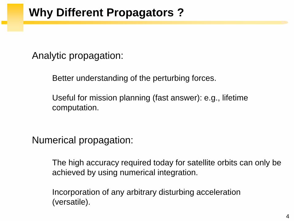
4
Why Different Propagators
Analytic propagation
Better understanding of the perturbing forces
Useful for mission planning (fast answer) eg lifetime
computation
Numerical propagation
The high accuracy required today for satellite orbits can only be
achieved by using numerical integration
Incorporation of any arbitrary disturbing acceleration
(versatile)
5
4 Non-Keplerian Motion
2
2
(1 )
sin
sin 1 cos
a e
N
i e
42 Analytic treatment
43 Numerical methods
nt 1nt
r
44 Geostationary satellites
6
4 Non-Keplerian Motion
42 Analytic treatment
421 Variation of parameters
422 Non-spherical Earth
423 J2 propagator in STK
424 Atmospheric drag
425 Third-body perturbations
426 SGP4 propagator in STK
427 Solar radiation pressure
2
2
(1 )
sin
sin 1 cos
a e
N
i e
7
Analytic Treatment Definition
Position and velocity at a requested time are computed
directly from initial conditions in a single step
Analytic propagators use a closed-form solution of the
time-dependent motion of a satellite
Mainly used for the two dominant perturbations drag and
earth oblateness
42 Analytic treatment
8
Analytic Treatment Pros and Cons
Useful for mission planning and analysis (fast and insight)
Though the numerical integration methods can generate more
accurate ephemeris of a satellite with respect to a complex force
model the analytical solutions represent a manifold of solutions for
a large domain of initial conditions and parameters
But less accurate than numerical integration
Be aware of the assumptions made
42 Analytic treatment
9
Assumption for Analytic Developments
The magnitude of the disturbing force is assumed to be
much smaller than the magnitude of the attraction of the
satellite for the primary
3 perturbedr
r r a
perturbed a r
42 Analytic treatment
10
Variation of Parameters (VOP)
Originally developed by Euler and improved by Lagrange
(conservative) and Gauss (nonconservative)
It is called variation of parameters because the orbital
elements (ie the constant parameters in the two-body
equations) are changing in the presence of perturbations
The VOP equations are a system of first-order ODEs that
describe the rates of change of the orbital elements
421 Variation of parameters
a i e M
11
Disturbing Acceleration (Specific Force)
ˆ ˆ ˆRperturbed R T NT N a F e e e
2
421 Variation of parameters
Rotating basis whose
origin is fixed to the
satellite
12
Perturbation Equations (Gauss)
421 Variation of parameters
2a
Chapter 2
2
2
2
2
aa
2
h
r
2 2
2
1 sin sin
1 cos
h r e er r
e h h
(1)
(2)
(3)
The generating solution is that of the 2-body problem
ˆ ˆR Tr r rR r T Fr F e e (4)
Time rate-of-change
of the work done by
the disturbing force
13
Perturbation Equations (Gauss)
421 Variation of parameters
(1)
(2)
(3)
(4)
2 2 2
2
2 sin 2sin
2 sin 1 cos
a e h a ha R T e R T
h r h r
aRe T e
h
2(1 )h a e
3
22 sin 1 cos
1
aa Re T e
e
Chapter 2
14
Perturbation Equations (Gauss)
3
22 Resin 1 cos
1
aa T e
e
2(1 )
sin cos cosa e
e R T E
2
2cos(1 )
1 cos
Na ei
e
JE Prussing BA Conway Orbital Mechanics Oxford University Press
421 Variation of parameters
2 sin 2 cos1 (1 )cos cos
1 cos
T ea ei R
e e
2 2(1 ) 2 cos cos sin 2 cos with
1 cos
e R e e T eaM nt
e e
2
2sin(1 )
sin 1 cos
Na e
i e
15
Perturbation Equations (Gauss)
Limited to eccentricities less than 1
Singular for e=0 sin i=0 (use of equinoctial elements)
In what follows we apply the Gauss equations to Earth
oblateness and drag Analytical expressions for third-body
and solar radiation forces are far less common because
their effects are much smaller for many orbits
421 Variation of parameters
16
Non-spherical Earth J2
Focus on the oblateness through the first zonal harmonic
J2 (tesseral and sectorial coefficients ignored)
The J2 effect can still be viewed a small perturbation when
compared to the attraction of the spherical Earth
422 Non-spherical Earth
17
Disturbing Acceleration (Specific Force)
2 2 222
4
3 1 3sin sinsin sin cos sin sin cos
2r T N
J R ii i i
r
F e e e
422 Non-spherical Earth
2 2
2
3sin 11
2
satRU J
r r
1 1 ˆˆ ˆ with cos
Ur r r
F r φ λ
Chapter 4A
18
Physical Interpretation of the Perturbation
The oblateness means that the force of gravity is no longer
within the orbital plane non-planar motion will result
The equatorial bulge exerts a force that pulls the satellite
back to the equatorial plane and thus tries to align the
orbital plane with the equator
Due to its angular momentum the orbit behaves like a
spinning top and reacts with a precessional motion of the
orbital plane (the orbital plane of the satellite to rotate in
inertial space)
422 Non-spherical Earth
19
Physical Interpretation of the Perturbation
422 Non-spherical Earth
20
Effect of Perturbations on Orbital Elements
Secular rate of change average rate of change over many
orbits
Periodic rate of change rate of change within one orbit
(J2 ~ 8-10km with a period equal to the orbital period)
422 Non-spherical Earth
21
Effect of Perturbations on Orbital Elements
Periodic
Secular
422 Non-spherical Earth
22
Secular Effects on Orbital Elements
Nodal regression regression of the nodal line
Apsidal rotation rotation of the apse line
Mean anomaly
No secular variations for a e i
422 Non-spherical Earth
2
2
2 2 7 20
1 3cos
2 (1 )
T
avg
J Rdt i
T e a
2
22
2 2 7 20
1 34 5sin
4 (1 )
T
avg
J Rdt i
T e a
23
Secular Effects Node Line
2
2
2 2 7 20
1 3cos
2 (1 )
T
avg
J Rdt i
T e a
For posigrade orbits the node line drifts westward
(regression of the nodes) And conversely
0 90 0i
For polar orbits the node line is stationary
90 0i
422 Non-spherical Earth
Vallado Fundamental of
Astrodynamics and
Applications Kluwer 2001
25
Exploitation Sun-Synchronous Orbits
The orbital plane makes a constant angle with the radial
from the sun
422 Non-spherical Earth
26
Exploitation Sun-Synchronous Orbits
The orbital plane must rotate in inertial space with the
angular velocity of the Earth in its orbit around the Sun
360ordm per 36526 days or 09856ordm per day
The satellite sees any given swath of the planet under
nearly the same condition of daylight or darkness day after
day
422 Non-spherical Earth
27
Existing Satellites
SPOT-5
(820 kms 987ordm)
NOAAPOES
(833 kms 987ordm)
28
Secular Effects Apse Line
2
22
2 2 7 20
1 34 5sin
4 (1 )
T
avg
J Rdt i
T e a
The perigee advances in the direction of the motion
of the satellite And conversely
0 634 or 1166 180 0i i
The apse line does not move
634 or 1166 0i i
422 Non-spherical Earth
Vallado Fundamental of
Astrodynamics and
Applications Kluwer 2001
30
Exploitation Molniya Orbits
A geostationary satellite cannot view effectively the far
northern latitudes into which Russian territory extends
(+ costly plane change maneuver for the launch vehicle )
Molniya telecommunications satellites are launched from
Plesetsk (628ordmN) into 63ordm inclination orbits having a
period of 12 hours
3
2 the apse line is 53000km longellip
aT
422 Non-spherical Earth
31
Analytic Propagators in STK 2-body J2
2-body constant orbital elements
J2 accounts for secular variations in the orbit elements
due to Earth oblateness periodic variations are
neglected
423 J2 propagator in STK
32
J2 Propagator Underlying Equations
423 J2 propagator in STK
33
2-body and J2 Propagators Applied to ISS
Two-body propagator J2 propagator
423 J2 propagator in STK
34
HPOP and J2 Propagators Applied to ISS
Nodal regression of the ISS
35
Effects of Atmospheric Drag Semi-Major Axis
2a
Lecture 2
2
2
2
2
aa
gt0
Because drag causes the dissipation of mechanical energy
from the system the semimajor axis contracts
424 Atmospheric drag
Drag paradox the effect of atmospheric drag is to increase
the satellite speed and kinetic energy
36
Effects of Atmospheric Drag Semi-Major Axis
21 10
2 2D r D
A AN R T C v C
m m a
0D
Aa a C
m
2
Df i f i
C Aa a t t
m
is assumed constant
424 Atmospheric drag
3
22 Resin 1 cos
1
aa T e
e
Circular orbit
37
Effects of Atmospheric Drag Orbit Plane
2
2sin(1 )
sin 1 cos
Na e
i e
2
2cos(1 )
1 cos
Na ei
e
The orientation of the orbit plane is not changed by drag
424 Atmospheric drag
38
Effects of Atmospheric Drag Apogee Perigee
Apogee height changes drastically perigee height remains
relatively constant
424 Atmospheric drag
Vallado Fundamental of Astrodynamics and Applications Kluwer 2001
39
Effects of Atmospheric Drag Eccentricity
Vallado Fundamental of Astrodynamics and Applications Kluwer 2001
424 Atmospheric drag
40
Early Reentry of Skylab (1979)
Increased solar activity which
increased drag on Skylab led to
an early reentry
Earth reentry footprint could not
be accurately predicted (due to
tumbling and other parameters)
Debris was found around
Esperance (31ndash34degS 122ndash
126degE) The Shire of Esperance
fined the United States $400 for
littering a fine which to this day
remains unpaid
424 Atmospheric drag
41
Lost of ASCA Satellite (2000)
July 15 2000 a strong solar
flare heated the Earthrsquos
atmosphere increasing the
air density to a value 100
times greater than that for
which its ADCS had been
designed to cope The
magnetorquers were unable
to compensate and the
satellite was lost
httpheasarcgsfcnasagovdocsascasafemodehtml
424 Atmospheric drag
42
Effects of Third-Body Perturbations
The only secular perturbations are in the node and in the
perigee
For near-Earth orbits the dominance of the oblateness
dictates that the orbital plane regresses about the polar
axis For higher orbits the regression will be about some
mean pole lying between the Earthrsquos pole and the ecliptic
pole
Many geosynchronous satellites launched 30 years ago
now have inclinations of up to plusmn15ordm collision avoidance
as the satellites drift back through the GEO belt
425 Third-body perturbations
43
Effects of Third-Body Perturbations
Vallado Fundamental of Astrodynamics and Applications Kluwer 2001
The Sunrsquos attraction
tends to turn the
satellite ring into the
ecliptic The orbit
precesses about the
pole of the ecliptic
425 Third-body perturbations
44
STK Analytic Propagator (SGP4)
The J2 propagator does not include drag
SGP4 which stands for Simplified General Perturbations
Satellite Orbit Model 4 is a NASANORAD algorithm
426 SGP4 propagator in STK
45
STK Analytic Propagator (SGP4)
Several assumptions propagation valid for short durations
(3-10 days)
TLE data should be used as the input (see Lecture 03)
It considers secular and periodic variations due to Earth
oblateness solar and lunar gravitational effects and
orbital decay using a drag model
426 SGP4 propagator in STK
46
SGP4 Applied to ISS RAAN
426 SGP4 propagator in STK
47
SGP4 Applied to ISS Semi-Major Axis
426 SGP4 propagator in STK
48
Further Reading on the Web Site
426 SGP4 propagator in STK
49
Effects of Solar Radiation Pressure
The effects are usually small for most satellites
Satellites with very low mass and large surface area are
more affected
427 Solar radiation pressure
Vallado Fundamental of
Astrodynamics and
Applications Kluwer
2001
51
Secular Effects Orders of Magnitude
Vallado Fundamental of Astrodynamics and Applications Kluwer 2001
52
Periodic Effects Orders of Magnitude
Vallado Fundamental of Astrodynamics and Applications Kluwer 2001
53
4 Non-Keplerian Motion
2
2
(1 )
sin
sin 1 cos
a e
N
i e
43 Numerical methods
431 Orbit prediction
432 Numerical integration
433 Single-step methods Runge-Kutta
434 Multi-step methods
435 Integrator and step size selection
436 ISS example
nt 1nt
r
54
2-body analytic propagator (constant orbital elements)
J2 analytic propagator (secular variations in the orbit
elements due to Earth oblateness
HPOP numerical integration of the equations of motion
(periodic and secular effects included)
STK Propagators
431 Orbit prediction
Accurate
Versatile
Errors accumulation
for long intervals
Computationally
intensive
55
Real-Life Example German Aerospace Agency
431 Orbit prediction
56
Real-Life Example German Aerospace Agency
57
Further Reading on the Web Site
431 Orbit prediction
58
Real-Life Example Envisat
httpnngesocesadeenvisat
ENVpredhtml
431 Orbit prediction
Why do the
predictions degrade
for lower altitudes
60
NASA began the first complex numerical integrations
during the late 1960s and early 1970s
Did you Know
1969 1968
431 Orbit prediction
61
What is Numerical Integration
1n nt t t
3 perturbedr
r r a
Given
Compute
( ) ( )n nt tr r
1 1( ) ( )n nt t r r
432 Numerical integration
62
State-Space Formulation
3 perturbedr
r r a
( )f tu u
ru
r
6-dimensional
state vector
432 Numerical integration
63
How to Perform Numerical Integration
2( )( ) ( ) ( ) ( ) ( )
2
ss
n n n n n s
h hf t h f t hf t f t f t R
s
Taylor series expansion
( )ntu
1( )nt u
432 Numerical integration
64
First-Order Taylor Approximation (Euler)
1
( ) ( ) ( )
( )
n n n
n n n n
t t t t t
t f t
u u u
u u uEuler step
0 1 2 3 4 5 60
5
10
15
20
25
30
35
40
Time t (s)
x(t
)=t2
Exact solution
The stepsize has to be extremely
small for accurate predictions
and it is necessary to develop
more effective algorithms
along the tangent
432 Numerical integration
65
Numerical Integration Methods
1 1 1
1 0
m m
n j n j j n j
j j
t
u u u
0 0
Implicit the solution method becomes
iterative in the nonlinear case
0 0 Explicit un+1 can be deduced directly from
the results at the previous time steps
=0
for 1
j j
j
Single-step the system at time tn+1
only depends on the previous state tn
State vector
0
for 1
j j
j
Multi-step the system at time tn+1 depends
several previous states tntn-1etc
432 Numerical integration
66
Examples Implicit vs Explicit
Trapezoidal rule (implicit)
nt 1nt
Euler forward (explicit)
nt 1nt
Euler backward (implicit)
nt 1nt
1n n nt u u u
1 1n n nt u u u
1
12
n n
n n t
u uu u
r
r
r
432 Numerical integration
67
A variety of methods has been applied in astrodynamics
Each of these methods has its own advantages and
drawbacks
Accuracy what is the order of the integration scheme
Efficiency how many function calls
Versatility can it be applied to a wide range of problems
Complexity is it easy to implement and use
Step size automatic step size control
Why Different Methods
431 Orbit prediction
68
Runge-Kutta Family Single-Step
Perhaps the most well-known numerical integrator
Difference with traditional Taylor series integrators the RK
family only requires the first derivative but several
evaluations are needed to move forward one step in time
Different variants explicit embedded etc
433 Single-step methods Runge-Kutta
69
Runge-Kutta Family Single-Step
with ( ) ( )t f tu u 0 0( )t u u
1
1
s
n n i i
i
t b
u u k
1 1
1
1
2
n n
i
i n ij j n i
j
f t c t
f t a t c t i s
k u
k u k
Slopes at
various points
within the
integration step
433 Single-step methods Runge-Kutta
70
Runge-Kutta Family Single-Step
Butcher Tableau
The Runge-Kutta methods are fully described by the
coefficients
c1
c2
cs
a21
as1
b1
as2
b2
ass-1
bs-1 hellip
hellip
hellip hellip hellip
bs
1
1
1
1
1
0
s
i
i
i
i ij
j
b
c
c a
433 Single-step methods Runge-Kutta
71
RK4 (Explicit)
1 2 3 41
2 2
6n n t
k k k ku u
Butcher Tableau
1
2 1
3 2
4 3
2 2
2 2
n n
n n
n n
n n
f t
t tf t
t tf t
f t t t
k u
k u k
k u k
k u k
433 Single-step methods Runge-Kutta
72
RK4 (Explicit)
1 2 3 41
2 2
6n n t
k k k ku u
1
2 1
3 2
4 3
2 2
2 2
n n
n n
n n
n n
f t
t tf t
t tf t
f t t t
k u
k u k
k u k
k u k
Slope at the beginning
Slope at the midpoint (k1 is
used to determine the value
of u Euler)
Slope at the midpoint (k2 is
now used)
Slope at the end
Estimated slope
(weighted average)
433 Single-step methods Runge-Kutta
73
RK4 (Explicit)
nt 2nt t nt t
1k3k
2k
4k
Estimate at new
time
u
433 Single-step methods Runge-Kutta
74
RK4 (Explicit)
The local truncation error for a 4th order RK is O(h5)
The accuracy is comparable to that of a 4th order Taylor
series but the Runge-Kutta method avoids the
calculation of higher-order derivatives
Easy to use and implement
The step size is fixed
433 Single-step methods Runge-Kutta
75
RK4 in STK
433 Single-step methods Runge-Kutta
76
Embedded Methods
They produce an estimate of the local truncation error
adjust the step size to keep local truncation errors
within some tolerances
This is done by having two methods in the tableau one with
order p and one with order p+1 with the same set of
function evaluations
( 1) ( 1) ( 1)
1
1
sp p p
n n i i
i
t b
u u k
( ) ( ) ( )
1
1
sp p p
n n i i
i
t b
u u k
433 Single-step methods Runge-Kutta
77
Embedded Methods
The two different approximations for the solution at each
step are compared
If the two answers are in close agreement the approximation is
accepted
If the two answers do not agree to a specified accuracy the step
size is reduced
If the answers agree to more significant digits than required the
step size is increased
433 Single-step methods Runge-Kutta
78
Ode45 in Matlab Simulink
Runge-Kutta (45) pair of Dormand and Prince
Variable step size
Matlab help This should be the first solver you try
433 Single-step methods Runge-Kutta
79
Ode45 in Matlab Simulink
edit ode45
433 Single-step methods Runge-Kutta
80
Ode45 in Matlab Simulink
Be very careful with the default parameters
options = odeset(RelTol1e-8AbsTol1e-8)
433 Single-step methods Runge-Kutta
81
RKF 7(8) Default Method in STK
Runge-Kutta-Fehlberg integration method of 7th order
with 8th order error control for the integration step size
433 Single-step methods Runge-Kutta
83
Multi-Step Methods (Predictor-Corrector)
They estimate the state over time using previously
determined back values of the solution
Unlike RK methods they only perform one evaluation for
each step forward but they usually have a predictor and a
corrector formula
Adams() ndash Bashforth - Moulton Gauss - Jackson
() The first with Le Verrier to predict the existence and position of Neptune
434 Multi-step methods
84
Multi-Step Methods Principle
( ) ( )t f tu u1
1( ) ( ) ( ) n
n
t
n nt
t t f t dt
u u u
unknown
Replace it by a
polynomial that
interpolates the
previous values Four function values
interpolated by a
third-order polynomial
t
u
434 Multi-step methods
85
Multi-Step Methods Initiation
with ( ) ( )t f tu u 0 0( )t u u
What is the inherent problem
t
u
434 Multi-step methods
86
Multi-Step Methods Initiation
Because these methods require back values they are not
self-starting
One may for instance use of a single-step method to
compute the first four values
434 Multi-step methods
87
Gauss-Jackson in STK
One of the most recommendable fixed-stepsize multistep
methods for orbit computations
88
Integrator Selection
435 Integrator and step size selection
Montenbruck and Gill
Satellite orbits Springer
2000
89
Integrator Selection
Pros
Very fast
Cons
Special starting procedure
Fixed time steps
Error control
Pros
Plug and play
Error control
Cons
Slower
Multi-step Single step
435 Integrator and step size selection
90
Why is the Step Size So Critical
Theoretical arguments
1 The accuracy and the stability of the algorithm are
directly related to the step size
2 Nonlinear equations of motion
Data for Landsat 4 and 6 in circular orbits around 800km
indicates that a one-minute step size yields about 47m
error
A three-minute step size produces about a 900m error
435 Integrator and step size selection
91
Why is the Step Size So Critical
More practical arguments
1 The computation time is directly related to the
step size
2 The particular choice of step size depends on the
most rapidly varying component in the disturbing
functions (eg 50 x 50 gravity field)
435 Integrator and step size selection
92
Appropriate Step Size
The problem of determining an appropriate step size is a
challenge in any numerical process
Fixed step size (rule of thumb for standard
applications)
But an algorithm with variable step size is really
helpful The step size is chosen in such a way that
each step contributes uniformly to the total integration
error
100
orbitTt
435 Integrator and step size selection
93
Three Examples XMM OUFTI-1 ISS
Can you plot the step size vs true anomaly
435 Integrator and step size selection
94
XMM Report in STK
435 Integrator and step size selection
95
XMM (e~08)
0 50 100 150 200 250 300 350 4000
1000
2000
3000
4000
5000
6000
True anomaly (deg)
Ste
p s
ize
(s)
435 Integrator and step size selection
96
ISS(e~0)
435 Integrator and step size selection
0 50 100 150 200 250 300 350 40030
35
40
45
50
55
60
65
70
True anomaly (deg)
Ste
p s
ize
(s)
97
ldquoDifficultrdquo Orbits
Automatic time step is especially nice on highly eccentric
orbits (Molniya XMM) These orbits are best computed
using variable step sizes to maintain some given level of
accuracy
Without this variable step size we waste a lot of time near
apoapsis when the integration is taking too small a step
Likewise the integrator may not be using a small enough step
size at periapsis where the satellite is traveling fast
435 Integrator and step size selection
98
HPOP Propagator ISS Example
1 Earthrsquos oblateness only
2 Drag only
3 Sun and moon only
4 SRP only
5 All together
436 ISS example
99
Earthrsquos Oblateness Only Ω
HPOP
J2
2-body
436 ISS example
100
Earthrsquos Oblateness Only i Ω a
HPOP with central body (20 + WGS84_EGM96)
(without dragSRPSun and Moon)
436 ISS example
101
Drag Only i Ω a
HPOP with drag ndash Harris Priester
(without oblatenessSRPSun and Moon)
436 ISS example
102
Drag Relationship with Eclipses
103
SRP Only i Ω a
HPOP with SRP
(without oblatenessdragSun and Moon)
436 ISS example
104
SRP Relationship with Eclipses
105
All Perturbations Together
436 ISS example
106
4 Non-Keplerian Motion
2
2
(1 )
sin
sin 1 cos
a e
N
i e
44 Geostationary satellites
107
Practical Example GEO Satellites
Nice illustration of
1 Perturbations of the 2-body problem
2 Secular and periodic contributions
3 Accuracy required by practical applications
4 The need for orbit correction and thrust forces
And it is a real-life example (telecommunications
meteorology)
44 GEO satellites
108
Three Main Perturbations for GEO Satellites
44 GEO satellites
1 Non-spherical Earth
2 SRP
3 Sun and Moon
109
Station Keeping of GEO Satellites
The effect of the perturbations is to cause the spacecraft
to drift away from its nominal station If the drift was
allowed to build up unchecked the spacecraft could
become useless
A station-keeping box is defined by a longitude and a
maximum authorized distance for satellite excursions in
longitude and latitude
For instance TC2 -8ordm plusmn 007ordm EW plusmn 005ordm NS
44 GEO satellites
110
East-West and North-South Drift
44 GEO satellites
NS drift
EW drift
What are the perturbations generating these drifts
111
East-West Drift
44 GEO satellites
A GEO satellite drifts in longitude due to the influence of
two main perturbations
1 The elliptic nature of the Earthrsquos equatorial cross-
section J22 (and not from the NS oblateness J2)
2
ΔV
ΔV vsat
vsat SRP
112
East-West Drift due to Equatorial Ellipticity
44 GEO satellites
113
East-West Drift due to Equatorial Ellipticity
44 GEO satellites
114
East-West Drift HPOP (20) vs HPOP (22)
44 GEO satellites
115
East-West Drift Stable Equilibirum
HPOP with 22
(without Sun and moonSRPdrag)
116
East-West Drift Stable Equilibirum
HPOP with 22
(without Sun and moonSRPdrag)
117
East-West Drift Stable Equilibirum
HPOP with 22
(without Sun and moonSRPdrag)
118
North-South Drift
The perturbations caused by the Sun and the Moon are
predominantly out-of-plane effects causing a change in
the inclination and in the right ascension of the orbit
ascending node
Similar effects on the orbit to those of the Earthrsquos
oblateness (but here with respect to the ecliptic)
A GEO satellite therefore drifts in latitude with a
fundamental period equal to the orbit period
119
North-South Drift
Period
HPOP with Sun and Moon
(without oblatenessSRPdrag)
120
North-South Drift
Period
HPOP with Sun and Moon
(without oblatenessSRPdrag)
121
Thrust Forces for Stationkeeping
GEO spacecraft require continual stationkeeping to stay
within the authorized box using onboard thrusters
44 GEO satellites
122
42 ANALYTIC TREATMENT
421 Variation of parameters
422 Non-spherical Earth
423 J2 propagator in STK
424 Atmospheric drag
425 Third-body perturbations
426 SGP4 propagator in STK
427 Solar radiation pressure
4 Non-Keplerian Motion
43 NUMERICAL METHODS
431 Orbit prediction
432 Numerical integration
433 Single-step methods Runge-Kutta
434 Multi-step methods
435 Integrator and step size selection
436 ISS example
44 GEOSTATIONARY SATELLITES
Gaeumltan Kerschen
Space Structures amp
Systems Lab (S3L)
4B Non-Keplerian Motion
Astrodynamics (AERO0024)
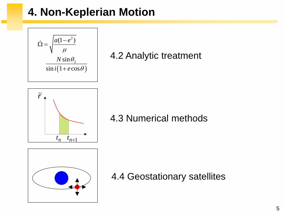
5
4 Non-Keplerian Motion
2
2
(1 )
sin
sin 1 cos
a e
N
i e
42 Analytic treatment
43 Numerical methods
nt 1nt
r
44 Geostationary satellites
6
4 Non-Keplerian Motion
42 Analytic treatment
421 Variation of parameters
422 Non-spherical Earth
423 J2 propagator in STK
424 Atmospheric drag
425 Third-body perturbations
426 SGP4 propagator in STK
427 Solar radiation pressure
2
2
(1 )
sin
sin 1 cos
a e
N
i e
7
Analytic Treatment Definition
Position and velocity at a requested time are computed
directly from initial conditions in a single step
Analytic propagators use a closed-form solution of the
time-dependent motion of a satellite
Mainly used for the two dominant perturbations drag and
earth oblateness
42 Analytic treatment
8
Analytic Treatment Pros and Cons
Useful for mission planning and analysis (fast and insight)
Though the numerical integration methods can generate more
accurate ephemeris of a satellite with respect to a complex force
model the analytical solutions represent a manifold of solutions for
a large domain of initial conditions and parameters
But less accurate than numerical integration
Be aware of the assumptions made
42 Analytic treatment
9
Assumption for Analytic Developments
The magnitude of the disturbing force is assumed to be
much smaller than the magnitude of the attraction of the
satellite for the primary
3 perturbedr
r r a
perturbed a r
42 Analytic treatment
10
Variation of Parameters (VOP)
Originally developed by Euler and improved by Lagrange
(conservative) and Gauss (nonconservative)
It is called variation of parameters because the orbital
elements (ie the constant parameters in the two-body
equations) are changing in the presence of perturbations
The VOP equations are a system of first-order ODEs that
describe the rates of change of the orbital elements
421 Variation of parameters
a i e M
11
Disturbing Acceleration (Specific Force)
ˆ ˆ ˆRperturbed R T NT N a F e e e
2
421 Variation of parameters
Rotating basis whose
origin is fixed to the
satellite
12
Perturbation Equations (Gauss)
421 Variation of parameters
2a
Chapter 2
2
2
2
2
aa
2
h
r
2 2
2
1 sin sin
1 cos
h r e er r
e h h
(1)
(2)
(3)
The generating solution is that of the 2-body problem
ˆ ˆR Tr r rR r T Fr F e e (4)
Time rate-of-change
of the work done by
the disturbing force
13
Perturbation Equations (Gauss)
421 Variation of parameters
(1)
(2)
(3)
(4)
2 2 2
2
2 sin 2sin
2 sin 1 cos
a e h a ha R T e R T
h r h r
aRe T e
h
2(1 )h a e
3
22 sin 1 cos
1
aa Re T e
e
Chapter 2
14
Perturbation Equations (Gauss)
3
22 Resin 1 cos
1
aa T e
e
2(1 )
sin cos cosa e
e R T E
2
2cos(1 )
1 cos
Na ei
e
JE Prussing BA Conway Orbital Mechanics Oxford University Press
421 Variation of parameters
2 sin 2 cos1 (1 )cos cos
1 cos
T ea ei R
e e
2 2(1 ) 2 cos cos sin 2 cos with
1 cos
e R e e T eaM nt
e e
2
2sin(1 )
sin 1 cos
Na e
i e
15
Perturbation Equations (Gauss)
Limited to eccentricities less than 1
Singular for e=0 sin i=0 (use of equinoctial elements)
In what follows we apply the Gauss equations to Earth
oblateness and drag Analytical expressions for third-body
and solar radiation forces are far less common because
their effects are much smaller for many orbits
421 Variation of parameters
16
Non-spherical Earth J2
Focus on the oblateness through the first zonal harmonic
J2 (tesseral and sectorial coefficients ignored)
The J2 effect can still be viewed a small perturbation when
compared to the attraction of the spherical Earth
422 Non-spherical Earth
17
Disturbing Acceleration (Specific Force)
2 2 222
4
3 1 3sin sinsin sin cos sin sin cos
2r T N
J R ii i i
r
F e e e
422 Non-spherical Earth
2 2
2
3sin 11
2
satRU J
r r
1 1 ˆˆ ˆ with cos
Ur r r
F r φ λ
Chapter 4A
18
Physical Interpretation of the Perturbation
The oblateness means that the force of gravity is no longer
within the orbital plane non-planar motion will result
The equatorial bulge exerts a force that pulls the satellite
back to the equatorial plane and thus tries to align the
orbital plane with the equator
Due to its angular momentum the orbit behaves like a
spinning top and reacts with a precessional motion of the
orbital plane (the orbital plane of the satellite to rotate in
inertial space)
422 Non-spherical Earth
19
Physical Interpretation of the Perturbation
422 Non-spherical Earth
20
Effect of Perturbations on Orbital Elements
Secular rate of change average rate of change over many
orbits
Periodic rate of change rate of change within one orbit
(J2 ~ 8-10km with a period equal to the orbital period)
422 Non-spherical Earth
21
Effect of Perturbations on Orbital Elements
Periodic
Secular
422 Non-spherical Earth
22
Secular Effects on Orbital Elements
Nodal regression regression of the nodal line
Apsidal rotation rotation of the apse line
Mean anomaly
No secular variations for a e i
422 Non-spherical Earth
2
2
2 2 7 20
1 3cos
2 (1 )
T
avg
J Rdt i
T e a
2
22
2 2 7 20
1 34 5sin
4 (1 )
T
avg
J Rdt i
T e a
23
Secular Effects Node Line
2
2
2 2 7 20
1 3cos
2 (1 )
T
avg
J Rdt i
T e a
For posigrade orbits the node line drifts westward
(regression of the nodes) And conversely
0 90 0i
For polar orbits the node line is stationary
90 0i
422 Non-spherical Earth
Vallado Fundamental of
Astrodynamics and
Applications Kluwer 2001
25
Exploitation Sun-Synchronous Orbits
The orbital plane makes a constant angle with the radial
from the sun
422 Non-spherical Earth
26
Exploitation Sun-Synchronous Orbits
The orbital plane must rotate in inertial space with the
angular velocity of the Earth in its orbit around the Sun
360ordm per 36526 days or 09856ordm per day
The satellite sees any given swath of the planet under
nearly the same condition of daylight or darkness day after
day
422 Non-spherical Earth
27
Existing Satellites
SPOT-5
(820 kms 987ordm)
NOAAPOES
(833 kms 987ordm)
28
Secular Effects Apse Line
2
22
2 2 7 20
1 34 5sin
4 (1 )
T
avg
J Rdt i
T e a
The perigee advances in the direction of the motion
of the satellite And conversely
0 634 or 1166 180 0i i
The apse line does not move
634 or 1166 0i i
422 Non-spherical Earth
Vallado Fundamental of
Astrodynamics and
Applications Kluwer 2001
30
Exploitation Molniya Orbits
A geostationary satellite cannot view effectively the far
northern latitudes into which Russian territory extends
(+ costly plane change maneuver for the launch vehicle )
Molniya telecommunications satellites are launched from
Plesetsk (628ordmN) into 63ordm inclination orbits having a
period of 12 hours
3
2 the apse line is 53000km longellip
aT
422 Non-spherical Earth
31
Analytic Propagators in STK 2-body J2
2-body constant orbital elements
J2 accounts for secular variations in the orbit elements
due to Earth oblateness periodic variations are
neglected
423 J2 propagator in STK
32
J2 Propagator Underlying Equations
423 J2 propagator in STK
33
2-body and J2 Propagators Applied to ISS
Two-body propagator J2 propagator
423 J2 propagator in STK
34
HPOP and J2 Propagators Applied to ISS
Nodal regression of the ISS
35
Effects of Atmospheric Drag Semi-Major Axis
2a
Lecture 2
2
2
2
2
aa
gt0
Because drag causes the dissipation of mechanical energy
from the system the semimajor axis contracts
424 Atmospheric drag
Drag paradox the effect of atmospheric drag is to increase
the satellite speed and kinetic energy
36
Effects of Atmospheric Drag Semi-Major Axis
21 10
2 2D r D
A AN R T C v C
m m a
0D
Aa a C
m
2
Df i f i
C Aa a t t
m
is assumed constant
424 Atmospheric drag
3
22 Resin 1 cos
1
aa T e
e
Circular orbit
37
Effects of Atmospheric Drag Orbit Plane
2
2sin(1 )
sin 1 cos
Na e
i e
2
2cos(1 )
1 cos
Na ei
e
The orientation of the orbit plane is not changed by drag
424 Atmospheric drag
38
Effects of Atmospheric Drag Apogee Perigee
Apogee height changes drastically perigee height remains
relatively constant
424 Atmospheric drag
Vallado Fundamental of Astrodynamics and Applications Kluwer 2001
39
Effects of Atmospheric Drag Eccentricity
Vallado Fundamental of Astrodynamics and Applications Kluwer 2001
424 Atmospheric drag
40
Early Reentry of Skylab (1979)
Increased solar activity which
increased drag on Skylab led to
an early reentry
Earth reentry footprint could not
be accurately predicted (due to
tumbling and other parameters)
Debris was found around
Esperance (31ndash34degS 122ndash
126degE) The Shire of Esperance
fined the United States $400 for
littering a fine which to this day
remains unpaid
424 Atmospheric drag
41
Lost of ASCA Satellite (2000)
July 15 2000 a strong solar
flare heated the Earthrsquos
atmosphere increasing the
air density to a value 100
times greater than that for
which its ADCS had been
designed to cope The
magnetorquers were unable
to compensate and the
satellite was lost
httpheasarcgsfcnasagovdocsascasafemodehtml
424 Atmospheric drag
42
Effects of Third-Body Perturbations
The only secular perturbations are in the node and in the
perigee
For near-Earth orbits the dominance of the oblateness
dictates that the orbital plane regresses about the polar
axis For higher orbits the regression will be about some
mean pole lying between the Earthrsquos pole and the ecliptic
pole
Many geosynchronous satellites launched 30 years ago
now have inclinations of up to plusmn15ordm collision avoidance
as the satellites drift back through the GEO belt
425 Third-body perturbations
43
Effects of Third-Body Perturbations
Vallado Fundamental of Astrodynamics and Applications Kluwer 2001
The Sunrsquos attraction
tends to turn the
satellite ring into the
ecliptic The orbit
precesses about the
pole of the ecliptic
425 Third-body perturbations
44
STK Analytic Propagator (SGP4)
The J2 propagator does not include drag
SGP4 which stands for Simplified General Perturbations
Satellite Orbit Model 4 is a NASANORAD algorithm
426 SGP4 propagator in STK
45
STK Analytic Propagator (SGP4)
Several assumptions propagation valid for short durations
(3-10 days)
TLE data should be used as the input (see Lecture 03)
It considers secular and periodic variations due to Earth
oblateness solar and lunar gravitational effects and
orbital decay using a drag model
426 SGP4 propagator in STK
46
SGP4 Applied to ISS RAAN
426 SGP4 propagator in STK
47
SGP4 Applied to ISS Semi-Major Axis
426 SGP4 propagator in STK
48
Further Reading on the Web Site
426 SGP4 propagator in STK
49
Effects of Solar Radiation Pressure
The effects are usually small for most satellites
Satellites with very low mass and large surface area are
more affected
427 Solar radiation pressure
Vallado Fundamental of
Astrodynamics and
Applications Kluwer
2001
51
Secular Effects Orders of Magnitude
Vallado Fundamental of Astrodynamics and Applications Kluwer 2001
52
Periodic Effects Orders of Magnitude
Vallado Fundamental of Astrodynamics and Applications Kluwer 2001
53
4 Non-Keplerian Motion
2
2
(1 )
sin
sin 1 cos
a e
N
i e
43 Numerical methods
431 Orbit prediction
432 Numerical integration
433 Single-step methods Runge-Kutta
434 Multi-step methods
435 Integrator and step size selection
436 ISS example
nt 1nt
r
54
2-body analytic propagator (constant orbital elements)
J2 analytic propagator (secular variations in the orbit
elements due to Earth oblateness
HPOP numerical integration of the equations of motion
(periodic and secular effects included)
STK Propagators
431 Orbit prediction
Accurate
Versatile
Errors accumulation
for long intervals
Computationally
intensive
55
Real-Life Example German Aerospace Agency
431 Orbit prediction
56
Real-Life Example German Aerospace Agency
57
Further Reading on the Web Site
431 Orbit prediction
58
Real-Life Example Envisat
httpnngesocesadeenvisat
ENVpredhtml
431 Orbit prediction
Why do the
predictions degrade
for lower altitudes
60
NASA began the first complex numerical integrations
during the late 1960s and early 1970s
Did you Know
1969 1968
431 Orbit prediction
61
What is Numerical Integration
1n nt t t
3 perturbedr
r r a
Given
Compute
( ) ( )n nt tr r
1 1( ) ( )n nt t r r
432 Numerical integration
62
State-Space Formulation
3 perturbedr
r r a
( )f tu u
ru
r
6-dimensional
state vector
432 Numerical integration
63
How to Perform Numerical Integration
2( )( ) ( ) ( ) ( ) ( )
2
ss
n n n n n s
h hf t h f t hf t f t f t R
s
Taylor series expansion
( )ntu
1( )nt u
432 Numerical integration
64
First-Order Taylor Approximation (Euler)
1
( ) ( ) ( )
( )
n n n
n n n n
t t t t t
t f t
u u u
u u uEuler step
0 1 2 3 4 5 60
5
10
15
20
25
30
35
40
Time t (s)
x(t
)=t2
Exact solution
The stepsize has to be extremely
small for accurate predictions
and it is necessary to develop
more effective algorithms
along the tangent
432 Numerical integration
65
Numerical Integration Methods
1 1 1
1 0
m m
n j n j j n j
j j
t
u u u
0 0
Implicit the solution method becomes
iterative in the nonlinear case
0 0 Explicit un+1 can be deduced directly from
the results at the previous time steps
=0
for 1
j j
j
Single-step the system at time tn+1
only depends on the previous state tn
State vector
0
for 1
j j
j
Multi-step the system at time tn+1 depends
several previous states tntn-1etc
432 Numerical integration
66
Examples Implicit vs Explicit
Trapezoidal rule (implicit)
nt 1nt
Euler forward (explicit)
nt 1nt
Euler backward (implicit)
nt 1nt
1n n nt u u u
1 1n n nt u u u
1
12
n n
n n t
u uu u
r
r
r
432 Numerical integration
67
A variety of methods has been applied in astrodynamics
Each of these methods has its own advantages and
drawbacks
Accuracy what is the order of the integration scheme
Efficiency how many function calls
Versatility can it be applied to a wide range of problems
Complexity is it easy to implement and use
Step size automatic step size control
Why Different Methods
431 Orbit prediction
68
Runge-Kutta Family Single-Step
Perhaps the most well-known numerical integrator
Difference with traditional Taylor series integrators the RK
family only requires the first derivative but several
evaluations are needed to move forward one step in time
Different variants explicit embedded etc
433 Single-step methods Runge-Kutta
69
Runge-Kutta Family Single-Step
with ( ) ( )t f tu u 0 0( )t u u
1
1
s
n n i i
i
t b
u u k
1 1
1
1
2
n n
i
i n ij j n i
j
f t c t
f t a t c t i s
k u
k u k
Slopes at
various points
within the
integration step
433 Single-step methods Runge-Kutta
70
Runge-Kutta Family Single-Step
Butcher Tableau
The Runge-Kutta methods are fully described by the
coefficients
c1
c2
cs
a21
as1
b1
as2
b2
ass-1
bs-1 hellip
hellip
hellip hellip hellip
bs
1
1
1
1
1
0
s
i
i
i
i ij
j
b
c
c a
433 Single-step methods Runge-Kutta
71
RK4 (Explicit)
1 2 3 41
2 2
6n n t
k k k ku u
Butcher Tableau
1
2 1
3 2
4 3
2 2
2 2
n n
n n
n n
n n
f t
t tf t
t tf t
f t t t
k u
k u k
k u k
k u k
433 Single-step methods Runge-Kutta
72
RK4 (Explicit)
1 2 3 41
2 2
6n n t
k k k ku u
1
2 1
3 2
4 3
2 2
2 2
n n
n n
n n
n n
f t
t tf t
t tf t
f t t t
k u
k u k
k u k
k u k
Slope at the beginning
Slope at the midpoint (k1 is
used to determine the value
of u Euler)
Slope at the midpoint (k2 is
now used)
Slope at the end
Estimated slope
(weighted average)
433 Single-step methods Runge-Kutta
73
RK4 (Explicit)
nt 2nt t nt t
1k3k
2k
4k
Estimate at new
time
u
433 Single-step methods Runge-Kutta
74
RK4 (Explicit)
The local truncation error for a 4th order RK is O(h5)
The accuracy is comparable to that of a 4th order Taylor
series but the Runge-Kutta method avoids the
calculation of higher-order derivatives
Easy to use and implement
The step size is fixed
433 Single-step methods Runge-Kutta
75
RK4 in STK
433 Single-step methods Runge-Kutta
76
Embedded Methods
They produce an estimate of the local truncation error
adjust the step size to keep local truncation errors
within some tolerances
This is done by having two methods in the tableau one with
order p and one with order p+1 with the same set of
function evaluations
( 1) ( 1) ( 1)
1
1
sp p p
n n i i
i
t b
u u k
( ) ( ) ( )
1
1
sp p p
n n i i
i
t b
u u k
433 Single-step methods Runge-Kutta
77
Embedded Methods
The two different approximations for the solution at each
step are compared
If the two answers are in close agreement the approximation is
accepted
If the two answers do not agree to a specified accuracy the step
size is reduced
If the answers agree to more significant digits than required the
step size is increased
433 Single-step methods Runge-Kutta
78
Ode45 in Matlab Simulink
Runge-Kutta (45) pair of Dormand and Prince
Variable step size
Matlab help This should be the first solver you try
433 Single-step methods Runge-Kutta
79
Ode45 in Matlab Simulink
edit ode45
433 Single-step methods Runge-Kutta
80
Ode45 in Matlab Simulink
Be very careful with the default parameters
options = odeset(RelTol1e-8AbsTol1e-8)
433 Single-step methods Runge-Kutta
81
RKF 7(8) Default Method in STK
Runge-Kutta-Fehlberg integration method of 7th order
with 8th order error control for the integration step size
433 Single-step methods Runge-Kutta
83
Multi-Step Methods (Predictor-Corrector)
They estimate the state over time using previously
determined back values of the solution
Unlike RK methods they only perform one evaluation for
each step forward but they usually have a predictor and a
corrector formula
Adams() ndash Bashforth - Moulton Gauss - Jackson
() The first with Le Verrier to predict the existence and position of Neptune
434 Multi-step methods
84
Multi-Step Methods Principle
( ) ( )t f tu u1
1( ) ( ) ( ) n
n
t
n nt
t t f t dt
u u u
unknown
Replace it by a
polynomial that
interpolates the
previous values Four function values
interpolated by a
third-order polynomial
t
u
434 Multi-step methods
85
Multi-Step Methods Initiation
with ( ) ( )t f tu u 0 0( )t u u
What is the inherent problem
t
u
434 Multi-step methods
86
Multi-Step Methods Initiation
Because these methods require back values they are not
self-starting
One may for instance use of a single-step method to
compute the first four values
434 Multi-step methods
87
Gauss-Jackson in STK
One of the most recommendable fixed-stepsize multistep
methods for orbit computations
88
Integrator Selection
435 Integrator and step size selection
Montenbruck and Gill
Satellite orbits Springer
2000
89
Integrator Selection
Pros
Very fast
Cons
Special starting procedure
Fixed time steps
Error control
Pros
Plug and play
Error control
Cons
Slower
Multi-step Single step
435 Integrator and step size selection
90
Why is the Step Size So Critical
Theoretical arguments
1 The accuracy and the stability of the algorithm are
directly related to the step size
2 Nonlinear equations of motion
Data for Landsat 4 and 6 in circular orbits around 800km
indicates that a one-minute step size yields about 47m
error
A three-minute step size produces about a 900m error
435 Integrator and step size selection
91
Why is the Step Size So Critical
More practical arguments
1 The computation time is directly related to the
step size
2 The particular choice of step size depends on the
most rapidly varying component in the disturbing
functions (eg 50 x 50 gravity field)
435 Integrator and step size selection
92
Appropriate Step Size
The problem of determining an appropriate step size is a
challenge in any numerical process
Fixed step size (rule of thumb for standard
applications)
But an algorithm with variable step size is really
helpful The step size is chosen in such a way that
each step contributes uniformly to the total integration
error
100
orbitTt
435 Integrator and step size selection
93
Three Examples XMM OUFTI-1 ISS
Can you plot the step size vs true anomaly
435 Integrator and step size selection
94
XMM Report in STK
435 Integrator and step size selection
95
XMM (e~08)
0 50 100 150 200 250 300 350 4000
1000
2000
3000
4000
5000
6000
True anomaly (deg)
Ste
p s
ize
(s)
435 Integrator and step size selection
96
ISS(e~0)
435 Integrator and step size selection
0 50 100 150 200 250 300 350 40030
35
40
45
50
55
60
65
70
True anomaly (deg)
Ste
p s
ize
(s)
97
ldquoDifficultrdquo Orbits
Automatic time step is especially nice on highly eccentric
orbits (Molniya XMM) These orbits are best computed
using variable step sizes to maintain some given level of
accuracy
Without this variable step size we waste a lot of time near
apoapsis when the integration is taking too small a step
Likewise the integrator may not be using a small enough step
size at periapsis where the satellite is traveling fast
435 Integrator and step size selection
98
HPOP Propagator ISS Example
1 Earthrsquos oblateness only
2 Drag only
3 Sun and moon only
4 SRP only
5 All together
436 ISS example
99
Earthrsquos Oblateness Only Ω
HPOP
J2
2-body
436 ISS example
100
Earthrsquos Oblateness Only i Ω a
HPOP with central body (20 + WGS84_EGM96)
(without dragSRPSun and Moon)
436 ISS example
101
Drag Only i Ω a
HPOP with drag ndash Harris Priester
(without oblatenessSRPSun and Moon)
436 ISS example
102
Drag Relationship with Eclipses
103
SRP Only i Ω a
HPOP with SRP
(without oblatenessdragSun and Moon)
436 ISS example
104
SRP Relationship with Eclipses
105
All Perturbations Together
436 ISS example
106
4 Non-Keplerian Motion
2
2
(1 )
sin
sin 1 cos
a e
N
i e
44 Geostationary satellites
107
Practical Example GEO Satellites
Nice illustration of
1 Perturbations of the 2-body problem
2 Secular and periodic contributions
3 Accuracy required by practical applications
4 The need for orbit correction and thrust forces
And it is a real-life example (telecommunications
meteorology)
44 GEO satellites
108
Three Main Perturbations for GEO Satellites
44 GEO satellites
1 Non-spherical Earth
2 SRP
3 Sun and Moon
109
Station Keeping of GEO Satellites
The effect of the perturbations is to cause the spacecraft
to drift away from its nominal station If the drift was
allowed to build up unchecked the spacecraft could
become useless
A station-keeping box is defined by a longitude and a
maximum authorized distance for satellite excursions in
longitude and latitude
For instance TC2 -8ordm plusmn 007ordm EW plusmn 005ordm NS
44 GEO satellites
110
East-West and North-South Drift
44 GEO satellites
NS drift
EW drift
What are the perturbations generating these drifts
111
East-West Drift
44 GEO satellites
A GEO satellite drifts in longitude due to the influence of
two main perturbations
1 The elliptic nature of the Earthrsquos equatorial cross-
section J22 (and not from the NS oblateness J2)
2
ΔV
ΔV vsat
vsat SRP
112
East-West Drift due to Equatorial Ellipticity
44 GEO satellites
113
East-West Drift due to Equatorial Ellipticity
44 GEO satellites
114
East-West Drift HPOP (20) vs HPOP (22)
44 GEO satellites
115
East-West Drift Stable Equilibirum
HPOP with 22
(without Sun and moonSRPdrag)
116
East-West Drift Stable Equilibirum
HPOP with 22
(without Sun and moonSRPdrag)
117
East-West Drift Stable Equilibirum
HPOP with 22
(without Sun and moonSRPdrag)
118
North-South Drift
The perturbations caused by the Sun and the Moon are
predominantly out-of-plane effects causing a change in
the inclination and in the right ascension of the orbit
ascending node
Similar effects on the orbit to those of the Earthrsquos
oblateness (but here with respect to the ecliptic)
A GEO satellite therefore drifts in latitude with a
fundamental period equal to the orbit period
119
North-South Drift
Period
HPOP with Sun and Moon
(without oblatenessSRPdrag)
120
North-South Drift
Period
HPOP with Sun and Moon
(without oblatenessSRPdrag)
121
Thrust Forces for Stationkeeping
GEO spacecraft require continual stationkeeping to stay
within the authorized box using onboard thrusters
44 GEO satellites
122
42 ANALYTIC TREATMENT
421 Variation of parameters
422 Non-spherical Earth
423 J2 propagator in STK
424 Atmospheric drag
425 Third-body perturbations
426 SGP4 propagator in STK
427 Solar radiation pressure
4 Non-Keplerian Motion
43 NUMERICAL METHODS
431 Orbit prediction
432 Numerical integration
433 Single-step methods Runge-Kutta
434 Multi-step methods
435 Integrator and step size selection
436 ISS example
44 GEOSTATIONARY SATELLITES
Gaeumltan Kerschen
Space Structures amp
Systems Lab (S3L)
4B Non-Keplerian Motion
Astrodynamics (AERO0024)
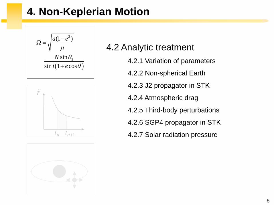
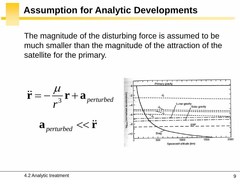
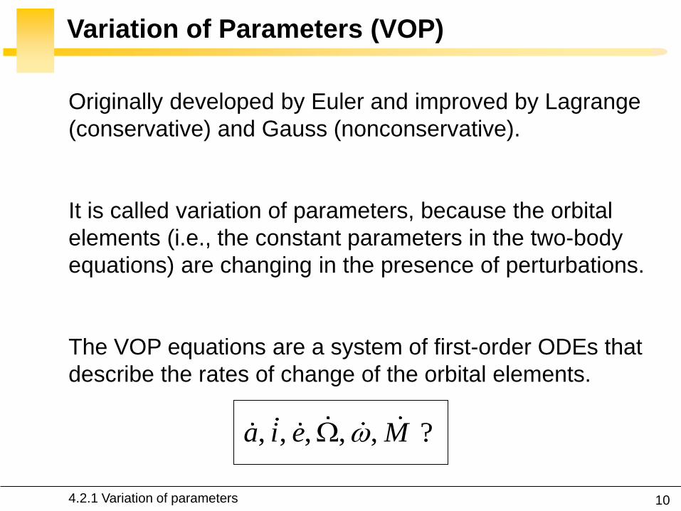
10
Variation of Parameters (VOP)
Originally developed by Euler and improved by Lagrange
(conservative) and Gauss (nonconservative)
It is called variation of parameters because the orbital
elements (ie the constant parameters in the two-body
equations) are changing in the presence of perturbations
The VOP equations are a system of first-order ODEs that
describe the rates of change of the orbital elements
421 Variation of parameters
a i e M
11
Disturbing Acceleration (Specific Force)
ˆ ˆ ˆRperturbed R T NT N a F e e e
2
421 Variation of parameters
Rotating basis whose
origin is fixed to the
satellite
12
Perturbation Equations (Gauss)
421 Variation of parameters
2a
Chapter 2
2
2
2
2
aa
2
h
r
2 2
2
1 sin sin
1 cos
h r e er r
e h h
(1)
(2)
(3)
The generating solution is that of the 2-body problem
ˆ ˆR Tr r rR r T Fr F e e (4)
Time rate-of-change
of the work done by
the disturbing force
13
Perturbation Equations (Gauss)
421 Variation of parameters
(1)
(2)
(3)
(4)
2 2 2
2
2 sin 2sin
2 sin 1 cos
a e h a ha R T e R T
h r h r
aRe T e
h
2(1 )h a e
3
22 sin 1 cos
1
aa Re T e
e
Chapter 2
14
Perturbation Equations (Gauss)
3
22 Resin 1 cos
1
aa T e
e
2(1 )
sin cos cosa e
e R T E
2
2cos(1 )
1 cos
Na ei
e
JE Prussing BA Conway Orbital Mechanics Oxford University Press
421 Variation of parameters
2 sin 2 cos1 (1 )cos cos
1 cos
T ea ei R
e e
2 2(1 ) 2 cos cos sin 2 cos with
1 cos
e R e e T eaM nt
e e
2
2sin(1 )
sin 1 cos
Na e
i e
15
Perturbation Equations (Gauss)
Limited to eccentricities less than 1
Singular for e=0 sin i=0 (use of equinoctial elements)
In what follows we apply the Gauss equations to Earth
oblateness and drag Analytical expressions for third-body
and solar radiation forces are far less common because
their effects are much smaller for many orbits
421 Variation of parameters
16
Non-spherical Earth J2
Focus on the oblateness through the first zonal harmonic
J2 (tesseral and sectorial coefficients ignored)
The J2 effect can still be viewed a small perturbation when
compared to the attraction of the spherical Earth
422 Non-spherical Earth
17
Disturbing Acceleration (Specific Force)
2 2 222
4
3 1 3sin sinsin sin cos sin sin cos
2r T N
J R ii i i
r
F e e e
422 Non-spherical Earth
2 2
2
3sin 11
2
satRU J
r r
1 1 ˆˆ ˆ with cos
Ur r r
F r φ λ
Chapter 4A
18
Physical Interpretation of the Perturbation
The oblateness means that the force of gravity is no longer
within the orbital plane non-planar motion will result
The equatorial bulge exerts a force that pulls the satellite
back to the equatorial plane and thus tries to align the
orbital plane with the equator
Due to its angular momentum the orbit behaves like a
spinning top and reacts with a precessional motion of the
orbital plane (the orbital plane of the satellite to rotate in
inertial space)
422 Non-spherical Earth
19
Physical Interpretation of the Perturbation
422 Non-spherical Earth
20
Effect of Perturbations on Orbital Elements
Secular rate of change average rate of change over many
orbits
Periodic rate of change rate of change within one orbit
(J2 ~ 8-10km with a period equal to the orbital period)
422 Non-spherical Earth
21
Effect of Perturbations on Orbital Elements
Periodic
Secular
422 Non-spherical Earth
22
Secular Effects on Orbital Elements
Nodal regression regression of the nodal line
Apsidal rotation rotation of the apse line
Mean anomaly
No secular variations for a e i
422 Non-spherical Earth
2
2
2 2 7 20
1 3cos
2 (1 )
T
avg
J Rdt i
T e a
2
22
2 2 7 20
1 34 5sin
4 (1 )
T
avg
J Rdt i
T e a
23
Secular Effects Node Line
2
2
2 2 7 20
1 3cos
2 (1 )
T
avg
J Rdt i
T e a
For posigrade orbits the node line drifts westward
(regression of the nodes) And conversely
0 90 0i
For polar orbits the node line is stationary
90 0i
422 Non-spherical Earth
Vallado Fundamental of
Astrodynamics and
Applications Kluwer 2001
25
Exploitation Sun-Synchronous Orbits
The orbital plane makes a constant angle with the radial
from the sun
422 Non-spherical Earth
26
Exploitation Sun-Synchronous Orbits
The orbital plane must rotate in inertial space with the
angular velocity of the Earth in its orbit around the Sun
360ordm per 36526 days or 09856ordm per day
The satellite sees any given swath of the planet under
nearly the same condition of daylight or darkness day after
day
422 Non-spherical Earth
27
Existing Satellites
SPOT-5
(820 kms 987ordm)
NOAAPOES
(833 kms 987ordm)
28
Secular Effects Apse Line
2
22
2 2 7 20
1 34 5sin
4 (1 )
T
avg
J Rdt i
T e a
The perigee advances in the direction of the motion
of the satellite And conversely
0 634 or 1166 180 0i i
The apse line does not move
634 or 1166 0i i
422 Non-spherical Earth
Vallado Fundamental of
Astrodynamics and
Applications Kluwer 2001
30
Exploitation Molniya Orbits
A geostationary satellite cannot view effectively the far
northern latitudes into which Russian territory extends
(+ costly plane change maneuver for the launch vehicle )
Molniya telecommunications satellites are launched from
Plesetsk (628ordmN) into 63ordm inclination orbits having a
period of 12 hours
3
2 the apse line is 53000km longellip
aT
422 Non-spherical Earth
31
Analytic Propagators in STK 2-body J2
2-body constant orbital elements
J2 accounts for secular variations in the orbit elements
due to Earth oblateness periodic variations are
neglected
423 J2 propagator in STK
32
J2 Propagator Underlying Equations
423 J2 propagator in STK
33
2-body and J2 Propagators Applied to ISS
Two-body propagator J2 propagator
423 J2 propagator in STK
34
HPOP and J2 Propagators Applied to ISS
Nodal regression of the ISS
35
Effects of Atmospheric Drag Semi-Major Axis
2a
Lecture 2
2
2
2
2
aa
gt0
Because drag causes the dissipation of mechanical energy
from the system the semimajor axis contracts
424 Atmospheric drag
Drag paradox the effect of atmospheric drag is to increase
the satellite speed and kinetic energy
36
Effects of Atmospheric Drag Semi-Major Axis
21 10
2 2D r D
A AN R T C v C
m m a
0D
Aa a C
m
2
Df i f i
C Aa a t t
m
is assumed constant
424 Atmospheric drag
3
22 Resin 1 cos
1
aa T e
e
Circular orbit
37
Effects of Atmospheric Drag Orbit Plane
2
2sin(1 )
sin 1 cos
Na e
i e
2
2cos(1 )
1 cos
Na ei
e
The orientation of the orbit plane is not changed by drag
424 Atmospheric drag
38
Effects of Atmospheric Drag Apogee Perigee
Apogee height changes drastically perigee height remains
relatively constant
424 Atmospheric drag
Vallado Fundamental of Astrodynamics and Applications Kluwer 2001
39
Effects of Atmospheric Drag Eccentricity
Vallado Fundamental of Astrodynamics and Applications Kluwer 2001
424 Atmospheric drag
40
Early Reentry of Skylab (1979)
Increased solar activity which
increased drag on Skylab led to
an early reentry
Earth reentry footprint could not
be accurately predicted (due to
tumbling and other parameters)
Debris was found around
Esperance (31ndash34degS 122ndash
126degE) The Shire of Esperance
fined the United States $400 for
littering a fine which to this day
remains unpaid
424 Atmospheric drag
41
Lost of ASCA Satellite (2000)
July 15 2000 a strong solar
flare heated the Earthrsquos
atmosphere increasing the
air density to a value 100
times greater than that for
which its ADCS had been
designed to cope The
magnetorquers were unable
to compensate and the
satellite was lost
httpheasarcgsfcnasagovdocsascasafemodehtml
424 Atmospheric drag
42
Effects of Third-Body Perturbations
The only secular perturbations are in the node and in the
perigee
For near-Earth orbits the dominance of the oblateness
dictates that the orbital plane regresses about the polar
axis For higher orbits the regression will be about some
mean pole lying between the Earthrsquos pole and the ecliptic
pole
Many geosynchronous satellites launched 30 years ago
now have inclinations of up to plusmn15ordm collision avoidance
as the satellites drift back through the GEO belt
425 Third-body perturbations
43
Effects of Third-Body Perturbations
Vallado Fundamental of Astrodynamics and Applications Kluwer 2001
The Sunrsquos attraction
tends to turn the
satellite ring into the
ecliptic The orbit
precesses about the
pole of the ecliptic
425 Third-body perturbations
44
STK Analytic Propagator (SGP4)
The J2 propagator does not include drag
SGP4 which stands for Simplified General Perturbations
Satellite Orbit Model 4 is a NASANORAD algorithm
426 SGP4 propagator in STK
45
STK Analytic Propagator (SGP4)
Several assumptions propagation valid for short durations
(3-10 days)
TLE data should be used as the input (see Lecture 03)
It considers secular and periodic variations due to Earth
oblateness solar and lunar gravitational effects and
orbital decay using a drag model
426 SGP4 propagator in STK
46
SGP4 Applied to ISS RAAN
426 SGP4 propagator in STK
47
SGP4 Applied to ISS Semi-Major Axis
426 SGP4 propagator in STK
48
Further Reading on the Web Site
426 SGP4 propagator in STK
49
Effects of Solar Radiation Pressure
The effects are usually small for most satellites
Satellites with very low mass and large surface area are
more affected
427 Solar radiation pressure
Vallado Fundamental of
Astrodynamics and
Applications Kluwer
2001
51
Secular Effects Orders of Magnitude
Vallado Fundamental of Astrodynamics and Applications Kluwer 2001
52
Periodic Effects Orders of Magnitude
Vallado Fundamental of Astrodynamics and Applications Kluwer 2001
53
4 Non-Keplerian Motion
2
2
(1 )
sin
sin 1 cos
a e
N
i e
43 Numerical methods
431 Orbit prediction
432 Numerical integration
433 Single-step methods Runge-Kutta
434 Multi-step methods
435 Integrator and step size selection
436 ISS example
nt 1nt
r
54
2-body analytic propagator (constant orbital elements)
J2 analytic propagator (secular variations in the orbit
elements due to Earth oblateness
HPOP numerical integration of the equations of motion
(periodic and secular effects included)
STK Propagators
431 Orbit prediction
Accurate
Versatile
Errors accumulation
for long intervals
Computationally
intensive
55
Real-Life Example German Aerospace Agency
431 Orbit prediction
56
Real-Life Example German Aerospace Agency
57
Further Reading on the Web Site
431 Orbit prediction
58
Real-Life Example Envisat
httpnngesocesadeenvisat
ENVpredhtml
431 Orbit prediction
Why do the
predictions degrade
for lower altitudes
60
NASA began the first complex numerical integrations
during the late 1960s and early 1970s
Did you Know
1969 1968
431 Orbit prediction
61
What is Numerical Integration
1n nt t t
3 perturbedr
r r a
Given
Compute
( ) ( )n nt tr r
1 1( ) ( )n nt t r r
432 Numerical integration
62
State-Space Formulation
3 perturbedr
r r a
( )f tu u
ru
r
6-dimensional
state vector
432 Numerical integration
63
How to Perform Numerical Integration
2( )( ) ( ) ( ) ( ) ( )
2
ss
n n n n n s
h hf t h f t hf t f t f t R
s
Taylor series expansion
( )ntu
1( )nt u
432 Numerical integration
64
First-Order Taylor Approximation (Euler)
1
( ) ( ) ( )
( )
n n n
n n n n
t t t t t
t f t
u u u
u u uEuler step
0 1 2 3 4 5 60
5
10
15
20
25
30
35
40
Time t (s)
x(t
)=t2
Exact solution
The stepsize has to be extremely
small for accurate predictions
and it is necessary to develop
more effective algorithms
along the tangent
432 Numerical integration
65
Numerical Integration Methods
1 1 1
1 0
m m
n j n j j n j
j j
t
u u u
0 0
Implicit the solution method becomes
iterative in the nonlinear case
0 0 Explicit un+1 can be deduced directly from
the results at the previous time steps
=0
for 1
j j
j
Single-step the system at time tn+1
only depends on the previous state tn
State vector
0
for 1
j j
j
Multi-step the system at time tn+1 depends
several previous states tntn-1etc
432 Numerical integration
66
Examples Implicit vs Explicit
Trapezoidal rule (implicit)
nt 1nt
Euler forward (explicit)
nt 1nt
Euler backward (implicit)
nt 1nt
1n n nt u u u
1 1n n nt u u u
1
12
n n
n n t
u uu u
r
r
r
432 Numerical integration
67
A variety of methods has been applied in astrodynamics
Each of these methods has its own advantages and
drawbacks
Accuracy what is the order of the integration scheme
Efficiency how many function calls
Versatility can it be applied to a wide range of problems
Complexity is it easy to implement and use
Step size automatic step size control
Why Different Methods
431 Orbit prediction
68
Runge-Kutta Family Single-Step
Perhaps the most well-known numerical integrator
Difference with traditional Taylor series integrators the RK
family only requires the first derivative but several
evaluations are needed to move forward one step in time
Different variants explicit embedded etc
433 Single-step methods Runge-Kutta
69
Runge-Kutta Family Single-Step
with ( ) ( )t f tu u 0 0( )t u u
1
1
s
n n i i
i
t b
u u k
1 1
1
1
2
n n
i
i n ij j n i
j
f t c t
f t a t c t i s
k u
k u k
Slopes at
various points
within the
integration step
433 Single-step methods Runge-Kutta
70
Runge-Kutta Family Single-Step
Butcher Tableau
The Runge-Kutta methods are fully described by the
coefficients
c1
c2
cs
a21
as1
b1
as2
b2
ass-1
bs-1 hellip
hellip
hellip hellip hellip
bs
1
1
1
1
1
0
s
i
i
i
i ij
j
b
c
c a
433 Single-step methods Runge-Kutta
71
RK4 (Explicit)
1 2 3 41
2 2
6n n t
k k k ku u
Butcher Tableau
1
2 1
3 2
4 3
2 2
2 2
n n
n n
n n
n n
f t
t tf t
t tf t
f t t t
k u
k u k
k u k
k u k
433 Single-step methods Runge-Kutta
72
RK4 (Explicit)
1 2 3 41
2 2
6n n t
k k k ku u
1
2 1
3 2
4 3
2 2
2 2
n n
n n
n n
n n
f t
t tf t
t tf t
f t t t
k u
k u k
k u k
k u k
Slope at the beginning
Slope at the midpoint (k1 is
used to determine the value
of u Euler)
Slope at the midpoint (k2 is
now used)
Slope at the end
Estimated slope
(weighted average)
433 Single-step methods Runge-Kutta
73
RK4 (Explicit)
nt 2nt t nt t
1k3k
2k
4k
Estimate at new
time
u
433 Single-step methods Runge-Kutta
74
RK4 (Explicit)
The local truncation error for a 4th order RK is O(h5)
The accuracy is comparable to that of a 4th order Taylor
series but the Runge-Kutta method avoids the
calculation of higher-order derivatives
Easy to use and implement
The step size is fixed
433 Single-step methods Runge-Kutta
75
RK4 in STK
433 Single-step methods Runge-Kutta
76
Embedded Methods
They produce an estimate of the local truncation error
adjust the step size to keep local truncation errors
within some tolerances
This is done by having two methods in the tableau one with
order p and one with order p+1 with the same set of
function evaluations
( 1) ( 1) ( 1)
1
1
sp p p
n n i i
i
t b
u u k
( ) ( ) ( )
1
1
sp p p
n n i i
i
t b
u u k
433 Single-step methods Runge-Kutta
77
Embedded Methods
The two different approximations for the solution at each
step are compared
If the two answers are in close agreement the approximation is
accepted
If the two answers do not agree to a specified accuracy the step
size is reduced
If the answers agree to more significant digits than required the
step size is increased
433 Single-step methods Runge-Kutta
78
Ode45 in Matlab Simulink
Runge-Kutta (45) pair of Dormand and Prince
Variable step size
Matlab help This should be the first solver you try
433 Single-step methods Runge-Kutta
79
Ode45 in Matlab Simulink
edit ode45
433 Single-step methods Runge-Kutta
80
Ode45 in Matlab Simulink
Be very careful with the default parameters
options = odeset(RelTol1e-8AbsTol1e-8)
433 Single-step methods Runge-Kutta
81
RKF 7(8) Default Method in STK
Runge-Kutta-Fehlberg integration method of 7th order
with 8th order error control for the integration step size
433 Single-step methods Runge-Kutta
83
Multi-Step Methods (Predictor-Corrector)
They estimate the state over time using previously
determined back values of the solution
Unlike RK methods they only perform one evaluation for
each step forward but they usually have a predictor and a
corrector formula
Adams() ndash Bashforth - Moulton Gauss - Jackson
() The first with Le Verrier to predict the existence and position of Neptune
434 Multi-step methods
84
Multi-Step Methods Principle
( ) ( )t f tu u1
1( ) ( ) ( ) n
n
t
n nt
t t f t dt
u u u
unknown
Replace it by a
polynomial that
interpolates the
previous values Four function values
interpolated by a
third-order polynomial
t
u
434 Multi-step methods
85
Multi-Step Methods Initiation
with ( ) ( )t f tu u 0 0( )t u u
What is the inherent problem
t
u
434 Multi-step methods
86
Multi-Step Methods Initiation
Because these methods require back values they are not
self-starting
One may for instance use of a single-step method to
compute the first four values
434 Multi-step methods
87
Gauss-Jackson in STK
One of the most recommendable fixed-stepsize multistep
methods for orbit computations
88
Integrator Selection
435 Integrator and step size selection
Montenbruck and Gill
Satellite orbits Springer
2000
89
Integrator Selection
Pros
Very fast
Cons
Special starting procedure
Fixed time steps
Error control
Pros
Plug and play
Error control
Cons
Slower
Multi-step Single step
435 Integrator and step size selection
90
Why is the Step Size So Critical
Theoretical arguments
1 The accuracy and the stability of the algorithm are
directly related to the step size
2 Nonlinear equations of motion
Data for Landsat 4 and 6 in circular orbits around 800km
indicates that a one-minute step size yields about 47m
error
A three-minute step size produces about a 900m error
435 Integrator and step size selection
91
Why is the Step Size So Critical
More practical arguments
1 The computation time is directly related to the
step size
2 The particular choice of step size depends on the
most rapidly varying component in the disturbing
functions (eg 50 x 50 gravity field)
435 Integrator and step size selection
92
Appropriate Step Size
The problem of determining an appropriate step size is a
challenge in any numerical process
Fixed step size (rule of thumb for standard
applications)
But an algorithm with variable step size is really
helpful The step size is chosen in such a way that
each step contributes uniformly to the total integration
error
100
orbitTt
435 Integrator and step size selection
93
Three Examples XMM OUFTI-1 ISS
Can you plot the step size vs true anomaly
435 Integrator and step size selection
94
XMM Report in STK
435 Integrator and step size selection
95
XMM (e~08)
0 50 100 150 200 250 300 350 4000
1000
2000
3000
4000
5000
6000
True anomaly (deg)
Ste
p s
ize
(s)
435 Integrator and step size selection
96
ISS(e~0)
435 Integrator and step size selection
0 50 100 150 200 250 300 350 40030
35
40
45
50
55
60
65
70
True anomaly (deg)
Ste
p s
ize
(s)
97
ldquoDifficultrdquo Orbits
Automatic time step is especially nice on highly eccentric
orbits (Molniya XMM) These orbits are best computed
using variable step sizes to maintain some given level of
accuracy
Without this variable step size we waste a lot of time near
apoapsis when the integration is taking too small a step
Likewise the integrator may not be using a small enough step
size at periapsis where the satellite is traveling fast
435 Integrator and step size selection
98
HPOP Propagator ISS Example
1 Earthrsquos oblateness only
2 Drag only
3 Sun and moon only
4 SRP only
5 All together
436 ISS example
99
Earthrsquos Oblateness Only Ω
HPOP
J2
2-body
436 ISS example
100
Earthrsquos Oblateness Only i Ω a
HPOP with central body (20 + WGS84_EGM96)
(without dragSRPSun and Moon)
436 ISS example
101
Drag Only i Ω a
HPOP with drag ndash Harris Priester
(without oblatenessSRPSun and Moon)
436 ISS example
102
Drag Relationship with Eclipses
103
SRP Only i Ω a
HPOP with SRP
(without oblatenessdragSun and Moon)
436 ISS example
104
SRP Relationship with Eclipses
105
All Perturbations Together
436 ISS example
106
4 Non-Keplerian Motion
2
2
(1 )
sin
sin 1 cos
a e
N
i e
44 Geostationary satellites
107
Practical Example GEO Satellites
Nice illustration of
1 Perturbations of the 2-body problem
2 Secular and periodic contributions
3 Accuracy required by practical applications
4 The need for orbit correction and thrust forces
And it is a real-life example (telecommunications
meteorology)
44 GEO satellites
108
Three Main Perturbations for GEO Satellites
44 GEO satellites
1 Non-spherical Earth
2 SRP
3 Sun and Moon
109
Station Keeping of GEO Satellites
The effect of the perturbations is to cause the spacecraft
to drift away from its nominal station If the drift was
allowed to build up unchecked the spacecraft could
become useless
A station-keeping box is defined by a longitude and a
maximum authorized distance for satellite excursions in
longitude and latitude
For instance TC2 -8ordm plusmn 007ordm EW plusmn 005ordm NS
44 GEO satellites
110
East-West and North-South Drift
44 GEO satellites
NS drift
EW drift
What are the perturbations generating these drifts
111
East-West Drift
44 GEO satellites
A GEO satellite drifts in longitude due to the influence of
two main perturbations
1 The elliptic nature of the Earthrsquos equatorial cross-
section J22 (and not from the NS oblateness J2)
2
ΔV
ΔV vsat
vsat SRP
112
East-West Drift due to Equatorial Ellipticity
44 GEO satellites
113
East-West Drift due to Equatorial Ellipticity
44 GEO satellites
114
East-West Drift HPOP (20) vs HPOP (22)
44 GEO satellites
115
East-West Drift Stable Equilibirum
HPOP with 22
(without Sun and moonSRPdrag)
116
East-West Drift Stable Equilibirum
HPOP with 22
(without Sun and moonSRPdrag)
117
East-West Drift Stable Equilibirum
HPOP with 22
(without Sun and moonSRPdrag)
118
North-South Drift
The perturbations caused by the Sun and the Moon are
predominantly out-of-plane effects causing a change in
the inclination and in the right ascension of the orbit
ascending node
Similar effects on the orbit to those of the Earthrsquos
oblateness (but here with respect to the ecliptic)
A GEO satellite therefore drifts in latitude with a
fundamental period equal to the orbit period
119
North-South Drift
Period
HPOP with Sun and Moon
(without oblatenessSRPdrag)
120
North-South Drift
Period
HPOP with Sun and Moon
(without oblatenessSRPdrag)
121
Thrust Forces for Stationkeeping
GEO spacecraft require continual stationkeeping to stay
within the authorized box using onboard thrusters
44 GEO satellites
122
42 ANALYTIC TREATMENT
421 Variation of parameters
422 Non-spherical Earth
423 J2 propagator in STK
424 Atmospheric drag
425 Third-body perturbations
426 SGP4 propagator in STK
427 Solar radiation pressure
4 Non-Keplerian Motion
43 NUMERICAL METHODS
431 Orbit prediction
432 Numerical integration
433 Single-step methods Runge-Kutta
434 Multi-step methods
435 Integrator and step size selection
436 ISS example
44 GEOSTATIONARY SATELLITES
Gaeumltan Kerschen
Space Structures amp
Systems Lab (S3L)
4B Non-Keplerian Motion
Astrodynamics (AERO0024)
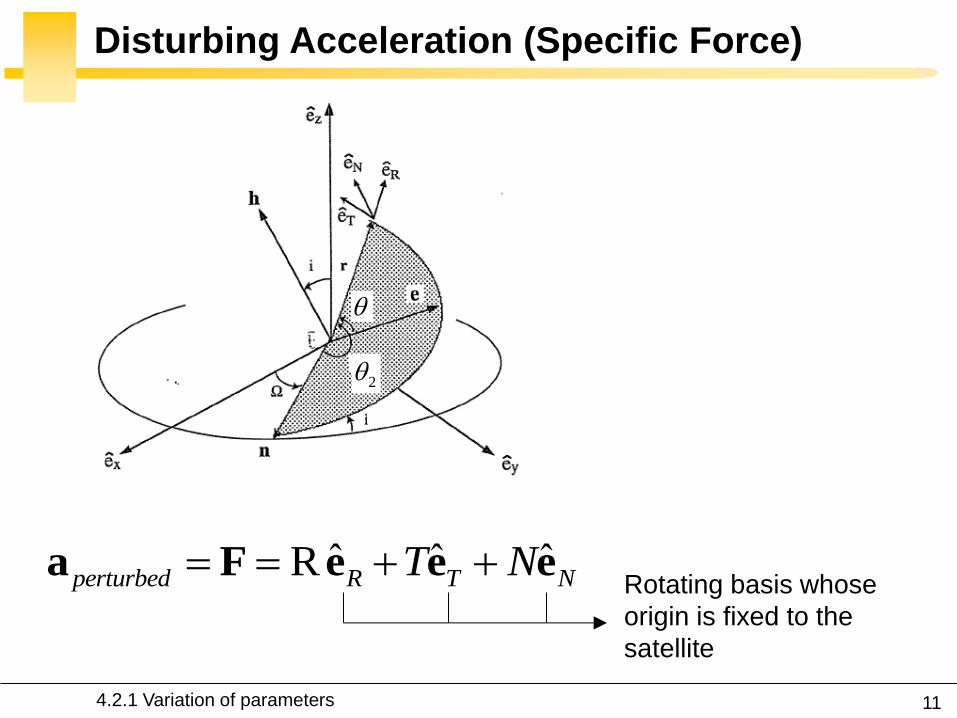
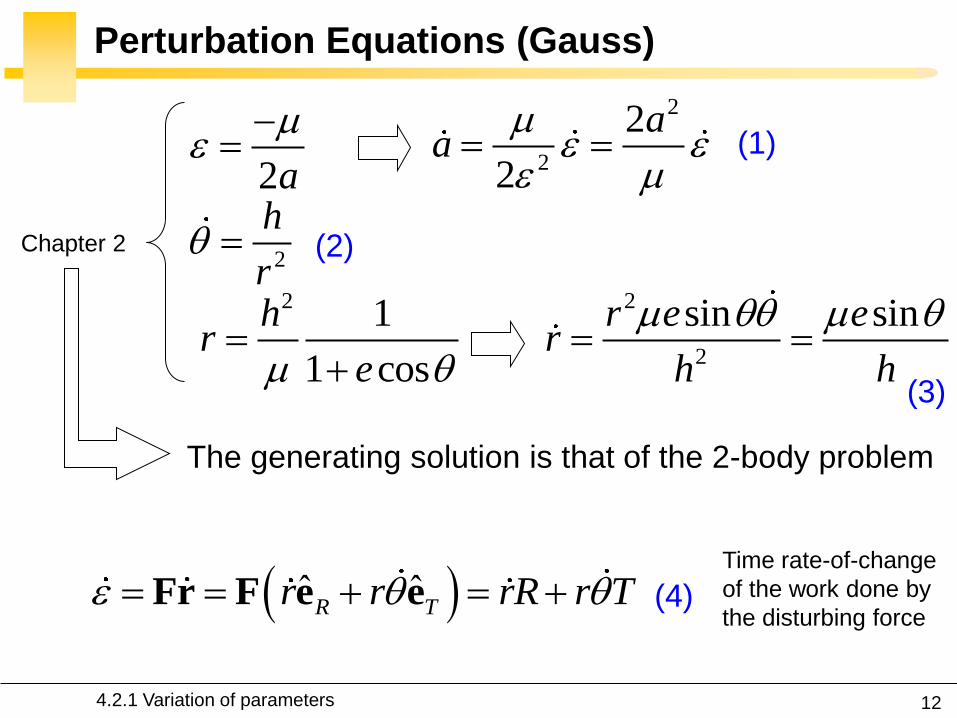
12
Perturbation Equations (Gauss)
421 Variation of parameters
2a
Chapter 2
2
2
2
2
aa
2
h
r
2 2
2
1 sin sin
1 cos
h r e er r
e h h
(1)
(2)
(3)
The generating solution is that of the 2-body problem
ˆ ˆR Tr r rR r T Fr F e e (4)
Time rate-of-change
of the work done by
the disturbing force
13
Perturbation Equations (Gauss)
421 Variation of parameters
(1)
(2)
(3)
(4)
2 2 2
2
2 sin 2sin
2 sin 1 cos
a e h a ha R T e R T
h r h r
aRe T e
h
2(1 )h a e
3
22 sin 1 cos
1
aa Re T e
e
Chapter 2
14
Perturbation Equations (Gauss)
3
22 Resin 1 cos
1
aa T e
e
2(1 )
sin cos cosa e
e R T E
2
2cos(1 )
1 cos
Na ei
e
JE Prussing BA Conway Orbital Mechanics Oxford University Press
421 Variation of parameters
2 sin 2 cos1 (1 )cos cos
1 cos
T ea ei R
e e
2 2(1 ) 2 cos cos sin 2 cos with
1 cos
e R e e T eaM nt
e e
2
2sin(1 )
sin 1 cos
Na e
i e
15
Perturbation Equations (Gauss)
Limited to eccentricities less than 1
Singular for e=0 sin i=0 (use of equinoctial elements)
In what follows we apply the Gauss equations to Earth
oblateness and drag Analytical expressions for third-body
and solar radiation forces are far less common because
their effects are much smaller for many orbits
421 Variation of parameters
16
Non-spherical Earth J2
Focus on the oblateness through the first zonal harmonic
J2 (tesseral and sectorial coefficients ignored)
The J2 effect can still be viewed a small perturbation when
compared to the attraction of the spherical Earth
422 Non-spherical Earth
17
Disturbing Acceleration (Specific Force)
2 2 222
4
3 1 3sin sinsin sin cos sin sin cos
2r T N
J R ii i i
r
F e e e
422 Non-spherical Earth
2 2
2
3sin 11
2
satRU J
r r
1 1 ˆˆ ˆ with cos
Ur r r
F r φ λ
Chapter 4A
18
Physical Interpretation of the Perturbation
The oblateness means that the force of gravity is no longer
within the orbital plane non-planar motion will result
The equatorial bulge exerts a force that pulls the satellite
back to the equatorial plane and thus tries to align the
orbital plane with the equator
Due to its angular momentum the orbit behaves like a
spinning top and reacts with a precessional motion of the
orbital plane (the orbital plane of the satellite to rotate in
inertial space)
422 Non-spherical Earth
19
Physical Interpretation of the Perturbation
422 Non-spherical Earth
20
Effect of Perturbations on Orbital Elements
Secular rate of change average rate of change over many
orbits
Periodic rate of change rate of change within one orbit
(J2 ~ 8-10km with a period equal to the orbital period)
422 Non-spherical Earth
21
Effect of Perturbations on Orbital Elements
Periodic
Secular
422 Non-spherical Earth
22
Secular Effects on Orbital Elements
Nodal regression regression of the nodal line
Apsidal rotation rotation of the apse line
Mean anomaly
No secular variations for a e i
422 Non-spherical Earth
2
2
2 2 7 20
1 3cos
2 (1 )
T
avg
J Rdt i
T e a
2
22
2 2 7 20
1 34 5sin
4 (1 )
T
avg
J Rdt i
T e a
23
Secular Effects Node Line
2
2
2 2 7 20
1 3cos
2 (1 )
T
avg
J Rdt i
T e a
For posigrade orbits the node line drifts westward
(regression of the nodes) And conversely
0 90 0i
For polar orbits the node line is stationary
90 0i
422 Non-spherical Earth
Vallado Fundamental of
Astrodynamics and
Applications Kluwer 2001
25
Exploitation Sun-Synchronous Orbits
The orbital plane makes a constant angle with the radial
from the sun
422 Non-spherical Earth
26
Exploitation Sun-Synchronous Orbits
The orbital plane must rotate in inertial space with the
angular velocity of the Earth in its orbit around the Sun
360ordm per 36526 days or 09856ordm per day
The satellite sees any given swath of the planet under
nearly the same condition of daylight or darkness day after
day
422 Non-spherical Earth
27
Existing Satellites
SPOT-5
(820 kms 987ordm)
NOAAPOES
(833 kms 987ordm)
28
Secular Effects Apse Line
2
22
2 2 7 20
1 34 5sin
4 (1 )
T
avg
J Rdt i
T e a
The perigee advances in the direction of the motion
of the satellite And conversely
0 634 or 1166 180 0i i
The apse line does not move
634 or 1166 0i i
422 Non-spherical Earth
Vallado Fundamental of
Astrodynamics and
Applications Kluwer 2001
30
Exploitation Molniya Orbits
A geostationary satellite cannot view effectively the far
northern latitudes into which Russian territory extends
(+ costly plane change maneuver for the launch vehicle )
Molniya telecommunications satellites are launched from
Plesetsk (628ordmN) into 63ordm inclination orbits having a
period of 12 hours
3
2 the apse line is 53000km longellip
aT
422 Non-spherical Earth
31
Analytic Propagators in STK 2-body J2
2-body constant orbital elements
J2 accounts for secular variations in the orbit elements
due to Earth oblateness periodic variations are
neglected
423 J2 propagator in STK
32
J2 Propagator Underlying Equations
423 J2 propagator in STK
33
2-body and J2 Propagators Applied to ISS
Two-body propagator J2 propagator
423 J2 propagator in STK
34
HPOP and J2 Propagators Applied to ISS
Nodal regression of the ISS
35
Effects of Atmospheric Drag Semi-Major Axis
2a
Lecture 2
2
2
2
2
aa
gt0
Because drag causes the dissipation of mechanical energy
from the system the semimajor axis contracts
424 Atmospheric drag
Drag paradox the effect of atmospheric drag is to increase
the satellite speed and kinetic energy
36
Effects of Atmospheric Drag Semi-Major Axis
21 10
2 2D r D
A AN R T C v C
m m a
0D
Aa a C
m
2
Df i f i
C Aa a t t
m
is assumed constant
424 Atmospheric drag
3
22 Resin 1 cos
1
aa T e
e
Circular orbit
37
Effects of Atmospheric Drag Orbit Plane
2
2sin(1 )
sin 1 cos
Na e
i e
2
2cos(1 )
1 cos
Na ei
e
The orientation of the orbit plane is not changed by drag
424 Atmospheric drag
38
Effects of Atmospheric Drag Apogee Perigee
Apogee height changes drastically perigee height remains
relatively constant
424 Atmospheric drag
Vallado Fundamental of Astrodynamics and Applications Kluwer 2001
39
Effects of Atmospheric Drag Eccentricity
Vallado Fundamental of Astrodynamics and Applications Kluwer 2001
424 Atmospheric drag
40
Early Reentry of Skylab (1979)
Increased solar activity which
increased drag on Skylab led to
an early reentry
Earth reentry footprint could not
be accurately predicted (due to
tumbling and other parameters)
Debris was found around
Esperance (31ndash34degS 122ndash
126degE) The Shire of Esperance
fined the United States $400 for
littering a fine which to this day
remains unpaid
424 Atmospheric drag
41
Lost of ASCA Satellite (2000)
July 15 2000 a strong solar
flare heated the Earthrsquos
atmosphere increasing the
air density to a value 100
times greater than that for
which its ADCS had been
designed to cope The
magnetorquers were unable
to compensate and the
satellite was lost
httpheasarcgsfcnasagovdocsascasafemodehtml
424 Atmospheric drag
42
Effects of Third-Body Perturbations
The only secular perturbations are in the node and in the
perigee
For near-Earth orbits the dominance of the oblateness
dictates that the orbital plane regresses about the polar
axis For higher orbits the regression will be about some
mean pole lying between the Earthrsquos pole and the ecliptic
pole
Many geosynchronous satellites launched 30 years ago
now have inclinations of up to plusmn15ordm collision avoidance
as the satellites drift back through the GEO belt
425 Third-body perturbations
43
Effects of Third-Body Perturbations
Vallado Fundamental of Astrodynamics and Applications Kluwer 2001
The Sunrsquos attraction
tends to turn the
satellite ring into the
ecliptic The orbit
precesses about the
pole of the ecliptic
425 Third-body perturbations
44
STK Analytic Propagator (SGP4)
The J2 propagator does not include drag
SGP4 which stands for Simplified General Perturbations
Satellite Orbit Model 4 is a NASANORAD algorithm
426 SGP4 propagator in STK
45
STK Analytic Propagator (SGP4)
Several assumptions propagation valid for short durations
(3-10 days)
TLE data should be used as the input (see Lecture 03)
It considers secular and periodic variations due to Earth
oblateness solar and lunar gravitational effects and
orbital decay using a drag model
426 SGP4 propagator in STK
46
SGP4 Applied to ISS RAAN
426 SGP4 propagator in STK
47
SGP4 Applied to ISS Semi-Major Axis
426 SGP4 propagator in STK
48
Further Reading on the Web Site
426 SGP4 propagator in STK
49
Effects of Solar Radiation Pressure
The effects are usually small for most satellites
Satellites with very low mass and large surface area are
more affected
427 Solar radiation pressure
Vallado Fundamental of
Astrodynamics and
Applications Kluwer
2001
51
Secular Effects Orders of Magnitude
Vallado Fundamental of Astrodynamics and Applications Kluwer 2001
52
Periodic Effects Orders of Magnitude
Vallado Fundamental of Astrodynamics and Applications Kluwer 2001
53
4 Non-Keplerian Motion
2
2
(1 )
sin
sin 1 cos
a e
N
i e
43 Numerical methods
431 Orbit prediction
432 Numerical integration
433 Single-step methods Runge-Kutta
434 Multi-step methods
435 Integrator and step size selection
436 ISS example
nt 1nt
r
54
2-body analytic propagator (constant orbital elements)
J2 analytic propagator (secular variations in the orbit
elements due to Earth oblateness
HPOP numerical integration of the equations of motion
(periodic and secular effects included)
STK Propagators
431 Orbit prediction
Accurate
Versatile
Errors accumulation
for long intervals
Computationally
intensive
55
Real-Life Example German Aerospace Agency
431 Orbit prediction
56
Real-Life Example German Aerospace Agency
57
Further Reading on the Web Site
431 Orbit prediction
58
Real-Life Example Envisat
httpnngesocesadeenvisat
ENVpredhtml
431 Orbit prediction
Why do the
predictions degrade
for lower altitudes
60
NASA began the first complex numerical integrations
during the late 1960s and early 1970s
Did you Know
1969 1968
431 Orbit prediction
61
What is Numerical Integration
1n nt t t
3 perturbedr
r r a
Given
Compute
( ) ( )n nt tr r
1 1( ) ( )n nt t r r
432 Numerical integration
62
State-Space Formulation
3 perturbedr
r r a
( )f tu u
ru
r
6-dimensional
state vector
432 Numerical integration
63
How to Perform Numerical Integration
2( )( ) ( ) ( ) ( ) ( )
2
ss
n n n n n s
h hf t h f t hf t f t f t R
s
Taylor series expansion
( )ntu
1( )nt u
432 Numerical integration
64
First-Order Taylor Approximation (Euler)
1
( ) ( ) ( )
( )
n n n
n n n n
t t t t t
t f t
u u u
u u uEuler step
0 1 2 3 4 5 60
5
10
15
20
25
30
35
40
Time t (s)
x(t
)=t2
Exact solution
The stepsize has to be extremely
small for accurate predictions
and it is necessary to develop
more effective algorithms
along the tangent
432 Numerical integration
65
Numerical Integration Methods
1 1 1
1 0
m m
n j n j j n j
j j
t
u u u
0 0
Implicit the solution method becomes
iterative in the nonlinear case
0 0 Explicit un+1 can be deduced directly from
the results at the previous time steps
=0
for 1
j j
j
Single-step the system at time tn+1
only depends on the previous state tn
State vector
0
for 1
j j
j
Multi-step the system at time tn+1 depends
several previous states tntn-1etc
432 Numerical integration
66
Examples Implicit vs Explicit
Trapezoidal rule (implicit)
nt 1nt
Euler forward (explicit)
nt 1nt
Euler backward (implicit)
nt 1nt
1n n nt u u u
1 1n n nt u u u
1
12
n n
n n t
u uu u
r
r
r
432 Numerical integration
67
A variety of methods has been applied in astrodynamics
Each of these methods has its own advantages and
drawbacks
Accuracy what is the order of the integration scheme
Efficiency how many function calls
Versatility can it be applied to a wide range of problems
Complexity is it easy to implement and use
Step size automatic step size control
Why Different Methods
431 Orbit prediction
68
Runge-Kutta Family Single-Step
Perhaps the most well-known numerical integrator
Difference with traditional Taylor series integrators the RK
family only requires the first derivative but several
evaluations are needed to move forward one step in time
Different variants explicit embedded etc
433 Single-step methods Runge-Kutta
69
Runge-Kutta Family Single-Step
with ( ) ( )t f tu u 0 0( )t u u
1
1
s
n n i i
i
t b
u u k
1 1
1
1
2
n n
i
i n ij j n i
j
f t c t
f t a t c t i s
k u
k u k
Slopes at
various points
within the
integration step
433 Single-step methods Runge-Kutta
70
Runge-Kutta Family Single-Step
Butcher Tableau
The Runge-Kutta methods are fully described by the
coefficients
c1
c2
cs
a21
as1
b1
as2
b2
ass-1
bs-1 hellip
hellip
hellip hellip hellip
bs
1
1
1
1
1
0
s
i
i
i
i ij
j
b
c
c a
433 Single-step methods Runge-Kutta
71
RK4 (Explicit)
1 2 3 41
2 2
6n n t
k k k ku u
Butcher Tableau
1
2 1
3 2
4 3
2 2
2 2
n n
n n
n n
n n
f t
t tf t
t tf t
f t t t
k u
k u k
k u k
k u k
433 Single-step methods Runge-Kutta
72
RK4 (Explicit)
1 2 3 41
2 2
6n n t
k k k ku u
1
2 1
3 2
4 3
2 2
2 2
n n
n n
n n
n n
f t
t tf t
t tf t
f t t t
k u
k u k
k u k
k u k
Slope at the beginning
Slope at the midpoint (k1 is
used to determine the value
of u Euler)
Slope at the midpoint (k2 is
now used)
Slope at the end
Estimated slope
(weighted average)
433 Single-step methods Runge-Kutta
73
RK4 (Explicit)
nt 2nt t nt t
1k3k
2k
4k
Estimate at new
time
u
433 Single-step methods Runge-Kutta
74
RK4 (Explicit)
The local truncation error for a 4th order RK is O(h5)
The accuracy is comparable to that of a 4th order Taylor
series but the Runge-Kutta method avoids the
calculation of higher-order derivatives
Easy to use and implement
The step size is fixed
433 Single-step methods Runge-Kutta
75
RK4 in STK
433 Single-step methods Runge-Kutta
76
Embedded Methods
They produce an estimate of the local truncation error
adjust the step size to keep local truncation errors
within some tolerances
This is done by having two methods in the tableau one with
order p and one with order p+1 with the same set of
function evaluations
( 1) ( 1) ( 1)
1
1
sp p p
n n i i
i
t b
u u k
( ) ( ) ( )
1
1
sp p p
n n i i
i
t b
u u k
433 Single-step methods Runge-Kutta
77
Embedded Methods
The two different approximations for the solution at each
step are compared
If the two answers are in close agreement the approximation is
accepted
If the two answers do not agree to a specified accuracy the step
size is reduced
If the answers agree to more significant digits than required the
step size is increased
433 Single-step methods Runge-Kutta
78
Ode45 in Matlab Simulink
Runge-Kutta (45) pair of Dormand and Prince
Variable step size
Matlab help This should be the first solver you try
433 Single-step methods Runge-Kutta
79
Ode45 in Matlab Simulink
edit ode45
433 Single-step methods Runge-Kutta
80
Ode45 in Matlab Simulink
Be very careful with the default parameters
options = odeset(RelTol1e-8AbsTol1e-8)
433 Single-step methods Runge-Kutta
81
RKF 7(8) Default Method in STK
Runge-Kutta-Fehlberg integration method of 7th order
with 8th order error control for the integration step size
433 Single-step methods Runge-Kutta
83
Multi-Step Methods (Predictor-Corrector)
They estimate the state over time using previously
determined back values of the solution
Unlike RK methods they only perform one evaluation for
each step forward but they usually have a predictor and a
corrector formula
Adams() ndash Bashforth - Moulton Gauss - Jackson
() The first with Le Verrier to predict the existence and position of Neptune
434 Multi-step methods
84
Multi-Step Methods Principle
( ) ( )t f tu u1
1( ) ( ) ( ) n
n
t
n nt
t t f t dt
u u u
unknown
Replace it by a
polynomial that
interpolates the
previous values Four function values
interpolated by a
third-order polynomial
t
u
434 Multi-step methods
85
Multi-Step Methods Initiation
with ( ) ( )t f tu u 0 0( )t u u
What is the inherent problem
t
u
434 Multi-step methods
86
Multi-Step Methods Initiation
Because these methods require back values they are not
self-starting
One may for instance use of a single-step method to
compute the first four values
434 Multi-step methods
87
Gauss-Jackson in STK
One of the most recommendable fixed-stepsize multistep
methods for orbit computations
88
Integrator Selection
435 Integrator and step size selection
Montenbruck and Gill
Satellite orbits Springer
2000
89
Integrator Selection
Pros
Very fast
Cons
Special starting procedure
Fixed time steps
Error control
Pros
Plug and play
Error control
Cons
Slower
Multi-step Single step
435 Integrator and step size selection
90
Why is the Step Size So Critical
Theoretical arguments
1 The accuracy and the stability of the algorithm are
directly related to the step size
2 Nonlinear equations of motion
Data for Landsat 4 and 6 in circular orbits around 800km
indicates that a one-minute step size yields about 47m
error
A three-minute step size produces about a 900m error
435 Integrator and step size selection
91
Why is the Step Size So Critical
More practical arguments
1 The computation time is directly related to the
step size
2 The particular choice of step size depends on the
most rapidly varying component in the disturbing
functions (eg 50 x 50 gravity field)
435 Integrator and step size selection
92
Appropriate Step Size
The problem of determining an appropriate step size is a
challenge in any numerical process
Fixed step size (rule of thumb for standard
applications)
But an algorithm with variable step size is really
helpful The step size is chosen in such a way that
each step contributes uniformly to the total integration
error
100
orbitTt
435 Integrator and step size selection
93
Three Examples XMM OUFTI-1 ISS
Can you plot the step size vs true anomaly
435 Integrator and step size selection
94
XMM Report in STK
435 Integrator and step size selection
95
XMM (e~08)
0 50 100 150 200 250 300 350 4000
1000
2000
3000
4000
5000
6000
True anomaly (deg)
Ste
p s
ize
(s)
435 Integrator and step size selection
96
ISS(e~0)
435 Integrator and step size selection
0 50 100 150 200 250 300 350 40030
35
40
45
50
55
60
65
70
True anomaly (deg)
Ste
p s
ize
(s)
97
ldquoDifficultrdquo Orbits
Automatic time step is especially nice on highly eccentric
orbits (Molniya XMM) These orbits are best computed
using variable step sizes to maintain some given level of
accuracy
Without this variable step size we waste a lot of time near
apoapsis when the integration is taking too small a step
Likewise the integrator may not be using a small enough step
size at periapsis where the satellite is traveling fast
435 Integrator and step size selection
98
HPOP Propagator ISS Example
1 Earthrsquos oblateness only
2 Drag only
3 Sun and moon only
4 SRP only
5 All together
436 ISS example
99
Earthrsquos Oblateness Only Ω
HPOP
J2
2-body
436 ISS example
100
Earthrsquos Oblateness Only i Ω a
HPOP with central body (20 + WGS84_EGM96)
(without dragSRPSun and Moon)
436 ISS example
101
Drag Only i Ω a
HPOP with drag ndash Harris Priester
(without oblatenessSRPSun and Moon)
436 ISS example
102
Drag Relationship with Eclipses
103
SRP Only i Ω a
HPOP with SRP
(without oblatenessdragSun and Moon)
436 ISS example
104
SRP Relationship with Eclipses
105
All Perturbations Together
436 ISS example
106
4 Non-Keplerian Motion
2
2
(1 )
sin
sin 1 cos
a e
N
i e
44 Geostationary satellites
107
Practical Example GEO Satellites
Nice illustration of
1 Perturbations of the 2-body problem
2 Secular and periodic contributions
3 Accuracy required by practical applications
4 The need for orbit correction and thrust forces
And it is a real-life example (telecommunications
meteorology)
44 GEO satellites
108
Three Main Perturbations for GEO Satellites
44 GEO satellites
1 Non-spherical Earth
2 SRP
3 Sun and Moon
109
Station Keeping of GEO Satellites
The effect of the perturbations is to cause the spacecraft
to drift away from its nominal station If the drift was
allowed to build up unchecked the spacecraft could
become useless
A station-keeping box is defined by a longitude and a
maximum authorized distance for satellite excursions in
longitude and latitude
For instance TC2 -8ordm plusmn 007ordm EW plusmn 005ordm NS
44 GEO satellites
110
East-West and North-South Drift
44 GEO satellites
NS drift
EW drift
What are the perturbations generating these drifts
111
East-West Drift
44 GEO satellites
A GEO satellite drifts in longitude due to the influence of
two main perturbations
1 The elliptic nature of the Earthrsquos equatorial cross-
section J22 (and not from the NS oblateness J2)
2
ΔV
ΔV vsat
vsat SRP
112
East-West Drift due to Equatorial Ellipticity
44 GEO satellites
113
East-West Drift due to Equatorial Ellipticity
44 GEO satellites
114
East-West Drift HPOP (20) vs HPOP (22)
44 GEO satellites
115
East-West Drift Stable Equilibirum
HPOP with 22
(without Sun and moonSRPdrag)
116
East-West Drift Stable Equilibirum
HPOP with 22
(without Sun and moonSRPdrag)
117
East-West Drift Stable Equilibirum
HPOP with 22
(without Sun and moonSRPdrag)
118
North-South Drift
The perturbations caused by the Sun and the Moon are
predominantly out-of-plane effects causing a change in
the inclination and in the right ascension of the orbit
ascending node
Similar effects on the orbit to those of the Earthrsquos
oblateness (but here with respect to the ecliptic)
A GEO satellite therefore drifts in latitude with a
fundamental period equal to the orbit period
119
North-South Drift
Period
HPOP with Sun and Moon
(without oblatenessSRPdrag)
120
North-South Drift
Period
HPOP with Sun and Moon
(without oblatenessSRPdrag)
121
Thrust Forces for Stationkeeping
GEO spacecraft require continual stationkeeping to stay
within the authorized box using onboard thrusters
44 GEO satellites
122
42 ANALYTIC TREATMENT
421 Variation of parameters
422 Non-spherical Earth
423 J2 propagator in STK
424 Atmospheric drag
425 Third-body perturbations
426 SGP4 propagator in STK
427 Solar radiation pressure
4 Non-Keplerian Motion
43 NUMERICAL METHODS
431 Orbit prediction
432 Numerical integration
433 Single-step methods Runge-Kutta
434 Multi-step methods
435 Integrator and step size selection
436 ISS example
44 GEOSTATIONARY SATELLITES
Gaeumltan Kerschen
Space Structures amp
Systems Lab (S3L)
4B Non-Keplerian Motion
Astrodynamics (AERO0024)
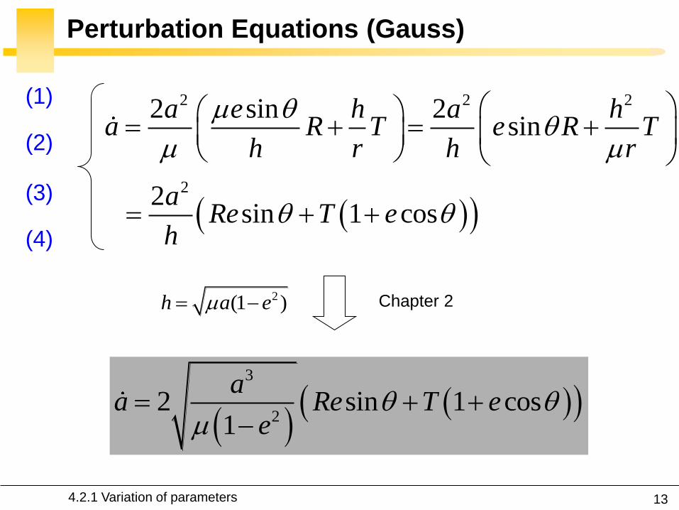
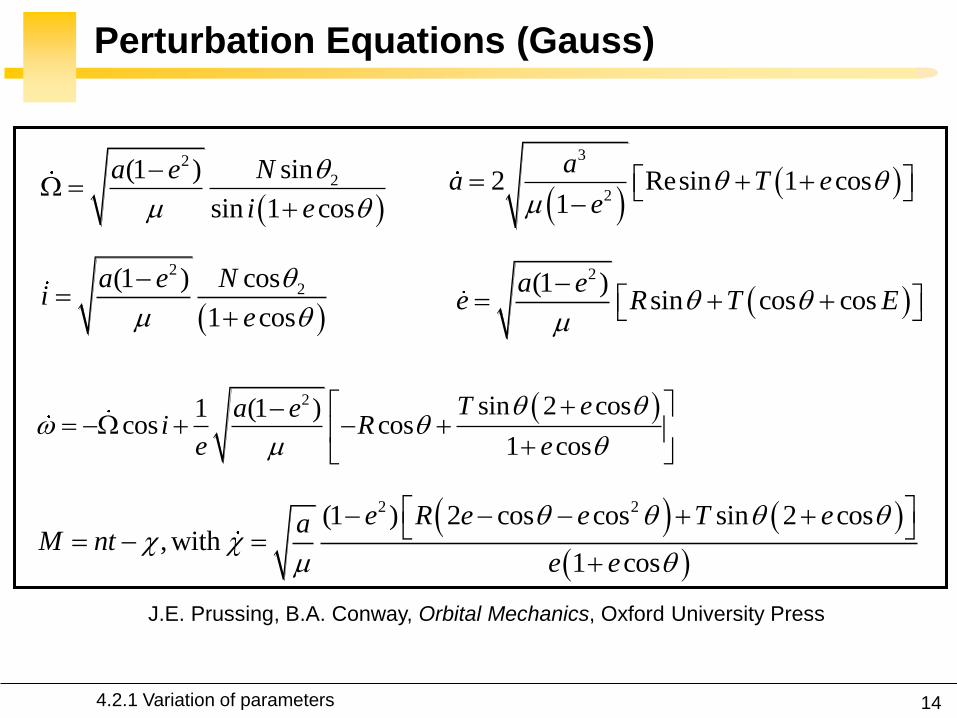

15
Perturbation Equations (Gauss)
Limited to eccentricities less than 1
Singular for e=0 sin i=0 (use of equinoctial elements)
In what follows we apply the Gauss equations to Earth
oblateness and drag Analytical expressions for third-body
and solar radiation forces are far less common because
their effects are much smaller for many orbits
421 Variation of parameters
16
Non-spherical Earth J2
Focus on the oblateness through the first zonal harmonic
J2 (tesseral and sectorial coefficients ignored)
The J2 effect can still be viewed a small perturbation when
compared to the attraction of the spherical Earth
422 Non-spherical Earth
17
Disturbing Acceleration (Specific Force)
2 2 222
4
3 1 3sin sinsin sin cos sin sin cos
2r T N
J R ii i i
r
F e e e
422 Non-spherical Earth
2 2
2
3sin 11
2
satRU J
r r
1 1 ˆˆ ˆ with cos
Ur r r
F r φ λ
Chapter 4A
18
Physical Interpretation of the Perturbation
The oblateness means that the force of gravity is no longer
within the orbital plane non-planar motion will result
The equatorial bulge exerts a force that pulls the satellite
back to the equatorial plane and thus tries to align the
orbital plane with the equator
Due to its angular momentum the orbit behaves like a
spinning top and reacts with a precessional motion of the
orbital plane (the orbital plane of the satellite to rotate in
inertial space)
422 Non-spherical Earth
19
Physical Interpretation of the Perturbation
422 Non-spherical Earth
20
Effect of Perturbations on Orbital Elements
Secular rate of change average rate of change over many
orbits
Periodic rate of change rate of change within one orbit
(J2 ~ 8-10km with a period equal to the orbital period)
422 Non-spherical Earth
21
Effect of Perturbations on Orbital Elements
Periodic
Secular
422 Non-spherical Earth
22
Secular Effects on Orbital Elements
Nodal regression regression of the nodal line
Apsidal rotation rotation of the apse line
Mean anomaly
No secular variations for a e i
422 Non-spherical Earth
2
2
2 2 7 20
1 3cos
2 (1 )
T
avg
J Rdt i
T e a
2
22
2 2 7 20
1 34 5sin
4 (1 )
T
avg
J Rdt i
T e a
23
Secular Effects Node Line
2
2
2 2 7 20
1 3cos
2 (1 )
T
avg
J Rdt i
T e a
For posigrade orbits the node line drifts westward
(regression of the nodes) And conversely
0 90 0i
For polar orbits the node line is stationary
90 0i
422 Non-spherical Earth
Vallado Fundamental of
Astrodynamics and
Applications Kluwer 2001
25
Exploitation Sun-Synchronous Orbits
The orbital plane makes a constant angle with the radial
from the sun
422 Non-spherical Earth
26
Exploitation Sun-Synchronous Orbits
The orbital plane must rotate in inertial space with the
angular velocity of the Earth in its orbit around the Sun
360ordm per 36526 days or 09856ordm per day
The satellite sees any given swath of the planet under
nearly the same condition of daylight or darkness day after
day
422 Non-spherical Earth
27
Existing Satellites
SPOT-5
(820 kms 987ordm)
NOAAPOES
(833 kms 987ordm)
28
Secular Effects Apse Line
2
22
2 2 7 20
1 34 5sin
4 (1 )
T
avg
J Rdt i
T e a
The perigee advances in the direction of the motion
of the satellite And conversely
0 634 or 1166 180 0i i
The apse line does not move
634 or 1166 0i i
422 Non-spherical Earth
Vallado Fundamental of
Astrodynamics and
Applications Kluwer 2001
30
Exploitation Molniya Orbits
A geostationary satellite cannot view effectively the far
northern latitudes into which Russian territory extends
(+ costly plane change maneuver for the launch vehicle )
Molniya telecommunications satellites are launched from
Plesetsk (628ordmN) into 63ordm inclination orbits having a
period of 12 hours
3
2 the apse line is 53000km longellip
aT
422 Non-spherical Earth
31
Analytic Propagators in STK 2-body J2
2-body constant orbital elements
J2 accounts for secular variations in the orbit elements
due to Earth oblateness periodic variations are
neglected
423 J2 propagator in STK
32
J2 Propagator Underlying Equations
423 J2 propagator in STK
33
2-body and J2 Propagators Applied to ISS
Two-body propagator J2 propagator
423 J2 propagator in STK
34
HPOP and J2 Propagators Applied to ISS
Nodal regression of the ISS
35
Effects of Atmospheric Drag Semi-Major Axis
2a
Lecture 2
2
2
2
2
aa
gt0
Because drag causes the dissipation of mechanical energy
from the system the semimajor axis contracts
424 Atmospheric drag
Drag paradox the effect of atmospheric drag is to increase
the satellite speed and kinetic energy
36
Effects of Atmospheric Drag Semi-Major Axis
21 10
2 2D r D
A AN R T C v C
m m a
0D
Aa a C
m
2
Df i f i
C Aa a t t
m
is assumed constant
424 Atmospheric drag
3
22 Resin 1 cos
1
aa T e
e
Circular orbit
37
Effects of Atmospheric Drag Orbit Plane
2
2sin(1 )
sin 1 cos
Na e
i e
2
2cos(1 )
1 cos
Na ei
e
The orientation of the orbit plane is not changed by drag
424 Atmospheric drag
38
Effects of Atmospheric Drag Apogee Perigee
Apogee height changes drastically perigee height remains
relatively constant
424 Atmospheric drag
Vallado Fundamental of Astrodynamics and Applications Kluwer 2001
39
Effects of Atmospheric Drag Eccentricity
Vallado Fundamental of Astrodynamics and Applications Kluwer 2001
424 Atmospheric drag
40
Early Reentry of Skylab (1979)
Increased solar activity which
increased drag on Skylab led to
an early reentry
Earth reentry footprint could not
be accurately predicted (due to
tumbling and other parameters)
Debris was found around
Esperance (31ndash34degS 122ndash
126degE) The Shire of Esperance
fined the United States $400 for
littering a fine which to this day
remains unpaid
424 Atmospheric drag
41
Lost of ASCA Satellite (2000)
July 15 2000 a strong solar
flare heated the Earthrsquos
atmosphere increasing the
air density to a value 100
times greater than that for
which its ADCS had been
designed to cope The
magnetorquers were unable
to compensate and the
satellite was lost
httpheasarcgsfcnasagovdocsascasafemodehtml
424 Atmospheric drag
42
Effects of Third-Body Perturbations
The only secular perturbations are in the node and in the
perigee
For near-Earth orbits the dominance of the oblateness
dictates that the orbital plane regresses about the polar
axis For higher orbits the regression will be about some
mean pole lying between the Earthrsquos pole and the ecliptic
pole
Many geosynchronous satellites launched 30 years ago
now have inclinations of up to plusmn15ordm collision avoidance
as the satellites drift back through the GEO belt
425 Third-body perturbations
43
Effects of Third-Body Perturbations
Vallado Fundamental of Astrodynamics and Applications Kluwer 2001
The Sunrsquos attraction
tends to turn the
satellite ring into the
ecliptic The orbit
precesses about the
pole of the ecliptic
425 Third-body perturbations
44
STK Analytic Propagator (SGP4)
The J2 propagator does not include drag
SGP4 which stands for Simplified General Perturbations
Satellite Orbit Model 4 is a NASANORAD algorithm
426 SGP4 propagator in STK
45
STK Analytic Propagator (SGP4)
Several assumptions propagation valid for short durations
(3-10 days)
TLE data should be used as the input (see Lecture 03)
It considers secular and periodic variations due to Earth
oblateness solar and lunar gravitational effects and
orbital decay using a drag model
426 SGP4 propagator in STK
46
SGP4 Applied to ISS RAAN
426 SGP4 propagator in STK
47
SGP4 Applied to ISS Semi-Major Axis
426 SGP4 propagator in STK
48
Further Reading on the Web Site
426 SGP4 propagator in STK
49
Effects of Solar Radiation Pressure
The effects are usually small for most satellites
Satellites with very low mass and large surface area are
more affected
427 Solar radiation pressure
Vallado Fundamental of
Astrodynamics and
Applications Kluwer
2001
51
Secular Effects Orders of Magnitude
Vallado Fundamental of Astrodynamics and Applications Kluwer 2001
52
Periodic Effects Orders of Magnitude
Vallado Fundamental of Astrodynamics and Applications Kluwer 2001
53
4 Non-Keplerian Motion
2
2
(1 )
sin
sin 1 cos
a e
N
i e
43 Numerical methods
431 Orbit prediction
432 Numerical integration
433 Single-step methods Runge-Kutta
434 Multi-step methods
435 Integrator and step size selection
436 ISS example
nt 1nt
r
54
2-body analytic propagator (constant orbital elements)
J2 analytic propagator (secular variations in the orbit
elements due to Earth oblateness
HPOP numerical integration of the equations of motion
(periodic and secular effects included)
STK Propagators
431 Orbit prediction
Accurate
Versatile
Errors accumulation
for long intervals
Computationally
intensive
55
Real-Life Example German Aerospace Agency
431 Orbit prediction
56
Real-Life Example German Aerospace Agency
57
Further Reading on the Web Site
431 Orbit prediction
58
Real-Life Example Envisat
httpnngesocesadeenvisat
ENVpredhtml
431 Orbit prediction
Why do the
predictions degrade
for lower altitudes
60
NASA began the first complex numerical integrations
during the late 1960s and early 1970s
Did you Know
1969 1968
431 Orbit prediction
61
What is Numerical Integration
1n nt t t
3 perturbedr
r r a
Given
Compute
( ) ( )n nt tr r
1 1( ) ( )n nt t r r
432 Numerical integration
62
State-Space Formulation
3 perturbedr
r r a
( )f tu u
ru
r
6-dimensional
state vector
432 Numerical integration
63
How to Perform Numerical Integration
2( )( ) ( ) ( ) ( ) ( )
2
ss
n n n n n s
h hf t h f t hf t f t f t R
s
Taylor series expansion
( )ntu
1( )nt u
432 Numerical integration
64
First-Order Taylor Approximation (Euler)
1
( ) ( ) ( )
( )
n n n
n n n n
t t t t t
t f t
u u u
u u uEuler step
0 1 2 3 4 5 60
5
10
15
20
25
30
35
40
Time t (s)
x(t
)=t2
Exact solution
The stepsize has to be extremely
small for accurate predictions
and it is necessary to develop
more effective algorithms
along the tangent
432 Numerical integration
65
Numerical Integration Methods
1 1 1
1 0
m m
n j n j j n j
j j
t
u u u
0 0
Implicit the solution method becomes
iterative in the nonlinear case
0 0 Explicit un+1 can be deduced directly from
the results at the previous time steps
=0
for 1
j j
j
Single-step the system at time tn+1
only depends on the previous state tn
State vector
0
for 1
j j
j
Multi-step the system at time tn+1 depends
several previous states tntn-1etc
432 Numerical integration
66
Examples Implicit vs Explicit
Trapezoidal rule (implicit)
nt 1nt
Euler forward (explicit)
nt 1nt
Euler backward (implicit)
nt 1nt
1n n nt u u u
1 1n n nt u u u
1
12
n n
n n t
u uu u
r
r
r
432 Numerical integration
67
A variety of methods has been applied in astrodynamics
Each of these methods has its own advantages and
drawbacks
Accuracy what is the order of the integration scheme
Efficiency how many function calls
Versatility can it be applied to a wide range of problems
Complexity is it easy to implement and use
Step size automatic step size control
Why Different Methods
431 Orbit prediction
68
Runge-Kutta Family Single-Step
Perhaps the most well-known numerical integrator
Difference with traditional Taylor series integrators the RK
family only requires the first derivative but several
evaluations are needed to move forward one step in time
Different variants explicit embedded etc
433 Single-step methods Runge-Kutta
69
Runge-Kutta Family Single-Step
with ( ) ( )t f tu u 0 0( )t u u
1
1
s
n n i i
i
t b
u u k
1 1
1
1
2
n n
i
i n ij j n i
j
f t c t
f t a t c t i s
k u
k u k
Slopes at
various points
within the
integration step
433 Single-step methods Runge-Kutta
70
Runge-Kutta Family Single-Step
Butcher Tableau
The Runge-Kutta methods are fully described by the
coefficients
c1
c2
cs
a21
as1
b1
as2
b2
ass-1
bs-1 hellip
hellip
hellip hellip hellip
bs
1
1
1
1
1
0
s
i
i
i
i ij
j
b
c
c a
433 Single-step methods Runge-Kutta
71
RK4 (Explicit)
1 2 3 41
2 2
6n n t
k k k ku u
Butcher Tableau
1
2 1
3 2
4 3
2 2
2 2
n n
n n
n n
n n
f t
t tf t
t tf t
f t t t
k u
k u k
k u k
k u k
433 Single-step methods Runge-Kutta
72
RK4 (Explicit)
1 2 3 41
2 2
6n n t
k k k ku u
1
2 1
3 2
4 3
2 2
2 2
n n
n n
n n
n n
f t
t tf t
t tf t
f t t t
k u
k u k
k u k
k u k
Slope at the beginning
Slope at the midpoint (k1 is
used to determine the value
of u Euler)
Slope at the midpoint (k2 is
now used)
Slope at the end
Estimated slope
(weighted average)
433 Single-step methods Runge-Kutta
73
RK4 (Explicit)
nt 2nt t nt t
1k3k
2k
4k
Estimate at new
time
u
433 Single-step methods Runge-Kutta
74
RK4 (Explicit)
The local truncation error for a 4th order RK is O(h5)
The accuracy is comparable to that of a 4th order Taylor
series but the Runge-Kutta method avoids the
calculation of higher-order derivatives
Easy to use and implement
The step size is fixed
433 Single-step methods Runge-Kutta
75
RK4 in STK
433 Single-step methods Runge-Kutta
76
Embedded Methods
They produce an estimate of the local truncation error
adjust the step size to keep local truncation errors
within some tolerances
This is done by having two methods in the tableau one with
order p and one with order p+1 with the same set of
function evaluations
( 1) ( 1) ( 1)
1
1
sp p p
n n i i
i
t b
u u k
( ) ( ) ( )
1
1
sp p p
n n i i
i
t b
u u k
433 Single-step methods Runge-Kutta
77
Embedded Methods
The two different approximations for the solution at each
step are compared
If the two answers are in close agreement the approximation is
accepted
If the two answers do not agree to a specified accuracy the step
size is reduced
If the answers agree to more significant digits than required the
step size is increased
433 Single-step methods Runge-Kutta
78
Ode45 in Matlab Simulink
Runge-Kutta (45) pair of Dormand and Prince
Variable step size
Matlab help This should be the first solver you try
433 Single-step methods Runge-Kutta
79
Ode45 in Matlab Simulink
edit ode45
433 Single-step methods Runge-Kutta
80
Ode45 in Matlab Simulink
Be very careful with the default parameters
options = odeset(RelTol1e-8AbsTol1e-8)
433 Single-step methods Runge-Kutta
81
RKF 7(8) Default Method in STK
Runge-Kutta-Fehlberg integration method of 7th order
with 8th order error control for the integration step size
433 Single-step methods Runge-Kutta
83
Multi-Step Methods (Predictor-Corrector)
They estimate the state over time using previously
determined back values of the solution
Unlike RK methods they only perform one evaluation for
each step forward but they usually have a predictor and a
corrector formula
Adams() ndash Bashforth - Moulton Gauss - Jackson
() The first with Le Verrier to predict the existence and position of Neptune
434 Multi-step methods
84
Multi-Step Methods Principle
( ) ( )t f tu u1
1( ) ( ) ( ) n
n
t
n nt
t t f t dt
u u u
unknown
Replace it by a
polynomial that
interpolates the
previous values Four function values
interpolated by a
third-order polynomial
t
u
434 Multi-step methods
85
Multi-Step Methods Initiation
with ( ) ( )t f tu u 0 0( )t u u
What is the inherent problem
t
u
434 Multi-step methods
86
Multi-Step Methods Initiation
Because these methods require back values they are not
self-starting
One may for instance use of a single-step method to
compute the first four values
434 Multi-step methods
87
Gauss-Jackson in STK
One of the most recommendable fixed-stepsize multistep
methods for orbit computations
88
Integrator Selection
435 Integrator and step size selection
Montenbruck and Gill
Satellite orbits Springer
2000
89
Integrator Selection
Pros
Very fast
Cons
Special starting procedure
Fixed time steps
Error control
Pros
Plug and play
Error control
Cons
Slower
Multi-step Single step
435 Integrator and step size selection
90
Why is the Step Size So Critical
Theoretical arguments
1 The accuracy and the stability of the algorithm are
directly related to the step size
2 Nonlinear equations of motion
Data for Landsat 4 and 6 in circular orbits around 800km
indicates that a one-minute step size yields about 47m
error
A three-minute step size produces about a 900m error
435 Integrator and step size selection
91
Why is the Step Size So Critical
More practical arguments
1 The computation time is directly related to the
step size
2 The particular choice of step size depends on the
most rapidly varying component in the disturbing
functions (eg 50 x 50 gravity field)
435 Integrator and step size selection
92
Appropriate Step Size
The problem of determining an appropriate step size is a
challenge in any numerical process
Fixed step size (rule of thumb for standard
applications)
But an algorithm with variable step size is really
helpful The step size is chosen in such a way that
each step contributes uniformly to the total integration
error
100
orbitTt
435 Integrator and step size selection
93
Three Examples XMM OUFTI-1 ISS
Can you plot the step size vs true anomaly
435 Integrator and step size selection
94
XMM Report in STK
435 Integrator and step size selection
95
XMM (e~08)
0 50 100 150 200 250 300 350 4000
1000
2000
3000
4000
5000
6000
True anomaly (deg)
Ste
p s
ize
(s)
435 Integrator and step size selection
96
ISS(e~0)
435 Integrator and step size selection
0 50 100 150 200 250 300 350 40030
35
40
45
50
55
60
65
70
True anomaly (deg)
Ste
p s
ize
(s)
97
ldquoDifficultrdquo Orbits
Automatic time step is especially nice on highly eccentric
orbits (Molniya XMM) These orbits are best computed
using variable step sizes to maintain some given level of
accuracy
Without this variable step size we waste a lot of time near
apoapsis when the integration is taking too small a step
Likewise the integrator may not be using a small enough step
size at periapsis where the satellite is traveling fast
435 Integrator and step size selection
98
HPOP Propagator ISS Example
1 Earthrsquos oblateness only
2 Drag only
3 Sun and moon only
4 SRP only
5 All together
436 ISS example
99
Earthrsquos Oblateness Only Ω
HPOP
J2
2-body
436 ISS example
100
Earthrsquos Oblateness Only i Ω a
HPOP with central body (20 + WGS84_EGM96)
(without dragSRPSun and Moon)
436 ISS example
101
Drag Only i Ω a
HPOP with drag ndash Harris Priester
(without oblatenessSRPSun and Moon)
436 ISS example
102
Drag Relationship with Eclipses
103
SRP Only i Ω a
HPOP with SRP
(without oblatenessdragSun and Moon)
436 ISS example
104
SRP Relationship with Eclipses
105
All Perturbations Together
436 ISS example
106
4 Non-Keplerian Motion
2
2
(1 )
sin
sin 1 cos
a e
N
i e
44 Geostationary satellites
107
Practical Example GEO Satellites
Nice illustration of
1 Perturbations of the 2-body problem
2 Secular and periodic contributions
3 Accuracy required by practical applications
4 The need for orbit correction and thrust forces
And it is a real-life example (telecommunications
meteorology)
44 GEO satellites
108
Three Main Perturbations for GEO Satellites
44 GEO satellites
1 Non-spherical Earth
2 SRP
3 Sun and Moon
109
Station Keeping of GEO Satellites
The effect of the perturbations is to cause the spacecraft
to drift away from its nominal station If the drift was
allowed to build up unchecked the spacecraft could
become useless
A station-keeping box is defined by a longitude and a
maximum authorized distance for satellite excursions in
longitude and latitude
For instance TC2 -8ordm plusmn 007ordm EW plusmn 005ordm NS
44 GEO satellites
110
East-West and North-South Drift
44 GEO satellites
NS drift
EW drift
What are the perturbations generating these drifts
111
East-West Drift
44 GEO satellites
A GEO satellite drifts in longitude due to the influence of
two main perturbations
1 The elliptic nature of the Earthrsquos equatorial cross-
section J22 (and not from the NS oblateness J2)
2
ΔV
ΔV vsat
vsat SRP
112
East-West Drift due to Equatorial Ellipticity
44 GEO satellites
113
East-West Drift due to Equatorial Ellipticity
44 GEO satellites
114
East-West Drift HPOP (20) vs HPOP (22)
44 GEO satellites
115
East-West Drift Stable Equilibirum
HPOP with 22
(without Sun and moonSRPdrag)
116
East-West Drift Stable Equilibirum
HPOP with 22
(without Sun and moonSRPdrag)
117
East-West Drift Stable Equilibirum
HPOP with 22
(without Sun and moonSRPdrag)
118
North-South Drift
The perturbations caused by the Sun and the Moon are
predominantly out-of-plane effects causing a change in
the inclination and in the right ascension of the orbit
ascending node
Similar effects on the orbit to those of the Earthrsquos
oblateness (but here with respect to the ecliptic)
A GEO satellite therefore drifts in latitude with a
fundamental period equal to the orbit period
119
North-South Drift
Period
HPOP with Sun and Moon
(without oblatenessSRPdrag)
120
North-South Drift
Period
HPOP with Sun and Moon
(without oblatenessSRPdrag)
121
Thrust Forces for Stationkeeping
GEO spacecraft require continual stationkeeping to stay
within the authorized box using onboard thrusters
44 GEO satellites
122
42 ANALYTIC TREATMENT
421 Variation of parameters
422 Non-spherical Earth
423 J2 propagator in STK
424 Atmospheric drag
425 Third-body perturbations
426 SGP4 propagator in STK
427 Solar radiation pressure
4 Non-Keplerian Motion
43 NUMERICAL METHODS
431 Orbit prediction
432 Numerical integration
433 Single-step methods Runge-Kutta
434 Multi-step methods
435 Integrator and step size selection
436 ISS example
44 GEOSTATIONARY SATELLITES
Gaeumltan Kerschen
Space Structures amp
Systems Lab (S3L)
4B Non-Keplerian Motion
Astrodynamics (AERO0024)
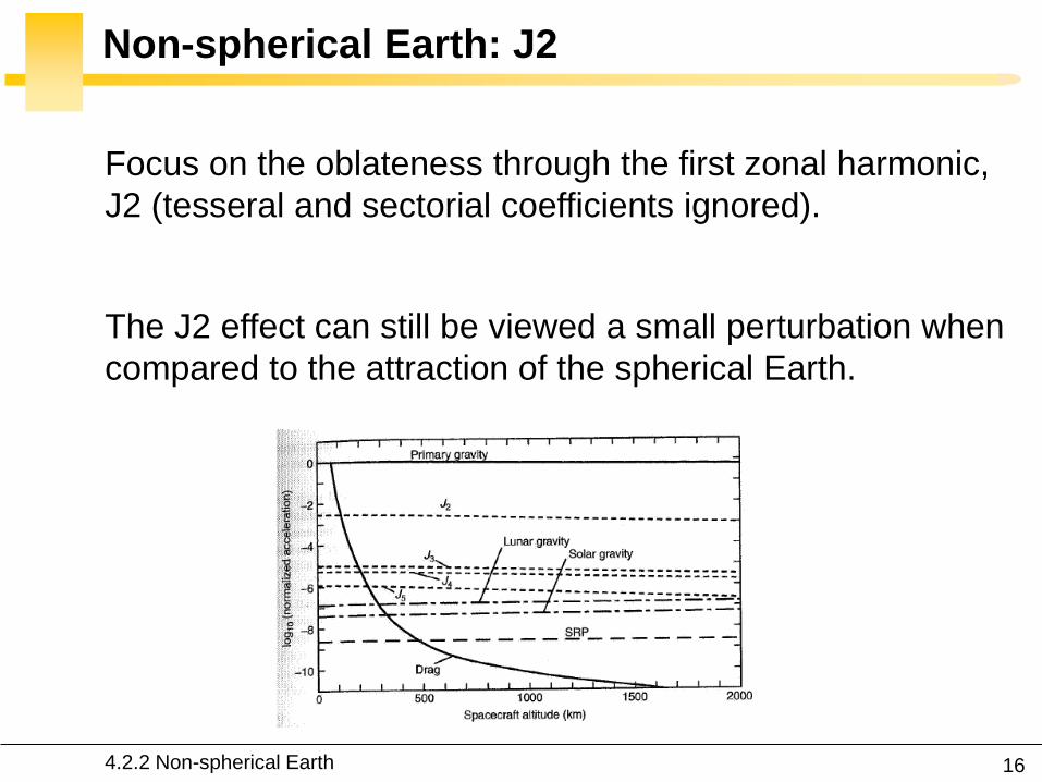
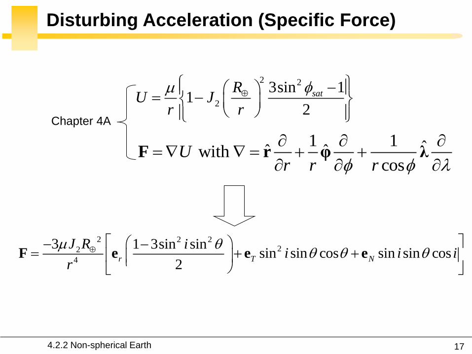
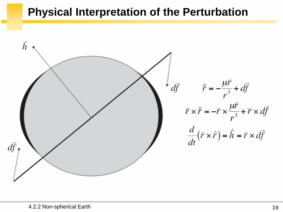
20
Effect of Perturbations on Orbital Elements
Secular rate of change average rate of change over many
orbits
Periodic rate of change rate of change within one orbit
(J2 ~ 8-10km with a period equal to the orbital period)
422 Non-spherical Earth
21
Effect of Perturbations on Orbital Elements
Periodic
Secular
422 Non-spherical Earth
22
Secular Effects on Orbital Elements
Nodal regression regression of the nodal line
Apsidal rotation rotation of the apse line
Mean anomaly
No secular variations for a e i
422 Non-spherical Earth
2
2
2 2 7 20
1 3cos
2 (1 )
T
avg
J Rdt i
T e a
2
22
2 2 7 20
1 34 5sin
4 (1 )
T
avg
J Rdt i
T e a
23
Secular Effects Node Line
2
2
2 2 7 20
1 3cos
2 (1 )
T
avg
J Rdt i
T e a
For posigrade orbits the node line drifts westward
(regression of the nodes) And conversely
0 90 0i
For polar orbits the node line is stationary
90 0i
422 Non-spherical Earth
Vallado Fundamental of
Astrodynamics and
Applications Kluwer 2001
25
Exploitation Sun-Synchronous Orbits
The orbital plane makes a constant angle with the radial
from the sun
422 Non-spherical Earth
26
Exploitation Sun-Synchronous Orbits
The orbital plane must rotate in inertial space with the
angular velocity of the Earth in its orbit around the Sun
360ordm per 36526 days or 09856ordm per day
The satellite sees any given swath of the planet under
nearly the same condition of daylight or darkness day after
day
422 Non-spherical Earth
27
Existing Satellites
SPOT-5
(820 kms 987ordm)
NOAAPOES
(833 kms 987ordm)
28
Secular Effects Apse Line
2
22
2 2 7 20
1 34 5sin
4 (1 )
T
avg
J Rdt i
T e a
The perigee advances in the direction of the motion
of the satellite And conversely
0 634 or 1166 180 0i i
The apse line does not move
634 or 1166 0i i
422 Non-spherical Earth
Vallado Fundamental of
Astrodynamics and
Applications Kluwer 2001
30
Exploitation Molniya Orbits
A geostationary satellite cannot view effectively the far
northern latitudes into which Russian territory extends
(+ costly plane change maneuver for the launch vehicle )
Molniya telecommunications satellites are launched from
Plesetsk (628ordmN) into 63ordm inclination orbits having a
period of 12 hours
3
2 the apse line is 53000km longellip
aT
422 Non-spherical Earth
31
Analytic Propagators in STK 2-body J2
2-body constant orbital elements
J2 accounts for secular variations in the orbit elements
due to Earth oblateness periodic variations are
neglected
423 J2 propagator in STK
32
J2 Propagator Underlying Equations
423 J2 propagator in STK
33
2-body and J2 Propagators Applied to ISS
Two-body propagator J2 propagator
423 J2 propagator in STK
34
HPOP and J2 Propagators Applied to ISS
Nodal regression of the ISS
35
Effects of Atmospheric Drag Semi-Major Axis
2a
Lecture 2
2
2
2
2
aa
gt0
Because drag causes the dissipation of mechanical energy
from the system the semimajor axis contracts
424 Atmospheric drag
Drag paradox the effect of atmospheric drag is to increase
the satellite speed and kinetic energy
36
Effects of Atmospheric Drag Semi-Major Axis
21 10
2 2D r D
A AN R T C v C
m m a
0D
Aa a C
m
2
Df i f i
C Aa a t t
m
is assumed constant
424 Atmospheric drag
3
22 Resin 1 cos
1
aa T e
e
Circular orbit
37
Effects of Atmospheric Drag Orbit Plane
2
2sin(1 )
sin 1 cos
Na e
i e
2
2cos(1 )
1 cos
Na ei
e
The orientation of the orbit plane is not changed by drag
424 Atmospheric drag
38
Effects of Atmospheric Drag Apogee Perigee
Apogee height changes drastically perigee height remains
relatively constant
424 Atmospheric drag
Vallado Fundamental of Astrodynamics and Applications Kluwer 2001
39
Effects of Atmospheric Drag Eccentricity
Vallado Fundamental of Astrodynamics and Applications Kluwer 2001
424 Atmospheric drag
40
Early Reentry of Skylab (1979)
Increased solar activity which
increased drag on Skylab led to
an early reentry
Earth reentry footprint could not
be accurately predicted (due to
tumbling and other parameters)
Debris was found around
Esperance (31ndash34degS 122ndash
126degE) The Shire of Esperance
fined the United States $400 for
littering a fine which to this day
remains unpaid
424 Atmospheric drag
41
Lost of ASCA Satellite (2000)
July 15 2000 a strong solar
flare heated the Earthrsquos
atmosphere increasing the
air density to a value 100
times greater than that for
which its ADCS had been
designed to cope The
magnetorquers were unable
to compensate and the
satellite was lost
httpheasarcgsfcnasagovdocsascasafemodehtml
424 Atmospheric drag
42
Effects of Third-Body Perturbations
The only secular perturbations are in the node and in the
perigee
For near-Earth orbits the dominance of the oblateness
dictates that the orbital plane regresses about the polar
axis For higher orbits the regression will be about some
mean pole lying between the Earthrsquos pole and the ecliptic
pole
Many geosynchronous satellites launched 30 years ago
now have inclinations of up to plusmn15ordm collision avoidance
as the satellites drift back through the GEO belt
425 Third-body perturbations
43
Effects of Third-Body Perturbations
Vallado Fundamental of Astrodynamics and Applications Kluwer 2001
The Sunrsquos attraction
tends to turn the
satellite ring into the
ecliptic The orbit
precesses about the
pole of the ecliptic
425 Third-body perturbations
44
STK Analytic Propagator (SGP4)
The J2 propagator does not include drag
SGP4 which stands for Simplified General Perturbations
Satellite Orbit Model 4 is a NASANORAD algorithm
426 SGP4 propagator in STK
45
STK Analytic Propagator (SGP4)
Several assumptions propagation valid for short durations
(3-10 days)
TLE data should be used as the input (see Lecture 03)
It considers secular and periodic variations due to Earth
oblateness solar and lunar gravitational effects and
orbital decay using a drag model
426 SGP4 propagator in STK
46
SGP4 Applied to ISS RAAN
426 SGP4 propagator in STK
47
SGP4 Applied to ISS Semi-Major Axis
426 SGP4 propagator in STK
48
Further Reading on the Web Site
426 SGP4 propagator in STK
49
Effects of Solar Radiation Pressure
The effects are usually small for most satellites
Satellites with very low mass and large surface area are
more affected
427 Solar radiation pressure
Vallado Fundamental of
Astrodynamics and
Applications Kluwer
2001
51
Secular Effects Orders of Magnitude
Vallado Fundamental of Astrodynamics and Applications Kluwer 2001
52
Periodic Effects Orders of Magnitude
Vallado Fundamental of Astrodynamics and Applications Kluwer 2001
53
4 Non-Keplerian Motion
2
2
(1 )
sin
sin 1 cos
a e
N
i e
43 Numerical methods
431 Orbit prediction
432 Numerical integration
433 Single-step methods Runge-Kutta
434 Multi-step methods
435 Integrator and step size selection
436 ISS example
nt 1nt
r
54
2-body analytic propagator (constant orbital elements)
J2 analytic propagator (secular variations in the orbit
elements due to Earth oblateness
HPOP numerical integration of the equations of motion
(periodic and secular effects included)
STK Propagators
431 Orbit prediction
Accurate
Versatile
Errors accumulation
for long intervals
Computationally
intensive
55
Real-Life Example German Aerospace Agency
431 Orbit prediction
56
Real-Life Example German Aerospace Agency
57
Further Reading on the Web Site
431 Orbit prediction
58
Real-Life Example Envisat
httpnngesocesadeenvisat
ENVpredhtml
431 Orbit prediction
Why do the
predictions degrade
for lower altitudes
60
NASA began the first complex numerical integrations
during the late 1960s and early 1970s
Did you Know
1969 1968
431 Orbit prediction
61
What is Numerical Integration
1n nt t t
3 perturbedr
r r a
Given
Compute
( ) ( )n nt tr r
1 1( ) ( )n nt t r r
432 Numerical integration
62
State-Space Formulation
3 perturbedr
r r a
( )f tu u
ru
r
6-dimensional
state vector
432 Numerical integration
63
How to Perform Numerical Integration
2( )( ) ( ) ( ) ( ) ( )
2
ss
n n n n n s
h hf t h f t hf t f t f t R
s
Taylor series expansion
( )ntu
1( )nt u
432 Numerical integration
64
First-Order Taylor Approximation (Euler)
1
( ) ( ) ( )
( )
n n n
n n n n
t t t t t
t f t
u u u
u u uEuler step
0 1 2 3 4 5 60
5
10
15
20
25
30
35
40
Time t (s)
x(t
)=t2
Exact solution
The stepsize has to be extremely
small for accurate predictions
and it is necessary to develop
more effective algorithms
along the tangent
432 Numerical integration
65
Numerical Integration Methods
1 1 1
1 0
m m
n j n j j n j
j j
t
u u u
0 0
Implicit the solution method becomes
iterative in the nonlinear case
0 0 Explicit un+1 can be deduced directly from
the results at the previous time steps
=0
for 1
j j
j
Single-step the system at time tn+1
only depends on the previous state tn
State vector
0
for 1
j j
j
Multi-step the system at time tn+1 depends
several previous states tntn-1etc
432 Numerical integration
66
Examples Implicit vs Explicit
Trapezoidal rule (implicit)
nt 1nt
Euler forward (explicit)
nt 1nt
Euler backward (implicit)
nt 1nt
1n n nt u u u
1 1n n nt u u u
1
12
n n
n n t
u uu u
r
r
r
432 Numerical integration
67
A variety of methods has been applied in astrodynamics
Each of these methods has its own advantages and
drawbacks
Accuracy what is the order of the integration scheme
Efficiency how many function calls
Versatility can it be applied to a wide range of problems
Complexity is it easy to implement and use
Step size automatic step size control
Why Different Methods
431 Orbit prediction
68
Runge-Kutta Family Single-Step
Perhaps the most well-known numerical integrator
Difference with traditional Taylor series integrators the RK
family only requires the first derivative but several
evaluations are needed to move forward one step in time
Different variants explicit embedded etc
433 Single-step methods Runge-Kutta
69
Runge-Kutta Family Single-Step
with ( ) ( )t f tu u 0 0( )t u u
1
1
s
n n i i
i
t b
u u k
1 1
1
1
2
n n
i
i n ij j n i
j
f t c t
f t a t c t i s
k u
k u k
Slopes at
various points
within the
integration step
433 Single-step methods Runge-Kutta
70
Runge-Kutta Family Single-Step
Butcher Tableau
The Runge-Kutta methods are fully described by the
coefficients
c1
c2
cs
a21
as1
b1
as2
b2
ass-1
bs-1 hellip
hellip
hellip hellip hellip
bs
1
1
1
1
1
0
s
i
i
i
i ij
j
b
c
c a
433 Single-step methods Runge-Kutta
71
RK4 (Explicit)
1 2 3 41
2 2
6n n t
k k k ku u
Butcher Tableau
1
2 1
3 2
4 3
2 2
2 2
n n
n n
n n
n n
f t
t tf t
t tf t
f t t t
k u
k u k
k u k
k u k
433 Single-step methods Runge-Kutta
72
RK4 (Explicit)
1 2 3 41
2 2
6n n t
k k k ku u
1
2 1
3 2
4 3
2 2
2 2
n n
n n
n n
n n
f t
t tf t
t tf t
f t t t
k u
k u k
k u k
k u k
Slope at the beginning
Slope at the midpoint (k1 is
used to determine the value
of u Euler)
Slope at the midpoint (k2 is
now used)
Slope at the end
Estimated slope
(weighted average)
433 Single-step methods Runge-Kutta
73
RK4 (Explicit)
nt 2nt t nt t
1k3k
2k
4k
Estimate at new
time
u
433 Single-step methods Runge-Kutta
74
RK4 (Explicit)
The local truncation error for a 4th order RK is O(h5)
The accuracy is comparable to that of a 4th order Taylor
series but the Runge-Kutta method avoids the
calculation of higher-order derivatives
Easy to use and implement
The step size is fixed
433 Single-step methods Runge-Kutta
75
RK4 in STK
433 Single-step methods Runge-Kutta
76
Embedded Methods
They produce an estimate of the local truncation error
adjust the step size to keep local truncation errors
within some tolerances
This is done by having two methods in the tableau one with
order p and one with order p+1 with the same set of
function evaluations
( 1) ( 1) ( 1)
1
1
sp p p
n n i i
i
t b
u u k
( ) ( ) ( )
1
1
sp p p
n n i i
i
t b
u u k
433 Single-step methods Runge-Kutta
77
Embedded Methods
The two different approximations for the solution at each
step are compared
If the two answers are in close agreement the approximation is
accepted
If the two answers do not agree to a specified accuracy the step
size is reduced
If the answers agree to more significant digits than required the
step size is increased
433 Single-step methods Runge-Kutta
78
Ode45 in Matlab Simulink
Runge-Kutta (45) pair of Dormand and Prince
Variable step size
Matlab help This should be the first solver you try
433 Single-step methods Runge-Kutta
79
Ode45 in Matlab Simulink
edit ode45
433 Single-step methods Runge-Kutta
80
Ode45 in Matlab Simulink
Be very careful with the default parameters
options = odeset(RelTol1e-8AbsTol1e-8)
433 Single-step methods Runge-Kutta
81
RKF 7(8) Default Method in STK
Runge-Kutta-Fehlberg integration method of 7th order
with 8th order error control for the integration step size
433 Single-step methods Runge-Kutta
83
Multi-Step Methods (Predictor-Corrector)
They estimate the state over time using previously
determined back values of the solution
Unlike RK methods they only perform one evaluation for
each step forward but they usually have a predictor and a
corrector formula
Adams() ndash Bashforth - Moulton Gauss - Jackson
() The first with Le Verrier to predict the existence and position of Neptune
434 Multi-step methods
84
Multi-Step Methods Principle
( ) ( )t f tu u1
1( ) ( ) ( ) n
n
t
n nt
t t f t dt
u u u
unknown
Replace it by a
polynomial that
interpolates the
previous values Four function values
interpolated by a
third-order polynomial
t
u
434 Multi-step methods
85
Multi-Step Methods Initiation
with ( ) ( )t f tu u 0 0( )t u u
What is the inherent problem
t
u
434 Multi-step methods
86
Multi-Step Methods Initiation
Because these methods require back values they are not
self-starting
One may for instance use of a single-step method to
compute the first four values
434 Multi-step methods
87
Gauss-Jackson in STK
One of the most recommendable fixed-stepsize multistep
methods for orbit computations
88
Integrator Selection
435 Integrator and step size selection
Montenbruck and Gill
Satellite orbits Springer
2000
89
Integrator Selection
Pros
Very fast
Cons
Special starting procedure
Fixed time steps
Error control
Pros
Plug and play
Error control
Cons
Slower
Multi-step Single step
435 Integrator and step size selection
90
Why is the Step Size So Critical
Theoretical arguments
1 The accuracy and the stability of the algorithm are
directly related to the step size
2 Nonlinear equations of motion
Data for Landsat 4 and 6 in circular orbits around 800km
indicates that a one-minute step size yields about 47m
error
A three-minute step size produces about a 900m error
435 Integrator and step size selection
91
Why is the Step Size So Critical
More practical arguments
1 The computation time is directly related to the
step size
2 The particular choice of step size depends on the
most rapidly varying component in the disturbing
functions (eg 50 x 50 gravity field)
435 Integrator and step size selection
92
Appropriate Step Size
The problem of determining an appropriate step size is a
challenge in any numerical process
Fixed step size (rule of thumb for standard
applications)
But an algorithm with variable step size is really
helpful The step size is chosen in such a way that
each step contributes uniformly to the total integration
error
100
orbitTt
435 Integrator and step size selection
93
Three Examples XMM OUFTI-1 ISS
Can you plot the step size vs true anomaly
435 Integrator and step size selection
94
XMM Report in STK
435 Integrator and step size selection
95
XMM (e~08)
0 50 100 150 200 250 300 350 4000
1000
2000
3000
4000
5000
6000
True anomaly (deg)
Ste
p s
ize
(s)
435 Integrator and step size selection
96
ISS(e~0)
435 Integrator and step size selection
0 50 100 150 200 250 300 350 40030
35
40
45
50
55
60
65
70
True anomaly (deg)
Ste
p s
ize
(s)
97
ldquoDifficultrdquo Orbits
Automatic time step is especially nice on highly eccentric
orbits (Molniya XMM) These orbits are best computed
using variable step sizes to maintain some given level of
accuracy
Without this variable step size we waste a lot of time near
apoapsis when the integration is taking too small a step
Likewise the integrator may not be using a small enough step
size at periapsis where the satellite is traveling fast
435 Integrator and step size selection
98
HPOP Propagator ISS Example
1 Earthrsquos oblateness only
2 Drag only
3 Sun and moon only
4 SRP only
5 All together
436 ISS example
99
Earthrsquos Oblateness Only Ω
HPOP
J2
2-body
436 ISS example
100
Earthrsquos Oblateness Only i Ω a
HPOP with central body (20 + WGS84_EGM96)
(without dragSRPSun and Moon)
436 ISS example
101
Drag Only i Ω a
HPOP with drag ndash Harris Priester
(without oblatenessSRPSun and Moon)
436 ISS example
102
Drag Relationship with Eclipses
103
SRP Only i Ω a
HPOP with SRP
(without oblatenessdragSun and Moon)
436 ISS example
104
SRP Relationship with Eclipses
105
All Perturbations Together
436 ISS example
106
4 Non-Keplerian Motion
2
2
(1 )
sin
sin 1 cos
a e
N
i e
44 Geostationary satellites
107
Practical Example GEO Satellites
Nice illustration of
1 Perturbations of the 2-body problem
2 Secular and periodic contributions
3 Accuracy required by practical applications
4 The need for orbit correction and thrust forces
And it is a real-life example (telecommunications
meteorology)
44 GEO satellites
108
Three Main Perturbations for GEO Satellites
44 GEO satellites
1 Non-spherical Earth
2 SRP
3 Sun and Moon
109
Station Keeping of GEO Satellites
The effect of the perturbations is to cause the spacecraft
to drift away from its nominal station If the drift was
allowed to build up unchecked the spacecraft could
become useless
A station-keeping box is defined by a longitude and a
maximum authorized distance for satellite excursions in
longitude and latitude
For instance TC2 -8ordm plusmn 007ordm EW plusmn 005ordm NS
44 GEO satellites
110
East-West and North-South Drift
44 GEO satellites
NS drift
EW drift
What are the perturbations generating these drifts
111
East-West Drift
44 GEO satellites
A GEO satellite drifts in longitude due to the influence of
two main perturbations
1 The elliptic nature of the Earthrsquos equatorial cross-
section J22 (and not from the NS oblateness J2)
2
ΔV
ΔV vsat
vsat SRP
112
East-West Drift due to Equatorial Ellipticity
44 GEO satellites
113
East-West Drift due to Equatorial Ellipticity
44 GEO satellites
114
East-West Drift HPOP (20) vs HPOP (22)
44 GEO satellites
115
East-West Drift Stable Equilibirum
HPOP with 22
(without Sun and moonSRPdrag)
116
East-West Drift Stable Equilibirum
HPOP with 22
(without Sun and moonSRPdrag)
117
East-West Drift Stable Equilibirum
HPOP with 22
(without Sun and moonSRPdrag)
118
North-South Drift
The perturbations caused by the Sun and the Moon are
predominantly out-of-plane effects causing a change in
the inclination and in the right ascension of the orbit
ascending node
Similar effects on the orbit to those of the Earthrsquos
oblateness (but here with respect to the ecliptic)
A GEO satellite therefore drifts in latitude with a
fundamental period equal to the orbit period
119
North-South Drift
Period
HPOP with Sun and Moon
(without oblatenessSRPdrag)
120
North-South Drift
Period
HPOP with Sun and Moon
(without oblatenessSRPdrag)
121
Thrust Forces for Stationkeeping
GEO spacecraft require continual stationkeeping to stay
within the authorized box using onboard thrusters
44 GEO satellites
122
42 ANALYTIC TREATMENT
421 Variation of parameters
422 Non-spherical Earth
423 J2 propagator in STK
424 Atmospheric drag
425 Third-body perturbations
426 SGP4 propagator in STK
427 Solar radiation pressure
4 Non-Keplerian Motion
43 NUMERICAL METHODS
431 Orbit prediction
432 Numerical integration
433 Single-step methods Runge-Kutta
434 Multi-step methods
435 Integrator and step size selection
436 ISS example
44 GEOSTATIONARY SATELLITES
Gaeumltan Kerschen
Space Structures amp
Systems Lab (S3L)
4B Non-Keplerian Motion
Astrodynamics (AERO0024)
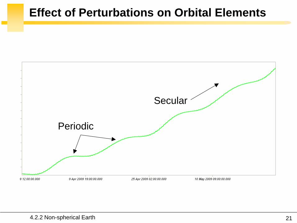
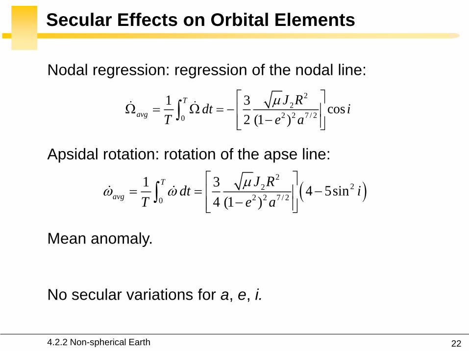
22
Secular Effects on Orbital Elements
Nodal regression regression of the nodal line
Apsidal rotation rotation of the apse line
Mean anomaly
No secular variations for a e i
422 Non-spherical Earth
2
2
2 2 7 20
1 3cos
2 (1 )
T
avg
J Rdt i
T e a
2
22
2 2 7 20
1 34 5sin
4 (1 )
T
avg
J Rdt i
T e a
23
Secular Effects Node Line
2
2
2 2 7 20
1 3cos
2 (1 )
T
avg
J Rdt i
T e a
For posigrade orbits the node line drifts westward
(regression of the nodes) And conversely
0 90 0i
For polar orbits the node line is stationary
90 0i
422 Non-spherical Earth
Vallado Fundamental of
Astrodynamics and
Applications Kluwer 2001
25
Exploitation Sun-Synchronous Orbits
The orbital plane makes a constant angle with the radial
from the sun
422 Non-spherical Earth
26
Exploitation Sun-Synchronous Orbits
The orbital plane must rotate in inertial space with the
angular velocity of the Earth in its orbit around the Sun
360ordm per 36526 days or 09856ordm per day
The satellite sees any given swath of the planet under
nearly the same condition of daylight or darkness day after
day
422 Non-spherical Earth
27
Existing Satellites
SPOT-5
(820 kms 987ordm)
NOAAPOES
(833 kms 987ordm)
28
Secular Effects Apse Line
2
22
2 2 7 20
1 34 5sin
4 (1 )
T
avg
J Rdt i
T e a
The perigee advances in the direction of the motion
of the satellite And conversely
0 634 or 1166 180 0i i
The apse line does not move
634 or 1166 0i i
422 Non-spherical Earth
Vallado Fundamental of
Astrodynamics and
Applications Kluwer 2001
30
Exploitation Molniya Orbits
A geostationary satellite cannot view effectively the far
northern latitudes into which Russian territory extends
(+ costly plane change maneuver for the launch vehicle )
Molniya telecommunications satellites are launched from
Plesetsk (628ordmN) into 63ordm inclination orbits having a
period of 12 hours
3
2 the apse line is 53000km longellip
aT
422 Non-spherical Earth
31
Analytic Propagators in STK 2-body J2
2-body constant orbital elements
J2 accounts for secular variations in the orbit elements
due to Earth oblateness periodic variations are
neglected
423 J2 propagator in STK
32
J2 Propagator Underlying Equations
423 J2 propagator in STK
33
2-body and J2 Propagators Applied to ISS
Two-body propagator J2 propagator
423 J2 propagator in STK
34
HPOP and J2 Propagators Applied to ISS
Nodal regression of the ISS
35
Effects of Atmospheric Drag Semi-Major Axis
2a
Lecture 2
2
2
2
2
aa
gt0
Because drag causes the dissipation of mechanical energy
from the system the semimajor axis contracts
424 Atmospheric drag
Drag paradox the effect of atmospheric drag is to increase
the satellite speed and kinetic energy
36
Effects of Atmospheric Drag Semi-Major Axis
21 10
2 2D r D
A AN R T C v C
m m a
0D
Aa a C
m
2
Df i f i
C Aa a t t
m
is assumed constant
424 Atmospheric drag
3
22 Resin 1 cos
1
aa T e
e
Circular orbit
37
Effects of Atmospheric Drag Orbit Plane
2
2sin(1 )
sin 1 cos
Na e
i e
2
2cos(1 )
1 cos
Na ei
e
The orientation of the orbit plane is not changed by drag
424 Atmospheric drag
38
Effects of Atmospheric Drag Apogee Perigee
Apogee height changes drastically perigee height remains
relatively constant
424 Atmospheric drag
Vallado Fundamental of Astrodynamics and Applications Kluwer 2001
39
Effects of Atmospheric Drag Eccentricity
Vallado Fundamental of Astrodynamics and Applications Kluwer 2001
424 Atmospheric drag
40
Early Reentry of Skylab (1979)
Increased solar activity which
increased drag on Skylab led to
an early reentry
Earth reentry footprint could not
be accurately predicted (due to
tumbling and other parameters)
Debris was found around
Esperance (31ndash34degS 122ndash
126degE) The Shire of Esperance
fined the United States $400 for
littering a fine which to this day
remains unpaid
424 Atmospheric drag
41
Lost of ASCA Satellite (2000)
July 15 2000 a strong solar
flare heated the Earthrsquos
atmosphere increasing the
air density to a value 100
times greater than that for
which its ADCS had been
designed to cope The
magnetorquers were unable
to compensate and the
satellite was lost
httpheasarcgsfcnasagovdocsascasafemodehtml
424 Atmospheric drag
42
Effects of Third-Body Perturbations
The only secular perturbations are in the node and in the
perigee
For near-Earth orbits the dominance of the oblateness
dictates that the orbital plane regresses about the polar
axis For higher orbits the regression will be about some
mean pole lying between the Earthrsquos pole and the ecliptic
pole
Many geosynchronous satellites launched 30 years ago
now have inclinations of up to plusmn15ordm collision avoidance
as the satellites drift back through the GEO belt
425 Third-body perturbations
43
Effects of Third-Body Perturbations
Vallado Fundamental of Astrodynamics and Applications Kluwer 2001
The Sunrsquos attraction
tends to turn the
satellite ring into the
ecliptic The orbit
precesses about the
pole of the ecliptic
425 Third-body perturbations
44
STK Analytic Propagator (SGP4)
The J2 propagator does not include drag
SGP4 which stands for Simplified General Perturbations
Satellite Orbit Model 4 is a NASANORAD algorithm
426 SGP4 propagator in STK
45
STK Analytic Propagator (SGP4)
Several assumptions propagation valid for short durations
(3-10 days)
TLE data should be used as the input (see Lecture 03)
It considers secular and periodic variations due to Earth
oblateness solar and lunar gravitational effects and
orbital decay using a drag model
426 SGP4 propagator in STK
46
SGP4 Applied to ISS RAAN
426 SGP4 propagator in STK
47
SGP4 Applied to ISS Semi-Major Axis
426 SGP4 propagator in STK
48
Further Reading on the Web Site
426 SGP4 propagator in STK
49
Effects of Solar Radiation Pressure
The effects are usually small for most satellites
Satellites with very low mass and large surface area are
more affected
427 Solar radiation pressure
Vallado Fundamental of
Astrodynamics and
Applications Kluwer
2001
51
Secular Effects Orders of Magnitude
Vallado Fundamental of Astrodynamics and Applications Kluwer 2001
52
Periodic Effects Orders of Magnitude
Vallado Fundamental of Astrodynamics and Applications Kluwer 2001
53
4 Non-Keplerian Motion
2
2
(1 )
sin
sin 1 cos
a e
N
i e
43 Numerical methods
431 Orbit prediction
432 Numerical integration
433 Single-step methods Runge-Kutta
434 Multi-step methods
435 Integrator and step size selection
436 ISS example
nt 1nt
r
54
2-body analytic propagator (constant orbital elements)
J2 analytic propagator (secular variations in the orbit
elements due to Earth oblateness
HPOP numerical integration of the equations of motion
(periodic and secular effects included)
STK Propagators
431 Orbit prediction
Accurate
Versatile
Errors accumulation
for long intervals
Computationally
intensive
55
Real-Life Example German Aerospace Agency
431 Orbit prediction
56
Real-Life Example German Aerospace Agency
57
Further Reading on the Web Site
431 Orbit prediction
58
Real-Life Example Envisat
httpnngesocesadeenvisat
ENVpredhtml
431 Orbit prediction
Why do the
predictions degrade
for lower altitudes
60
NASA began the first complex numerical integrations
during the late 1960s and early 1970s
Did you Know
1969 1968
431 Orbit prediction
61
What is Numerical Integration
1n nt t t
3 perturbedr
r r a
Given
Compute
( ) ( )n nt tr r
1 1( ) ( )n nt t r r
432 Numerical integration
62
State-Space Formulation
3 perturbedr
r r a
( )f tu u
ru
r
6-dimensional
state vector
432 Numerical integration
63
How to Perform Numerical Integration
2( )( ) ( ) ( ) ( ) ( )
2
ss
n n n n n s
h hf t h f t hf t f t f t R
s
Taylor series expansion
( )ntu
1( )nt u
432 Numerical integration
64
First-Order Taylor Approximation (Euler)
1
( ) ( ) ( )
( )
n n n
n n n n
t t t t t
t f t
u u u
u u uEuler step
0 1 2 3 4 5 60
5
10
15
20
25
30
35
40
Time t (s)
x(t
)=t2
Exact solution
The stepsize has to be extremely
small for accurate predictions
and it is necessary to develop
more effective algorithms
along the tangent
432 Numerical integration
65
Numerical Integration Methods
1 1 1
1 0
m m
n j n j j n j
j j
t
u u u
0 0
Implicit the solution method becomes
iterative in the nonlinear case
0 0 Explicit un+1 can be deduced directly from
the results at the previous time steps
=0
for 1
j j
j
Single-step the system at time tn+1
only depends on the previous state tn
State vector
0
for 1
j j
j
Multi-step the system at time tn+1 depends
several previous states tntn-1etc
432 Numerical integration
66
Examples Implicit vs Explicit
Trapezoidal rule (implicit)
nt 1nt
Euler forward (explicit)
nt 1nt
Euler backward (implicit)
nt 1nt
1n n nt u u u
1 1n n nt u u u
1
12
n n
n n t
u uu u
r
r
r
432 Numerical integration
67
A variety of methods has been applied in astrodynamics
Each of these methods has its own advantages and
drawbacks
Accuracy what is the order of the integration scheme
Efficiency how many function calls
Versatility can it be applied to a wide range of problems
Complexity is it easy to implement and use
Step size automatic step size control
Why Different Methods
431 Orbit prediction
68
Runge-Kutta Family Single-Step
Perhaps the most well-known numerical integrator
Difference with traditional Taylor series integrators the RK
family only requires the first derivative but several
evaluations are needed to move forward one step in time
Different variants explicit embedded etc
433 Single-step methods Runge-Kutta
69
Runge-Kutta Family Single-Step
with ( ) ( )t f tu u 0 0( )t u u
1
1
s
n n i i
i
t b
u u k
1 1
1
1
2
n n
i
i n ij j n i
j
f t c t
f t a t c t i s
k u
k u k
Slopes at
various points
within the
integration step
433 Single-step methods Runge-Kutta
70
Runge-Kutta Family Single-Step
Butcher Tableau
The Runge-Kutta methods are fully described by the
coefficients
c1
c2
cs
a21
as1
b1
as2
b2
ass-1
bs-1 hellip
hellip
hellip hellip hellip
bs
1
1
1
1
1
0
s
i
i
i
i ij
j
b
c
c a
433 Single-step methods Runge-Kutta
71
RK4 (Explicit)
1 2 3 41
2 2
6n n t
k k k ku u
Butcher Tableau
1
2 1
3 2
4 3
2 2
2 2
n n
n n
n n
n n
f t
t tf t
t tf t
f t t t
k u
k u k
k u k
k u k
433 Single-step methods Runge-Kutta
72
RK4 (Explicit)
1 2 3 41
2 2
6n n t
k k k ku u
1
2 1
3 2
4 3
2 2
2 2
n n
n n
n n
n n
f t
t tf t
t tf t
f t t t
k u
k u k
k u k
k u k
Slope at the beginning
Slope at the midpoint (k1 is
used to determine the value
of u Euler)
Slope at the midpoint (k2 is
now used)
Slope at the end
Estimated slope
(weighted average)
433 Single-step methods Runge-Kutta
73
RK4 (Explicit)
nt 2nt t nt t
1k3k
2k
4k
Estimate at new
time
u
433 Single-step methods Runge-Kutta
74
RK4 (Explicit)
The local truncation error for a 4th order RK is O(h5)
The accuracy is comparable to that of a 4th order Taylor
series but the Runge-Kutta method avoids the
calculation of higher-order derivatives
Easy to use and implement
The step size is fixed
433 Single-step methods Runge-Kutta
75
RK4 in STK
433 Single-step methods Runge-Kutta
76
Embedded Methods
They produce an estimate of the local truncation error
adjust the step size to keep local truncation errors
within some tolerances
This is done by having two methods in the tableau one with
order p and one with order p+1 with the same set of
function evaluations
( 1) ( 1) ( 1)
1
1
sp p p
n n i i
i
t b
u u k
( ) ( ) ( )
1
1
sp p p
n n i i
i
t b
u u k
433 Single-step methods Runge-Kutta
77
Embedded Methods
The two different approximations for the solution at each
step are compared
If the two answers are in close agreement the approximation is
accepted
If the two answers do not agree to a specified accuracy the step
size is reduced
If the answers agree to more significant digits than required the
step size is increased
433 Single-step methods Runge-Kutta
78
Ode45 in Matlab Simulink
Runge-Kutta (45) pair of Dormand and Prince
Variable step size
Matlab help This should be the first solver you try
433 Single-step methods Runge-Kutta
79
Ode45 in Matlab Simulink
edit ode45
433 Single-step methods Runge-Kutta
80
Ode45 in Matlab Simulink
Be very careful with the default parameters
options = odeset(RelTol1e-8AbsTol1e-8)
433 Single-step methods Runge-Kutta
81
RKF 7(8) Default Method in STK
Runge-Kutta-Fehlberg integration method of 7th order
with 8th order error control for the integration step size
433 Single-step methods Runge-Kutta
83
Multi-Step Methods (Predictor-Corrector)
They estimate the state over time using previously
determined back values of the solution
Unlike RK methods they only perform one evaluation for
each step forward but they usually have a predictor and a
corrector formula
Adams() ndash Bashforth - Moulton Gauss - Jackson
() The first with Le Verrier to predict the existence and position of Neptune
434 Multi-step methods
84
Multi-Step Methods Principle
( ) ( )t f tu u1
1( ) ( ) ( ) n
n
t
n nt
t t f t dt
u u u
unknown
Replace it by a
polynomial that
interpolates the
previous values Four function values
interpolated by a
third-order polynomial
t
u
434 Multi-step methods
85
Multi-Step Methods Initiation
with ( ) ( )t f tu u 0 0( )t u u
What is the inherent problem
t
u
434 Multi-step methods
86
Multi-Step Methods Initiation
Because these methods require back values they are not
self-starting
One may for instance use of a single-step method to
compute the first four values
434 Multi-step methods
87
Gauss-Jackson in STK
One of the most recommendable fixed-stepsize multistep
methods for orbit computations
88
Integrator Selection
435 Integrator and step size selection
Montenbruck and Gill
Satellite orbits Springer
2000
89
Integrator Selection
Pros
Very fast
Cons
Special starting procedure
Fixed time steps
Error control
Pros
Plug and play
Error control
Cons
Slower
Multi-step Single step
435 Integrator and step size selection
90
Why is the Step Size So Critical
Theoretical arguments
1 The accuracy and the stability of the algorithm are
directly related to the step size
2 Nonlinear equations of motion
Data for Landsat 4 and 6 in circular orbits around 800km
indicates that a one-minute step size yields about 47m
error
A three-minute step size produces about a 900m error
435 Integrator and step size selection
91
Why is the Step Size So Critical
More practical arguments
1 The computation time is directly related to the
step size
2 The particular choice of step size depends on the
most rapidly varying component in the disturbing
functions (eg 50 x 50 gravity field)
435 Integrator and step size selection
92
Appropriate Step Size
The problem of determining an appropriate step size is a
challenge in any numerical process
Fixed step size (rule of thumb for standard
applications)
But an algorithm with variable step size is really
helpful The step size is chosen in such a way that
each step contributes uniformly to the total integration
error
100
orbitTt
435 Integrator and step size selection
93
Three Examples XMM OUFTI-1 ISS
Can you plot the step size vs true anomaly
435 Integrator and step size selection
94
XMM Report in STK
435 Integrator and step size selection
95
XMM (e~08)
0 50 100 150 200 250 300 350 4000
1000
2000
3000
4000
5000
6000
True anomaly (deg)
Ste
p s
ize
(s)
435 Integrator and step size selection
96
ISS(e~0)
435 Integrator and step size selection
0 50 100 150 200 250 300 350 40030
35
40
45
50
55
60
65
70
True anomaly (deg)
Ste
p s
ize
(s)
97
ldquoDifficultrdquo Orbits
Automatic time step is especially nice on highly eccentric
orbits (Molniya XMM) These orbits are best computed
using variable step sizes to maintain some given level of
accuracy
Without this variable step size we waste a lot of time near
apoapsis when the integration is taking too small a step
Likewise the integrator may not be using a small enough step
size at periapsis where the satellite is traveling fast
435 Integrator and step size selection
98
HPOP Propagator ISS Example
1 Earthrsquos oblateness only
2 Drag only
3 Sun and moon only
4 SRP only
5 All together
436 ISS example
99
Earthrsquos Oblateness Only Ω
HPOP
J2
2-body
436 ISS example
100
Earthrsquos Oblateness Only i Ω a
HPOP with central body (20 + WGS84_EGM96)
(without dragSRPSun and Moon)
436 ISS example
101
Drag Only i Ω a
HPOP with drag ndash Harris Priester
(without oblatenessSRPSun and Moon)
436 ISS example
102
Drag Relationship with Eclipses
103
SRP Only i Ω a
HPOP with SRP
(without oblatenessdragSun and Moon)
436 ISS example
104
SRP Relationship with Eclipses
105
All Perturbations Together
436 ISS example
106
4 Non-Keplerian Motion
2
2
(1 )
sin
sin 1 cos
a e
N
i e
44 Geostationary satellites
107
Practical Example GEO Satellites
Nice illustration of
1 Perturbations of the 2-body problem
2 Secular and periodic contributions
3 Accuracy required by practical applications
4 The need for orbit correction and thrust forces
And it is a real-life example (telecommunications
meteorology)
44 GEO satellites
108
Three Main Perturbations for GEO Satellites
44 GEO satellites
1 Non-spherical Earth
2 SRP
3 Sun and Moon
109
Station Keeping of GEO Satellites
The effect of the perturbations is to cause the spacecraft
to drift away from its nominal station If the drift was
allowed to build up unchecked the spacecraft could
become useless
A station-keeping box is defined by a longitude and a
maximum authorized distance for satellite excursions in
longitude and latitude
For instance TC2 -8ordm plusmn 007ordm EW plusmn 005ordm NS
44 GEO satellites
110
East-West and North-South Drift
44 GEO satellites
NS drift
EW drift
What are the perturbations generating these drifts
111
East-West Drift
44 GEO satellites
A GEO satellite drifts in longitude due to the influence of
two main perturbations
1 The elliptic nature of the Earthrsquos equatorial cross-
section J22 (and not from the NS oblateness J2)
2
ΔV
ΔV vsat
vsat SRP
112
East-West Drift due to Equatorial Ellipticity
44 GEO satellites
113
East-West Drift due to Equatorial Ellipticity
44 GEO satellites
114
East-West Drift HPOP (20) vs HPOP (22)
44 GEO satellites
115
East-West Drift Stable Equilibirum
HPOP with 22
(without Sun and moonSRPdrag)
116
East-West Drift Stable Equilibirum
HPOP with 22
(without Sun and moonSRPdrag)
117
East-West Drift Stable Equilibirum
HPOP with 22
(without Sun and moonSRPdrag)
118
North-South Drift
The perturbations caused by the Sun and the Moon are
predominantly out-of-plane effects causing a change in
the inclination and in the right ascension of the orbit
ascending node
Similar effects on the orbit to those of the Earthrsquos
oblateness (but here with respect to the ecliptic)
A GEO satellite therefore drifts in latitude with a
fundamental period equal to the orbit period
119
North-South Drift
Period
HPOP with Sun and Moon
(without oblatenessSRPdrag)
120
North-South Drift
Period
HPOP with Sun and Moon
(without oblatenessSRPdrag)
121
Thrust Forces for Stationkeeping
GEO spacecraft require continual stationkeeping to stay
within the authorized box using onboard thrusters
44 GEO satellites
122
42 ANALYTIC TREATMENT
421 Variation of parameters
422 Non-spherical Earth
423 J2 propagator in STK
424 Atmospheric drag
425 Third-body perturbations
426 SGP4 propagator in STK
427 Solar radiation pressure
4 Non-Keplerian Motion
43 NUMERICAL METHODS
431 Orbit prediction
432 Numerical integration
433 Single-step methods Runge-Kutta
434 Multi-step methods
435 Integrator and step size selection
436 ISS example
44 GEOSTATIONARY SATELLITES
Gaeumltan Kerschen
Space Structures amp
Systems Lab (S3L)
4B Non-Keplerian Motion
Astrodynamics (AERO0024)
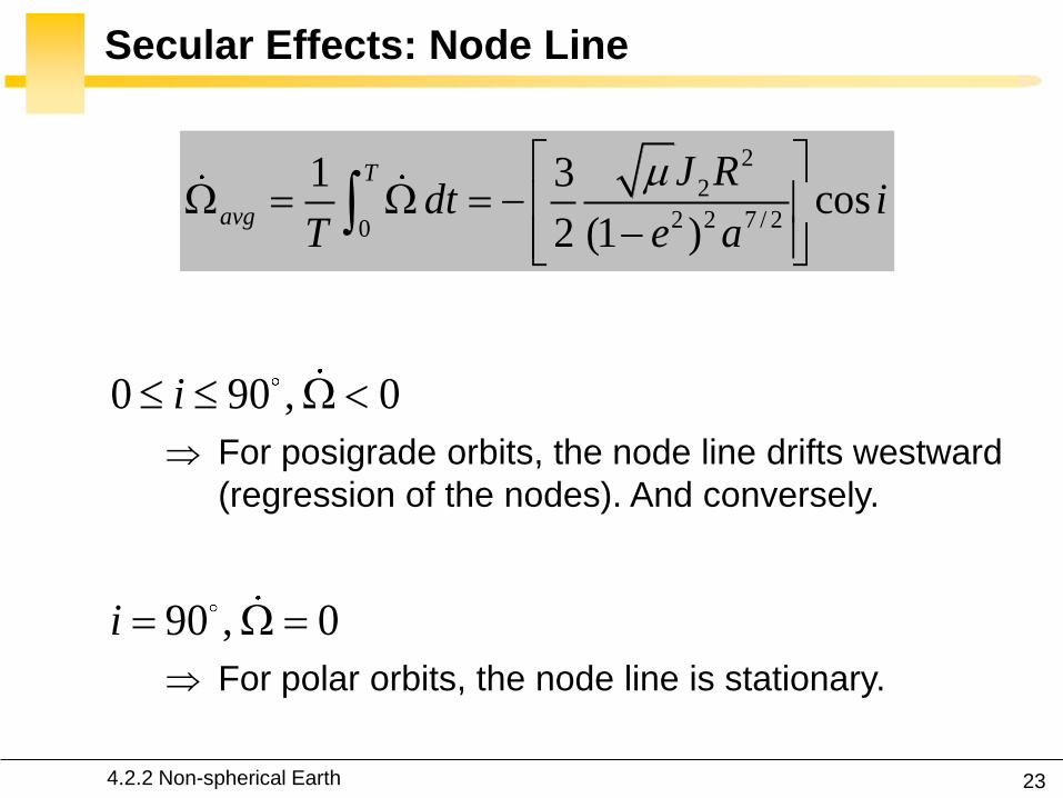
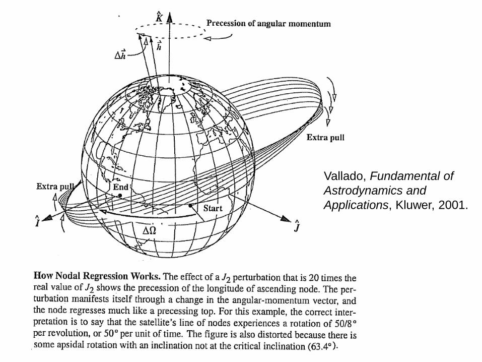
Vallado Fundamental of
Astrodynamics and
Applications Kluwer 2001
25
Exploitation Sun-Synchronous Orbits
The orbital plane makes a constant angle with the radial
from the sun
422 Non-spherical Earth
26
Exploitation Sun-Synchronous Orbits
The orbital plane must rotate in inertial space with the
angular velocity of the Earth in its orbit around the Sun
360ordm per 36526 days or 09856ordm per day
The satellite sees any given swath of the planet under
nearly the same condition of daylight or darkness day after
day
422 Non-spherical Earth
27
Existing Satellites
SPOT-5
(820 kms 987ordm)
NOAAPOES
(833 kms 987ordm)
28
Secular Effects Apse Line
2
22
2 2 7 20
1 34 5sin
4 (1 )
T
avg
J Rdt i
T e a
The perigee advances in the direction of the motion
of the satellite And conversely
0 634 or 1166 180 0i i
The apse line does not move
634 or 1166 0i i
422 Non-spherical Earth
Vallado Fundamental of
Astrodynamics and
Applications Kluwer 2001
30
Exploitation Molniya Orbits
A geostationary satellite cannot view effectively the far
northern latitudes into which Russian territory extends
(+ costly plane change maneuver for the launch vehicle )
Molniya telecommunications satellites are launched from
Plesetsk (628ordmN) into 63ordm inclination orbits having a
period of 12 hours
3
2 the apse line is 53000km longellip
aT
422 Non-spherical Earth
31
Analytic Propagators in STK 2-body J2
2-body constant orbital elements
J2 accounts for secular variations in the orbit elements
due to Earth oblateness periodic variations are
neglected
423 J2 propagator in STK
32
J2 Propagator Underlying Equations
423 J2 propagator in STK
33
2-body and J2 Propagators Applied to ISS
Two-body propagator J2 propagator
423 J2 propagator in STK
34
HPOP and J2 Propagators Applied to ISS
Nodal regression of the ISS
35
Effects of Atmospheric Drag Semi-Major Axis
2a
Lecture 2
2
2
2
2
aa
gt0
Because drag causes the dissipation of mechanical energy
from the system the semimajor axis contracts
424 Atmospheric drag
Drag paradox the effect of atmospheric drag is to increase
the satellite speed and kinetic energy
36
Effects of Atmospheric Drag Semi-Major Axis
21 10
2 2D r D
A AN R T C v C
m m a
0D
Aa a C
m
2
Df i f i
C Aa a t t
m
is assumed constant
424 Atmospheric drag
3
22 Resin 1 cos
1
aa T e
e
Circular orbit
37
Effects of Atmospheric Drag Orbit Plane
2
2sin(1 )
sin 1 cos
Na e
i e
2
2cos(1 )
1 cos
Na ei
e
The orientation of the orbit plane is not changed by drag
424 Atmospheric drag
38
Effects of Atmospheric Drag Apogee Perigee
Apogee height changes drastically perigee height remains
relatively constant
424 Atmospheric drag
Vallado Fundamental of Astrodynamics and Applications Kluwer 2001
39
Effects of Atmospheric Drag Eccentricity
Vallado Fundamental of Astrodynamics and Applications Kluwer 2001
424 Atmospheric drag
40
Early Reentry of Skylab (1979)
Increased solar activity which
increased drag on Skylab led to
an early reentry
Earth reentry footprint could not
be accurately predicted (due to
tumbling and other parameters)
Debris was found around
Esperance (31ndash34degS 122ndash
126degE) The Shire of Esperance
fined the United States $400 for
littering a fine which to this day
remains unpaid
424 Atmospheric drag
41
Lost of ASCA Satellite (2000)
July 15 2000 a strong solar
flare heated the Earthrsquos
atmosphere increasing the
air density to a value 100
times greater than that for
which its ADCS had been
designed to cope The
magnetorquers were unable
to compensate and the
satellite was lost
httpheasarcgsfcnasagovdocsascasafemodehtml
424 Atmospheric drag
42
Effects of Third-Body Perturbations
The only secular perturbations are in the node and in the
perigee
For near-Earth orbits the dominance of the oblateness
dictates that the orbital plane regresses about the polar
axis For higher orbits the regression will be about some
mean pole lying between the Earthrsquos pole and the ecliptic
pole
Many geosynchronous satellites launched 30 years ago
now have inclinations of up to plusmn15ordm collision avoidance
as the satellites drift back through the GEO belt
425 Third-body perturbations
43
Effects of Third-Body Perturbations
Vallado Fundamental of Astrodynamics and Applications Kluwer 2001
The Sunrsquos attraction
tends to turn the
satellite ring into the
ecliptic The orbit
precesses about the
pole of the ecliptic
425 Third-body perturbations
44
STK Analytic Propagator (SGP4)
The J2 propagator does not include drag
SGP4 which stands for Simplified General Perturbations
Satellite Orbit Model 4 is a NASANORAD algorithm
426 SGP4 propagator in STK
45
STK Analytic Propagator (SGP4)
Several assumptions propagation valid for short durations
(3-10 days)
TLE data should be used as the input (see Lecture 03)
It considers secular and periodic variations due to Earth
oblateness solar and lunar gravitational effects and
orbital decay using a drag model
426 SGP4 propagator in STK
46
SGP4 Applied to ISS RAAN
426 SGP4 propagator in STK
47
SGP4 Applied to ISS Semi-Major Axis
426 SGP4 propagator in STK
48
Further Reading on the Web Site
426 SGP4 propagator in STK
49
Effects of Solar Radiation Pressure
The effects are usually small for most satellites
Satellites with very low mass and large surface area are
more affected
427 Solar radiation pressure
Vallado Fundamental of
Astrodynamics and
Applications Kluwer
2001
51
Secular Effects Orders of Magnitude
Vallado Fundamental of Astrodynamics and Applications Kluwer 2001
52
Periodic Effects Orders of Magnitude
Vallado Fundamental of Astrodynamics and Applications Kluwer 2001
53
4 Non-Keplerian Motion
2
2
(1 )
sin
sin 1 cos
a e
N
i e
43 Numerical methods
431 Orbit prediction
432 Numerical integration
433 Single-step methods Runge-Kutta
434 Multi-step methods
435 Integrator and step size selection
436 ISS example
nt 1nt
r
54
2-body analytic propagator (constant orbital elements)
J2 analytic propagator (secular variations in the orbit
elements due to Earth oblateness
HPOP numerical integration of the equations of motion
(periodic and secular effects included)
STK Propagators
431 Orbit prediction
Accurate
Versatile
Errors accumulation
for long intervals
Computationally
intensive
55
Real-Life Example German Aerospace Agency
431 Orbit prediction
56
Real-Life Example German Aerospace Agency
57
Further Reading on the Web Site
431 Orbit prediction
58
Real-Life Example Envisat
httpnngesocesadeenvisat
ENVpredhtml
431 Orbit prediction
Why do the
predictions degrade
for lower altitudes
60
NASA began the first complex numerical integrations
during the late 1960s and early 1970s
Did you Know
1969 1968
431 Orbit prediction
61
What is Numerical Integration
1n nt t t
3 perturbedr
r r a
Given
Compute
( ) ( )n nt tr r
1 1( ) ( )n nt t r r
432 Numerical integration
62
State-Space Formulation
3 perturbedr
r r a
( )f tu u
ru
r
6-dimensional
state vector
432 Numerical integration
63
How to Perform Numerical Integration
2( )( ) ( ) ( ) ( ) ( )
2
ss
n n n n n s
h hf t h f t hf t f t f t R
s
Taylor series expansion
( )ntu
1( )nt u
432 Numerical integration
64
First-Order Taylor Approximation (Euler)
1
( ) ( ) ( )
( )
n n n
n n n n
t t t t t
t f t
u u u
u u uEuler step
0 1 2 3 4 5 60
5
10
15
20
25
30
35
40
Time t (s)
x(t
)=t2
Exact solution
The stepsize has to be extremely
small for accurate predictions
and it is necessary to develop
more effective algorithms
along the tangent
432 Numerical integration
65
Numerical Integration Methods
1 1 1
1 0
m m
n j n j j n j
j j
t
u u u
0 0
Implicit the solution method becomes
iterative in the nonlinear case
0 0 Explicit un+1 can be deduced directly from
the results at the previous time steps
=0
for 1
j j
j
Single-step the system at time tn+1
only depends on the previous state tn
State vector
0
for 1
j j
j
Multi-step the system at time tn+1 depends
several previous states tntn-1etc
432 Numerical integration
66
Examples Implicit vs Explicit
Trapezoidal rule (implicit)
nt 1nt
Euler forward (explicit)
nt 1nt
Euler backward (implicit)
nt 1nt
1n n nt u u u
1 1n n nt u u u
1
12
n n
n n t
u uu u
r
r
r
432 Numerical integration
67
A variety of methods has been applied in astrodynamics
Each of these methods has its own advantages and
drawbacks
Accuracy what is the order of the integration scheme
Efficiency how many function calls
Versatility can it be applied to a wide range of problems
Complexity is it easy to implement and use
Step size automatic step size control
Why Different Methods
431 Orbit prediction
68
Runge-Kutta Family Single-Step
Perhaps the most well-known numerical integrator
Difference with traditional Taylor series integrators the RK
family only requires the first derivative but several
evaluations are needed to move forward one step in time
Different variants explicit embedded etc
433 Single-step methods Runge-Kutta
69
Runge-Kutta Family Single-Step
with ( ) ( )t f tu u 0 0( )t u u
1
1
s
n n i i
i
t b
u u k
1 1
1
1
2
n n
i
i n ij j n i
j
f t c t
f t a t c t i s
k u
k u k
Slopes at
various points
within the
integration step
433 Single-step methods Runge-Kutta
70
Runge-Kutta Family Single-Step
Butcher Tableau
The Runge-Kutta methods are fully described by the
coefficients
c1
c2
cs
a21
as1
b1
as2
b2
ass-1
bs-1 hellip
hellip
hellip hellip hellip
bs
1
1
1
1
1
0
s
i
i
i
i ij
j
b
c
c a
433 Single-step methods Runge-Kutta
71
RK4 (Explicit)
1 2 3 41
2 2
6n n t
k k k ku u
Butcher Tableau
1
2 1
3 2
4 3
2 2
2 2
n n
n n
n n
n n
f t
t tf t
t tf t
f t t t
k u
k u k
k u k
k u k
433 Single-step methods Runge-Kutta
72
RK4 (Explicit)
1 2 3 41
2 2
6n n t
k k k ku u
1
2 1
3 2
4 3
2 2
2 2
n n
n n
n n
n n
f t
t tf t
t tf t
f t t t
k u
k u k
k u k
k u k
Slope at the beginning
Slope at the midpoint (k1 is
used to determine the value
of u Euler)
Slope at the midpoint (k2 is
now used)
Slope at the end
Estimated slope
(weighted average)
433 Single-step methods Runge-Kutta
73
RK4 (Explicit)
nt 2nt t nt t
1k3k
2k
4k
Estimate at new
time
u
433 Single-step methods Runge-Kutta
74
RK4 (Explicit)
The local truncation error for a 4th order RK is O(h5)
The accuracy is comparable to that of a 4th order Taylor
series but the Runge-Kutta method avoids the
calculation of higher-order derivatives
Easy to use and implement
The step size is fixed
433 Single-step methods Runge-Kutta
75
RK4 in STK
433 Single-step methods Runge-Kutta
76
Embedded Methods
They produce an estimate of the local truncation error
adjust the step size to keep local truncation errors
within some tolerances
This is done by having two methods in the tableau one with
order p and one with order p+1 with the same set of
function evaluations
( 1) ( 1) ( 1)
1
1
sp p p
n n i i
i
t b
u u k
( ) ( ) ( )
1
1
sp p p
n n i i
i
t b
u u k
433 Single-step methods Runge-Kutta
77
Embedded Methods
The two different approximations for the solution at each
step are compared
If the two answers are in close agreement the approximation is
accepted
If the two answers do not agree to a specified accuracy the step
size is reduced
If the answers agree to more significant digits than required the
step size is increased
433 Single-step methods Runge-Kutta
78
Ode45 in Matlab Simulink
Runge-Kutta (45) pair of Dormand and Prince
Variable step size
Matlab help This should be the first solver you try
433 Single-step methods Runge-Kutta
79
Ode45 in Matlab Simulink
edit ode45
433 Single-step methods Runge-Kutta
80
Ode45 in Matlab Simulink
Be very careful with the default parameters
options = odeset(RelTol1e-8AbsTol1e-8)
433 Single-step methods Runge-Kutta
81
RKF 7(8) Default Method in STK
Runge-Kutta-Fehlberg integration method of 7th order
with 8th order error control for the integration step size
433 Single-step methods Runge-Kutta
83
Multi-Step Methods (Predictor-Corrector)
They estimate the state over time using previously
determined back values of the solution
Unlike RK methods they only perform one evaluation for
each step forward but they usually have a predictor and a
corrector formula
Adams() ndash Bashforth - Moulton Gauss - Jackson
() The first with Le Verrier to predict the existence and position of Neptune
434 Multi-step methods
84
Multi-Step Methods Principle
( ) ( )t f tu u1
1( ) ( ) ( ) n
n
t
n nt
t t f t dt
u u u
unknown
Replace it by a
polynomial that
interpolates the
previous values Four function values
interpolated by a
third-order polynomial
t
u
434 Multi-step methods
85
Multi-Step Methods Initiation
with ( ) ( )t f tu u 0 0( )t u u
What is the inherent problem
t
u
434 Multi-step methods
86
Multi-Step Methods Initiation
Because these methods require back values they are not
self-starting
One may for instance use of a single-step method to
compute the first four values
434 Multi-step methods
87
Gauss-Jackson in STK
One of the most recommendable fixed-stepsize multistep
methods for orbit computations
88
Integrator Selection
435 Integrator and step size selection
Montenbruck and Gill
Satellite orbits Springer
2000
89
Integrator Selection
Pros
Very fast
Cons
Special starting procedure
Fixed time steps
Error control
Pros
Plug and play
Error control
Cons
Slower
Multi-step Single step
435 Integrator and step size selection
90
Why is the Step Size So Critical
Theoretical arguments
1 The accuracy and the stability of the algorithm are
directly related to the step size
2 Nonlinear equations of motion
Data for Landsat 4 and 6 in circular orbits around 800km
indicates that a one-minute step size yields about 47m
error
A three-minute step size produces about a 900m error
435 Integrator and step size selection
91
Why is the Step Size So Critical
More practical arguments
1 The computation time is directly related to the
step size
2 The particular choice of step size depends on the
most rapidly varying component in the disturbing
functions (eg 50 x 50 gravity field)
435 Integrator and step size selection
92
Appropriate Step Size
The problem of determining an appropriate step size is a
challenge in any numerical process
Fixed step size (rule of thumb for standard
applications)
But an algorithm with variable step size is really
helpful The step size is chosen in such a way that
each step contributes uniformly to the total integration
error
100
orbitTt
435 Integrator and step size selection
93
Three Examples XMM OUFTI-1 ISS
Can you plot the step size vs true anomaly
435 Integrator and step size selection
94
XMM Report in STK
435 Integrator and step size selection
95
XMM (e~08)
0 50 100 150 200 250 300 350 4000
1000
2000
3000
4000
5000
6000
True anomaly (deg)
Ste
p s
ize
(s)
435 Integrator and step size selection
96
ISS(e~0)
435 Integrator and step size selection
0 50 100 150 200 250 300 350 40030
35
40
45
50
55
60
65
70
True anomaly (deg)
Ste
p s
ize
(s)
97
ldquoDifficultrdquo Orbits
Automatic time step is especially nice on highly eccentric
orbits (Molniya XMM) These orbits are best computed
using variable step sizes to maintain some given level of
accuracy
Without this variable step size we waste a lot of time near
apoapsis when the integration is taking too small a step
Likewise the integrator may not be using a small enough step
size at periapsis where the satellite is traveling fast
435 Integrator and step size selection
98
HPOP Propagator ISS Example
1 Earthrsquos oblateness only
2 Drag only
3 Sun and moon only
4 SRP only
5 All together
436 ISS example
99
Earthrsquos Oblateness Only Ω
HPOP
J2
2-body
436 ISS example
100
Earthrsquos Oblateness Only i Ω a
HPOP with central body (20 + WGS84_EGM96)
(without dragSRPSun and Moon)
436 ISS example
101
Drag Only i Ω a
HPOP with drag ndash Harris Priester
(without oblatenessSRPSun and Moon)
436 ISS example
102
Drag Relationship with Eclipses
103
SRP Only i Ω a
HPOP with SRP
(without oblatenessdragSun and Moon)
436 ISS example
104
SRP Relationship with Eclipses
105
All Perturbations Together
436 ISS example
106
4 Non-Keplerian Motion
2
2
(1 )
sin
sin 1 cos
a e
N
i e
44 Geostationary satellites
107
Practical Example GEO Satellites
Nice illustration of
1 Perturbations of the 2-body problem
2 Secular and periodic contributions
3 Accuracy required by practical applications
4 The need for orbit correction and thrust forces
And it is a real-life example (telecommunications
meteorology)
44 GEO satellites
108
Three Main Perturbations for GEO Satellites
44 GEO satellites
1 Non-spherical Earth
2 SRP
3 Sun and Moon
109
Station Keeping of GEO Satellites
The effect of the perturbations is to cause the spacecraft
to drift away from its nominal station If the drift was
allowed to build up unchecked the spacecraft could
become useless
A station-keeping box is defined by a longitude and a
maximum authorized distance for satellite excursions in
longitude and latitude
For instance TC2 -8ordm plusmn 007ordm EW plusmn 005ordm NS
44 GEO satellites
110
East-West and North-South Drift
44 GEO satellites
NS drift
EW drift
What are the perturbations generating these drifts
111
East-West Drift
44 GEO satellites
A GEO satellite drifts in longitude due to the influence of
two main perturbations
1 The elliptic nature of the Earthrsquos equatorial cross-
section J22 (and not from the NS oblateness J2)
2
ΔV
ΔV vsat
vsat SRP
112
East-West Drift due to Equatorial Ellipticity
44 GEO satellites
113
East-West Drift due to Equatorial Ellipticity
44 GEO satellites
114
East-West Drift HPOP (20) vs HPOP (22)
44 GEO satellites
115
East-West Drift Stable Equilibirum
HPOP with 22
(without Sun and moonSRPdrag)
116
East-West Drift Stable Equilibirum
HPOP with 22
(without Sun and moonSRPdrag)
117
East-West Drift Stable Equilibirum
HPOP with 22
(without Sun and moonSRPdrag)
118
North-South Drift
The perturbations caused by the Sun and the Moon are
predominantly out-of-plane effects causing a change in
the inclination and in the right ascension of the orbit
ascending node
Similar effects on the orbit to those of the Earthrsquos
oblateness (but here with respect to the ecliptic)
A GEO satellite therefore drifts in latitude with a
fundamental period equal to the orbit period
119
North-South Drift
Period
HPOP with Sun and Moon
(without oblatenessSRPdrag)
120
North-South Drift
Period
HPOP with Sun and Moon
(without oblatenessSRPdrag)
121
Thrust Forces for Stationkeeping
GEO spacecraft require continual stationkeeping to stay
within the authorized box using onboard thrusters
44 GEO satellites
122
42 ANALYTIC TREATMENT
421 Variation of parameters
422 Non-spherical Earth
423 J2 propagator in STK
424 Atmospheric drag
425 Third-body perturbations
426 SGP4 propagator in STK
427 Solar radiation pressure
4 Non-Keplerian Motion
43 NUMERICAL METHODS
431 Orbit prediction
432 Numerical integration
433 Single-step methods Runge-Kutta
434 Multi-step methods
435 Integrator and step size selection
436 ISS example
44 GEOSTATIONARY SATELLITES
Gaeumltan Kerschen
Space Structures amp
Systems Lab (S3L)
4B Non-Keplerian Motion
Astrodynamics (AERO0024)
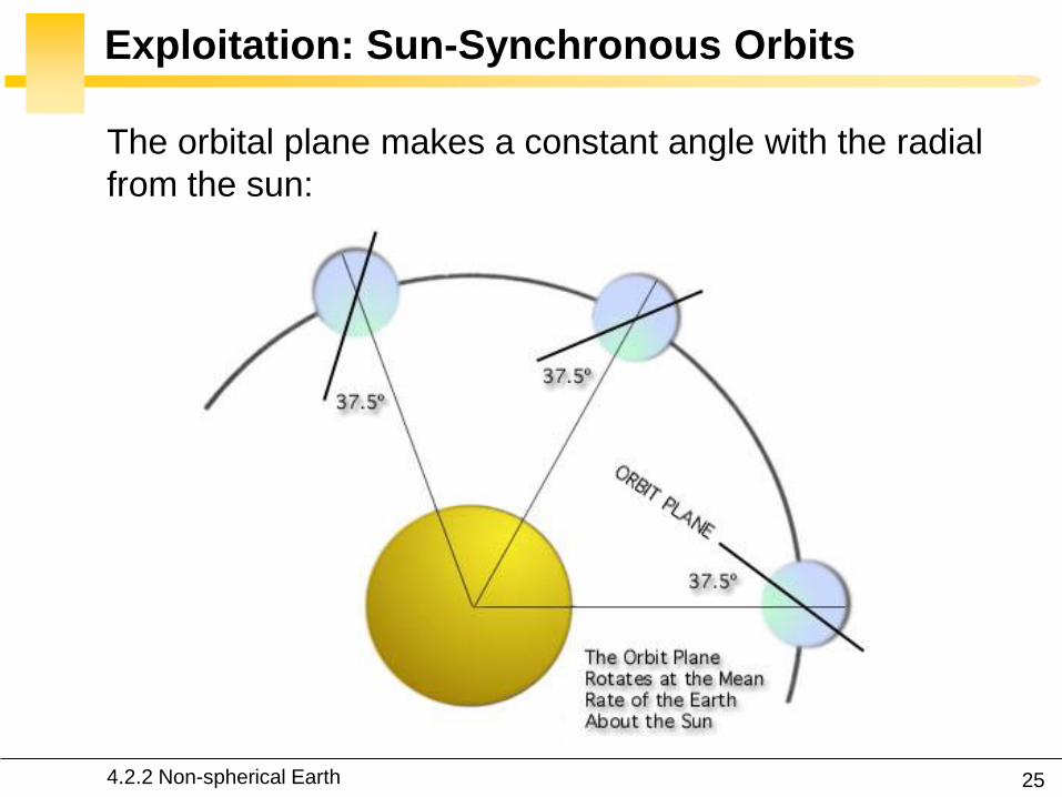
25
Exploitation Sun-Synchronous Orbits
The orbital plane makes a constant angle with the radial
from the sun
422 Non-spherical Earth
26
Exploitation Sun-Synchronous Orbits
The orbital plane must rotate in inertial space with the
angular velocity of the Earth in its orbit around the Sun
360ordm per 36526 days or 09856ordm per day
The satellite sees any given swath of the planet under
nearly the same condition of daylight or darkness day after
day
422 Non-spherical Earth
27
Existing Satellites
SPOT-5
(820 kms 987ordm)
NOAAPOES
(833 kms 987ordm)
28
Secular Effects Apse Line
2
22
2 2 7 20
1 34 5sin
4 (1 )
T
avg
J Rdt i
T e a
The perigee advances in the direction of the motion
of the satellite And conversely
0 634 or 1166 180 0i i
The apse line does not move
634 or 1166 0i i
422 Non-spherical Earth
Vallado Fundamental of
Astrodynamics and
Applications Kluwer 2001
30
Exploitation Molniya Orbits
A geostationary satellite cannot view effectively the far
northern latitudes into which Russian territory extends
(+ costly plane change maneuver for the launch vehicle )
Molniya telecommunications satellites are launched from
Plesetsk (628ordmN) into 63ordm inclination orbits having a
period of 12 hours
3
2 the apse line is 53000km longellip
aT
422 Non-spherical Earth
31
Analytic Propagators in STK 2-body J2
2-body constant orbital elements
J2 accounts for secular variations in the orbit elements
due to Earth oblateness periodic variations are
neglected
423 J2 propagator in STK
32
J2 Propagator Underlying Equations
423 J2 propagator in STK
33
2-body and J2 Propagators Applied to ISS
Two-body propagator J2 propagator
423 J2 propagator in STK
34
HPOP and J2 Propagators Applied to ISS
Nodal regression of the ISS
35
Effects of Atmospheric Drag Semi-Major Axis
2a
Lecture 2
2
2
2
2
aa
gt0
Because drag causes the dissipation of mechanical energy
from the system the semimajor axis contracts
424 Atmospheric drag
Drag paradox the effect of atmospheric drag is to increase
the satellite speed and kinetic energy
36
Effects of Atmospheric Drag Semi-Major Axis
21 10
2 2D r D
A AN R T C v C
m m a
0D
Aa a C
m
2
Df i f i
C Aa a t t
m
is assumed constant
424 Atmospheric drag
3
22 Resin 1 cos
1
aa T e
e
Circular orbit
37
Effects of Atmospheric Drag Orbit Plane
2
2sin(1 )
sin 1 cos
Na e
i e
2
2cos(1 )
1 cos
Na ei
e
The orientation of the orbit plane is not changed by drag
424 Atmospheric drag
38
Effects of Atmospheric Drag Apogee Perigee
Apogee height changes drastically perigee height remains
relatively constant
424 Atmospheric drag
Vallado Fundamental of Astrodynamics and Applications Kluwer 2001
39
Effects of Atmospheric Drag Eccentricity
Vallado Fundamental of Astrodynamics and Applications Kluwer 2001
424 Atmospheric drag
40
Early Reentry of Skylab (1979)
Increased solar activity which
increased drag on Skylab led to
an early reentry
Earth reentry footprint could not
be accurately predicted (due to
tumbling and other parameters)
Debris was found around
Esperance (31ndash34degS 122ndash
126degE) The Shire of Esperance
fined the United States $400 for
littering a fine which to this day
remains unpaid
424 Atmospheric drag
41
Lost of ASCA Satellite (2000)
July 15 2000 a strong solar
flare heated the Earthrsquos
atmosphere increasing the
air density to a value 100
times greater than that for
which its ADCS had been
designed to cope The
magnetorquers were unable
to compensate and the
satellite was lost
httpheasarcgsfcnasagovdocsascasafemodehtml
424 Atmospheric drag
42
Effects of Third-Body Perturbations
The only secular perturbations are in the node and in the
perigee
For near-Earth orbits the dominance of the oblateness
dictates that the orbital plane regresses about the polar
axis For higher orbits the regression will be about some
mean pole lying between the Earthrsquos pole and the ecliptic
pole
Many geosynchronous satellites launched 30 years ago
now have inclinations of up to plusmn15ordm collision avoidance
as the satellites drift back through the GEO belt
425 Third-body perturbations
43
Effects of Third-Body Perturbations
Vallado Fundamental of Astrodynamics and Applications Kluwer 2001
The Sunrsquos attraction
tends to turn the
satellite ring into the
ecliptic The orbit
precesses about the
pole of the ecliptic
425 Third-body perturbations
44
STK Analytic Propagator (SGP4)
The J2 propagator does not include drag
SGP4 which stands for Simplified General Perturbations
Satellite Orbit Model 4 is a NASANORAD algorithm
426 SGP4 propagator in STK
45
STK Analytic Propagator (SGP4)
Several assumptions propagation valid for short durations
(3-10 days)
TLE data should be used as the input (see Lecture 03)
It considers secular and periodic variations due to Earth
oblateness solar and lunar gravitational effects and
orbital decay using a drag model
426 SGP4 propagator in STK
46
SGP4 Applied to ISS RAAN
426 SGP4 propagator in STK
47
SGP4 Applied to ISS Semi-Major Axis
426 SGP4 propagator in STK
48
Further Reading on the Web Site
426 SGP4 propagator in STK
49
Effects of Solar Radiation Pressure
The effects are usually small for most satellites
Satellites with very low mass and large surface area are
more affected
427 Solar radiation pressure
Vallado Fundamental of
Astrodynamics and
Applications Kluwer
2001
51
Secular Effects Orders of Magnitude
Vallado Fundamental of Astrodynamics and Applications Kluwer 2001
52
Periodic Effects Orders of Magnitude
Vallado Fundamental of Astrodynamics and Applications Kluwer 2001
53
4 Non-Keplerian Motion
2
2
(1 )
sin
sin 1 cos
a e
N
i e
43 Numerical methods
431 Orbit prediction
432 Numerical integration
433 Single-step methods Runge-Kutta
434 Multi-step methods
435 Integrator and step size selection
436 ISS example
nt 1nt
r
54
2-body analytic propagator (constant orbital elements)
J2 analytic propagator (secular variations in the orbit
elements due to Earth oblateness
HPOP numerical integration of the equations of motion
(periodic and secular effects included)
STK Propagators
431 Orbit prediction
Accurate
Versatile
Errors accumulation
for long intervals
Computationally
intensive
55
Real-Life Example German Aerospace Agency
431 Orbit prediction
56
Real-Life Example German Aerospace Agency
57
Further Reading on the Web Site
431 Orbit prediction
58
Real-Life Example Envisat
httpnngesocesadeenvisat
ENVpredhtml
431 Orbit prediction
Why do the
predictions degrade
for lower altitudes
60
NASA began the first complex numerical integrations
during the late 1960s and early 1970s
Did you Know
1969 1968
431 Orbit prediction
61
What is Numerical Integration
1n nt t t
3 perturbedr
r r a
Given
Compute
( ) ( )n nt tr r
1 1( ) ( )n nt t r r
432 Numerical integration
62
State-Space Formulation
3 perturbedr
r r a
( )f tu u
ru
r
6-dimensional
state vector
432 Numerical integration
63
How to Perform Numerical Integration
2( )( ) ( ) ( ) ( ) ( )
2
ss
n n n n n s
h hf t h f t hf t f t f t R
s
Taylor series expansion
( )ntu
1( )nt u
432 Numerical integration
64
First-Order Taylor Approximation (Euler)
1
( ) ( ) ( )
( )
n n n
n n n n
t t t t t
t f t
u u u
u u uEuler step
0 1 2 3 4 5 60
5
10
15
20
25
30
35
40
Time t (s)
x(t
)=t2
Exact solution
The stepsize has to be extremely
small for accurate predictions
and it is necessary to develop
more effective algorithms
along the tangent
432 Numerical integration
65
Numerical Integration Methods
1 1 1
1 0
m m
n j n j j n j
j j
t
u u u
0 0
Implicit the solution method becomes
iterative in the nonlinear case
0 0 Explicit un+1 can be deduced directly from
the results at the previous time steps
=0
for 1
j j
j
Single-step the system at time tn+1
only depends on the previous state tn
State vector
0
for 1
j j
j
Multi-step the system at time tn+1 depends
several previous states tntn-1etc
432 Numerical integration
66
Examples Implicit vs Explicit
Trapezoidal rule (implicit)
nt 1nt
Euler forward (explicit)
nt 1nt
Euler backward (implicit)
nt 1nt
1n n nt u u u
1 1n n nt u u u
1
12
n n
n n t
u uu u
r
r
r
432 Numerical integration
67
A variety of methods has been applied in astrodynamics
Each of these methods has its own advantages and
drawbacks
Accuracy what is the order of the integration scheme
Efficiency how many function calls
Versatility can it be applied to a wide range of problems
Complexity is it easy to implement and use
Step size automatic step size control
Why Different Methods
431 Orbit prediction
68
Runge-Kutta Family Single-Step
Perhaps the most well-known numerical integrator
Difference with traditional Taylor series integrators the RK
family only requires the first derivative but several
evaluations are needed to move forward one step in time
Different variants explicit embedded etc
433 Single-step methods Runge-Kutta
69
Runge-Kutta Family Single-Step
with ( ) ( )t f tu u 0 0( )t u u
1
1
s
n n i i
i
t b
u u k
1 1
1
1
2
n n
i
i n ij j n i
j
f t c t
f t a t c t i s
k u
k u k
Slopes at
various points
within the
integration step
433 Single-step methods Runge-Kutta
70
Runge-Kutta Family Single-Step
Butcher Tableau
The Runge-Kutta methods are fully described by the
coefficients
c1
c2
cs
a21
as1
b1
as2
b2
ass-1
bs-1 hellip
hellip
hellip hellip hellip
bs
1
1
1
1
1
0
s
i
i
i
i ij
j
b
c
c a
433 Single-step methods Runge-Kutta
71
RK4 (Explicit)
1 2 3 41
2 2
6n n t
k k k ku u
Butcher Tableau
1
2 1
3 2
4 3
2 2
2 2
n n
n n
n n
n n
f t
t tf t
t tf t
f t t t
k u
k u k
k u k
k u k
433 Single-step methods Runge-Kutta
72
RK4 (Explicit)
1 2 3 41
2 2
6n n t
k k k ku u
1
2 1
3 2
4 3
2 2
2 2
n n
n n
n n
n n
f t
t tf t
t tf t
f t t t
k u
k u k
k u k
k u k
Slope at the beginning
Slope at the midpoint (k1 is
used to determine the value
of u Euler)
Slope at the midpoint (k2 is
now used)
Slope at the end
Estimated slope
(weighted average)
433 Single-step methods Runge-Kutta
73
RK4 (Explicit)
nt 2nt t nt t
1k3k
2k
4k
Estimate at new
time
u
433 Single-step methods Runge-Kutta
74
RK4 (Explicit)
The local truncation error for a 4th order RK is O(h5)
The accuracy is comparable to that of a 4th order Taylor
series but the Runge-Kutta method avoids the
calculation of higher-order derivatives
Easy to use and implement
The step size is fixed
433 Single-step methods Runge-Kutta
75
RK4 in STK
433 Single-step methods Runge-Kutta
76
Embedded Methods
They produce an estimate of the local truncation error
adjust the step size to keep local truncation errors
within some tolerances
This is done by having two methods in the tableau one with
order p and one with order p+1 with the same set of
function evaluations
( 1) ( 1) ( 1)
1
1
sp p p
n n i i
i
t b
u u k
( ) ( ) ( )
1
1
sp p p
n n i i
i
t b
u u k
433 Single-step methods Runge-Kutta
77
Embedded Methods
The two different approximations for the solution at each
step are compared
If the two answers are in close agreement the approximation is
accepted
If the two answers do not agree to a specified accuracy the step
size is reduced
If the answers agree to more significant digits than required the
step size is increased
433 Single-step methods Runge-Kutta
78
Ode45 in Matlab Simulink
Runge-Kutta (45) pair of Dormand and Prince
Variable step size
Matlab help This should be the first solver you try
433 Single-step methods Runge-Kutta
79
Ode45 in Matlab Simulink
edit ode45
433 Single-step methods Runge-Kutta
80
Ode45 in Matlab Simulink
Be very careful with the default parameters
options = odeset(RelTol1e-8AbsTol1e-8)
433 Single-step methods Runge-Kutta
81
RKF 7(8) Default Method in STK
Runge-Kutta-Fehlberg integration method of 7th order
with 8th order error control for the integration step size
433 Single-step methods Runge-Kutta
83
Multi-Step Methods (Predictor-Corrector)
They estimate the state over time using previously
determined back values of the solution
Unlike RK methods they only perform one evaluation for
each step forward but they usually have a predictor and a
corrector formula
Adams() ndash Bashforth - Moulton Gauss - Jackson
() The first with Le Verrier to predict the existence and position of Neptune
434 Multi-step methods
84
Multi-Step Methods Principle
( ) ( )t f tu u1
1( ) ( ) ( ) n
n
t
n nt
t t f t dt
u u u
unknown
Replace it by a
polynomial that
interpolates the
previous values Four function values
interpolated by a
third-order polynomial
t
u
434 Multi-step methods
85
Multi-Step Methods Initiation
with ( ) ( )t f tu u 0 0( )t u u
What is the inherent problem
t
u
434 Multi-step methods
86
Multi-Step Methods Initiation
Because these methods require back values they are not
self-starting
One may for instance use of a single-step method to
compute the first four values
434 Multi-step methods
87
Gauss-Jackson in STK
One of the most recommendable fixed-stepsize multistep
methods for orbit computations
88
Integrator Selection
435 Integrator and step size selection
Montenbruck and Gill
Satellite orbits Springer
2000
89
Integrator Selection
Pros
Very fast
Cons
Special starting procedure
Fixed time steps
Error control
Pros
Plug and play
Error control
Cons
Slower
Multi-step Single step
435 Integrator and step size selection
90
Why is the Step Size So Critical
Theoretical arguments
1 The accuracy and the stability of the algorithm are
directly related to the step size
2 Nonlinear equations of motion
Data for Landsat 4 and 6 in circular orbits around 800km
indicates that a one-minute step size yields about 47m
error
A three-minute step size produces about a 900m error
435 Integrator and step size selection
91
Why is the Step Size So Critical
More practical arguments
1 The computation time is directly related to the
step size
2 The particular choice of step size depends on the
most rapidly varying component in the disturbing
functions (eg 50 x 50 gravity field)
435 Integrator and step size selection
92
Appropriate Step Size
The problem of determining an appropriate step size is a
challenge in any numerical process
Fixed step size (rule of thumb for standard
applications)
But an algorithm with variable step size is really
helpful The step size is chosen in such a way that
each step contributes uniformly to the total integration
error
100
orbitTt
435 Integrator and step size selection
93
Three Examples XMM OUFTI-1 ISS
Can you plot the step size vs true anomaly
435 Integrator and step size selection
94
XMM Report in STK
435 Integrator and step size selection
95
XMM (e~08)
0 50 100 150 200 250 300 350 4000
1000
2000
3000
4000
5000
6000
True anomaly (deg)
Ste
p s
ize
(s)
435 Integrator and step size selection
96
ISS(e~0)
435 Integrator and step size selection
0 50 100 150 200 250 300 350 40030
35
40
45
50
55
60
65
70
True anomaly (deg)
Ste
p s
ize
(s)
97
ldquoDifficultrdquo Orbits
Automatic time step is especially nice on highly eccentric
orbits (Molniya XMM) These orbits are best computed
using variable step sizes to maintain some given level of
accuracy
Without this variable step size we waste a lot of time near
apoapsis when the integration is taking too small a step
Likewise the integrator may not be using a small enough step
size at periapsis where the satellite is traveling fast
435 Integrator and step size selection
98
HPOP Propagator ISS Example
1 Earthrsquos oblateness only
2 Drag only
3 Sun and moon only
4 SRP only
5 All together
436 ISS example
99
Earthrsquos Oblateness Only Ω
HPOP
J2
2-body
436 ISS example
100
Earthrsquos Oblateness Only i Ω a
HPOP with central body (20 + WGS84_EGM96)
(without dragSRPSun and Moon)
436 ISS example
101
Drag Only i Ω a
HPOP with drag ndash Harris Priester
(without oblatenessSRPSun and Moon)
436 ISS example
102
Drag Relationship with Eclipses
103
SRP Only i Ω a
HPOP with SRP
(without oblatenessdragSun and Moon)
436 ISS example
104
SRP Relationship with Eclipses
105
All Perturbations Together
436 ISS example
106
4 Non-Keplerian Motion
2
2
(1 )
sin
sin 1 cos
a e
N
i e
44 Geostationary satellites
107
Practical Example GEO Satellites
Nice illustration of
1 Perturbations of the 2-body problem
2 Secular and periodic contributions
3 Accuracy required by practical applications
4 The need for orbit correction and thrust forces
And it is a real-life example (telecommunications
meteorology)
44 GEO satellites
108
Three Main Perturbations for GEO Satellites
44 GEO satellites
1 Non-spherical Earth
2 SRP
3 Sun and Moon
109
Station Keeping of GEO Satellites
The effect of the perturbations is to cause the spacecraft
to drift away from its nominal station If the drift was
allowed to build up unchecked the spacecraft could
become useless
A station-keeping box is defined by a longitude and a
maximum authorized distance for satellite excursions in
longitude and latitude
For instance TC2 -8ordm plusmn 007ordm EW plusmn 005ordm NS
44 GEO satellites
110
East-West and North-South Drift
44 GEO satellites
NS drift
EW drift
What are the perturbations generating these drifts
111
East-West Drift
44 GEO satellites
A GEO satellite drifts in longitude due to the influence of
two main perturbations
1 The elliptic nature of the Earthrsquos equatorial cross-
section J22 (and not from the NS oblateness J2)
2
ΔV
ΔV vsat
vsat SRP
112
East-West Drift due to Equatorial Ellipticity
44 GEO satellites
113
East-West Drift due to Equatorial Ellipticity
44 GEO satellites
114
East-West Drift HPOP (20) vs HPOP (22)
44 GEO satellites
115
East-West Drift Stable Equilibirum
HPOP with 22
(without Sun and moonSRPdrag)
116
East-West Drift Stable Equilibirum
HPOP with 22
(without Sun and moonSRPdrag)
117
East-West Drift Stable Equilibirum
HPOP with 22
(without Sun and moonSRPdrag)
118
North-South Drift
The perturbations caused by the Sun and the Moon are
predominantly out-of-plane effects causing a change in
the inclination and in the right ascension of the orbit
ascending node
Similar effects on the orbit to those of the Earthrsquos
oblateness (but here with respect to the ecliptic)
A GEO satellite therefore drifts in latitude with a
fundamental period equal to the orbit period
119
North-South Drift
Period
HPOP with Sun and Moon
(without oblatenessSRPdrag)
120
North-South Drift
Period
HPOP with Sun and Moon
(without oblatenessSRPdrag)
121
Thrust Forces for Stationkeeping
GEO spacecraft require continual stationkeeping to stay
within the authorized box using onboard thrusters
44 GEO satellites
122
42 ANALYTIC TREATMENT
421 Variation of parameters
422 Non-spherical Earth
423 J2 propagator in STK
424 Atmospheric drag
425 Third-body perturbations
426 SGP4 propagator in STK
427 Solar radiation pressure
4 Non-Keplerian Motion
43 NUMERICAL METHODS
431 Orbit prediction
432 Numerical integration
433 Single-step methods Runge-Kutta
434 Multi-step methods
435 Integrator and step size selection
436 ISS example
44 GEOSTATIONARY SATELLITES
Gaeumltan Kerschen
Space Structures amp
Systems Lab (S3L)
4B Non-Keplerian Motion
Astrodynamics (AERO0024)
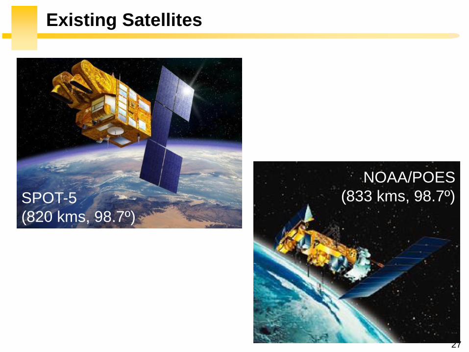
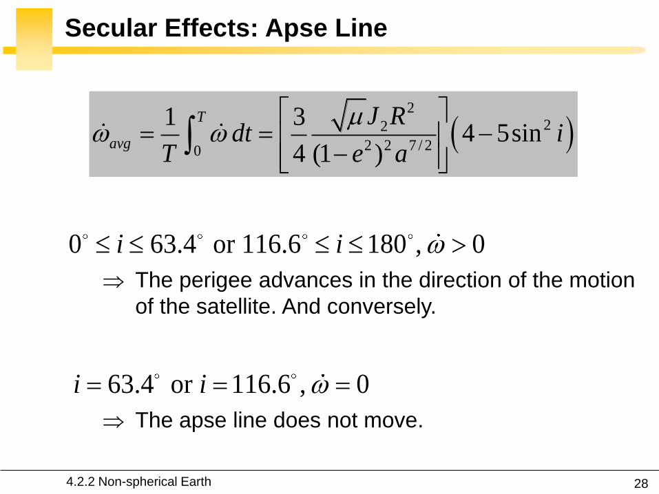
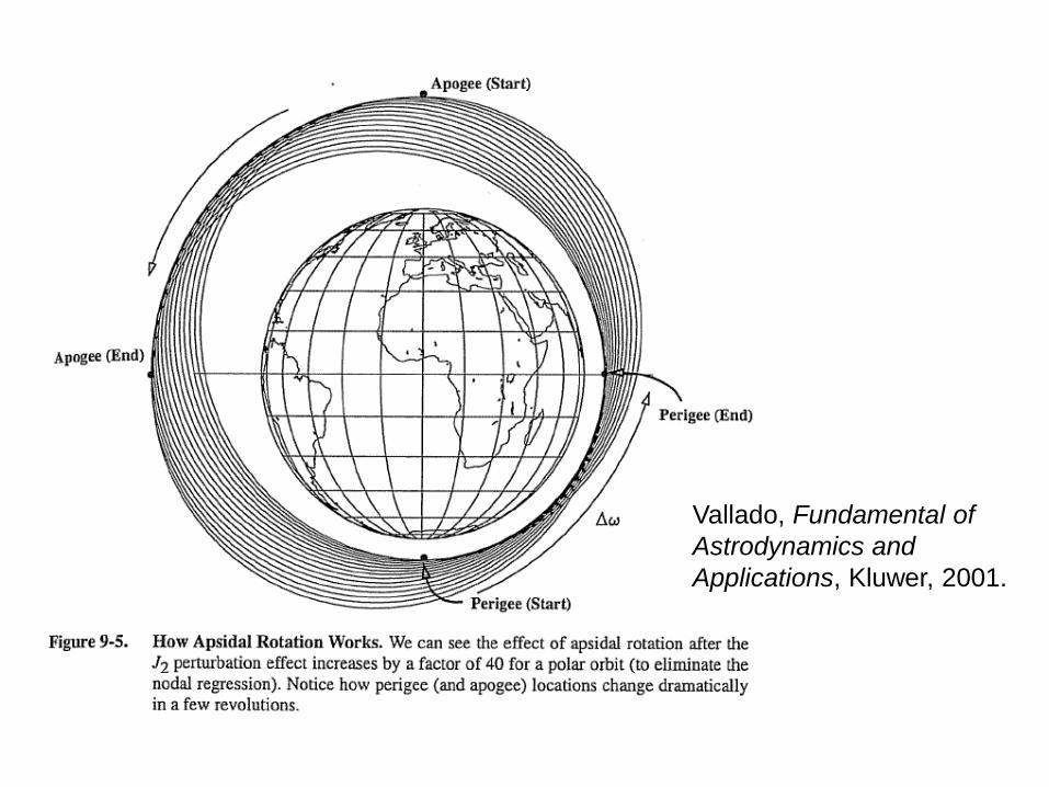
Vallado Fundamental of
Astrodynamics and
Applications Kluwer 2001
30
Exploitation Molniya Orbits
A geostationary satellite cannot view effectively the far
northern latitudes into which Russian territory extends
(+ costly plane change maneuver for the launch vehicle )
Molniya telecommunications satellites are launched from
Plesetsk (628ordmN) into 63ordm inclination orbits having a
period of 12 hours
3
2 the apse line is 53000km longellip
aT
422 Non-spherical Earth
31
Analytic Propagators in STK 2-body J2
2-body constant orbital elements
J2 accounts for secular variations in the orbit elements
due to Earth oblateness periodic variations are
neglected
423 J2 propagator in STK
32
J2 Propagator Underlying Equations
423 J2 propagator in STK
33
2-body and J2 Propagators Applied to ISS
Two-body propagator J2 propagator
423 J2 propagator in STK
34
HPOP and J2 Propagators Applied to ISS
Nodal regression of the ISS
35
Effects of Atmospheric Drag Semi-Major Axis
2a
Lecture 2
2
2
2
2
aa
gt0
Because drag causes the dissipation of mechanical energy
from the system the semimajor axis contracts
424 Atmospheric drag
Drag paradox the effect of atmospheric drag is to increase
the satellite speed and kinetic energy
36
Effects of Atmospheric Drag Semi-Major Axis
21 10
2 2D r D
A AN R T C v C
m m a
0D
Aa a C
m
2
Df i f i
C Aa a t t
m
is assumed constant
424 Atmospheric drag
3
22 Resin 1 cos
1
aa T e
e
Circular orbit
37
Effects of Atmospheric Drag Orbit Plane
2
2sin(1 )
sin 1 cos
Na e
i e
2
2cos(1 )
1 cos
Na ei
e
The orientation of the orbit plane is not changed by drag
424 Atmospheric drag
38
Effects of Atmospheric Drag Apogee Perigee
Apogee height changes drastically perigee height remains
relatively constant
424 Atmospheric drag
Vallado Fundamental of Astrodynamics and Applications Kluwer 2001
39
Effects of Atmospheric Drag Eccentricity
Vallado Fundamental of Astrodynamics and Applications Kluwer 2001
424 Atmospheric drag
40
Early Reentry of Skylab (1979)
Increased solar activity which
increased drag on Skylab led to
an early reentry
Earth reentry footprint could not
be accurately predicted (due to
tumbling and other parameters)
Debris was found around
Esperance (31ndash34degS 122ndash
126degE) The Shire of Esperance
fined the United States $400 for
littering a fine which to this day
remains unpaid
424 Atmospheric drag
41
Lost of ASCA Satellite (2000)
July 15 2000 a strong solar
flare heated the Earthrsquos
atmosphere increasing the
air density to a value 100
times greater than that for
which its ADCS had been
designed to cope The
magnetorquers were unable
to compensate and the
satellite was lost
httpheasarcgsfcnasagovdocsascasafemodehtml
424 Atmospheric drag
42
Effects of Third-Body Perturbations
The only secular perturbations are in the node and in the
perigee
For near-Earth orbits the dominance of the oblateness
dictates that the orbital plane regresses about the polar
axis For higher orbits the regression will be about some
mean pole lying between the Earthrsquos pole and the ecliptic
pole
Many geosynchronous satellites launched 30 years ago
now have inclinations of up to plusmn15ordm collision avoidance
as the satellites drift back through the GEO belt
425 Third-body perturbations
43
Effects of Third-Body Perturbations
Vallado Fundamental of Astrodynamics and Applications Kluwer 2001
The Sunrsquos attraction
tends to turn the
satellite ring into the
ecliptic The orbit
precesses about the
pole of the ecliptic
425 Third-body perturbations
44
STK Analytic Propagator (SGP4)
The J2 propagator does not include drag
SGP4 which stands for Simplified General Perturbations
Satellite Orbit Model 4 is a NASANORAD algorithm
426 SGP4 propagator in STK
45
STK Analytic Propagator (SGP4)
Several assumptions propagation valid for short durations
(3-10 days)
TLE data should be used as the input (see Lecture 03)
It considers secular and periodic variations due to Earth
oblateness solar and lunar gravitational effects and
orbital decay using a drag model
426 SGP4 propagator in STK
46
SGP4 Applied to ISS RAAN
426 SGP4 propagator in STK
47
SGP4 Applied to ISS Semi-Major Axis
426 SGP4 propagator in STK
48
Further Reading on the Web Site
426 SGP4 propagator in STK
49
Effects of Solar Radiation Pressure
The effects are usually small for most satellites
Satellites with very low mass and large surface area are
more affected
427 Solar radiation pressure
Vallado Fundamental of
Astrodynamics and
Applications Kluwer
2001
51
Secular Effects Orders of Magnitude
Vallado Fundamental of Astrodynamics and Applications Kluwer 2001
52
Periodic Effects Orders of Magnitude
Vallado Fundamental of Astrodynamics and Applications Kluwer 2001
53
4 Non-Keplerian Motion
2
2
(1 )
sin
sin 1 cos
a e
N
i e
43 Numerical methods
431 Orbit prediction
432 Numerical integration
433 Single-step methods Runge-Kutta
434 Multi-step methods
435 Integrator and step size selection
436 ISS example
nt 1nt
r
54
2-body analytic propagator (constant orbital elements)
J2 analytic propagator (secular variations in the orbit
elements due to Earth oblateness
HPOP numerical integration of the equations of motion
(periodic and secular effects included)
STK Propagators
431 Orbit prediction
Accurate
Versatile
Errors accumulation
for long intervals
Computationally
intensive
55
Real-Life Example German Aerospace Agency
431 Orbit prediction
56
Real-Life Example German Aerospace Agency
57
Further Reading on the Web Site
431 Orbit prediction
58
Real-Life Example Envisat
httpnngesocesadeenvisat
ENVpredhtml
431 Orbit prediction
Why do the
predictions degrade
for lower altitudes
60
NASA began the first complex numerical integrations
during the late 1960s and early 1970s
Did you Know
1969 1968
431 Orbit prediction
61
What is Numerical Integration
1n nt t t
3 perturbedr
r r a
Given
Compute
( ) ( )n nt tr r
1 1( ) ( )n nt t r r
432 Numerical integration
62
State-Space Formulation
3 perturbedr
r r a
( )f tu u
ru
r
6-dimensional
state vector
432 Numerical integration
63
How to Perform Numerical Integration
2( )( ) ( ) ( ) ( ) ( )
2
ss
n n n n n s
h hf t h f t hf t f t f t R
s
Taylor series expansion
( )ntu
1( )nt u
432 Numerical integration
64
First-Order Taylor Approximation (Euler)
1
( ) ( ) ( )
( )
n n n
n n n n
t t t t t
t f t
u u u
u u uEuler step
0 1 2 3 4 5 60
5
10
15
20
25
30
35
40
Time t (s)
x(t
)=t2
Exact solution
The stepsize has to be extremely
small for accurate predictions
and it is necessary to develop
more effective algorithms
along the tangent
432 Numerical integration
65
Numerical Integration Methods
1 1 1
1 0
m m
n j n j j n j
j j
t
u u u
0 0
Implicit the solution method becomes
iterative in the nonlinear case
0 0 Explicit un+1 can be deduced directly from
the results at the previous time steps
=0
for 1
j j
j
Single-step the system at time tn+1
only depends on the previous state tn
State vector
0
for 1
j j
j
Multi-step the system at time tn+1 depends
several previous states tntn-1etc
432 Numerical integration
66
Examples Implicit vs Explicit
Trapezoidal rule (implicit)
nt 1nt
Euler forward (explicit)
nt 1nt
Euler backward (implicit)
nt 1nt
1n n nt u u u
1 1n n nt u u u
1
12
n n
n n t
u uu u
r
r
r
432 Numerical integration
67
A variety of methods has been applied in astrodynamics
Each of these methods has its own advantages and
drawbacks
Accuracy what is the order of the integration scheme
Efficiency how many function calls
Versatility can it be applied to a wide range of problems
Complexity is it easy to implement and use
Step size automatic step size control
Why Different Methods
431 Orbit prediction
68
Runge-Kutta Family Single-Step
Perhaps the most well-known numerical integrator
Difference with traditional Taylor series integrators the RK
family only requires the first derivative but several
evaluations are needed to move forward one step in time
Different variants explicit embedded etc
433 Single-step methods Runge-Kutta
69
Runge-Kutta Family Single-Step
with ( ) ( )t f tu u 0 0( )t u u
1
1
s
n n i i
i
t b
u u k
1 1
1
1
2
n n
i
i n ij j n i
j
f t c t
f t a t c t i s
k u
k u k
Slopes at
various points
within the
integration step
433 Single-step methods Runge-Kutta
70
Runge-Kutta Family Single-Step
Butcher Tableau
The Runge-Kutta methods are fully described by the
coefficients
c1
c2
cs
a21
as1
b1
as2
b2
ass-1
bs-1 hellip
hellip
hellip hellip hellip
bs
1
1
1
1
1
0
s
i
i
i
i ij
j
b
c
c a
433 Single-step methods Runge-Kutta
71
RK4 (Explicit)
1 2 3 41
2 2
6n n t
k k k ku u
Butcher Tableau
1
2 1
3 2
4 3
2 2
2 2
n n
n n
n n
n n
f t
t tf t
t tf t
f t t t
k u
k u k
k u k
k u k
433 Single-step methods Runge-Kutta
72
RK4 (Explicit)
1 2 3 41
2 2
6n n t
k k k ku u
1
2 1
3 2
4 3
2 2
2 2
n n
n n
n n
n n
f t
t tf t
t tf t
f t t t
k u
k u k
k u k
k u k
Slope at the beginning
Slope at the midpoint (k1 is
used to determine the value
of u Euler)
Slope at the midpoint (k2 is
now used)
Slope at the end
Estimated slope
(weighted average)
433 Single-step methods Runge-Kutta
73
RK4 (Explicit)
nt 2nt t nt t
1k3k
2k
4k
Estimate at new
time
u
433 Single-step methods Runge-Kutta
74
RK4 (Explicit)
The local truncation error for a 4th order RK is O(h5)
The accuracy is comparable to that of a 4th order Taylor
series but the Runge-Kutta method avoids the
calculation of higher-order derivatives
Easy to use and implement
The step size is fixed
433 Single-step methods Runge-Kutta
75
RK4 in STK
433 Single-step methods Runge-Kutta
76
Embedded Methods
They produce an estimate of the local truncation error
adjust the step size to keep local truncation errors
within some tolerances
This is done by having two methods in the tableau one with
order p and one with order p+1 with the same set of
function evaluations
( 1) ( 1) ( 1)
1
1
sp p p
n n i i
i
t b
u u k
( ) ( ) ( )
1
1
sp p p
n n i i
i
t b
u u k
433 Single-step methods Runge-Kutta
77
Embedded Methods
The two different approximations for the solution at each
step are compared
If the two answers are in close agreement the approximation is
accepted
If the two answers do not agree to a specified accuracy the step
size is reduced
If the answers agree to more significant digits than required the
step size is increased
433 Single-step methods Runge-Kutta
78
Ode45 in Matlab Simulink
Runge-Kutta (45) pair of Dormand and Prince
Variable step size
Matlab help This should be the first solver you try
433 Single-step methods Runge-Kutta
79
Ode45 in Matlab Simulink
edit ode45
433 Single-step methods Runge-Kutta
80
Ode45 in Matlab Simulink
Be very careful with the default parameters
options = odeset(RelTol1e-8AbsTol1e-8)
433 Single-step methods Runge-Kutta
81
RKF 7(8) Default Method in STK
Runge-Kutta-Fehlberg integration method of 7th order
with 8th order error control for the integration step size
433 Single-step methods Runge-Kutta
83
Multi-Step Methods (Predictor-Corrector)
They estimate the state over time using previously
determined back values of the solution
Unlike RK methods they only perform one evaluation for
each step forward but they usually have a predictor and a
corrector formula
Adams() ndash Bashforth - Moulton Gauss - Jackson
() The first with Le Verrier to predict the existence and position of Neptune
434 Multi-step methods
84
Multi-Step Methods Principle
( ) ( )t f tu u1
1( ) ( ) ( ) n
n
t
n nt
t t f t dt
u u u
unknown
Replace it by a
polynomial that
interpolates the
previous values Four function values
interpolated by a
third-order polynomial
t
u
434 Multi-step methods
85
Multi-Step Methods Initiation
with ( ) ( )t f tu u 0 0( )t u u
What is the inherent problem
t
u
434 Multi-step methods
86
Multi-Step Methods Initiation
Because these methods require back values they are not
self-starting
One may for instance use of a single-step method to
compute the first four values
434 Multi-step methods
87
Gauss-Jackson in STK
One of the most recommendable fixed-stepsize multistep
methods for orbit computations
88
Integrator Selection
435 Integrator and step size selection
Montenbruck and Gill
Satellite orbits Springer
2000
89
Integrator Selection
Pros
Very fast
Cons
Special starting procedure
Fixed time steps
Error control
Pros
Plug and play
Error control
Cons
Slower
Multi-step Single step
435 Integrator and step size selection
90
Why is the Step Size So Critical
Theoretical arguments
1 The accuracy and the stability of the algorithm are
directly related to the step size
2 Nonlinear equations of motion
Data for Landsat 4 and 6 in circular orbits around 800km
indicates that a one-minute step size yields about 47m
error
A three-minute step size produces about a 900m error
435 Integrator and step size selection
91
Why is the Step Size So Critical
More practical arguments
1 The computation time is directly related to the
step size
2 The particular choice of step size depends on the
most rapidly varying component in the disturbing
functions (eg 50 x 50 gravity field)
435 Integrator and step size selection
92
Appropriate Step Size
The problem of determining an appropriate step size is a
challenge in any numerical process
Fixed step size (rule of thumb for standard
applications)
But an algorithm with variable step size is really
helpful The step size is chosen in such a way that
each step contributes uniformly to the total integration
error
100
orbitTt
435 Integrator and step size selection
93
Three Examples XMM OUFTI-1 ISS
Can you plot the step size vs true anomaly
435 Integrator and step size selection
94
XMM Report in STK
435 Integrator and step size selection
95
XMM (e~08)
0 50 100 150 200 250 300 350 4000
1000
2000
3000
4000
5000
6000
True anomaly (deg)
Ste
p s
ize
(s)
435 Integrator and step size selection
96
ISS(e~0)
435 Integrator and step size selection
0 50 100 150 200 250 300 350 40030
35
40
45
50
55
60
65
70
True anomaly (deg)
Ste
p s
ize
(s)
97
ldquoDifficultrdquo Orbits
Automatic time step is especially nice on highly eccentric
orbits (Molniya XMM) These orbits are best computed
using variable step sizes to maintain some given level of
accuracy
Without this variable step size we waste a lot of time near
apoapsis when the integration is taking too small a step
Likewise the integrator may not be using a small enough step
size at periapsis where the satellite is traveling fast
435 Integrator and step size selection
98
HPOP Propagator ISS Example
1 Earthrsquos oblateness only
2 Drag only
3 Sun and moon only
4 SRP only
5 All together
436 ISS example
99
Earthrsquos Oblateness Only Ω
HPOP
J2
2-body
436 ISS example
100
Earthrsquos Oblateness Only i Ω a
HPOP with central body (20 + WGS84_EGM96)
(without dragSRPSun and Moon)
436 ISS example
101
Drag Only i Ω a
HPOP with drag ndash Harris Priester
(without oblatenessSRPSun and Moon)
436 ISS example
102
Drag Relationship with Eclipses
103
SRP Only i Ω a
HPOP with SRP
(without oblatenessdragSun and Moon)
436 ISS example
104
SRP Relationship with Eclipses
105
All Perturbations Together
436 ISS example
106
4 Non-Keplerian Motion
2
2
(1 )
sin
sin 1 cos
a e
N
i e
44 Geostationary satellites
107
Practical Example GEO Satellites
Nice illustration of
1 Perturbations of the 2-body problem
2 Secular and periodic contributions
3 Accuracy required by practical applications
4 The need for orbit correction and thrust forces
And it is a real-life example (telecommunications
meteorology)
44 GEO satellites
108
Three Main Perturbations for GEO Satellites
44 GEO satellites
1 Non-spherical Earth
2 SRP
3 Sun and Moon
109
Station Keeping of GEO Satellites
The effect of the perturbations is to cause the spacecraft
to drift away from its nominal station If the drift was
allowed to build up unchecked the spacecraft could
become useless
A station-keeping box is defined by a longitude and a
maximum authorized distance for satellite excursions in
longitude and latitude
For instance TC2 -8ordm plusmn 007ordm EW plusmn 005ordm NS
44 GEO satellites
110
East-West and North-South Drift
44 GEO satellites
NS drift
EW drift
What are the perturbations generating these drifts
111
East-West Drift
44 GEO satellites
A GEO satellite drifts in longitude due to the influence of
two main perturbations
1 The elliptic nature of the Earthrsquos equatorial cross-
section J22 (and not from the NS oblateness J2)
2
ΔV
ΔV vsat
vsat SRP
112
East-West Drift due to Equatorial Ellipticity
44 GEO satellites
113
East-West Drift due to Equatorial Ellipticity
44 GEO satellites
114
East-West Drift HPOP (20) vs HPOP (22)
44 GEO satellites
115
East-West Drift Stable Equilibirum
HPOP with 22
(without Sun and moonSRPdrag)
116
East-West Drift Stable Equilibirum
HPOP with 22
(without Sun and moonSRPdrag)
117
East-West Drift Stable Equilibirum
HPOP with 22
(without Sun and moonSRPdrag)
118
North-South Drift
The perturbations caused by the Sun and the Moon are
predominantly out-of-plane effects causing a change in
the inclination and in the right ascension of the orbit
ascending node
Similar effects on the orbit to those of the Earthrsquos
oblateness (but here with respect to the ecliptic)
A GEO satellite therefore drifts in latitude with a
fundamental period equal to the orbit period
119
North-South Drift
Period
HPOP with Sun and Moon
(without oblatenessSRPdrag)
120
North-South Drift
Period
HPOP with Sun and Moon
(without oblatenessSRPdrag)
121
Thrust Forces for Stationkeeping
GEO spacecraft require continual stationkeeping to stay
within the authorized box using onboard thrusters
44 GEO satellites
122
42 ANALYTIC TREATMENT
421 Variation of parameters
422 Non-spherical Earth
423 J2 propagator in STK
424 Atmospheric drag
425 Third-body perturbations
426 SGP4 propagator in STK
427 Solar radiation pressure
4 Non-Keplerian Motion
43 NUMERICAL METHODS
431 Orbit prediction
432 Numerical integration
433 Single-step methods Runge-Kutta
434 Multi-step methods
435 Integrator and step size selection
436 ISS example
44 GEOSTATIONARY SATELLITES
Gaeumltan Kerschen
Space Structures amp
Systems Lab (S3L)
4B Non-Keplerian Motion
Astrodynamics (AERO0024)
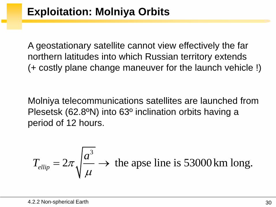
30
Exploitation Molniya Orbits
A geostationary satellite cannot view effectively the far
northern latitudes into which Russian territory extends
(+ costly plane change maneuver for the launch vehicle )
Molniya telecommunications satellites are launched from
Plesetsk (628ordmN) into 63ordm inclination orbits having a
period of 12 hours
3
2 the apse line is 53000km longellip
aT
422 Non-spherical Earth
31
Analytic Propagators in STK 2-body J2
2-body constant orbital elements
J2 accounts for secular variations in the orbit elements
due to Earth oblateness periodic variations are
neglected
423 J2 propagator in STK
32
J2 Propagator Underlying Equations
423 J2 propagator in STK
33
2-body and J2 Propagators Applied to ISS
Two-body propagator J2 propagator
423 J2 propagator in STK
34
HPOP and J2 Propagators Applied to ISS
Nodal regression of the ISS
35
Effects of Atmospheric Drag Semi-Major Axis
2a
Lecture 2
2
2
2
2
aa
gt0
Because drag causes the dissipation of mechanical energy
from the system the semimajor axis contracts
424 Atmospheric drag
Drag paradox the effect of atmospheric drag is to increase
the satellite speed and kinetic energy
36
Effects of Atmospheric Drag Semi-Major Axis
21 10
2 2D r D
A AN R T C v C
m m a
0D
Aa a C
m
2
Df i f i
C Aa a t t
m
is assumed constant
424 Atmospheric drag
3
22 Resin 1 cos
1
aa T e
e
Circular orbit
37
Effects of Atmospheric Drag Orbit Plane
2
2sin(1 )
sin 1 cos
Na e
i e
2
2cos(1 )
1 cos
Na ei
e
The orientation of the orbit plane is not changed by drag
424 Atmospheric drag
38
Effects of Atmospheric Drag Apogee Perigee
Apogee height changes drastically perigee height remains
relatively constant
424 Atmospheric drag
Vallado Fundamental of Astrodynamics and Applications Kluwer 2001
39
Effects of Atmospheric Drag Eccentricity
Vallado Fundamental of Astrodynamics and Applications Kluwer 2001
424 Atmospheric drag
40
Early Reentry of Skylab (1979)
Increased solar activity which
increased drag on Skylab led to
an early reentry
Earth reentry footprint could not
be accurately predicted (due to
tumbling and other parameters)
Debris was found around
Esperance (31ndash34degS 122ndash
126degE) The Shire of Esperance
fined the United States $400 for
littering a fine which to this day
remains unpaid
424 Atmospheric drag
41
Lost of ASCA Satellite (2000)
July 15 2000 a strong solar
flare heated the Earthrsquos
atmosphere increasing the
air density to a value 100
times greater than that for
which its ADCS had been
designed to cope The
magnetorquers were unable
to compensate and the
satellite was lost
httpheasarcgsfcnasagovdocsascasafemodehtml
424 Atmospheric drag
42
Effects of Third-Body Perturbations
The only secular perturbations are in the node and in the
perigee
For near-Earth orbits the dominance of the oblateness
dictates that the orbital plane regresses about the polar
axis For higher orbits the regression will be about some
mean pole lying between the Earthrsquos pole and the ecliptic
pole
Many geosynchronous satellites launched 30 years ago
now have inclinations of up to plusmn15ordm collision avoidance
as the satellites drift back through the GEO belt
425 Third-body perturbations
43
Effects of Third-Body Perturbations
Vallado Fundamental of Astrodynamics and Applications Kluwer 2001
The Sunrsquos attraction
tends to turn the
satellite ring into the
ecliptic The orbit
precesses about the
pole of the ecliptic
425 Third-body perturbations
44
STK Analytic Propagator (SGP4)
The J2 propagator does not include drag
SGP4 which stands for Simplified General Perturbations
Satellite Orbit Model 4 is a NASANORAD algorithm
426 SGP4 propagator in STK
45
STK Analytic Propagator (SGP4)
Several assumptions propagation valid for short durations
(3-10 days)
TLE data should be used as the input (see Lecture 03)
It considers secular and periodic variations due to Earth
oblateness solar and lunar gravitational effects and
orbital decay using a drag model
426 SGP4 propagator in STK
46
SGP4 Applied to ISS RAAN
426 SGP4 propagator in STK
47
SGP4 Applied to ISS Semi-Major Axis
426 SGP4 propagator in STK
48
Further Reading on the Web Site
426 SGP4 propagator in STK
49
Effects of Solar Radiation Pressure
The effects are usually small for most satellites
Satellites with very low mass and large surface area are
more affected
427 Solar radiation pressure
Vallado Fundamental of
Astrodynamics and
Applications Kluwer
2001
51
Secular Effects Orders of Magnitude
Vallado Fundamental of Astrodynamics and Applications Kluwer 2001
52
Periodic Effects Orders of Magnitude
Vallado Fundamental of Astrodynamics and Applications Kluwer 2001
53
4 Non-Keplerian Motion
2
2
(1 )
sin
sin 1 cos
a e
N
i e
43 Numerical methods
431 Orbit prediction
432 Numerical integration
433 Single-step methods Runge-Kutta
434 Multi-step methods
435 Integrator and step size selection
436 ISS example
nt 1nt
r
54
2-body analytic propagator (constant orbital elements)
J2 analytic propagator (secular variations in the orbit
elements due to Earth oblateness
HPOP numerical integration of the equations of motion
(periodic and secular effects included)
STK Propagators
431 Orbit prediction
Accurate
Versatile
Errors accumulation
for long intervals
Computationally
intensive
55
Real-Life Example German Aerospace Agency
431 Orbit prediction
56
Real-Life Example German Aerospace Agency
57
Further Reading on the Web Site
431 Orbit prediction
58
Real-Life Example Envisat
httpnngesocesadeenvisat
ENVpredhtml
431 Orbit prediction
Why do the
predictions degrade
for lower altitudes
60
NASA began the first complex numerical integrations
during the late 1960s and early 1970s
Did you Know
1969 1968
431 Orbit prediction
61
What is Numerical Integration
1n nt t t
3 perturbedr
r r a
Given
Compute
( ) ( )n nt tr r
1 1( ) ( )n nt t r r
432 Numerical integration
62
State-Space Formulation
3 perturbedr
r r a
( )f tu u
ru
r
6-dimensional
state vector
432 Numerical integration
63
How to Perform Numerical Integration
2( )( ) ( ) ( ) ( ) ( )
2
ss
n n n n n s
h hf t h f t hf t f t f t R
s
Taylor series expansion
( )ntu
1( )nt u
432 Numerical integration
64
First-Order Taylor Approximation (Euler)
1
( ) ( ) ( )
( )
n n n
n n n n
t t t t t
t f t
u u u
u u uEuler step
0 1 2 3 4 5 60
5
10
15
20
25
30
35
40
Time t (s)
x(t
)=t2
Exact solution
The stepsize has to be extremely
small for accurate predictions
and it is necessary to develop
more effective algorithms
along the tangent
432 Numerical integration
65
Numerical Integration Methods
1 1 1
1 0
m m
n j n j j n j
j j
t
u u u
0 0
Implicit the solution method becomes
iterative in the nonlinear case
0 0 Explicit un+1 can be deduced directly from
the results at the previous time steps
=0
for 1
j j
j
Single-step the system at time tn+1
only depends on the previous state tn
State vector
0
for 1
j j
j
Multi-step the system at time tn+1 depends
several previous states tntn-1etc
432 Numerical integration
66
Examples Implicit vs Explicit
Trapezoidal rule (implicit)
nt 1nt
Euler forward (explicit)
nt 1nt
Euler backward (implicit)
nt 1nt
1n n nt u u u
1 1n n nt u u u
1
12
n n
n n t
u uu u
r
r
r
432 Numerical integration
67
A variety of methods has been applied in astrodynamics
Each of these methods has its own advantages and
drawbacks
Accuracy what is the order of the integration scheme
Efficiency how many function calls
Versatility can it be applied to a wide range of problems
Complexity is it easy to implement and use
Step size automatic step size control
Why Different Methods
431 Orbit prediction
68
Runge-Kutta Family Single-Step
Perhaps the most well-known numerical integrator
Difference with traditional Taylor series integrators the RK
family only requires the first derivative but several
evaluations are needed to move forward one step in time
Different variants explicit embedded etc
433 Single-step methods Runge-Kutta
69
Runge-Kutta Family Single-Step
with ( ) ( )t f tu u 0 0( )t u u
1
1
s
n n i i
i
t b
u u k
1 1
1
1
2
n n
i
i n ij j n i
j
f t c t
f t a t c t i s
k u
k u k
Slopes at
various points
within the
integration step
433 Single-step methods Runge-Kutta
70
Runge-Kutta Family Single-Step
Butcher Tableau
The Runge-Kutta methods are fully described by the
coefficients
c1
c2
cs
a21
as1
b1
as2
b2
ass-1
bs-1 hellip
hellip
hellip hellip hellip
bs
1
1
1
1
1
0
s
i
i
i
i ij
j
b
c
c a
433 Single-step methods Runge-Kutta
71
RK4 (Explicit)
1 2 3 41
2 2
6n n t
k k k ku u
Butcher Tableau
1
2 1
3 2
4 3
2 2
2 2
n n
n n
n n
n n
f t
t tf t
t tf t
f t t t
k u
k u k
k u k
k u k
433 Single-step methods Runge-Kutta
72
RK4 (Explicit)
1 2 3 41
2 2
6n n t
k k k ku u
1
2 1
3 2
4 3
2 2
2 2
n n
n n
n n
n n
f t
t tf t
t tf t
f t t t
k u
k u k
k u k
k u k
Slope at the beginning
Slope at the midpoint (k1 is
used to determine the value
of u Euler)
Slope at the midpoint (k2 is
now used)
Slope at the end
Estimated slope
(weighted average)
433 Single-step methods Runge-Kutta
73
RK4 (Explicit)
nt 2nt t nt t
1k3k
2k
4k
Estimate at new
time
u
433 Single-step methods Runge-Kutta
74
RK4 (Explicit)
The local truncation error for a 4th order RK is O(h5)
The accuracy is comparable to that of a 4th order Taylor
series but the Runge-Kutta method avoids the
calculation of higher-order derivatives
Easy to use and implement
The step size is fixed
433 Single-step methods Runge-Kutta
75
RK4 in STK
433 Single-step methods Runge-Kutta
76
Embedded Methods
They produce an estimate of the local truncation error
adjust the step size to keep local truncation errors
within some tolerances
This is done by having two methods in the tableau one with
order p and one with order p+1 with the same set of
function evaluations
( 1) ( 1) ( 1)
1
1
sp p p
n n i i
i
t b
u u k
( ) ( ) ( )
1
1
sp p p
n n i i
i
t b
u u k
433 Single-step methods Runge-Kutta
77
Embedded Methods
The two different approximations for the solution at each
step are compared
If the two answers are in close agreement the approximation is
accepted
If the two answers do not agree to a specified accuracy the step
size is reduced
If the answers agree to more significant digits than required the
step size is increased
433 Single-step methods Runge-Kutta
78
Ode45 in Matlab Simulink
Runge-Kutta (45) pair of Dormand and Prince
Variable step size
Matlab help This should be the first solver you try
433 Single-step methods Runge-Kutta
79
Ode45 in Matlab Simulink
edit ode45
433 Single-step methods Runge-Kutta
80
Ode45 in Matlab Simulink
Be very careful with the default parameters
options = odeset(RelTol1e-8AbsTol1e-8)
433 Single-step methods Runge-Kutta
81
RKF 7(8) Default Method in STK
Runge-Kutta-Fehlberg integration method of 7th order
with 8th order error control for the integration step size
433 Single-step methods Runge-Kutta
83
Multi-Step Methods (Predictor-Corrector)
They estimate the state over time using previously
determined back values of the solution
Unlike RK methods they only perform one evaluation for
each step forward but they usually have a predictor and a
corrector formula
Adams() ndash Bashforth - Moulton Gauss - Jackson
() The first with Le Verrier to predict the existence and position of Neptune
434 Multi-step methods
84
Multi-Step Methods Principle
( ) ( )t f tu u1
1( ) ( ) ( ) n
n
t
n nt
t t f t dt
u u u
unknown
Replace it by a
polynomial that
interpolates the
previous values Four function values
interpolated by a
third-order polynomial
t
u
434 Multi-step methods
85
Multi-Step Methods Initiation
with ( ) ( )t f tu u 0 0( )t u u
What is the inherent problem
t
u
434 Multi-step methods
86
Multi-Step Methods Initiation
Because these methods require back values they are not
self-starting
One may for instance use of a single-step method to
compute the first four values
434 Multi-step methods
87
Gauss-Jackson in STK
One of the most recommendable fixed-stepsize multistep
methods for orbit computations
88
Integrator Selection
435 Integrator and step size selection
Montenbruck and Gill
Satellite orbits Springer
2000
89
Integrator Selection
Pros
Very fast
Cons
Special starting procedure
Fixed time steps
Error control
Pros
Plug and play
Error control
Cons
Slower
Multi-step Single step
435 Integrator and step size selection
90
Why is the Step Size So Critical
Theoretical arguments
1 The accuracy and the stability of the algorithm are
directly related to the step size
2 Nonlinear equations of motion
Data for Landsat 4 and 6 in circular orbits around 800km
indicates that a one-minute step size yields about 47m
error
A three-minute step size produces about a 900m error
435 Integrator and step size selection
91
Why is the Step Size So Critical
More practical arguments
1 The computation time is directly related to the
step size
2 The particular choice of step size depends on the
most rapidly varying component in the disturbing
functions (eg 50 x 50 gravity field)
435 Integrator and step size selection
92
Appropriate Step Size
The problem of determining an appropriate step size is a
challenge in any numerical process
Fixed step size (rule of thumb for standard
applications)
But an algorithm with variable step size is really
helpful The step size is chosen in such a way that
each step contributes uniformly to the total integration
error
100
orbitTt
435 Integrator and step size selection
93
Three Examples XMM OUFTI-1 ISS
Can you plot the step size vs true anomaly
435 Integrator and step size selection
94
XMM Report in STK
435 Integrator and step size selection
95
XMM (e~08)
0 50 100 150 200 250 300 350 4000
1000
2000
3000
4000
5000
6000
True anomaly (deg)
Ste
p s
ize
(s)
435 Integrator and step size selection
96
ISS(e~0)
435 Integrator and step size selection
0 50 100 150 200 250 300 350 40030
35
40
45
50
55
60
65
70
True anomaly (deg)
Ste
p s
ize
(s)
97
ldquoDifficultrdquo Orbits
Automatic time step is especially nice on highly eccentric
orbits (Molniya XMM) These orbits are best computed
using variable step sizes to maintain some given level of
accuracy
Without this variable step size we waste a lot of time near
apoapsis when the integration is taking too small a step
Likewise the integrator may not be using a small enough step
size at periapsis where the satellite is traveling fast
435 Integrator and step size selection
98
HPOP Propagator ISS Example
1 Earthrsquos oblateness only
2 Drag only
3 Sun and moon only
4 SRP only
5 All together
436 ISS example
99
Earthrsquos Oblateness Only Ω
HPOP
J2
2-body
436 ISS example
100
Earthrsquos Oblateness Only i Ω a
HPOP with central body (20 + WGS84_EGM96)
(without dragSRPSun and Moon)
436 ISS example
101
Drag Only i Ω a
HPOP with drag ndash Harris Priester
(without oblatenessSRPSun and Moon)
436 ISS example
102
Drag Relationship with Eclipses
103
SRP Only i Ω a
HPOP with SRP
(without oblatenessdragSun and Moon)
436 ISS example
104
SRP Relationship with Eclipses
105
All Perturbations Together
436 ISS example
106
4 Non-Keplerian Motion
2
2
(1 )
sin
sin 1 cos
a e
N
i e
44 Geostationary satellites
107
Practical Example GEO Satellites
Nice illustration of
1 Perturbations of the 2-body problem
2 Secular and periodic contributions
3 Accuracy required by practical applications
4 The need for orbit correction and thrust forces
And it is a real-life example (telecommunications
meteorology)
44 GEO satellites
108
Three Main Perturbations for GEO Satellites
44 GEO satellites
1 Non-spherical Earth
2 SRP
3 Sun and Moon
109
Station Keeping of GEO Satellites
The effect of the perturbations is to cause the spacecraft
to drift away from its nominal station If the drift was
allowed to build up unchecked the spacecraft could
become useless
A station-keeping box is defined by a longitude and a
maximum authorized distance for satellite excursions in
longitude and latitude
For instance TC2 -8ordm plusmn 007ordm EW plusmn 005ordm NS
44 GEO satellites
110
East-West and North-South Drift
44 GEO satellites
NS drift
EW drift
What are the perturbations generating these drifts
111
East-West Drift
44 GEO satellites
A GEO satellite drifts in longitude due to the influence of
two main perturbations
1 The elliptic nature of the Earthrsquos equatorial cross-
section J22 (and not from the NS oblateness J2)
2
ΔV
ΔV vsat
vsat SRP
112
East-West Drift due to Equatorial Ellipticity
44 GEO satellites
113
East-West Drift due to Equatorial Ellipticity
44 GEO satellites
114
East-West Drift HPOP (20) vs HPOP (22)
44 GEO satellites
115
East-West Drift Stable Equilibirum
HPOP with 22
(without Sun and moonSRPdrag)
116
East-West Drift Stable Equilibirum
HPOP with 22
(without Sun and moonSRPdrag)
117
East-West Drift Stable Equilibirum
HPOP with 22
(without Sun and moonSRPdrag)
118
North-South Drift
The perturbations caused by the Sun and the Moon are
predominantly out-of-plane effects causing a change in
the inclination and in the right ascension of the orbit
ascending node
Similar effects on the orbit to those of the Earthrsquos
oblateness (but here with respect to the ecliptic)
A GEO satellite therefore drifts in latitude with a
fundamental period equal to the orbit period
119
North-South Drift
Period
HPOP with Sun and Moon
(without oblatenessSRPdrag)
120
North-South Drift
Period
HPOP with Sun and Moon
(without oblatenessSRPdrag)
121
Thrust Forces for Stationkeeping
GEO spacecraft require continual stationkeeping to stay
within the authorized box using onboard thrusters
44 GEO satellites
122
42 ANALYTIC TREATMENT
421 Variation of parameters
422 Non-spherical Earth
423 J2 propagator in STK
424 Atmospheric drag
425 Third-body perturbations
426 SGP4 propagator in STK
427 Solar radiation pressure
4 Non-Keplerian Motion
43 NUMERICAL METHODS
431 Orbit prediction
432 Numerical integration
433 Single-step methods Runge-Kutta
434 Multi-step methods
435 Integrator and step size selection
436 ISS example
44 GEOSTATIONARY SATELLITES
Gaeumltan Kerschen
Space Structures amp
Systems Lab (S3L)
4B Non-Keplerian Motion
Astrodynamics (AERO0024)
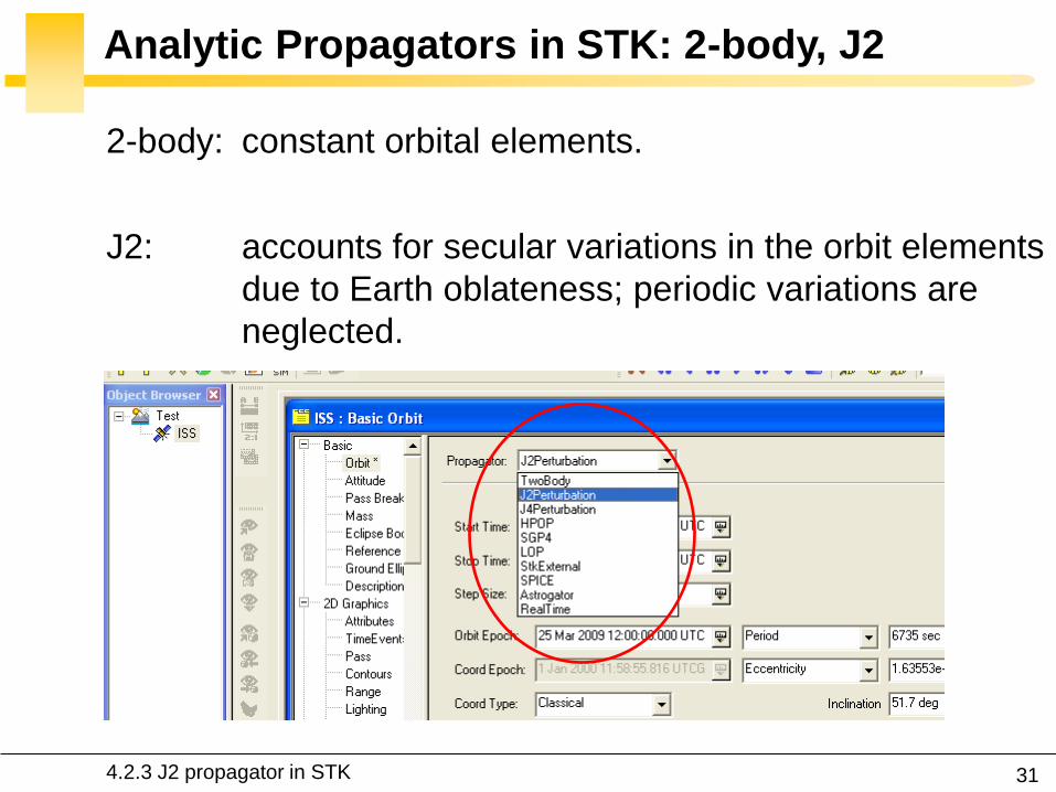
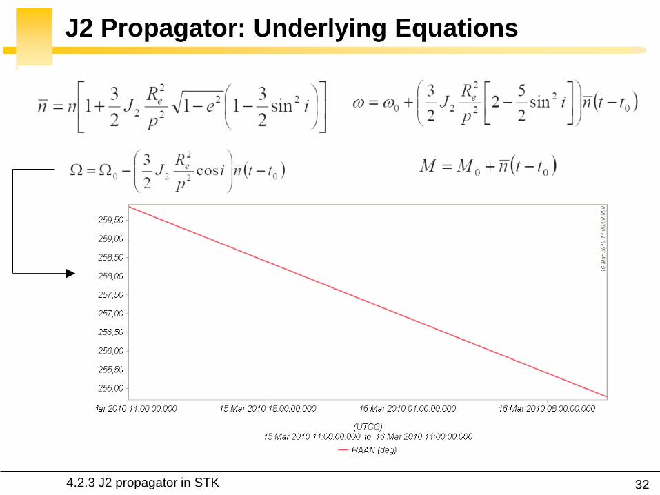
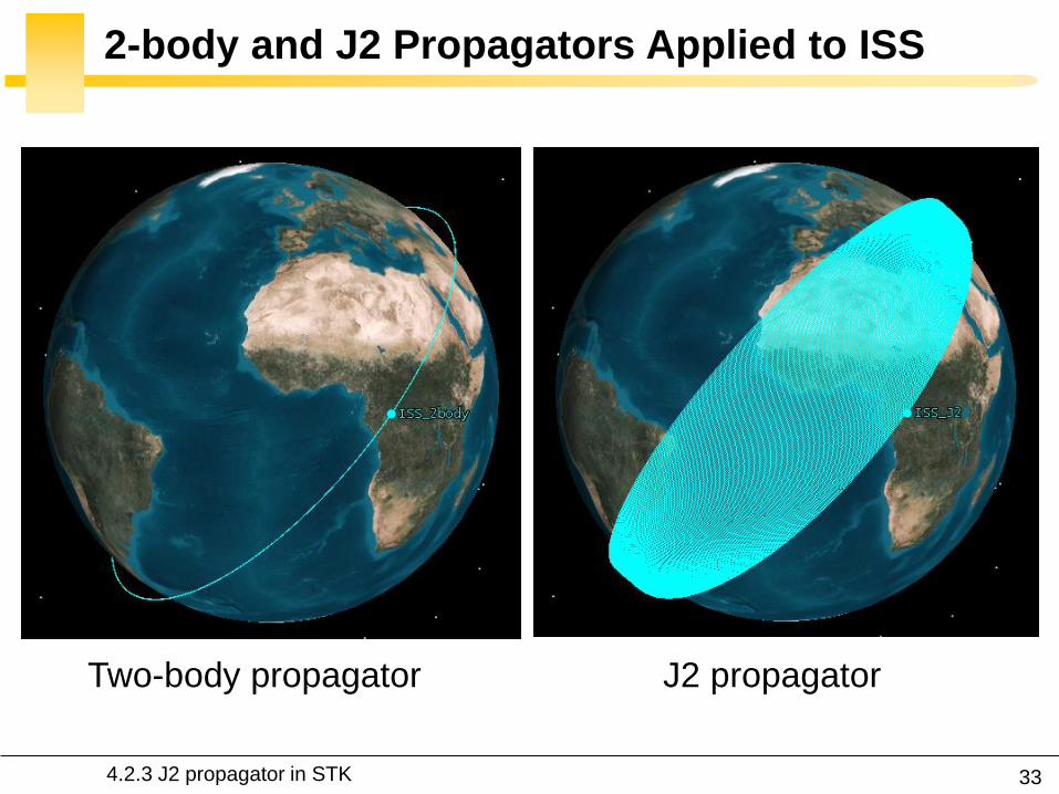
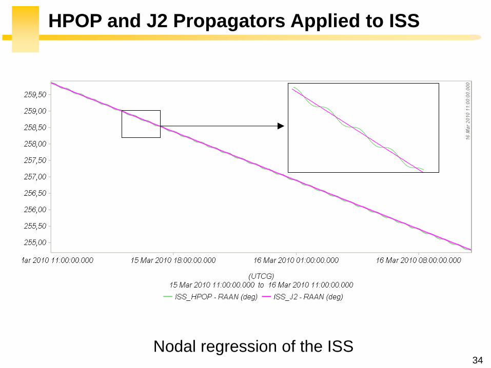
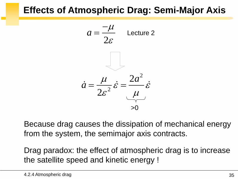
35
Effects of Atmospheric Drag Semi-Major Axis
2a
Lecture 2
2
2
2
2
aa
gt0
Because drag causes the dissipation of mechanical energy
from the system the semimajor axis contracts
424 Atmospheric drag
Drag paradox the effect of atmospheric drag is to increase
the satellite speed and kinetic energy
36
Effects of Atmospheric Drag Semi-Major Axis
21 10
2 2D r D
A AN R T C v C
m m a
0D
Aa a C
m
2
Df i f i
C Aa a t t
m
is assumed constant
424 Atmospheric drag
3
22 Resin 1 cos
1
aa T e
e
Circular orbit
37
Effects of Atmospheric Drag Orbit Plane
2
2sin(1 )
sin 1 cos
Na e
i e
2
2cos(1 )
1 cos
Na ei
e
The orientation of the orbit plane is not changed by drag
424 Atmospheric drag
38
Effects of Atmospheric Drag Apogee Perigee
Apogee height changes drastically perigee height remains
relatively constant
424 Atmospheric drag
Vallado Fundamental of Astrodynamics and Applications Kluwer 2001
39
Effects of Atmospheric Drag Eccentricity
Vallado Fundamental of Astrodynamics and Applications Kluwer 2001
424 Atmospheric drag
40
Early Reentry of Skylab (1979)
Increased solar activity which
increased drag on Skylab led to
an early reentry
Earth reentry footprint could not
be accurately predicted (due to
tumbling and other parameters)
Debris was found around
Esperance (31ndash34degS 122ndash
126degE) The Shire of Esperance
fined the United States $400 for
littering a fine which to this day
remains unpaid
424 Atmospheric drag
41
Lost of ASCA Satellite (2000)
July 15 2000 a strong solar
flare heated the Earthrsquos
atmosphere increasing the
air density to a value 100
times greater than that for
which its ADCS had been
designed to cope The
magnetorquers were unable
to compensate and the
satellite was lost
httpheasarcgsfcnasagovdocsascasafemodehtml
424 Atmospheric drag
42
Effects of Third-Body Perturbations
The only secular perturbations are in the node and in the
perigee
For near-Earth orbits the dominance of the oblateness
dictates that the orbital plane regresses about the polar
axis For higher orbits the regression will be about some
mean pole lying between the Earthrsquos pole and the ecliptic
pole
Many geosynchronous satellites launched 30 years ago
now have inclinations of up to plusmn15ordm collision avoidance
as the satellites drift back through the GEO belt
425 Third-body perturbations
43
Effects of Third-Body Perturbations
Vallado Fundamental of Astrodynamics and Applications Kluwer 2001
The Sunrsquos attraction
tends to turn the
satellite ring into the
ecliptic The orbit
precesses about the
pole of the ecliptic
425 Third-body perturbations
44
STK Analytic Propagator (SGP4)
The J2 propagator does not include drag
SGP4 which stands for Simplified General Perturbations
Satellite Orbit Model 4 is a NASANORAD algorithm
426 SGP4 propagator in STK
45
STK Analytic Propagator (SGP4)
Several assumptions propagation valid for short durations
(3-10 days)
TLE data should be used as the input (see Lecture 03)
It considers secular and periodic variations due to Earth
oblateness solar and lunar gravitational effects and
orbital decay using a drag model
426 SGP4 propagator in STK
46
SGP4 Applied to ISS RAAN
426 SGP4 propagator in STK
47
SGP4 Applied to ISS Semi-Major Axis
426 SGP4 propagator in STK
48
Further Reading on the Web Site
426 SGP4 propagator in STK
49
Effects of Solar Radiation Pressure
The effects are usually small for most satellites
Satellites with very low mass and large surface area are
more affected
427 Solar radiation pressure
Vallado Fundamental of
Astrodynamics and
Applications Kluwer
2001
51
Secular Effects Orders of Magnitude
Vallado Fundamental of Astrodynamics and Applications Kluwer 2001
52
Periodic Effects Orders of Magnitude
Vallado Fundamental of Astrodynamics and Applications Kluwer 2001
53
4 Non-Keplerian Motion
2
2
(1 )
sin
sin 1 cos
a e
N
i e
43 Numerical methods
431 Orbit prediction
432 Numerical integration
433 Single-step methods Runge-Kutta
434 Multi-step methods
435 Integrator and step size selection
436 ISS example
nt 1nt
r
54
2-body analytic propagator (constant orbital elements)
J2 analytic propagator (secular variations in the orbit
elements due to Earth oblateness
HPOP numerical integration of the equations of motion
(periodic and secular effects included)
STK Propagators
431 Orbit prediction
Accurate
Versatile
Errors accumulation
for long intervals
Computationally
intensive
55
Real-Life Example German Aerospace Agency
431 Orbit prediction
56
Real-Life Example German Aerospace Agency
57
Further Reading on the Web Site
431 Orbit prediction
58
Real-Life Example Envisat
httpnngesocesadeenvisat
ENVpredhtml
431 Orbit prediction
Why do the
predictions degrade
for lower altitudes
60
NASA began the first complex numerical integrations
during the late 1960s and early 1970s
Did you Know
1969 1968
431 Orbit prediction
61
What is Numerical Integration
1n nt t t
3 perturbedr
r r a
Given
Compute
( ) ( )n nt tr r
1 1( ) ( )n nt t r r
432 Numerical integration
62
State-Space Formulation
3 perturbedr
r r a
( )f tu u
ru
r
6-dimensional
state vector
432 Numerical integration
63
How to Perform Numerical Integration
2( )( ) ( ) ( ) ( ) ( )
2
ss
n n n n n s
h hf t h f t hf t f t f t R
s
Taylor series expansion
( )ntu
1( )nt u
432 Numerical integration
64
First-Order Taylor Approximation (Euler)
1
( ) ( ) ( )
( )
n n n
n n n n
t t t t t
t f t
u u u
u u uEuler step
0 1 2 3 4 5 60
5
10
15
20
25
30
35
40
Time t (s)
x(t
)=t2
Exact solution
The stepsize has to be extremely
small for accurate predictions
and it is necessary to develop
more effective algorithms
along the tangent
432 Numerical integration
65
Numerical Integration Methods
1 1 1
1 0
m m
n j n j j n j
j j
t
u u u
0 0
Implicit the solution method becomes
iterative in the nonlinear case
0 0 Explicit un+1 can be deduced directly from
the results at the previous time steps
=0
for 1
j j
j
Single-step the system at time tn+1
only depends on the previous state tn
State vector
0
for 1
j j
j
Multi-step the system at time tn+1 depends
several previous states tntn-1etc
432 Numerical integration
66
Examples Implicit vs Explicit
Trapezoidal rule (implicit)
nt 1nt
Euler forward (explicit)
nt 1nt
Euler backward (implicit)
nt 1nt
1n n nt u u u
1 1n n nt u u u
1
12
n n
n n t
u uu u
r
r
r
432 Numerical integration
67
A variety of methods has been applied in astrodynamics
Each of these methods has its own advantages and
drawbacks
Accuracy what is the order of the integration scheme
Efficiency how many function calls
Versatility can it be applied to a wide range of problems
Complexity is it easy to implement and use
Step size automatic step size control
Why Different Methods
431 Orbit prediction
68
Runge-Kutta Family Single-Step
Perhaps the most well-known numerical integrator
Difference with traditional Taylor series integrators the RK
family only requires the first derivative but several
evaluations are needed to move forward one step in time
Different variants explicit embedded etc
433 Single-step methods Runge-Kutta
69
Runge-Kutta Family Single-Step
with ( ) ( )t f tu u 0 0( )t u u
1
1
s
n n i i
i
t b
u u k
1 1
1
1
2
n n
i
i n ij j n i
j
f t c t
f t a t c t i s
k u
k u k
Slopes at
various points
within the
integration step
433 Single-step methods Runge-Kutta
70
Runge-Kutta Family Single-Step
Butcher Tableau
The Runge-Kutta methods are fully described by the
coefficients
c1
c2
cs
a21
as1
b1
as2
b2
ass-1
bs-1 hellip
hellip
hellip hellip hellip
bs
1
1
1
1
1
0
s
i
i
i
i ij
j
b
c
c a
433 Single-step methods Runge-Kutta
71
RK4 (Explicit)
1 2 3 41
2 2
6n n t
k k k ku u
Butcher Tableau
1
2 1
3 2
4 3
2 2
2 2
n n
n n
n n
n n
f t
t tf t
t tf t
f t t t
k u
k u k
k u k
k u k
433 Single-step methods Runge-Kutta
72
RK4 (Explicit)
1 2 3 41
2 2
6n n t
k k k ku u
1
2 1
3 2
4 3
2 2
2 2
n n
n n
n n
n n
f t
t tf t
t tf t
f t t t
k u
k u k
k u k
k u k
Slope at the beginning
Slope at the midpoint (k1 is
used to determine the value
of u Euler)
Slope at the midpoint (k2 is
now used)
Slope at the end
Estimated slope
(weighted average)
433 Single-step methods Runge-Kutta
73
RK4 (Explicit)
nt 2nt t nt t
1k3k
2k
4k
Estimate at new
time
u
433 Single-step methods Runge-Kutta
74
RK4 (Explicit)
The local truncation error for a 4th order RK is O(h5)
The accuracy is comparable to that of a 4th order Taylor
series but the Runge-Kutta method avoids the
calculation of higher-order derivatives
Easy to use and implement
The step size is fixed
433 Single-step methods Runge-Kutta
75
RK4 in STK
433 Single-step methods Runge-Kutta
76
Embedded Methods
They produce an estimate of the local truncation error
adjust the step size to keep local truncation errors
within some tolerances
This is done by having two methods in the tableau one with
order p and one with order p+1 with the same set of
function evaluations
( 1) ( 1) ( 1)
1
1
sp p p
n n i i
i
t b
u u k
( ) ( ) ( )
1
1
sp p p
n n i i
i
t b
u u k
433 Single-step methods Runge-Kutta
77
Embedded Methods
The two different approximations for the solution at each
step are compared
If the two answers are in close agreement the approximation is
accepted
If the two answers do not agree to a specified accuracy the step
size is reduced
If the answers agree to more significant digits than required the
step size is increased
433 Single-step methods Runge-Kutta
78
Ode45 in Matlab Simulink
Runge-Kutta (45) pair of Dormand and Prince
Variable step size
Matlab help This should be the first solver you try
433 Single-step methods Runge-Kutta
79
Ode45 in Matlab Simulink
edit ode45
433 Single-step methods Runge-Kutta
80
Ode45 in Matlab Simulink
Be very careful with the default parameters
options = odeset(RelTol1e-8AbsTol1e-8)
433 Single-step methods Runge-Kutta
81
RKF 7(8) Default Method in STK
Runge-Kutta-Fehlberg integration method of 7th order
with 8th order error control for the integration step size
433 Single-step methods Runge-Kutta
83
Multi-Step Methods (Predictor-Corrector)
They estimate the state over time using previously
determined back values of the solution
Unlike RK methods they only perform one evaluation for
each step forward but they usually have a predictor and a
corrector formula
Adams() ndash Bashforth - Moulton Gauss - Jackson
() The first with Le Verrier to predict the existence and position of Neptune
434 Multi-step methods
84
Multi-Step Methods Principle
( ) ( )t f tu u1
1( ) ( ) ( ) n
n
t
n nt
t t f t dt
u u u
unknown
Replace it by a
polynomial that
interpolates the
previous values Four function values
interpolated by a
third-order polynomial
t
u
434 Multi-step methods
85
Multi-Step Methods Initiation
with ( ) ( )t f tu u 0 0( )t u u
What is the inherent problem
t
u
434 Multi-step methods
86
Multi-Step Methods Initiation
Because these methods require back values they are not
self-starting
One may for instance use of a single-step method to
compute the first four values
434 Multi-step methods
87
Gauss-Jackson in STK
One of the most recommendable fixed-stepsize multistep
methods for orbit computations
88
Integrator Selection
435 Integrator and step size selection
Montenbruck and Gill
Satellite orbits Springer
2000
89
Integrator Selection
Pros
Very fast
Cons
Special starting procedure
Fixed time steps
Error control
Pros
Plug and play
Error control
Cons
Slower
Multi-step Single step
435 Integrator and step size selection
90
Why is the Step Size So Critical
Theoretical arguments
1 The accuracy and the stability of the algorithm are
directly related to the step size
2 Nonlinear equations of motion
Data for Landsat 4 and 6 in circular orbits around 800km
indicates that a one-minute step size yields about 47m
error
A three-minute step size produces about a 900m error
435 Integrator and step size selection
91
Why is the Step Size So Critical
More practical arguments
1 The computation time is directly related to the
step size
2 The particular choice of step size depends on the
most rapidly varying component in the disturbing
functions (eg 50 x 50 gravity field)
435 Integrator and step size selection
92
Appropriate Step Size
The problem of determining an appropriate step size is a
challenge in any numerical process
Fixed step size (rule of thumb for standard
applications)
But an algorithm with variable step size is really
helpful The step size is chosen in such a way that
each step contributes uniformly to the total integration
error
100
orbitTt
435 Integrator and step size selection
93
Three Examples XMM OUFTI-1 ISS
Can you plot the step size vs true anomaly
435 Integrator and step size selection
94
XMM Report in STK
435 Integrator and step size selection
95
XMM (e~08)
0 50 100 150 200 250 300 350 4000
1000
2000
3000
4000
5000
6000
True anomaly (deg)
Ste
p s
ize
(s)
435 Integrator and step size selection
96
ISS(e~0)
435 Integrator and step size selection
0 50 100 150 200 250 300 350 40030
35
40
45
50
55
60
65
70
True anomaly (deg)
Ste
p s
ize
(s)
97
ldquoDifficultrdquo Orbits
Automatic time step is especially nice on highly eccentric
orbits (Molniya XMM) These orbits are best computed
using variable step sizes to maintain some given level of
accuracy
Without this variable step size we waste a lot of time near
apoapsis when the integration is taking too small a step
Likewise the integrator may not be using a small enough step
size at periapsis where the satellite is traveling fast
435 Integrator and step size selection
98
HPOP Propagator ISS Example
1 Earthrsquos oblateness only
2 Drag only
3 Sun and moon only
4 SRP only
5 All together
436 ISS example
99
Earthrsquos Oblateness Only Ω
HPOP
J2
2-body
436 ISS example
100
Earthrsquos Oblateness Only i Ω a
HPOP with central body (20 + WGS84_EGM96)
(without dragSRPSun and Moon)
436 ISS example
101
Drag Only i Ω a
HPOP with drag ndash Harris Priester
(without oblatenessSRPSun and Moon)
436 ISS example
102
Drag Relationship with Eclipses
103
SRP Only i Ω a
HPOP with SRP
(without oblatenessdragSun and Moon)
436 ISS example
104
SRP Relationship with Eclipses
105
All Perturbations Together
436 ISS example
106
4 Non-Keplerian Motion
2
2
(1 )
sin
sin 1 cos
a e
N
i e
44 Geostationary satellites
107
Practical Example GEO Satellites
Nice illustration of
1 Perturbations of the 2-body problem
2 Secular and periodic contributions
3 Accuracy required by practical applications
4 The need for orbit correction and thrust forces
And it is a real-life example (telecommunications
meteorology)
44 GEO satellites
108
Three Main Perturbations for GEO Satellites
44 GEO satellites
1 Non-spherical Earth
2 SRP
3 Sun and Moon
109
Station Keeping of GEO Satellites
The effect of the perturbations is to cause the spacecraft
to drift away from its nominal station If the drift was
allowed to build up unchecked the spacecraft could
become useless
A station-keeping box is defined by a longitude and a
maximum authorized distance for satellite excursions in
longitude and latitude
For instance TC2 -8ordm plusmn 007ordm EW plusmn 005ordm NS
44 GEO satellites
110
East-West and North-South Drift
44 GEO satellites
NS drift
EW drift
What are the perturbations generating these drifts
111
East-West Drift
44 GEO satellites
A GEO satellite drifts in longitude due to the influence of
two main perturbations
1 The elliptic nature of the Earthrsquos equatorial cross-
section J22 (and not from the NS oblateness J2)
2
ΔV
ΔV vsat
vsat SRP
112
East-West Drift due to Equatorial Ellipticity
44 GEO satellites
113
East-West Drift due to Equatorial Ellipticity
44 GEO satellites
114
East-West Drift HPOP (20) vs HPOP (22)
44 GEO satellites
115
East-West Drift Stable Equilibirum
HPOP with 22
(without Sun and moonSRPdrag)
116
East-West Drift Stable Equilibirum
HPOP with 22
(without Sun and moonSRPdrag)
117
East-West Drift Stable Equilibirum
HPOP with 22
(without Sun and moonSRPdrag)
118
North-South Drift
The perturbations caused by the Sun and the Moon are
predominantly out-of-plane effects causing a change in
the inclination and in the right ascension of the orbit
ascending node
Similar effects on the orbit to those of the Earthrsquos
oblateness (but here with respect to the ecliptic)
A GEO satellite therefore drifts in latitude with a
fundamental period equal to the orbit period
119
North-South Drift
Period
HPOP with Sun and Moon
(without oblatenessSRPdrag)
120
North-South Drift
Period
HPOP with Sun and Moon
(without oblatenessSRPdrag)
121
Thrust Forces for Stationkeeping
GEO spacecraft require continual stationkeeping to stay
within the authorized box using onboard thrusters
44 GEO satellites
122
42 ANALYTIC TREATMENT
421 Variation of parameters
422 Non-spherical Earth
423 J2 propagator in STK
424 Atmospheric drag
425 Third-body perturbations
426 SGP4 propagator in STK
427 Solar radiation pressure
4 Non-Keplerian Motion
43 NUMERICAL METHODS
431 Orbit prediction
432 Numerical integration
433 Single-step methods Runge-Kutta
434 Multi-step methods
435 Integrator and step size selection
436 ISS example
44 GEOSTATIONARY SATELLITES
Gaeumltan Kerschen
Space Structures amp
Systems Lab (S3L)
4B Non-Keplerian Motion
Astrodynamics (AERO0024)
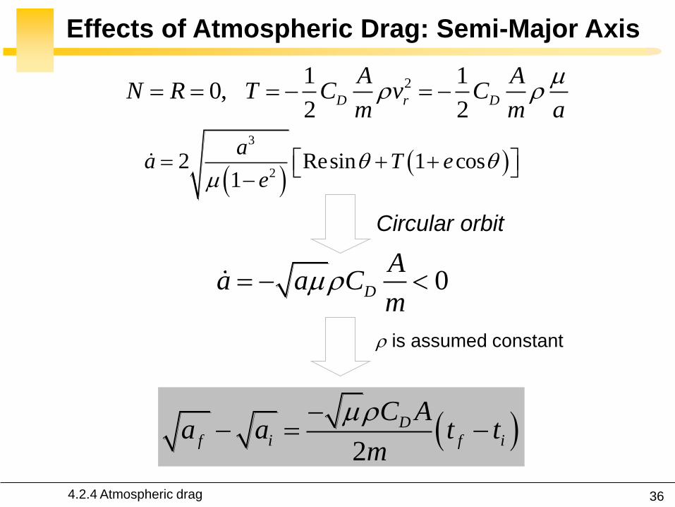
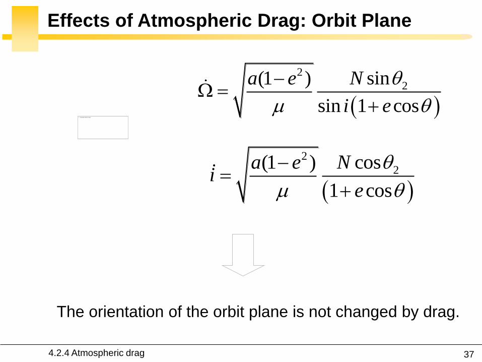
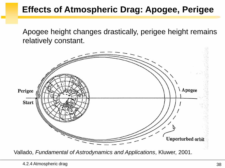
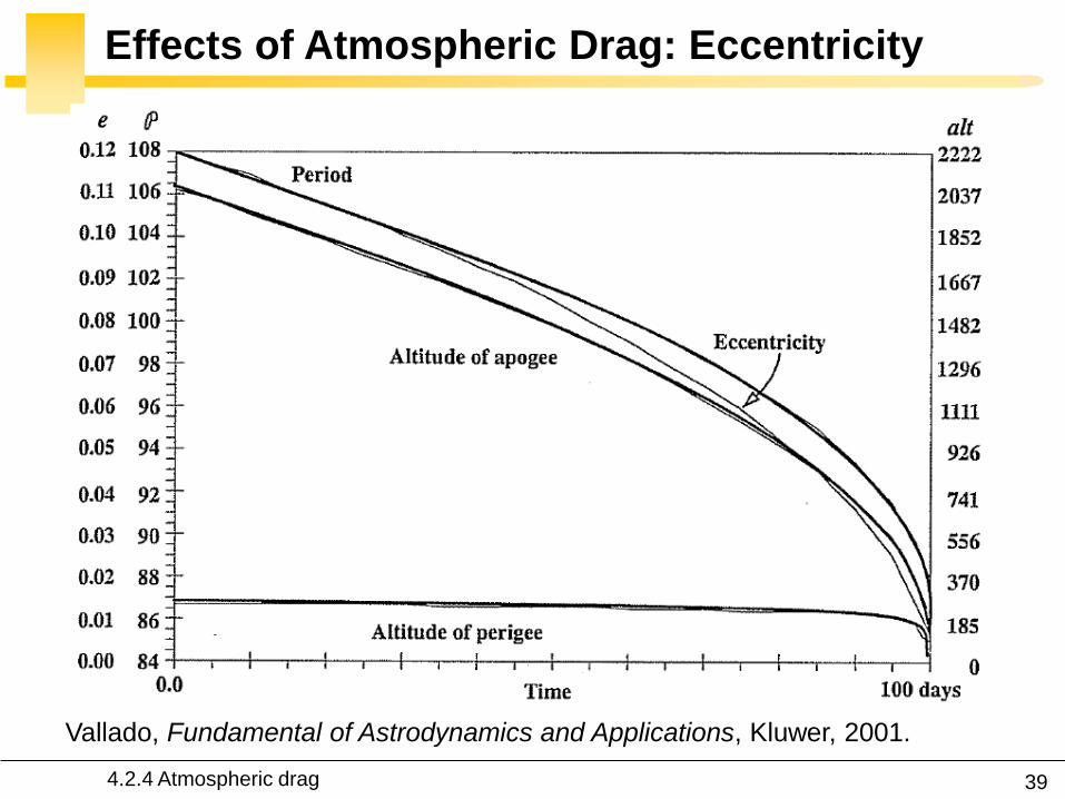
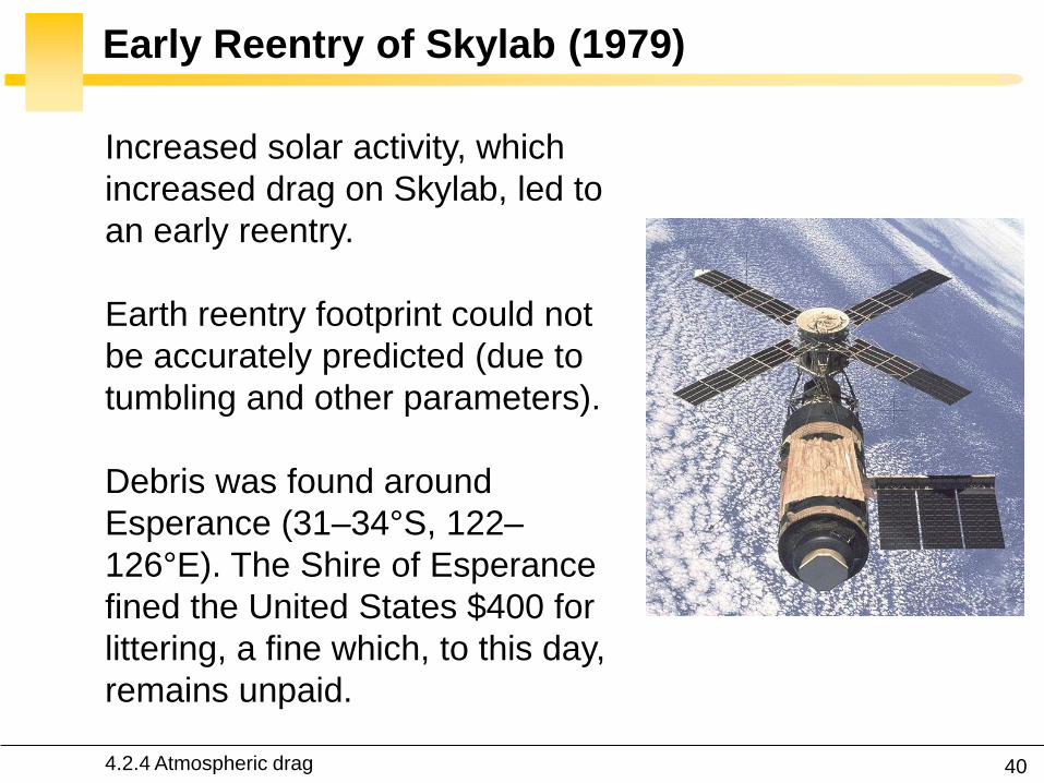
40
Early Reentry of Skylab (1979)
Increased solar activity which
increased drag on Skylab led to
an early reentry
Earth reentry footprint could not
be accurately predicted (due to
tumbling and other parameters)
Debris was found around
Esperance (31ndash34degS 122ndash
126degE) The Shire of Esperance
fined the United States $400 for
littering a fine which to this day
remains unpaid
424 Atmospheric drag
41
Lost of ASCA Satellite (2000)
July 15 2000 a strong solar
flare heated the Earthrsquos
atmosphere increasing the
air density to a value 100
times greater than that for
which its ADCS had been
designed to cope The
magnetorquers were unable
to compensate and the
satellite was lost
httpheasarcgsfcnasagovdocsascasafemodehtml
424 Atmospheric drag
42
Effects of Third-Body Perturbations
The only secular perturbations are in the node and in the
perigee
For near-Earth orbits the dominance of the oblateness
dictates that the orbital plane regresses about the polar
axis For higher orbits the regression will be about some
mean pole lying between the Earthrsquos pole and the ecliptic
pole
Many geosynchronous satellites launched 30 years ago
now have inclinations of up to plusmn15ordm collision avoidance
as the satellites drift back through the GEO belt
425 Third-body perturbations
43
Effects of Third-Body Perturbations
Vallado Fundamental of Astrodynamics and Applications Kluwer 2001
The Sunrsquos attraction
tends to turn the
satellite ring into the
ecliptic The orbit
precesses about the
pole of the ecliptic
425 Third-body perturbations
44
STK Analytic Propagator (SGP4)
The J2 propagator does not include drag
SGP4 which stands for Simplified General Perturbations
Satellite Orbit Model 4 is a NASANORAD algorithm
426 SGP4 propagator in STK
45
STK Analytic Propagator (SGP4)
Several assumptions propagation valid for short durations
(3-10 days)
TLE data should be used as the input (see Lecture 03)
It considers secular and periodic variations due to Earth
oblateness solar and lunar gravitational effects and
orbital decay using a drag model
426 SGP4 propagator in STK
46
SGP4 Applied to ISS RAAN
426 SGP4 propagator in STK
47
SGP4 Applied to ISS Semi-Major Axis
426 SGP4 propagator in STK
48
Further Reading on the Web Site
426 SGP4 propagator in STK
49
Effects of Solar Radiation Pressure
The effects are usually small for most satellites
Satellites with very low mass and large surface area are
more affected
427 Solar radiation pressure
Vallado Fundamental of
Astrodynamics and
Applications Kluwer
2001
51
Secular Effects Orders of Magnitude
Vallado Fundamental of Astrodynamics and Applications Kluwer 2001
52
Periodic Effects Orders of Magnitude
Vallado Fundamental of Astrodynamics and Applications Kluwer 2001
53
4 Non-Keplerian Motion
2
2
(1 )
sin
sin 1 cos
a e
N
i e
43 Numerical methods
431 Orbit prediction
432 Numerical integration
433 Single-step methods Runge-Kutta
434 Multi-step methods
435 Integrator and step size selection
436 ISS example
nt 1nt
r
54
2-body analytic propagator (constant orbital elements)
J2 analytic propagator (secular variations in the orbit
elements due to Earth oblateness
HPOP numerical integration of the equations of motion
(periodic and secular effects included)
STK Propagators
431 Orbit prediction
Accurate
Versatile
Errors accumulation
for long intervals
Computationally
intensive
55
Real-Life Example German Aerospace Agency
431 Orbit prediction
56
Real-Life Example German Aerospace Agency
57
Further Reading on the Web Site
431 Orbit prediction
58
Real-Life Example Envisat
httpnngesocesadeenvisat
ENVpredhtml
431 Orbit prediction
Why do the
predictions degrade
for lower altitudes
60
NASA began the first complex numerical integrations
during the late 1960s and early 1970s
Did you Know
1969 1968
431 Orbit prediction
61
What is Numerical Integration
1n nt t t
3 perturbedr
r r a
Given
Compute
( ) ( )n nt tr r
1 1( ) ( )n nt t r r
432 Numerical integration
62
State-Space Formulation
3 perturbedr
r r a
( )f tu u
ru
r
6-dimensional
state vector
432 Numerical integration
63
How to Perform Numerical Integration
2( )( ) ( ) ( ) ( ) ( )
2
ss
n n n n n s
h hf t h f t hf t f t f t R
s
Taylor series expansion
( )ntu
1( )nt u
432 Numerical integration
64
First-Order Taylor Approximation (Euler)
1
( ) ( ) ( )
( )
n n n
n n n n
t t t t t
t f t
u u u
u u uEuler step
0 1 2 3 4 5 60
5
10
15
20
25
30
35
40
Time t (s)
x(t
)=t2
Exact solution
The stepsize has to be extremely
small for accurate predictions
and it is necessary to develop
more effective algorithms
along the tangent
432 Numerical integration
65
Numerical Integration Methods
1 1 1
1 0
m m
n j n j j n j
j j
t
u u u
0 0
Implicit the solution method becomes
iterative in the nonlinear case
0 0 Explicit un+1 can be deduced directly from
the results at the previous time steps
=0
for 1
j j
j
Single-step the system at time tn+1
only depends on the previous state tn
State vector
0
for 1
j j
j
Multi-step the system at time tn+1 depends
several previous states tntn-1etc
432 Numerical integration
66
Examples Implicit vs Explicit
Trapezoidal rule (implicit)
nt 1nt
Euler forward (explicit)
nt 1nt
Euler backward (implicit)
nt 1nt
1n n nt u u u
1 1n n nt u u u
1
12
n n
n n t
u uu u
r
r
r
432 Numerical integration
67
A variety of methods has been applied in astrodynamics
Each of these methods has its own advantages and
drawbacks
Accuracy what is the order of the integration scheme
Efficiency how many function calls
Versatility can it be applied to a wide range of problems
Complexity is it easy to implement and use
Step size automatic step size control
Why Different Methods
431 Orbit prediction
68
Runge-Kutta Family Single-Step
Perhaps the most well-known numerical integrator
Difference with traditional Taylor series integrators the RK
family only requires the first derivative but several
evaluations are needed to move forward one step in time
Different variants explicit embedded etc
433 Single-step methods Runge-Kutta
69
Runge-Kutta Family Single-Step
with ( ) ( )t f tu u 0 0( )t u u
1
1
s
n n i i
i
t b
u u k
1 1
1
1
2
n n
i
i n ij j n i
j
f t c t
f t a t c t i s
k u
k u k
Slopes at
various points
within the
integration step
433 Single-step methods Runge-Kutta
70
Runge-Kutta Family Single-Step
Butcher Tableau
The Runge-Kutta methods are fully described by the
coefficients
c1
c2
cs
a21
as1
b1
as2
b2
ass-1
bs-1 hellip
hellip
hellip hellip hellip
bs
1
1
1
1
1
0
s
i
i
i
i ij
j
b
c
c a
433 Single-step methods Runge-Kutta
71
RK4 (Explicit)
1 2 3 41
2 2
6n n t
k k k ku u
Butcher Tableau
1
2 1
3 2
4 3
2 2
2 2
n n
n n
n n
n n
f t
t tf t
t tf t
f t t t
k u
k u k
k u k
k u k
433 Single-step methods Runge-Kutta
72
RK4 (Explicit)
1 2 3 41
2 2
6n n t
k k k ku u
1
2 1
3 2
4 3
2 2
2 2
n n
n n
n n
n n
f t
t tf t
t tf t
f t t t
k u
k u k
k u k
k u k
Slope at the beginning
Slope at the midpoint (k1 is
used to determine the value
of u Euler)
Slope at the midpoint (k2 is
now used)
Slope at the end
Estimated slope
(weighted average)
433 Single-step methods Runge-Kutta
73
RK4 (Explicit)
nt 2nt t nt t
1k3k
2k
4k
Estimate at new
time
u
433 Single-step methods Runge-Kutta
74
RK4 (Explicit)
The local truncation error for a 4th order RK is O(h5)
The accuracy is comparable to that of a 4th order Taylor
series but the Runge-Kutta method avoids the
calculation of higher-order derivatives
Easy to use and implement
The step size is fixed
433 Single-step methods Runge-Kutta
75
RK4 in STK
433 Single-step methods Runge-Kutta
76
Embedded Methods
They produce an estimate of the local truncation error
adjust the step size to keep local truncation errors
within some tolerances
This is done by having two methods in the tableau one with
order p and one with order p+1 with the same set of
function evaluations
( 1) ( 1) ( 1)
1
1
sp p p
n n i i
i
t b
u u k
( ) ( ) ( )
1
1
sp p p
n n i i
i
t b
u u k
433 Single-step methods Runge-Kutta
77
Embedded Methods
The two different approximations for the solution at each
step are compared
If the two answers are in close agreement the approximation is
accepted
If the two answers do not agree to a specified accuracy the step
size is reduced
If the answers agree to more significant digits than required the
step size is increased
433 Single-step methods Runge-Kutta
78
Ode45 in Matlab Simulink
Runge-Kutta (45) pair of Dormand and Prince
Variable step size
Matlab help This should be the first solver you try
433 Single-step methods Runge-Kutta
79
Ode45 in Matlab Simulink
edit ode45
433 Single-step methods Runge-Kutta
80
Ode45 in Matlab Simulink
Be very careful with the default parameters
options = odeset(RelTol1e-8AbsTol1e-8)
433 Single-step methods Runge-Kutta
81
RKF 7(8) Default Method in STK
Runge-Kutta-Fehlberg integration method of 7th order
with 8th order error control for the integration step size
433 Single-step methods Runge-Kutta
83
Multi-Step Methods (Predictor-Corrector)
They estimate the state over time using previously
determined back values of the solution
Unlike RK methods they only perform one evaluation for
each step forward but they usually have a predictor and a
corrector formula
Adams() ndash Bashforth - Moulton Gauss - Jackson
() The first with Le Verrier to predict the existence and position of Neptune
434 Multi-step methods
84
Multi-Step Methods Principle
( ) ( )t f tu u1
1( ) ( ) ( ) n
n
t
n nt
t t f t dt
u u u
unknown
Replace it by a
polynomial that
interpolates the
previous values Four function values
interpolated by a
third-order polynomial
t
u
434 Multi-step methods
85
Multi-Step Methods Initiation
with ( ) ( )t f tu u 0 0( )t u u
What is the inherent problem
t
u
434 Multi-step methods
86
Multi-Step Methods Initiation
Because these methods require back values they are not
self-starting
One may for instance use of a single-step method to
compute the first four values
434 Multi-step methods
87
Gauss-Jackson in STK
One of the most recommendable fixed-stepsize multistep
methods for orbit computations
88
Integrator Selection
435 Integrator and step size selection
Montenbruck and Gill
Satellite orbits Springer
2000
89
Integrator Selection
Pros
Very fast
Cons
Special starting procedure
Fixed time steps
Error control
Pros
Plug and play
Error control
Cons
Slower
Multi-step Single step
435 Integrator and step size selection
90
Why is the Step Size So Critical
Theoretical arguments
1 The accuracy and the stability of the algorithm are
directly related to the step size
2 Nonlinear equations of motion
Data for Landsat 4 and 6 in circular orbits around 800km
indicates that a one-minute step size yields about 47m
error
A three-minute step size produces about a 900m error
435 Integrator and step size selection
91
Why is the Step Size So Critical
More practical arguments
1 The computation time is directly related to the
step size
2 The particular choice of step size depends on the
most rapidly varying component in the disturbing
functions (eg 50 x 50 gravity field)
435 Integrator and step size selection
92
Appropriate Step Size
The problem of determining an appropriate step size is a
challenge in any numerical process
Fixed step size (rule of thumb for standard
applications)
But an algorithm with variable step size is really
helpful The step size is chosen in such a way that
each step contributes uniformly to the total integration
error
100
orbitTt
435 Integrator and step size selection
93
Three Examples XMM OUFTI-1 ISS
Can you plot the step size vs true anomaly
435 Integrator and step size selection
94
XMM Report in STK
435 Integrator and step size selection
95
XMM (e~08)
0 50 100 150 200 250 300 350 4000
1000
2000
3000
4000
5000
6000
True anomaly (deg)
Ste
p s
ize
(s)
435 Integrator and step size selection
96
ISS(e~0)
435 Integrator and step size selection
0 50 100 150 200 250 300 350 40030
35
40
45
50
55
60
65
70
True anomaly (deg)
Ste
p s
ize
(s)
97
ldquoDifficultrdquo Orbits
Automatic time step is especially nice on highly eccentric
orbits (Molniya XMM) These orbits are best computed
using variable step sizes to maintain some given level of
accuracy
Without this variable step size we waste a lot of time near
apoapsis when the integration is taking too small a step
Likewise the integrator may not be using a small enough step
size at periapsis where the satellite is traveling fast
435 Integrator and step size selection
98
HPOP Propagator ISS Example
1 Earthrsquos oblateness only
2 Drag only
3 Sun and moon only
4 SRP only
5 All together
436 ISS example
99
Earthrsquos Oblateness Only Ω
HPOP
J2
2-body
436 ISS example
100
Earthrsquos Oblateness Only i Ω a
HPOP with central body (20 + WGS84_EGM96)
(without dragSRPSun and Moon)
436 ISS example
101
Drag Only i Ω a
HPOP with drag ndash Harris Priester
(without oblatenessSRPSun and Moon)
436 ISS example
102
Drag Relationship with Eclipses
103
SRP Only i Ω a
HPOP with SRP
(without oblatenessdragSun and Moon)
436 ISS example
104
SRP Relationship with Eclipses
105
All Perturbations Together
436 ISS example
106
4 Non-Keplerian Motion
2
2
(1 )
sin
sin 1 cos
a e
N
i e
44 Geostationary satellites
107
Practical Example GEO Satellites
Nice illustration of
1 Perturbations of the 2-body problem
2 Secular and periodic contributions
3 Accuracy required by practical applications
4 The need for orbit correction and thrust forces
And it is a real-life example (telecommunications
meteorology)
44 GEO satellites
108
Three Main Perturbations for GEO Satellites
44 GEO satellites
1 Non-spherical Earth
2 SRP
3 Sun and Moon
109
Station Keeping of GEO Satellites
The effect of the perturbations is to cause the spacecraft
to drift away from its nominal station If the drift was
allowed to build up unchecked the spacecraft could
become useless
A station-keeping box is defined by a longitude and a
maximum authorized distance for satellite excursions in
longitude and latitude
For instance TC2 -8ordm plusmn 007ordm EW plusmn 005ordm NS
44 GEO satellites
110
East-West and North-South Drift
44 GEO satellites
NS drift
EW drift
What are the perturbations generating these drifts
111
East-West Drift
44 GEO satellites
A GEO satellite drifts in longitude due to the influence of
two main perturbations
1 The elliptic nature of the Earthrsquos equatorial cross-
section J22 (and not from the NS oblateness J2)
2
ΔV
ΔV vsat
vsat SRP
112
East-West Drift due to Equatorial Ellipticity
44 GEO satellites
113
East-West Drift due to Equatorial Ellipticity
44 GEO satellites
114
East-West Drift HPOP (20) vs HPOP (22)
44 GEO satellites
115
East-West Drift Stable Equilibirum
HPOP with 22
(without Sun and moonSRPdrag)
116
East-West Drift Stable Equilibirum
HPOP with 22
(without Sun and moonSRPdrag)
117
East-West Drift Stable Equilibirum
HPOP with 22
(without Sun and moonSRPdrag)
118
North-South Drift
The perturbations caused by the Sun and the Moon are
predominantly out-of-plane effects causing a change in
the inclination and in the right ascension of the orbit
ascending node
Similar effects on the orbit to those of the Earthrsquos
oblateness (but here with respect to the ecliptic)
A GEO satellite therefore drifts in latitude with a
fundamental period equal to the orbit period
119
North-South Drift
Period
HPOP with Sun and Moon
(without oblatenessSRPdrag)
120
North-South Drift
Period
HPOP with Sun and Moon
(without oblatenessSRPdrag)
121
Thrust Forces for Stationkeeping
GEO spacecraft require continual stationkeeping to stay
within the authorized box using onboard thrusters
44 GEO satellites
122
42 ANALYTIC TREATMENT
421 Variation of parameters
422 Non-spherical Earth
423 J2 propagator in STK
424 Atmospheric drag
425 Third-body perturbations
426 SGP4 propagator in STK
427 Solar radiation pressure
4 Non-Keplerian Motion
43 NUMERICAL METHODS
431 Orbit prediction
432 Numerical integration
433 Single-step methods Runge-Kutta
434 Multi-step methods
435 Integrator and step size selection
436 ISS example
44 GEOSTATIONARY SATELLITES
Gaeumltan Kerschen
Space Structures amp
Systems Lab (S3L)
4B Non-Keplerian Motion
Astrodynamics (AERO0024)
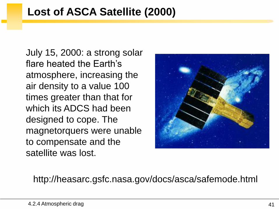
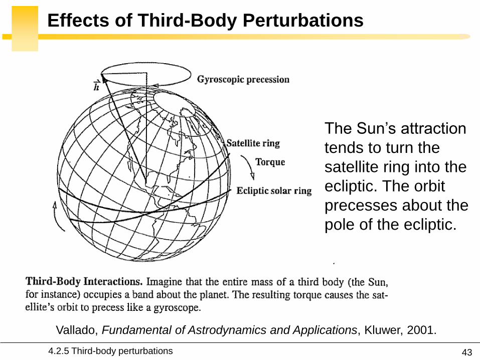
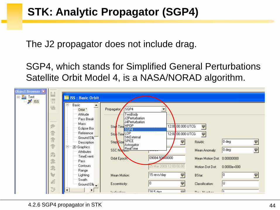
45
STK Analytic Propagator (SGP4)
Several assumptions propagation valid for short durations
(3-10 days)
TLE data should be used as the input (see Lecture 03)
It considers secular and periodic variations due to Earth
oblateness solar and lunar gravitational effects and
orbital decay using a drag model
426 SGP4 propagator in STK
46
SGP4 Applied to ISS RAAN
426 SGP4 propagator in STK
47
SGP4 Applied to ISS Semi-Major Axis
426 SGP4 propagator in STK
48
Further Reading on the Web Site
426 SGP4 propagator in STK
49
Effects of Solar Radiation Pressure
The effects are usually small for most satellites
Satellites with very low mass and large surface area are
more affected
427 Solar radiation pressure
Vallado Fundamental of
Astrodynamics and
Applications Kluwer
2001
51
Secular Effects Orders of Magnitude
Vallado Fundamental of Astrodynamics and Applications Kluwer 2001
52
Periodic Effects Orders of Magnitude
Vallado Fundamental of Astrodynamics and Applications Kluwer 2001
53
4 Non-Keplerian Motion
2
2
(1 )
sin
sin 1 cos
a e
N
i e
43 Numerical methods
431 Orbit prediction
432 Numerical integration
433 Single-step methods Runge-Kutta
434 Multi-step methods
435 Integrator and step size selection
436 ISS example
nt 1nt
r
54
2-body analytic propagator (constant orbital elements)
J2 analytic propagator (secular variations in the orbit
elements due to Earth oblateness
HPOP numerical integration of the equations of motion
(periodic and secular effects included)
STK Propagators
431 Orbit prediction
Accurate
Versatile
Errors accumulation
for long intervals
Computationally
intensive
55
Real-Life Example German Aerospace Agency
431 Orbit prediction
56
Real-Life Example German Aerospace Agency
57
Further Reading on the Web Site
431 Orbit prediction
58
Real-Life Example Envisat
httpnngesocesadeenvisat
ENVpredhtml
431 Orbit prediction
Why do the
predictions degrade
for lower altitudes
60
NASA began the first complex numerical integrations
during the late 1960s and early 1970s
Did you Know
1969 1968
431 Orbit prediction
61
What is Numerical Integration
1n nt t t
3 perturbedr
r r a
Given
Compute
( ) ( )n nt tr r
1 1( ) ( )n nt t r r
432 Numerical integration
62
State-Space Formulation
3 perturbedr
r r a
( )f tu u
ru
r
6-dimensional
state vector
432 Numerical integration
63
How to Perform Numerical Integration
2( )( ) ( ) ( ) ( ) ( )
2
ss
n n n n n s
h hf t h f t hf t f t f t R
s
Taylor series expansion
( )ntu
1( )nt u
432 Numerical integration
64
First-Order Taylor Approximation (Euler)
1
( ) ( ) ( )
( )
n n n
n n n n
t t t t t
t f t
u u u
u u uEuler step
0 1 2 3 4 5 60
5
10
15
20
25
30
35
40
Time t (s)
x(t
)=t2
Exact solution
The stepsize has to be extremely
small for accurate predictions
and it is necessary to develop
more effective algorithms
along the tangent
432 Numerical integration
65
Numerical Integration Methods
1 1 1
1 0
m m
n j n j j n j
j j
t
u u u
0 0
Implicit the solution method becomes
iterative in the nonlinear case
0 0 Explicit un+1 can be deduced directly from
the results at the previous time steps
=0
for 1
j j
j
Single-step the system at time tn+1
only depends on the previous state tn
State vector
0
for 1
j j
j
Multi-step the system at time tn+1 depends
several previous states tntn-1etc
432 Numerical integration
66
Examples Implicit vs Explicit
Trapezoidal rule (implicit)
nt 1nt
Euler forward (explicit)
nt 1nt
Euler backward (implicit)
nt 1nt
1n n nt u u u
1 1n n nt u u u
1
12
n n
n n t
u uu u
r
r
r
432 Numerical integration
67
A variety of methods has been applied in astrodynamics
Each of these methods has its own advantages and
drawbacks
Accuracy what is the order of the integration scheme
Efficiency how many function calls
Versatility can it be applied to a wide range of problems
Complexity is it easy to implement and use
Step size automatic step size control
Why Different Methods
431 Orbit prediction
68
Runge-Kutta Family Single-Step
Perhaps the most well-known numerical integrator
Difference with traditional Taylor series integrators the RK
family only requires the first derivative but several
evaluations are needed to move forward one step in time
Different variants explicit embedded etc
433 Single-step methods Runge-Kutta
69
Runge-Kutta Family Single-Step
with ( ) ( )t f tu u 0 0( )t u u
1
1
s
n n i i
i
t b
u u k
1 1
1
1
2
n n
i
i n ij j n i
j
f t c t
f t a t c t i s
k u
k u k
Slopes at
various points
within the
integration step
433 Single-step methods Runge-Kutta
70
Runge-Kutta Family Single-Step
Butcher Tableau
The Runge-Kutta methods are fully described by the
coefficients
c1
c2
cs
a21
as1
b1
as2
b2
ass-1
bs-1 hellip
hellip
hellip hellip hellip
bs
1
1
1
1
1
0
s
i
i
i
i ij
j
b
c
c a
433 Single-step methods Runge-Kutta
71
RK4 (Explicit)
1 2 3 41
2 2
6n n t
k k k ku u
Butcher Tableau
1
2 1
3 2
4 3
2 2
2 2
n n
n n
n n
n n
f t
t tf t
t tf t
f t t t
k u
k u k
k u k
k u k
433 Single-step methods Runge-Kutta
72
RK4 (Explicit)
1 2 3 41
2 2
6n n t
k k k ku u
1
2 1
3 2
4 3
2 2
2 2
n n
n n
n n
n n
f t
t tf t
t tf t
f t t t
k u
k u k
k u k
k u k
Slope at the beginning
Slope at the midpoint (k1 is
used to determine the value
of u Euler)
Slope at the midpoint (k2 is
now used)
Slope at the end
Estimated slope
(weighted average)
433 Single-step methods Runge-Kutta
73
RK4 (Explicit)
nt 2nt t nt t
1k3k
2k
4k
Estimate at new
time
u
433 Single-step methods Runge-Kutta
74
RK4 (Explicit)
The local truncation error for a 4th order RK is O(h5)
The accuracy is comparable to that of a 4th order Taylor
series but the Runge-Kutta method avoids the
calculation of higher-order derivatives
Easy to use and implement
The step size is fixed
433 Single-step methods Runge-Kutta
75
RK4 in STK
433 Single-step methods Runge-Kutta
76
Embedded Methods
They produce an estimate of the local truncation error
adjust the step size to keep local truncation errors
within some tolerances
This is done by having two methods in the tableau one with
order p and one with order p+1 with the same set of
function evaluations
( 1) ( 1) ( 1)
1
1
sp p p
n n i i
i
t b
u u k
( ) ( ) ( )
1
1
sp p p
n n i i
i
t b
u u k
433 Single-step methods Runge-Kutta
77
Embedded Methods
The two different approximations for the solution at each
step are compared
If the two answers are in close agreement the approximation is
accepted
If the two answers do not agree to a specified accuracy the step
size is reduced
If the answers agree to more significant digits than required the
step size is increased
433 Single-step methods Runge-Kutta
78
Ode45 in Matlab Simulink
Runge-Kutta (45) pair of Dormand and Prince
Variable step size
Matlab help This should be the first solver you try
433 Single-step methods Runge-Kutta
79
Ode45 in Matlab Simulink
edit ode45
433 Single-step methods Runge-Kutta
80
Ode45 in Matlab Simulink
Be very careful with the default parameters
options = odeset(RelTol1e-8AbsTol1e-8)
433 Single-step methods Runge-Kutta
81
RKF 7(8) Default Method in STK
Runge-Kutta-Fehlberg integration method of 7th order
with 8th order error control for the integration step size
433 Single-step methods Runge-Kutta
83
Multi-Step Methods (Predictor-Corrector)
They estimate the state over time using previously
determined back values of the solution
Unlike RK methods they only perform one evaluation for
each step forward but they usually have a predictor and a
corrector formula
Adams() ndash Bashforth - Moulton Gauss - Jackson
() The first with Le Verrier to predict the existence and position of Neptune
434 Multi-step methods
84
Multi-Step Methods Principle
( ) ( )t f tu u1
1( ) ( ) ( ) n
n
t
n nt
t t f t dt
u u u
unknown
Replace it by a
polynomial that
interpolates the
previous values Four function values
interpolated by a
third-order polynomial
t
u
434 Multi-step methods
85
Multi-Step Methods Initiation
with ( ) ( )t f tu u 0 0( )t u u
What is the inherent problem
t
u
434 Multi-step methods
86
Multi-Step Methods Initiation
Because these methods require back values they are not
self-starting
One may for instance use of a single-step method to
compute the first four values
434 Multi-step methods
87
Gauss-Jackson in STK
One of the most recommendable fixed-stepsize multistep
methods for orbit computations
88
Integrator Selection
435 Integrator and step size selection
Montenbruck and Gill
Satellite orbits Springer
2000
89
Integrator Selection
Pros
Very fast
Cons
Special starting procedure
Fixed time steps
Error control
Pros
Plug and play
Error control
Cons
Slower
Multi-step Single step
435 Integrator and step size selection
90
Why is the Step Size So Critical
Theoretical arguments
1 The accuracy and the stability of the algorithm are
directly related to the step size
2 Nonlinear equations of motion
Data for Landsat 4 and 6 in circular orbits around 800km
indicates that a one-minute step size yields about 47m
error
A three-minute step size produces about a 900m error
435 Integrator and step size selection
91
Why is the Step Size So Critical
More practical arguments
1 The computation time is directly related to the
step size
2 The particular choice of step size depends on the
most rapidly varying component in the disturbing
functions (eg 50 x 50 gravity field)
435 Integrator and step size selection
92
Appropriate Step Size
The problem of determining an appropriate step size is a
challenge in any numerical process
Fixed step size (rule of thumb for standard
applications)
But an algorithm with variable step size is really
helpful The step size is chosen in such a way that
each step contributes uniformly to the total integration
error
100
orbitTt
435 Integrator and step size selection
93
Three Examples XMM OUFTI-1 ISS
Can you plot the step size vs true anomaly
435 Integrator and step size selection
94
XMM Report in STK
435 Integrator and step size selection
95
XMM (e~08)
0 50 100 150 200 250 300 350 4000
1000
2000
3000
4000
5000
6000
True anomaly (deg)
Ste
p s
ize
(s)
435 Integrator and step size selection
96
ISS(e~0)
435 Integrator and step size selection
0 50 100 150 200 250 300 350 40030
35
40
45
50
55
60
65
70
True anomaly (deg)
Ste
p s
ize
(s)
97
ldquoDifficultrdquo Orbits
Automatic time step is especially nice on highly eccentric
orbits (Molniya XMM) These orbits are best computed
using variable step sizes to maintain some given level of
accuracy
Without this variable step size we waste a lot of time near
apoapsis when the integration is taking too small a step
Likewise the integrator may not be using a small enough step
size at periapsis where the satellite is traveling fast
435 Integrator and step size selection
98
HPOP Propagator ISS Example
1 Earthrsquos oblateness only
2 Drag only
3 Sun and moon only
4 SRP only
5 All together
436 ISS example
99
Earthrsquos Oblateness Only Ω
HPOP
J2
2-body
436 ISS example
100
Earthrsquos Oblateness Only i Ω a
HPOP with central body (20 + WGS84_EGM96)
(without dragSRPSun and Moon)
436 ISS example
101
Drag Only i Ω a
HPOP with drag ndash Harris Priester
(without oblatenessSRPSun and Moon)
436 ISS example
102
Drag Relationship with Eclipses
103
SRP Only i Ω a
HPOP with SRP
(without oblatenessdragSun and Moon)
436 ISS example
104
SRP Relationship with Eclipses
105
All Perturbations Together
436 ISS example
106
4 Non-Keplerian Motion
2
2
(1 )
sin
sin 1 cos
a e
N
i e
44 Geostationary satellites
107
Practical Example GEO Satellites
Nice illustration of
1 Perturbations of the 2-body problem
2 Secular and periodic contributions
3 Accuracy required by practical applications
4 The need for orbit correction and thrust forces
And it is a real-life example (telecommunications
meteorology)
44 GEO satellites
108
Three Main Perturbations for GEO Satellites
44 GEO satellites
1 Non-spherical Earth
2 SRP
3 Sun and Moon
109
Station Keeping of GEO Satellites
The effect of the perturbations is to cause the spacecraft
to drift away from its nominal station If the drift was
allowed to build up unchecked the spacecraft could
become useless
A station-keeping box is defined by a longitude and a
maximum authorized distance for satellite excursions in
longitude and latitude
For instance TC2 -8ordm plusmn 007ordm EW plusmn 005ordm NS
44 GEO satellites
110
East-West and North-South Drift
44 GEO satellites
NS drift
EW drift
What are the perturbations generating these drifts
111
East-West Drift
44 GEO satellites
A GEO satellite drifts in longitude due to the influence of
two main perturbations
1 The elliptic nature of the Earthrsquos equatorial cross-
section J22 (and not from the NS oblateness J2)
2
ΔV
ΔV vsat
vsat SRP
112
East-West Drift due to Equatorial Ellipticity
44 GEO satellites
113
East-West Drift due to Equatorial Ellipticity
44 GEO satellites
114
East-West Drift HPOP (20) vs HPOP (22)
44 GEO satellites
115
East-West Drift Stable Equilibirum
HPOP with 22
(without Sun and moonSRPdrag)
116
East-West Drift Stable Equilibirum
HPOP with 22
(without Sun and moonSRPdrag)
117
East-West Drift Stable Equilibirum
HPOP with 22
(without Sun and moonSRPdrag)
118
North-South Drift
The perturbations caused by the Sun and the Moon are
predominantly out-of-plane effects causing a change in
the inclination and in the right ascension of the orbit
ascending node
Similar effects on the orbit to those of the Earthrsquos
oblateness (but here with respect to the ecliptic)
A GEO satellite therefore drifts in latitude with a
fundamental period equal to the orbit period
119
North-South Drift
Period
HPOP with Sun and Moon
(without oblatenessSRPdrag)
120
North-South Drift
Period
HPOP with Sun and Moon
(without oblatenessSRPdrag)
121
Thrust Forces for Stationkeeping
GEO spacecraft require continual stationkeeping to stay
within the authorized box using onboard thrusters
44 GEO satellites
122
42 ANALYTIC TREATMENT
421 Variation of parameters
422 Non-spherical Earth
423 J2 propagator in STK
424 Atmospheric drag
425 Third-body perturbations
426 SGP4 propagator in STK
427 Solar radiation pressure
4 Non-Keplerian Motion
43 NUMERICAL METHODS
431 Orbit prediction
432 Numerical integration
433 Single-step methods Runge-Kutta
434 Multi-step methods
435 Integrator and step size selection
436 ISS example
44 GEOSTATIONARY SATELLITES
Gaeumltan Kerschen
Space Structures amp
Systems Lab (S3L)
4B Non-Keplerian Motion
Astrodynamics (AERO0024)
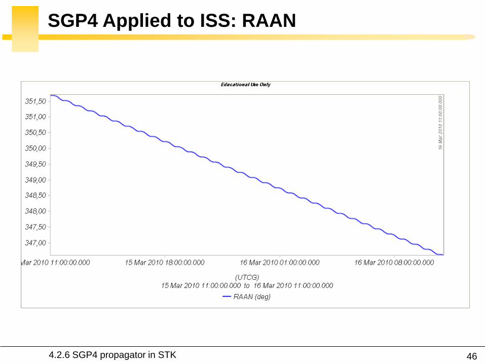
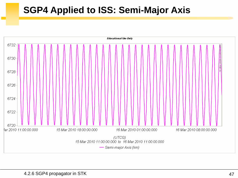
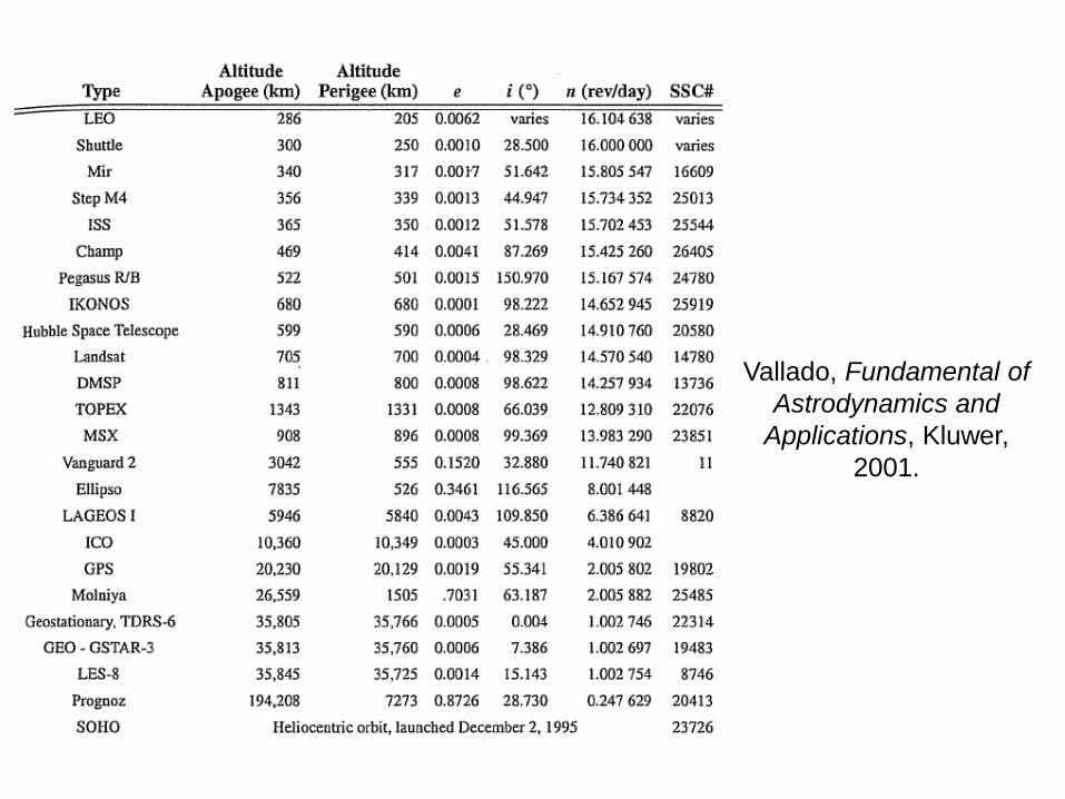
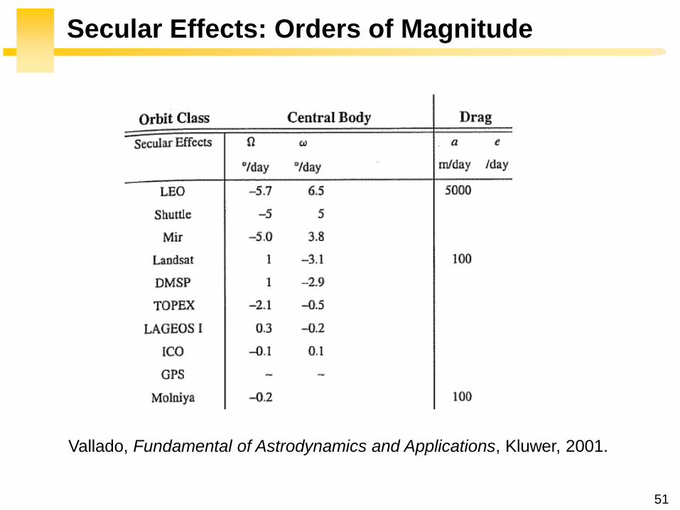
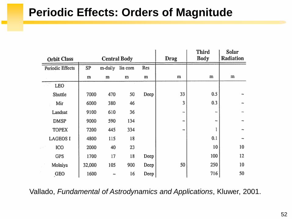
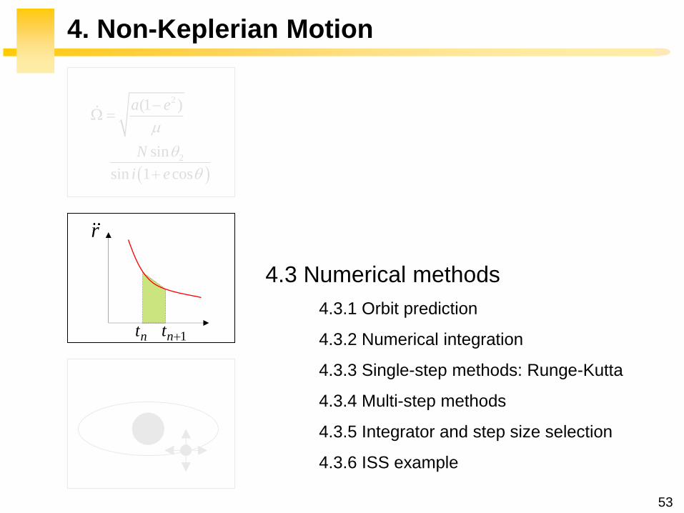
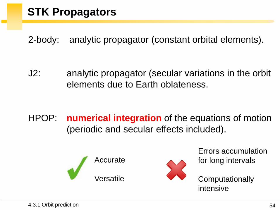
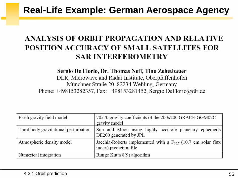
55
Real-Life Example German Aerospace Agency
431 Orbit prediction
56
Real-Life Example German Aerospace Agency
57
Further Reading on the Web Site
431 Orbit prediction
58
Real-Life Example Envisat
httpnngesocesadeenvisat
ENVpredhtml
431 Orbit prediction
Why do the
predictions degrade
for lower altitudes
60
NASA began the first complex numerical integrations
during the late 1960s and early 1970s
Did you Know
1969 1968
431 Orbit prediction
61
What is Numerical Integration
1n nt t t
3 perturbedr
r r a
Given
Compute
( ) ( )n nt tr r
1 1( ) ( )n nt t r r
432 Numerical integration
62
State-Space Formulation
3 perturbedr
r r a
( )f tu u
ru
r
6-dimensional
state vector
432 Numerical integration
63
How to Perform Numerical Integration
2( )( ) ( ) ( ) ( ) ( )
2
ss
n n n n n s
h hf t h f t hf t f t f t R
s
Taylor series expansion
( )ntu
1( )nt u
432 Numerical integration
64
First-Order Taylor Approximation (Euler)
1
( ) ( ) ( )
( )
n n n
n n n n
t t t t t
t f t
u u u
u u uEuler step
0 1 2 3 4 5 60
5
10
15
20
25
30
35
40
Time t (s)
x(t
)=t2
Exact solution
The stepsize has to be extremely
small for accurate predictions
and it is necessary to develop
more effective algorithms
along the tangent
432 Numerical integration
65
Numerical Integration Methods
1 1 1
1 0
m m
n j n j j n j
j j
t
u u u
0 0
Implicit the solution method becomes
iterative in the nonlinear case
0 0 Explicit un+1 can be deduced directly from
the results at the previous time steps
=0
for 1
j j
j
Single-step the system at time tn+1
only depends on the previous state tn
State vector
0
for 1
j j
j
Multi-step the system at time tn+1 depends
several previous states tntn-1etc
432 Numerical integration
66
Examples Implicit vs Explicit
Trapezoidal rule (implicit)
nt 1nt
Euler forward (explicit)
nt 1nt
Euler backward (implicit)
nt 1nt
1n n nt u u u
1 1n n nt u u u
1
12
n n
n n t
u uu u
r
r
r
432 Numerical integration
67
A variety of methods has been applied in astrodynamics
Each of these methods has its own advantages and
drawbacks
Accuracy what is the order of the integration scheme
Efficiency how many function calls
Versatility can it be applied to a wide range of problems
Complexity is it easy to implement and use
Step size automatic step size control
Why Different Methods
431 Orbit prediction
68
Runge-Kutta Family Single-Step
Perhaps the most well-known numerical integrator
Difference with traditional Taylor series integrators the RK
family only requires the first derivative but several
evaluations are needed to move forward one step in time
Different variants explicit embedded etc
433 Single-step methods Runge-Kutta
69
Runge-Kutta Family Single-Step
with ( ) ( )t f tu u 0 0( )t u u
1
1
s
n n i i
i
t b
u u k
1 1
1
1
2
n n
i
i n ij j n i
j
f t c t
f t a t c t i s
k u
k u k
Slopes at
various points
within the
integration step
433 Single-step methods Runge-Kutta
70
Runge-Kutta Family Single-Step
Butcher Tableau
The Runge-Kutta methods are fully described by the
coefficients
c1
c2
cs
a21
as1
b1
as2
b2
ass-1
bs-1 hellip
hellip
hellip hellip hellip
bs
1
1
1
1
1
0
s
i
i
i
i ij
j
b
c
c a
433 Single-step methods Runge-Kutta
71
RK4 (Explicit)
1 2 3 41
2 2
6n n t
k k k ku u
Butcher Tableau
1
2 1
3 2
4 3
2 2
2 2
n n
n n
n n
n n
f t
t tf t
t tf t
f t t t
k u
k u k
k u k
k u k
433 Single-step methods Runge-Kutta
72
RK4 (Explicit)
1 2 3 41
2 2
6n n t
k k k ku u
1
2 1
3 2
4 3
2 2
2 2
n n
n n
n n
n n
f t
t tf t
t tf t
f t t t
k u
k u k
k u k
k u k
Slope at the beginning
Slope at the midpoint (k1 is
used to determine the value
of u Euler)
Slope at the midpoint (k2 is
now used)
Slope at the end
Estimated slope
(weighted average)
433 Single-step methods Runge-Kutta
73
RK4 (Explicit)
nt 2nt t nt t
1k3k
2k
4k
Estimate at new
time
u
433 Single-step methods Runge-Kutta
74
RK4 (Explicit)
The local truncation error for a 4th order RK is O(h5)
The accuracy is comparable to that of a 4th order Taylor
series but the Runge-Kutta method avoids the
calculation of higher-order derivatives
Easy to use and implement
The step size is fixed
433 Single-step methods Runge-Kutta
75
RK4 in STK
433 Single-step methods Runge-Kutta
76
Embedded Methods
They produce an estimate of the local truncation error
adjust the step size to keep local truncation errors
within some tolerances
This is done by having two methods in the tableau one with
order p and one with order p+1 with the same set of
function evaluations
( 1) ( 1) ( 1)
1
1
sp p p
n n i i
i
t b
u u k
( ) ( ) ( )
1
1
sp p p
n n i i
i
t b
u u k
433 Single-step methods Runge-Kutta
77
Embedded Methods
The two different approximations for the solution at each
step are compared
If the two answers are in close agreement the approximation is
accepted
If the two answers do not agree to a specified accuracy the step
size is reduced
If the answers agree to more significant digits than required the
step size is increased
433 Single-step methods Runge-Kutta
78
Ode45 in Matlab Simulink
Runge-Kutta (45) pair of Dormand and Prince
Variable step size
Matlab help This should be the first solver you try
433 Single-step methods Runge-Kutta
79
Ode45 in Matlab Simulink
edit ode45
433 Single-step methods Runge-Kutta
80
Ode45 in Matlab Simulink
Be very careful with the default parameters
options = odeset(RelTol1e-8AbsTol1e-8)
433 Single-step methods Runge-Kutta
81
RKF 7(8) Default Method in STK
Runge-Kutta-Fehlberg integration method of 7th order
with 8th order error control for the integration step size
433 Single-step methods Runge-Kutta
83
Multi-Step Methods (Predictor-Corrector)
They estimate the state over time using previously
determined back values of the solution
Unlike RK methods they only perform one evaluation for
each step forward but they usually have a predictor and a
corrector formula
Adams() ndash Bashforth - Moulton Gauss - Jackson
() The first with Le Verrier to predict the existence and position of Neptune
434 Multi-step methods
84
Multi-Step Methods Principle
( ) ( )t f tu u1
1( ) ( ) ( ) n
n
t
n nt
t t f t dt
u u u
unknown
Replace it by a
polynomial that
interpolates the
previous values Four function values
interpolated by a
third-order polynomial
t
u
434 Multi-step methods
85
Multi-Step Methods Initiation
with ( ) ( )t f tu u 0 0( )t u u
What is the inherent problem
t
u
434 Multi-step methods
86
Multi-Step Methods Initiation
Because these methods require back values they are not
self-starting
One may for instance use of a single-step method to
compute the first four values
434 Multi-step methods
87
Gauss-Jackson in STK
One of the most recommendable fixed-stepsize multistep
methods for orbit computations
88
Integrator Selection
435 Integrator and step size selection
Montenbruck and Gill
Satellite orbits Springer
2000
89
Integrator Selection
Pros
Very fast
Cons
Special starting procedure
Fixed time steps
Error control
Pros
Plug and play
Error control
Cons
Slower
Multi-step Single step
435 Integrator and step size selection
90
Why is the Step Size So Critical
Theoretical arguments
1 The accuracy and the stability of the algorithm are
directly related to the step size
2 Nonlinear equations of motion
Data for Landsat 4 and 6 in circular orbits around 800km
indicates that a one-minute step size yields about 47m
error
A three-minute step size produces about a 900m error
435 Integrator and step size selection
91
Why is the Step Size So Critical
More practical arguments
1 The computation time is directly related to the
step size
2 The particular choice of step size depends on the
most rapidly varying component in the disturbing
functions (eg 50 x 50 gravity field)
435 Integrator and step size selection
92
Appropriate Step Size
The problem of determining an appropriate step size is a
challenge in any numerical process
Fixed step size (rule of thumb for standard
applications)
But an algorithm with variable step size is really
helpful The step size is chosen in such a way that
each step contributes uniformly to the total integration
error
100
orbitTt
435 Integrator and step size selection
93
Three Examples XMM OUFTI-1 ISS
Can you plot the step size vs true anomaly
435 Integrator and step size selection
94
XMM Report in STK
435 Integrator and step size selection
95
XMM (e~08)
0 50 100 150 200 250 300 350 4000
1000
2000
3000
4000
5000
6000
True anomaly (deg)
Ste
p s
ize
(s)
435 Integrator and step size selection
96
ISS(e~0)
435 Integrator and step size selection
0 50 100 150 200 250 300 350 40030
35
40
45
50
55
60
65
70
True anomaly (deg)
Ste
p s
ize
(s)
97
ldquoDifficultrdquo Orbits
Automatic time step is especially nice on highly eccentric
orbits (Molniya XMM) These orbits are best computed
using variable step sizes to maintain some given level of
accuracy
Without this variable step size we waste a lot of time near
apoapsis when the integration is taking too small a step
Likewise the integrator may not be using a small enough step
size at periapsis where the satellite is traveling fast
435 Integrator and step size selection
98
HPOP Propagator ISS Example
1 Earthrsquos oblateness only
2 Drag only
3 Sun and moon only
4 SRP only
5 All together
436 ISS example
99
Earthrsquos Oblateness Only Ω
HPOP
J2
2-body
436 ISS example
100
Earthrsquos Oblateness Only i Ω a
HPOP with central body (20 + WGS84_EGM96)
(without dragSRPSun and Moon)
436 ISS example
101
Drag Only i Ω a
HPOP with drag ndash Harris Priester
(without oblatenessSRPSun and Moon)
436 ISS example
102
Drag Relationship with Eclipses
103
SRP Only i Ω a
HPOP with SRP
(without oblatenessdragSun and Moon)
436 ISS example
104
SRP Relationship with Eclipses
105
All Perturbations Together
436 ISS example
106
4 Non-Keplerian Motion
2
2
(1 )
sin
sin 1 cos
a e
N
i e
44 Geostationary satellites
107
Practical Example GEO Satellites
Nice illustration of
1 Perturbations of the 2-body problem
2 Secular and periodic contributions
3 Accuracy required by practical applications
4 The need for orbit correction and thrust forces
And it is a real-life example (telecommunications
meteorology)
44 GEO satellites
108
Three Main Perturbations for GEO Satellites
44 GEO satellites
1 Non-spherical Earth
2 SRP
3 Sun and Moon
109
Station Keeping of GEO Satellites
The effect of the perturbations is to cause the spacecraft
to drift away from its nominal station If the drift was
allowed to build up unchecked the spacecraft could
become useless
A station-keeping box is defined by a longitude and a
maximum authorized distance for satellite excursions in
longitude and latitude
For instance TC2 -8ordm plusmn 007ordm EW plusmn 005ordm NS
44 GEO satellites
110
East-West and North-South Drift
44 GEO satellites
NS drift
EW drift
What are the perturbations generating these drifts
111
East-West Drift
44 GEO satellites
A GEO satellite drifts in longitude due to the influence of
two main perturbations
1 The elliptic nature of the Earthrsquos equatorial cross-
section J22 (and not from the NS oblateness J2)
2
ΔV
ΔV vsat
vsat SRP
112
East-West Drift due to Equatorial Ellipticity
44 GEO satellites
113
East-West Drift due to Equatorial Ellipticity
44 GEO satellites
114
East-West Drift HPOP (20) vs HPOP (22)
44 GEO satellites
115
East-West Drift Stable Equilibirum
HPOP with 22
(without Sun and moonSRPdrag)
116
East-West Drift Stable Equilibirum
HPOP with 22
(without Sun and moonSRPdrag)
117
East-West Drift Stable Equilibirum
HPOP with 22
(without Sun and moonSRPdrag)
118
North-South Drift
The perturbations caused by the Sun and the Moon are
predominantly out-of-plane effects causing a change in
the inclination and in the right ascension of the orbit
ascending node
Similar effects on the orbit to those of the Earthrsquos
oblateness (but here with respect to the ecliptic)
A GEO satellite therefore drifts in latitude with a
fundamental period equal to the orbit period
119
North-South Drift
Period
HPOP with Sun and Moon
(without oblatenessSRPdrag)
120
North-South Drift
Period
HPOP with Sun and Moon
(without oblatenessSRPdrag)
121
Thrust Forces for Stationkeeping
GEO spacecraft require continual stationkeeping to stay
within the authorized box using onboard thrusters
44 GEO satellites
122
42 ANALYTIC TREATMENT
421 Variation of parameters
422 Non-spherical Earth
423 J2 propagator in STK
424 Atmospheric drag
425 Third-body perturbations
426 SGP4 propagator in STK
427 Solar radiation pressure
4 Non-Keplerian Motion
43 NUMERICAL METHODS
431 Orbit prediction
432 Numerical integration
433 Single-step methods Runge-Kutta
434 Multi-step methods
435 Integrator and step size selection
436 ISS example
44 GEOSTATIONARY SATELLITES
Gaeumltan Kerschen
Space Structures amp
Systems Lab (S3L)
4B Non-Keplerian Motion
Astrodynamics (AERO0024)
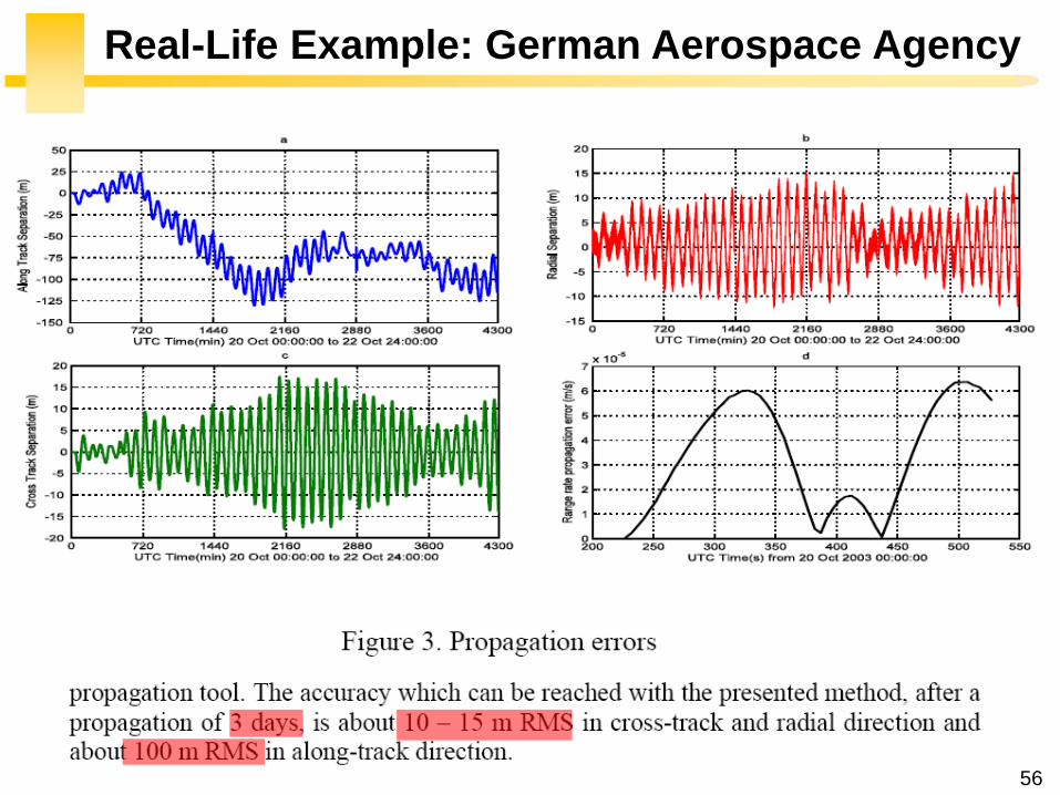
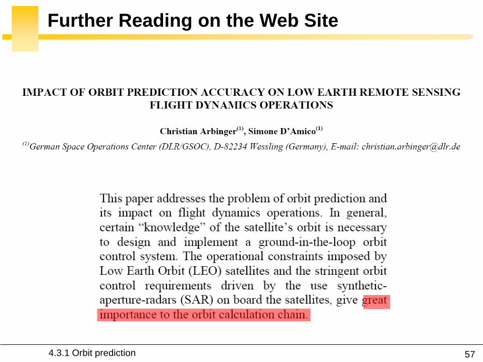
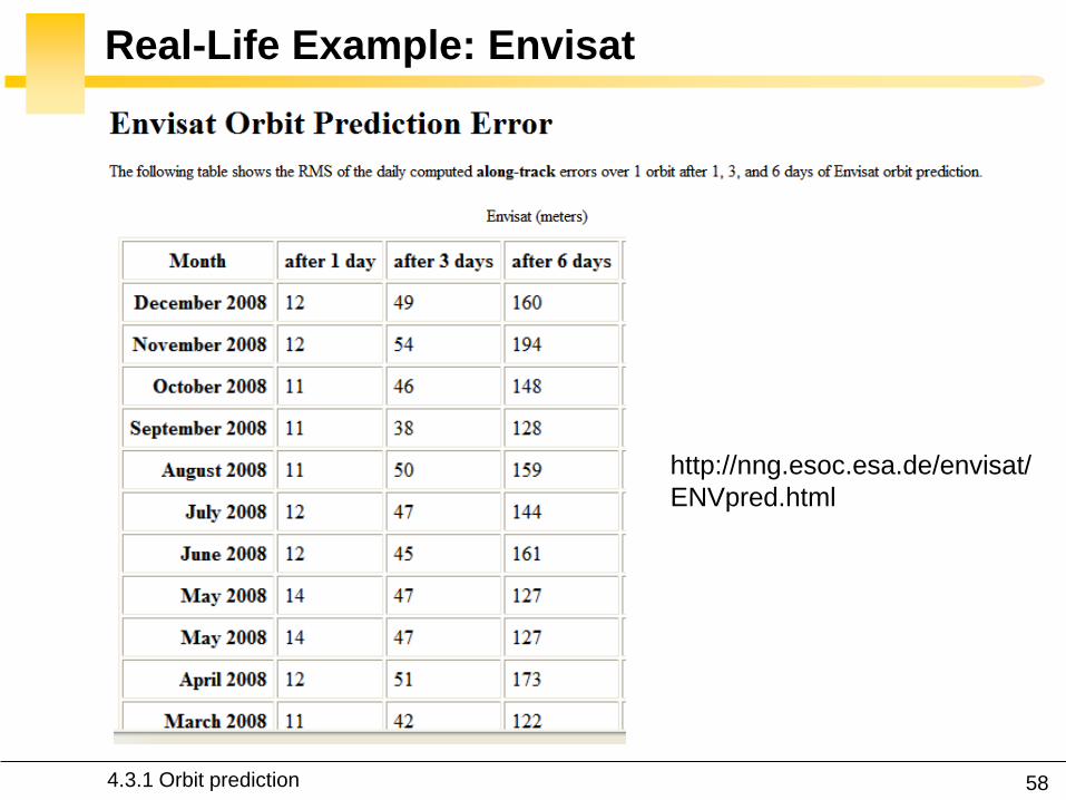
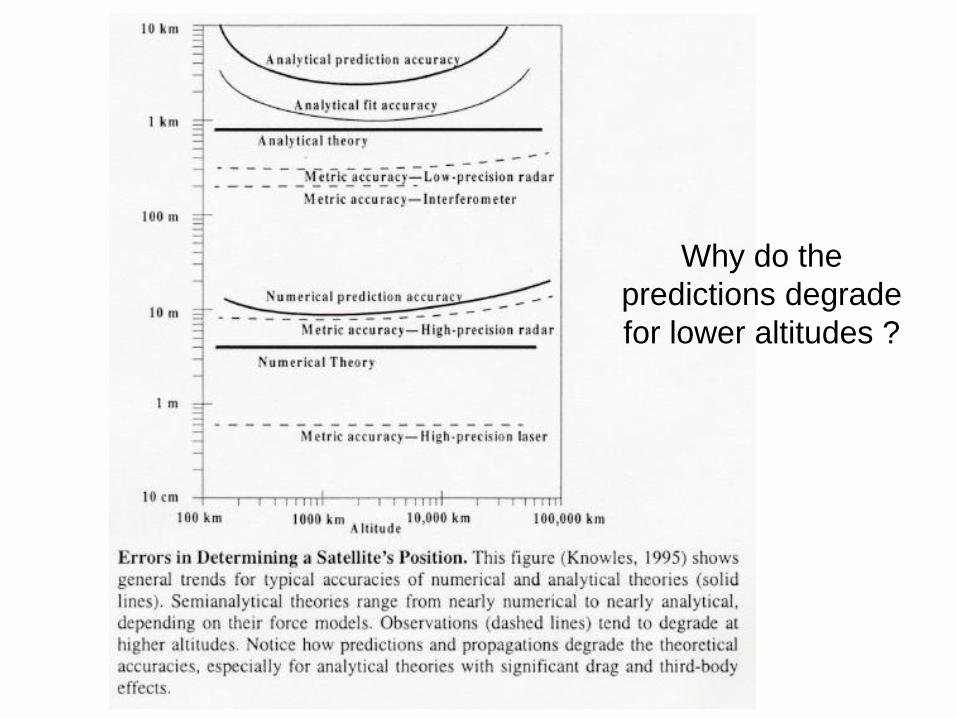
60
NASA began the first complex numerical integrations
during the late 1960s and early 1970s
Did you Know
1969 1968
431 Orbit prediction
61
What is Numerical Integration
1n nt t t
3 perturbedr
r r a
Given
Compute
( ) ( )n nt tr r
1 1( ) ( )n nt t r r
432 Numerical integration
62
State-Space Formulation
3 perturbedr
r r a
( )f tu u
ru
r
6-dimensional
state vector
432 Numerical integration
63
How to Perform Numerical Integration
2( )( ) ( ) ( ) ( ) ( )
2
ss
n n n n n s
h hf t h f t hf t f t f t R
s
Taylor series expansion
( )ntu
1( )nt u
432 Numerical integration
64
First-Order Taylor Approximation (Euler)
1
( ) ( ) ( )
( )
n n n
n n n n
t t t t t
t f t
u u u
u u uEuler step
0 1 2 3 4 5 60
5
10
15
20
25
30
35
40
Time t (s)
x(t
)=t2
Exact solution
The stepsize has to be extremely
small for accurate predictions
and it is necessary to develop
more effective algorithms
along the tangent
432 Numerical integration
65
Numerical Integration Methods
1 1 1
1 0
m m
n j n j j n j
j j
t
u u u
0 0
Implicit the solution method becomes
iterative in the nonlinear case
0 0 Explicit un+1 can be deduced directly from
the results at the previous time steps
=0
for 1
j j
j
Single-step the system at time tn+1
only depends on the previous state tn
State vector
0
for 1
j j
j
Multi-step the system at time tn+1 depends
several previous states tntn-1etc
432 Numerical integration
66
Examples Implicit vs Explicit
Trapezoidal rule (implicit)
nt 1nt
Euler forward (explicit)
nt 1nt
Euler backward (implicit)
nt 1nt
1n n nt u u u
1 1n n nt u u u
1
12
n n
n n t
u uu u
r
r
r
432 Numerical integration
67
A variety of methods has been applied in astrodynamics
Each of these methods has its own advantages and
drawbacks
Accuracy what is the order of the integration scheme
Efficiency how many function calls
Versatility can it be applied to a wide range of problems
Complexity is it easy to implement and use
Step size automatic step size control
Why Different Methods
431 Orbit prediction
68
Runge-Kutta Family Single-Step
Perhaps the most well-known numerical integrator
Difference with traditional Taylor series integrators the RK
family only requires the first derivative but several
evaluations are needed to move forward one step in time
Different variants explicit embedded etc
433 Single-step methods Runge-Kutta
69
Runge-Kutta Family Single-Step
with ( ) ( )t f tu u 0 0( )t u u
1
1
s
n n i i
i
t b
u u k
1 1
1
1
2
n n
i
i n ij j n i
j
f t c t
f t a t c t i s
k u
k u k
Slopes at
various points
within the
integration step
433 Single-step methods Runge-Kutta
70
Runge-Kutta Family Single-Step
Butcher Tableau
The Runge-Kutta methods are fully described by the
coefficients
c1
c2
cs
a21
as1
b1
as2
b2
ass-1
bs-1 hellip
hellip
hellip hellip hellip
bs
1
1
1
1
1
0
s
i
i
i
i ij
j
b
c
c a
433 Single-step methods Runge-Kutta
71
RK4 (Explicit)
1 2 3 41
2 2
6n n t
k k k ku u
Butcher Tableau
1
2 1
3 2
4 3
2 2
2 2
n n
n n
n n
n n
f t
t tf t
t tf t
f t t t
k u
k u k
k u k
k u k
433 Single-step methods Runge-Kutta
72
RK4 (Explicit)
1 2 3 41
2 2
6n n t
k k k ku u
1
2 1
3 2
4 3
2 2
2 2
n n
n n
n n
n n
f t
t tf t
t tf t
f t t t
k u
k u k
k u k
k u k
Slope at the beginning
Slope at the midpoint (k1 is
used to determine the value
of u Euler)
Slope at the midpoint (k2 is
now used)
Slope at the end
Estimated slope
(weighted average)
433 Single-step methods Runge-Kutta
73
RK4 (Explicit)
nt 2nt t nt t
1k3k
2k
4k
Estimate at new
time
u
433 Single-step methods Runge-Kutta
74
RK4 (Explicit)
The local truncation error for a 4th order RK is O(h5)
The accuracy is comparable to that of a 4th order Taylor
series but the Runge-Kutta method avoids the
calculation of higher-order derivatives
Easy to use and implement
The step size is fixed
433 Single-step methods Runge-Kutta
75
RK4 in STK
433 Single-step methods Runge-Kutta
76
Embedded Methods
They produce an estimate of the local truncation error
adjust the step size to keep local truncation errors
within some tolerances
This is done by having two methods in the tableau one with
order p and one with order p+1 with the same set of
function evaluations
( 1) ( 1) ( 1)
1
1
sp p p
n n i i
i
t b
u u k
( ) ( ) ( )
1
1
sp p p
n n i i
i
t b
u u k
433 Single-step methods Runge-Kutta
77
Embedded Methods
The two different approximations for the solution at each
step are compared
If the two answers are in close agreement the approximation is
accepted
If the two answers do not agree to a specified accuracy the step
size is reduced
If the answers agree to more significant digits than required the
step size is increased
433 Single-step methods Runge-Kutta
78
Ode45 in Matlab Simulink
Runge-Kutta (45) pair of Dormand and Prince
Variable step size
Matlab help This should be the first solver you try
433 Single-step methods Runge-Kutta
79
Ode45 in Matlab Simulink
edit ode45
433 Single-step methods Runge-Kutta
80
Ode45 in Matlab Simulink
Be very careful with the default parameters
options = odeset(RelTol1e-8AbsTol1e-8)
433 Single-step methods Runge-Kutta
81
RKF 7(8) Default Method in STK
Runge-Kutta-Fehlberg integration method of 7th order
with 8th order error control for the integration step size
433 Single-step methods Runge-Kutta
83
Multi-Step Methods (Predictor-Corrector)
They estimate the state over time using previously
determined back values of the solution
Unlike RK methods they only perform one evaluation for
each step forward but they usually have a predictor and a
corrector formula
Adams() ndash Bashforth - Moulton Gauss - Jackson
() The first with Le Verrier to predict the existence and position of Neptune
434 Multi-step methods
84
Multi-Step Methods Principle
( ) ( )t f tu u1
1( ) ( ) ( ) n
n
t
n nt
t t f t dt
u u u
unknown
Replace it by a
polynomial that
interpolates the
previous values Four function values
interpolated by a
third-order polynomial
t
u
434 Multi-step methods
85
Multi-Step Methods Initiation
with ( ) ( )t f tu u 0 0( )t u u
What is the inherent problem
t
u
434 Multi-step methods
86
Multi-Step Methods Initiation
Because these methods require back values they are not
self-starting
One may for instance use of a single-step method to
compute the first four values
434 Multi-step methods
87
Gauss-Jackson in STK
One of the most recommendable fixed-stepsize multistep
methods for orbit computations
88
Integrator Selection
435 Integrator and step size selection
Montenbruck and Gill
Satellite orbits Springer
2000
89
Integrator Selection
Pros
Very fast
Cons
Special starting procedure
Fixed time steps
Error control
Pros
Plug and play
Error control
Cons
Slower
Multi-step Single step
435 Integrator and step size selection
90
Why is the Step Size So Critical
Theoretical arguments
1 The accuracy and the stability of the algorithm are
directly related to the step size
2 Nonlinear equations of motion
Data for Landsat 4 and 6 in circular orbits around 800km
indicates that a one-minute step size yields about 47m
error
A three-minute step size produces about a 900m error
435 Integrator and step size selection
91
Why is the Step Size So Critical
More practical arguments
1 The computation time is directly related to the
step size
2 The particular choice of step size depends on the
most rapidly varying component in the disturbing
functions (eg 50 x 50 gravity field)
435 Integrator and step size selection
92
Appropriate Step Size
The problem of determining an appropriate step size is a
challenge in any numerical process
Fixed step size (rule of thumb for standard
applications)
But an algorithm with variable step size is really
helpful The step size is chosen in such a way that
each step contributes uniformly to the total integration
error
100
orbitTt
435 Integrator and step size selection
93
Three Examples XMM OUFTI-1 ISS
Can you plot the step size vs true anomaly
435 Integrator and step size selection
94
XMM Report in STK
435 Integrator and step size selection
95
XMM (e~08)
0 50 100 150 200 250 300 350 4000
1000
2000
3000
4000
5000
6000
True anomaly (deg)
Ste
p s
ize
(s)
435 Integrator and step size selection
96
ISS(e~0)
435 Integrator and step size selection
0 50 100 150 200 250 300 350 40030
35
40
45
50
55
60
65
70
True anomaly (deg)
Ste
p s
ize
(s)
97
ldquoDifficultrdquo Orbits
Automatic time step is especially nice on highly eccentric
orbits (Molniya XMM) These orbits are best computed
using variable step sizes to maintain some given level of
accuracy
Without this variable step size we waste a lot of time near
apoapsis when the integration is taking too small a step
Likewise the integrator may not be using a small enough step
size at periapsis where the satellite is traveling fast
435 Integrator and step size selection
98
HPOP Propagator ISS Example
1 Earthrsquos oblateness only
2 Drag only
3 Sun and moon only
4 SRP only
5 All together
436 ISS example
99
Earthrsquos Oblateness Only Ω
HPOP
J2
2-body
436 ISS example
100
Earthrsquos Oblateness Only i Ω a
HPOP with central body (20 + WGS84_EGM96)
(without dragSRPSun and Moon)
436 ISS example
101
Drag Only i Ω a
HPOP with drag ndash Harris Priester
(without oblatenessSRPSun and Moon)
436 ISS example
102
Drag Relationship with Eclipses
103
SRP Only i Ω a
HPOP with SRP
(without oblatenessdragSun and Moon)
436 ISS example
104
SRP Relationship with Eclipses
105
All Perturbations Together
436 ISS example
106
4 Non-Keplerian Motion
2
2
(1 )
sin
sin 1 cos
a e
N
i e
44 Geostationary satellites
107
Practical Example GEO Satellites
Nice illustration of
1 Perturbations of the 2-body problem
2 Secular and periodic contributions
3 Accuracy required by practical applications
4 The need for orbit correction and thrust forces
And it is a real-life example (telecommunications
meteorology)
44 GEO satellites
108
Three Main Perturbations for GEO Satellites
44 GEO satellites
1 Non-spherical Earth
2 SRP
3 Sun and Moon
109
Station Keeping of GEO Satellites
The effect of the perturbations is to cause the spacecraft
to drift away from its nominal station If the drift was
allowed to build up unchecked the spacecraft could
become useless
A station-keeping box is defined by a longitude and a
maximum authorized distance for satellite excursions in
longitude and latitude
For instance TC2 -8ordm plusmn 007ordm EW plusmn 005ordm NS
44 GEO satellites
110
East-West and North-South Drift
44 GEO satellites
NS drift
EW drift
What are the perturbations generating these drifts
111
East-West Drift
44 GEO satellites
A GEO satellite drifts in longitude due to the influence of
two main perturbations
1 The elliptic nature of the Earthrsquos equatorial cross-
section J22 (and not from the NS oblateness J2)
2
ΔV
ΔV vsat
vsat SRP
112
East-West Drift due to Equatorial Ellipticity
44 GEO satellites
113
East-West Drift due to Equatorial Ellipticity
44 GEO satellites
114
East-West Drift HPOP (20) vs HPOP (22)
44 GEO satellites
115
East-West Drift Stable Equilibirum
HPOP with 22
(without Sun and moonSRPdrag)
116
East-West Drift Stable Equilibirum
HPOP with 22
(without Sun and moonSRPdrag)
117
East-West Drift Stable Equilibirum
HPOP with 22
(without Sun and moonSRPdrag)
118
North-South Drift
The perturbations caused by the Sun and the Moon are
predominantly out-of-plane effects causing a change in
the inclination and in the right ascension of the orbit
ascending node
Similar effects on the orbit to those of the Earthrsquos
oblateness (but here with respect to the ecliptic)
A GEO satellite therefore drifts in latitude with a
fundamental period equal to the orbit period
119
North-South Drift
Period
HPOP with Sun and Moon
(without oblatenessSRPdrag)
120
North-South Drift
Period
HPOP with Sun and Moon
(without oblatenessSRPdrag)
121
Thrust Forces for Stationkeeping
GEO spacecraft require continual stationkeeping to stay
within the authorized box using onboard thrusters
44 GEO satellites
122
42 ANALYTIC TREATMENT
421 Variation of parameters
422 Non-spherical Earth
423 J2 propagator in STK
424 Atmospheric drag
425 Third-body perturbations
426 SGP4 propagator in STK
427 Solar radiation pressure
4 Non-Keplerian Motion
43 NUMERICAL METHODS
431 Orbit prediction
432 Numerical integration
433 Single-step methods Runge-Kutta
434 Multi-step methods
435 Integrator and step size selection
436 ISS example
44 GEOSTATIONARY SATELLITES
Gaeumltan Kerschen
Space Structures amp
Systems Lab (S3L)
4B Non-Keplerian Motion
Astrodynamics (AERO0024)
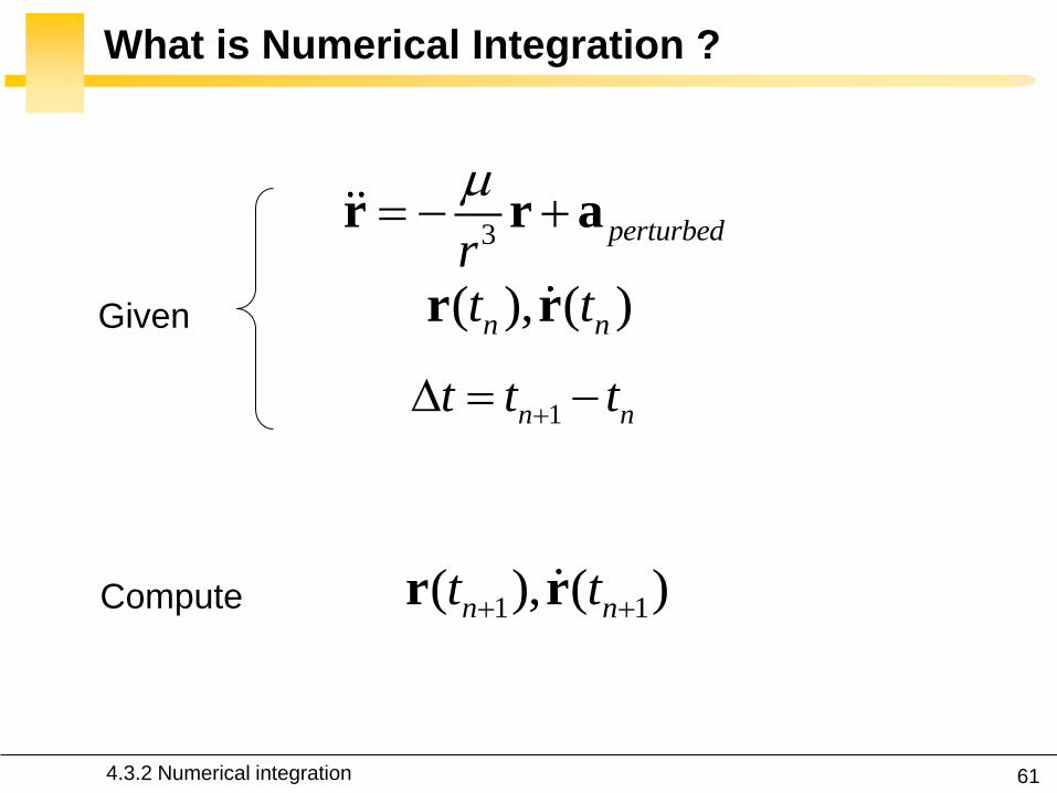
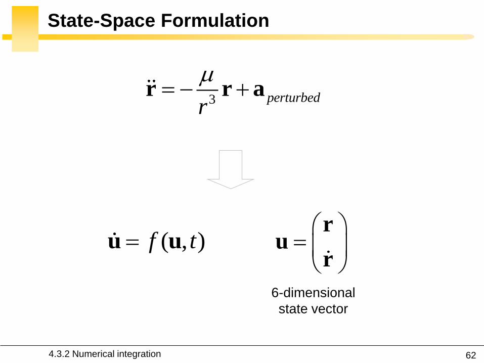
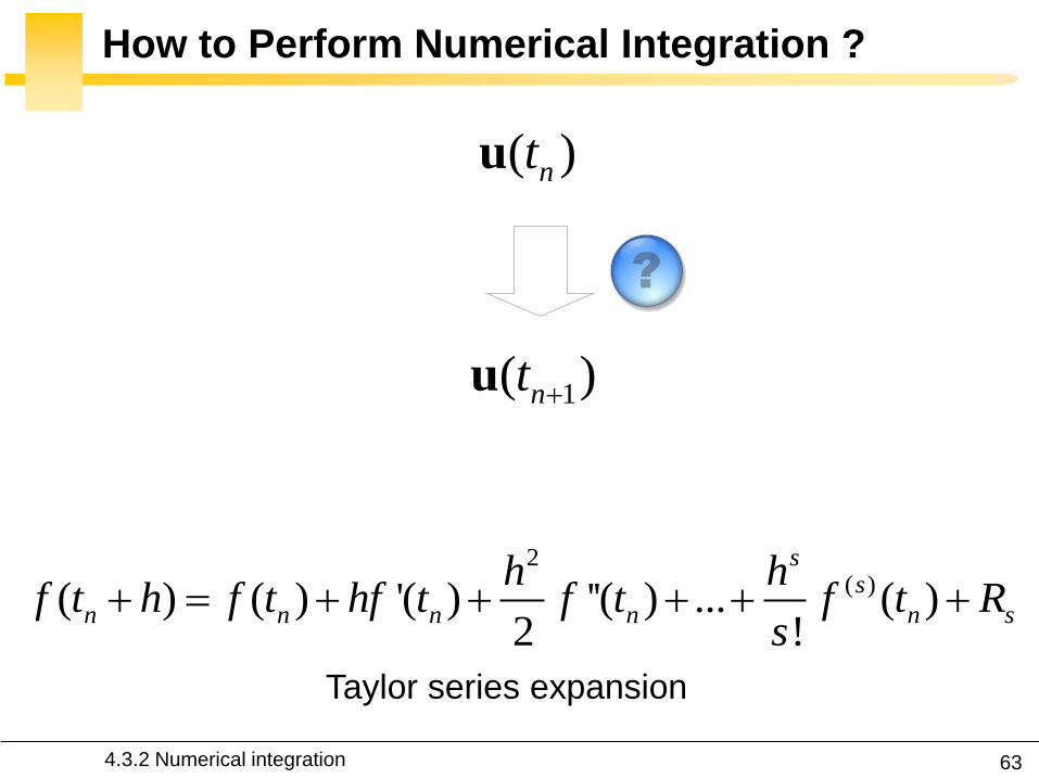
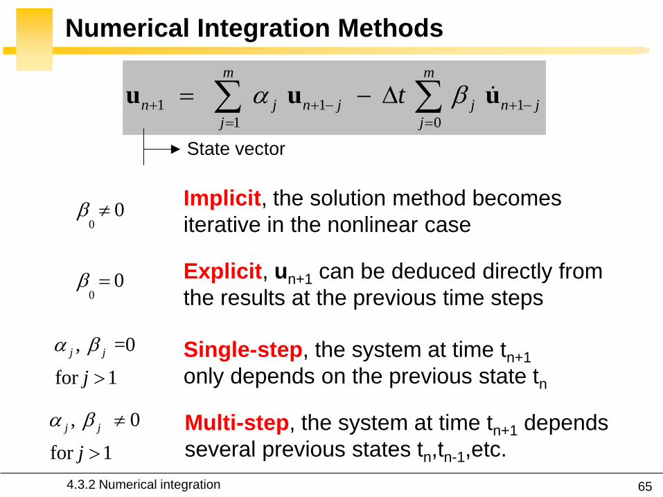
65
Numerical Integration Methods
1 1 1
1 0
m m
n j n j j n j
j j
t
u u u
0 0
Implicit the solution method becomes
iterative in the nonlinear case
0 0 Explicit un+1 can be deduced directly from
the results at the previous time steps
=0
for 1
j j
j
Single-step the system at time tn+1
only depends on the previous state tn
State vector
0
for 1
j j
j
Multi-step the system at time tn+1 depends
several previous states tntn-1etc
432 Numerical integration
66
Examples Implicit vs Explicit
Trapezoidal rule (implicit)
nt 1nt
Euler forward (explicit)
nt 1nt
Euler backward (implicit)
nt 1nt
1n n nt u u u
1 1n n nt u u u
1
12
n n
n n t
u uu u
r
r
r
432 Numerical integration
67
A variety of methods has been applied in astrodynamics
Each of these methods has its own advantages and
drawbacks
Accuracy what is the order of the integration scheme
Efficiency how many function calls
Versatility can it be applied to a wide range of problems
Complexity is it easy to implement and use
Step size automatic step size control
Why Different Methods
431 Orbit prediction
68
Runge-Kutta Family Single-Step
Perhaps the most well-known numerical integrator
Difference with traditional Taylor series integrators the RK
family only requires the first derivative but several
evaluations are needed to move forward one step in time
Different variants explicit embedded etc
433 Single-step methods Runge-Kutta
69
Runge-Kutta Family Single-Step
with ( ) ( )t f tu u 0 0( )t u u
1
1
s
n n i i
i
t b
u u k
1 1
1
1
2
n n
i
i n ij j n i
j
f t c t
f t a t c t i s
k u
k u k
Slopes at
various points
within the
integration step
433 Single-step methods Runge-Kutta
70
Runge-Kutta Family Single-Step
Butcher Tableau
The Runge-Kutta methods are fully described by the
coefficients
c1
c2
cs
a21
as1
b1
as2
b2
ass-1
bs-1 hellip
hellip
hellip hellip hellip
bs
1
1
1
1
1
0
s
i
i
i
i ij
j
b
c
c a
433 Single-step methods Runge-Kutta
71
RK4 (Explicit)
1 2 3 41
2 2
6n n t
k k k ku u
Butcher Tableau
1
2 1
3 2
4 3
2 2
2 2
n n
n n
n n
n n
f t
t tf t
t tf t
f t t t
k u
k u k
k u k
k u k
433 Single-step methods Runge-Kutta
72
RK4 (Explicit)
1 2 3 41
2 2
6n n t
k k k ku u
1
2 1
3 2
4 3
2 2
2 2
n n
n n
n n
n n
f t
t tf t
t tf t
f t t t
k u
k u k
k u k
k u k
Slope at the beginning
Slope at the midpoint (k1 is
used to determine the value
of u Euler)
Slope at the midpoint (k2 is
now used)
Slope at the end
Estimated slope
(weighted average)
433 Single-step methods Runge-Kutta
73
RK4 (Explicit)
nt 2nt t nt t
1k3k
2k
4k
Estimate at new
time
u
433 Single-step methods Runge-Kutta
74
RK4 (Explicit)
The local truncation error for a 4th order RK is O(h5)
The accuracy is comparable to that of a 4th order Taylor
series but the Runge-Kutta method avoids the
calculation of higher-order derivatives
Easy to use and implement
The step size is fixed
433 Single-step methods Runge-Kutta
75
RK4 in STK
433 Single-step methods Runge-Kutta
76
Embedded Methods
They produce an estimate of the local truncation error
adjust the step size to keep local truncation errors
within some tolerances
This is done by having two methods in the tableau one with
order p and one with order p+1 with the same set of
function evaluations
( 1) ( 1) ( 1)
1
1
sp p p
n n i i
i
t b
u u k
( ) ( ) ( )
1
1
sp p p
n n i i
i
t b
u u k
433 Single-step methods Runge-Kutta
77
Embedded Methods
The two different approximations for the solution at each
step are compared
If the two answers are in close agreement the approximation is
accepted
If the two answers do not agree to a specified accuracy the step
size is reduced
If the answers agree to more significant digits than required the
step size is increased
433 Single-step methods Runge-Kutta
78
Ode45 in Matlab Simulink
Runge-Kutta (45) pair of Dormand and Prince
Variable step size
Matlab help This should be the first solver you try
433 Single-step methods Runge-Kutta
79
Ode45 in Matlab Simulink
edit ode45
433 Single-step methods Runge-Kutta
80
Ode45 in Matlab Simulink
Be very careful with the default parameters
options = odeset(RelTol1e-8AbsTol1e-8)
433 Single-step methods Runge-Kutta
81
RKF 7(8) Default Method in STK
Runge-Kutta-Fehlberg integration method of 7th order
with 8th order error control for the integration step size
433 Single-step methods Runge-Kutta
83
Multi-Step Methods (Predictor-Corrector)
They estimate the state over time using previously
determined back values of the solution
Unlike RK methods they only perform one evaluation for
each step forward but they usually have a predictor and a
corrector formula
Adams() ndash Bashforth - Moulton Gauss - Jackson
() The first with Le Verrier to predict the existence and position of Neptune
434 Multi-step methods
84
Multi-Step Methods Principle
( ) ( )t f tu u1
1( ) ( ) ( ) n
n
t
n nt
t t f t dt
u u u
unknown
Replace it by a
polynomial that
interpolates the
previous values Four function values
interpolated by a
third-order polynomial
t
u
434 Multi-step methods
85
Multi-Step Methods Initiation
with ( ) ( )t f tu u 0 0( )t u u
What is the inherent problem
t
u
434 Multi-step methods
86
Multi-Step Methods Initiation
Because these methods require back values they are not
self-starting
One may for instance use of a single-step method to
compute the first four values
434 Multi-step methods
87
Gauss-Jackson in STK
One of the most recommendable fixed-stepsize multistep
methods for orbit computations
88
Integrator Selection
435 Integrator and step size selection
Montenbruck and Gill
Satellite orbits Springer
2000
89
Integrator Selection
Pros
Very fast
Cons
Special starting procedure
Fixed time steps
Error control
Pros
Plug and play
Error control
Cons
Slower
Multi-step Single step
435 Integrator and step size selection
90
Why is the Step Size So Critical
Theoretical arguments
1 The accuracy and the stability of the algorithm are
directly related to the step size
2 Nonlinear equations of motion
Data for Landsat 4 and 6 in circular orbits around 800km
indicates that a one-minute step size yields about 47m
error
A three-minute step size produces about a 900m error
435 Integrator and step size selection
91
Why is the Step Size So Critical
More practical arguments
1 The computation time is directly related to the
step size
2 The particular choice of step size depends on the
most rapidly varying component in the disturbing
functions (eg 50 x 50 gravity field)
435 Integrator and step size selection
92
Appropriate Step Size
The problem of determining an appropriate step size is a
challenge in any numerical process
Fixed step size (rule of thumb for standard
applications)
But an algorithm with variable step size is really
helpful The step size is chosen in such a way that
each step contributes uniformly to the total integration
error
100
orbitTt
435 Integrator and step size selection
93
Three Examples XMM OUFTI-1 ISS
Can you plot the step size vs true anomaly
435 Integrator and step size selection
94
XMM Report in STK
435 Integrator and step size selection
95
XMM (e~08)
0 50 100 150 200 250 300 350 4000
1000
2000
3000
4000
5000
6000
True anomaly (deg)
Ste
p s
ize
(s)
435 Integrator and step size selection
96
ISS(e~0)
435 Integrator and step size selection
0 50 100 150 200 250 300 350 40030
35
40
45
50
55
60
65
70
True anomaly (deg)
Ste
p s
ize
(s)
97
ldquoDifficultrdquo Orbits
Automatic time step is especially nice on highly eccentric
orbits (Molniya XMM) These orbits are best computed
using variable step sizes to maintain some given level of
accuracy
Without this variable step size we waste a lot of time near
apoapsis when the integration is taking too small a step
Likewise the integrator may not be using a small enough step
size at periapsis where the satellite is traveling fast
435 Integrator and step size selection
98
HPOP Propagator ISS Example
1 Earthrsquos oblateness only
2 Drag only
3 Sun and moon only
4 SRP only
5 All together
436 ISS example
99
Earthrsquos Oblateness Only Ω
HPOP
J2
2-body
436 ISS example
100
Earthrsquos Oblateness Only i Ω a
HPOP with central body (20 + WGS84_EGM96)
(without dragSRPSun and Moon)
436 ISS example
101
Drag Only i Ω a
HPOP with drag ndash Harris Priester
(without oblatenessSRPSun and Moon)
436 ISS example
102
Drag Relationship with Eclipses
103
SRP Only i Ω a
HPOP with SRP
(without oblatenessdragSun and Moon)
436 ISS example
104
SRP Relationship with Eclipses
105
All Perturbations Together
436 ISS example
106
4 Non-Keplerian Motion
2
2
(1 )
sin
sin 1 cos
a e
N
i e
44 Geostationary satellites
107
Practical Example GEO Satellites
Nice illustration of
1 Perturbations of the 2-body problem
2 Secular and periodic contributions
3 Accuracy required by practical applications
4 The need for orbit correction and thrust forces
And it is a real-life example (telecommunications
meteorology)
44 GEO satellites
108
Three Main Perturbations for GEO Satellites
44 GEO satellites
1 Non-spherical Earth
2 SRP
3 Sun and Moon
109
Station Keeping of GEO Satellites
The effect of the perturbations is to cause the spacecraft
to drift away from its nominal station If the drift was
allowed to build up unchecked the spacecraft could
become useless
A station-keeping box is defined by a longitude and a
maximum authorized distance for satellite excursions in
longitude and latitude
For instance TC2 -8ordm plusmn 007ordm EW plusmn 005ordm NS
44 GEO satellites
110
East-West and North-South Drift
44 GEO satellites
NS drift
EW drift
What are the perturbations generating these drifts
111
East-West Drift
44 GEO satellites
A GEO satellite drifts in longitude due to the influence of
two main perturbations
1 The elliptic nature of the Earthrsquos equatorial cross-
section J22 (and not from the NS oblateness J2)
2
ΔV
ΔV vsat
vsat SRP
112
East-West Drift due to Equatorial Ellipticity
44 GEO satellites
113
East-West Drift due to Equatorial Ellipticity
44 GEO satellites
114
East-West Drift HPOP (20) vs HPOP (22)
44 GEO satellites
115
East-West Drift Stable Equilibirum
HPOP with 22
(without Sun and moonSRPdrag)
116
East-West Drift Stable Equilibirum
HPOP with 22
(without Sun and moonSRPdrag)
117
East-West Drift Stable Equilibirum
HPOP with 22
(without Sun and moonSRPdrag)
118
North-South Drift
The perturbations caused by the Sun and the Moon are
predominantly out-of-plane effects causing a change in
the inclination and in the right ascension of the orbit
ascending node
Similar effects on the orbit to those of the Earthrsquos
oblateness (but here with respect to the ecliptic)
A GEO satellite therefore drifts in latitude with a
fundamental period equal to the orbit period
119
North-South Drift
Period
HPOP with Sun and Moon
(without oblatenessSRPdrag)
120
North-South Drift
Period
HPOP with Sun and Moon
(without oblatenessSRPdrag)
121
Thrust Forces for Stationkeeping
GEO spacecraft require continual stationkeeping to stay
within the authorized box using onboard thrusters
44 GEO satellites
122
42 ANALYTIC TREATMENT
421 Variation of parameters
422 Non-spherical Earth
423 J2 propagator in STK
424 Atmospheric drag
425 Third-body perturbations
426 SGP4 propagator in STK
427 Solar radiation pressure
4 Non-Keplerian Motion
43 NUMERICAL METHODS
431 Orbit prediction
432 Numerical integration
433 Single-step methods Runge-Kutta
434 Multi-step methods
435 Integrator and step size selection
436 ISS example
44 GEOSTATIONARY SATELLITES
Gaeumltan Kerschen
Space Structures amp
Systems Lab (S3L)
4B Non-Keplerian Motion
Astrodynamics (AERO0024)
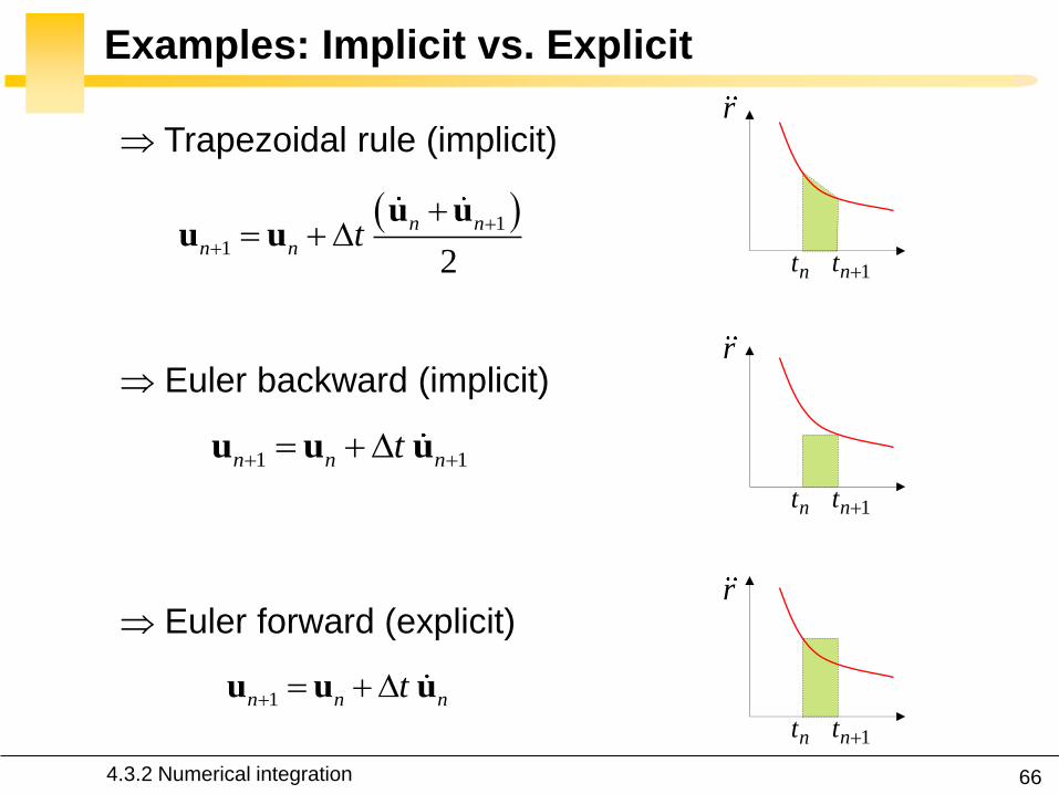
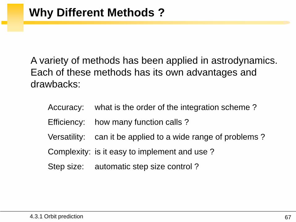
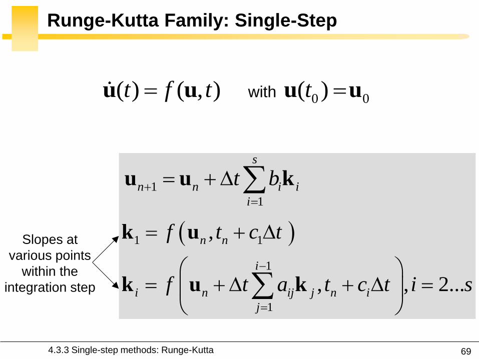
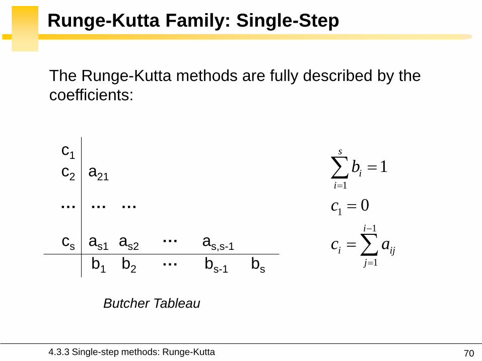
70
Runge-Kutta Family Single-Step
Butcher Tableau
The Runge-Kutta methods are fully described by the
coefficients
c1
c2
cs
a21
as1
b1
as2
b2
ass-1
bs-1 hellip
hellip
hellip hellip hellip
bs
1
1
1
1
1
0
s
i
i
i
i ij
j
b
c
c a
433 Single-step methods Runge-Kutta
71
RK4 (Explicit)
1 2 3 41
2 2
6n n t
k k k ku u
Butcher Tableau
1
2 1
3 2
4 3
2 2
2 2
n n
n n
n n
n n
f t
t tf t
t tf t
f t t t
k u
k u k
k u k
k u k
433 Single-step methods Runge-Kutta
72
RK4 (Explicit)
1 2 3 41
2 2
6n n t
k k k ku u
1
2 1
3 2
4 3
2 2
2 2
n n
n n
n n
n n
f t
t tf t
t tf t
f t t t
k u
k u k
k u k
k u k
Slope at the beginning
Slope at the midpoint (k1 is
used to determine the value
of u Euler)
Slope at the midpoint (k2 is
now used)
Slope at the end
Estimated slope
(weighted average)
433 Single-step methods Runge-Kutta
73
RK4 (Explicit)
nt 2nt t nt t
1k3k
2k
4k
Estimate at new
time
u
433 Single-step methods Runge-Kutta
74
RK4 (Explicit)
The local truncation error for a 4th order RK is O(h5)
The accuracy is comparable to that of a 4th order Taylor
series but the Runge-Kutta method avoids the
calculation of higher-order derivatives
Easy to use and implement
The step size is fixed
433 Single-step methods Runge-Kutta
75
RK4 in STK
433 Single-step methods Runge-Kutta
76
Embedded Methods
They produce an estimate of the local truncation error
adjust the step size to keep local truncation errors
within some tolerances
This is done by having two methods in the tableau one with
order p and one with order p+1 with the same set of
function evaluations
( 1) ( 1) ( 1)
1
1
sp p p
n n i i
i
t b
u u k
( ) ( ) ( )
1
1
sp p p
n n i i
i
t b
u u k
433 Single-step methods Runge-Kutta
77
Embedded Methods
The two different approximations for the solution at each
step are compared
If the two answers are in close agreement the approximation is
accepted
If the two answers do not agree to a specified accuracy the step
size is reduced
If the answers agree to more significant digits than required the
step size is increased
433 Single-step methods Runge-Kutta
78
Ode45 in Matlab Simulink
Runge-Kutta (45) pair of Dormand and Prince
Variable step size
Matlab help This should be the first solver you try
433 Single-step methods Runge-Kutta
79
Ode45 in Matlab Simulink
edit ode45
433 Single-step methods Runge-Kutta
80
Ode45 in Matlab Simulink
Be very careful with the default parameters
options = odeset(RelTol1e-8AbsTol1e-8)
433 Single-step methods Runge-Kutta
81
RKF 7(8) Default Method in STK
Runge-Kutta-Fehlberg integration method of 7th order
with 8th order error control for the integration step size
433 Single-step methods Runge-Kutta
83
Multi-Step Methods (Predictor-Corrector)
They estimate the state over time using previously
determined back values of the solution
Unlike RK methods they only perform one evaluation for
each step forward but they usually have a predictor and a
corrector formula
Adams() ndash Bashforth - Moulton Gauss - Jackson
() The first with Le Verrier to predict the existence and position of Neptune
434 Multi-step methods
84
Multi-Step Methods Principle
( ) ( )t f tu u1
1( ) ( ) ( ) n
n
t
n nt
t t f t dt
u u u
unknown
Replace it by a
polynomial that
interpolates the
previous values Four function values
interpolated by a
third-order polynomial
t
u
434 Multi-step methods
85
Multi-Step Methods Initiation
with ( ) ( )t f tu u 0 0( )t u u
What is the inherent problem
t
u
434 Multi-step methods
86
Multi-Step Methods Initiation
Because these methods require back values they are not
self-starting
One may for instance use of a single-step method to
compute the first four values
434 Multi-step methods
87
Gauss-Jackson in STK
One of the most recommendable fixed-stepsize multistep
methods for orbit computations
88
Integrator Selection
435 Integrator and step size selection
Montenbruck and Gill
Satellite orbits Springer
2000
89
Integrator Selection
Pros
Very fast
Cons
Special starting procedure
Fixed time steps
Error control
Pros
Plug and play
Error control
Cons
Slower
Multi-step Single step
435 Integrator and step size selection
90
Why is the Step Size So Critical
Theoretical arguments
1 The accuracy and the stability of the algorithm are
directly related to the step size
2 Nonlinear equations of motion
Data for Landsat 4 and 6 in circular orbits around 800km
indicates that a one-minute step size yields about 47m
error
A three-minute step size produces about a 900m error
435 Integrator and step size selection
91
Why is the Step Size So Critical
More practical arguments
1 The computation time is directly related to the
step size
2 The particular choice of step size depends on the
most rapidly varying component in the disturbing
functions (eg 50 x 50 gravity field)
435 Integrator and step size selection
92
Appropriate Step Size
The problem of determining an appropriate step size is a
challenge in any numerical process
Fixed step size (rule of thumb for standard
applications)
But an algorithm with variable step size is really
helpful The step size is chosen in such a way that
each step contributes uniformly to the total integration
error
100
orbitTt
435 Integrator and step size selection
93
Three Examples XMM OUFTI-1 ISS
Can you plot the step size vs true anomaly
435 Integrator and step size selection
94
XMM Report in STK
435 Integrator and step size selection
95
XMM (e~08)
0 50 100 150 200 250 300 350 4000
1000
2000
3000
4000
5000
6000
True anomaly (deg)
Ste
p s
ize
(s)
435 Integrator and step size selection
96
ISS(e~0)
435 Integrator and step size selection
0 50 100 150 200 250 300 350 40030
35
40
45
50
55
60
65
70
True anomaly (deg)
Ste
p s
ize
(s)
97
ldquoDifficultrdquo Orbits
Automatic time step is especially nice on highly eccentric
orbits (Molniya XMM) These orbits are best computed
using variable step sizes to maintain some given level of
accuracy
Without this variable step size we waste a lot of time near
apoapsis when the integration is taking too small a step
Likewise the integrator may not be using a small enough step
size at periapsis where the satellite is traveling fast
435 Integrator and step size selection
98
HPOP Propagator ISS Example
1 Earthrsquos oblateness only
2 Drag only
3 Sun and moon only
4 SRP only
5 All together
436 ISS example
99
Earthrsquos Oblateness Only Ω
HPOP
J2
2-body
436 ISS example
100
Earthrsquos Oblateness Only i Ω a
HPOP with central body (20 + WGS84_EGM96)
(without dragSRPSun and Moon)
436 ISS example
101
Drag Only i Ω a
HPOP with drag ndash Harris Priester
(without oblatenessSRPSun and Moon)
436 ISS example
102
Drag Relationship with Eclipses
103
SRP Only i Ω a
HPOP with SRP
(without oblatenessdragSun and Moon)
436 ISS example
104
SRP Relationship with Eclipses
105
All Perturbations Together
436 ISS example
106
4 Non-Keplerian Motion
2
2
(1 )
sin
sin 1 cos
a e
N
i e
44 Geostationary satellites
107
Practical Example GEO Satellites
Nice illustration of
1 Perturbations of the 2-body problem
2 Secular and periodic contributions
3 Accuracy required by practical applications
4 The need for orbit correction and thrust forces
And it is a real-life example (telecommunications
meteorology)
44 GEO satellites
108
Three Main Perturbations for GEO Satellites
44 GEO satellites
1 Non-spherical Earth
2 SRP
3 Sun and Moon
109
Station Keeping of GEO Satellites
The effect of the perturbations is to cause the spacecraft
to drift away from its nominal station If the drift was
allowed to build up unchecked the spacecraft could
become useless
A station-keeping box is defined by a longitude and a
maximum authorized distance for satellite excursions in
longitude and latitude
For instance TC2 -8ordm plusmn 007ordm EW plusmn 005ordm NS
44 GEO satellites
110
East-West and North-South Drift
44 GEO satellites
NS drift
EW drift
What are the perturbations generating these drifts
111
East-West Drift
44 GEO satellites
A GEO satellite drifts in longitude due to the influence of
two main perturbations
1 The elliptic nature of the Earthrsquos equatorial cross-
section J22 (and not from the NS oblateness J2)
2
ΔV
ΔV vsat
vsat SRP
112
East-West Drift due to Equatorial Ellipticity
44 GEO satellites
113
East-West Drift due to Equatorial Ellipticity
44 GEO satellites
114
East-West Drift HPOP (20) vs HPOP (22)
44 GEO satellites
115
East-West Drift Stable Equilibirum
HPOP with 22
(without Sun and moonSRPdrag)
116
East-West Drift Stable Equilibirum
HPOP with 22
(without Sun and moonSRPdrag)
117
East-West Drift Stable Equilibirum
HPOP with 22
(without Sun and moonSRPdrag)
118
North-South Drift
The perturbations caused by the Sun and the Moon are
predominantly out-of-plane effects causing a change in
the inclination and in the right ascension of the orbit
ascending node
Similar effects on the orbit to those of the Earthrsquos
oblateness (but here with respect to the ecliptic)
A GEO satellite therefore drifts in latitude with a
fundamental period equal to the orbit period
119
North-South Drift
Period
HPOP with Sun and Moon
(without oblatenessSRPdrag)
120
North-South Drift
Period
HPOP with Sun and Moon
(without oblatenessSRPdrag)
121
Thrust Forces for Stationkeeping
GEO spacecraft require continual stationkeeping to stay
within the authorized box using onboard thrusters
44 GEO satellites
122
42 ANALYTIC TREATMENT
421 Variation of parameters
422 Non-spherical Earth
423 J2 propagator in STK
424 Atmospheric drag
425 Third-body perturbations
426 SGP4 propagator in STK
427 Solar radiation pressure
4 Non-Keplerian Motion
43 NUMERICAL METHODS
431 Orbit prediction
432 Numerical integration
433 Single-step methods Runge-Kutta
434 Multi-step methods
435 Integrator and step size selection
436 ISS example
44 GEOSTATIONARY SATELLITES
Gaeumltan Kerschen
Space Structures amp
Systems Lab (S3L)
4B Non-Keplerian Motion
Astrodynamics (AERO0024)
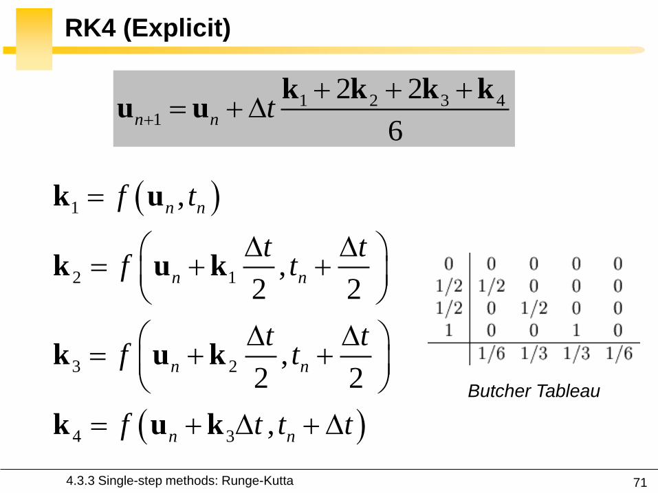
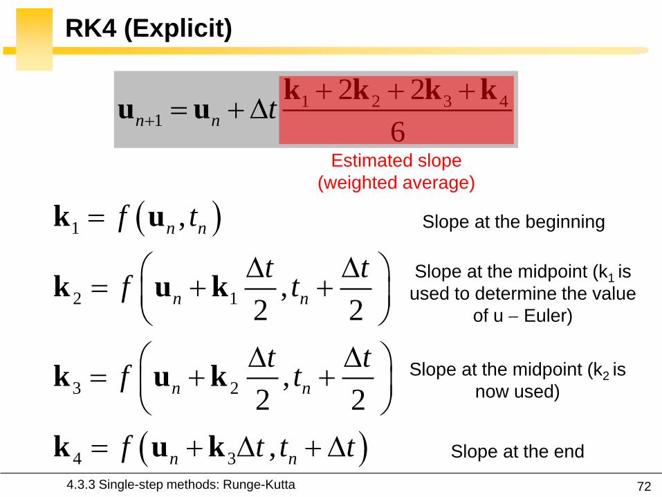
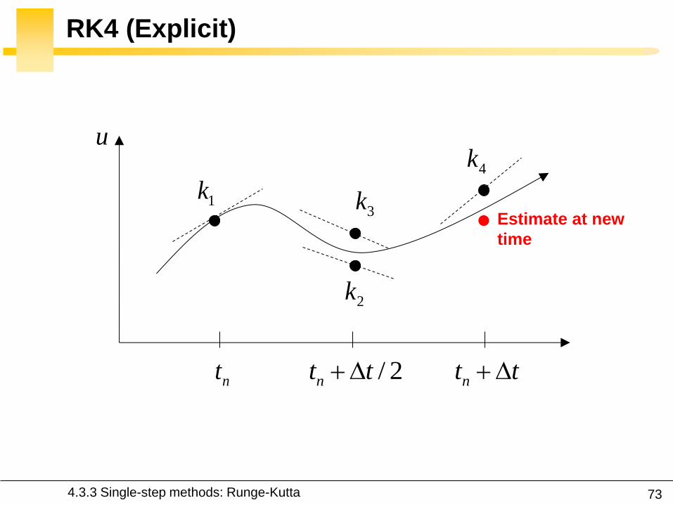
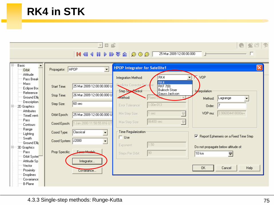
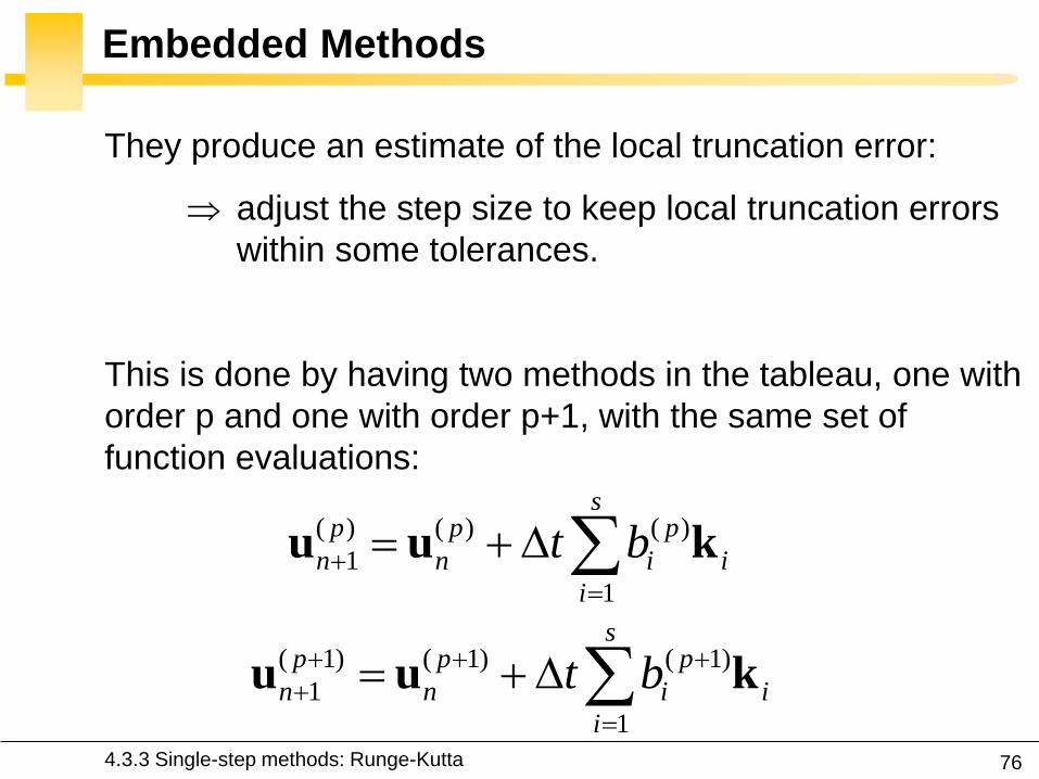
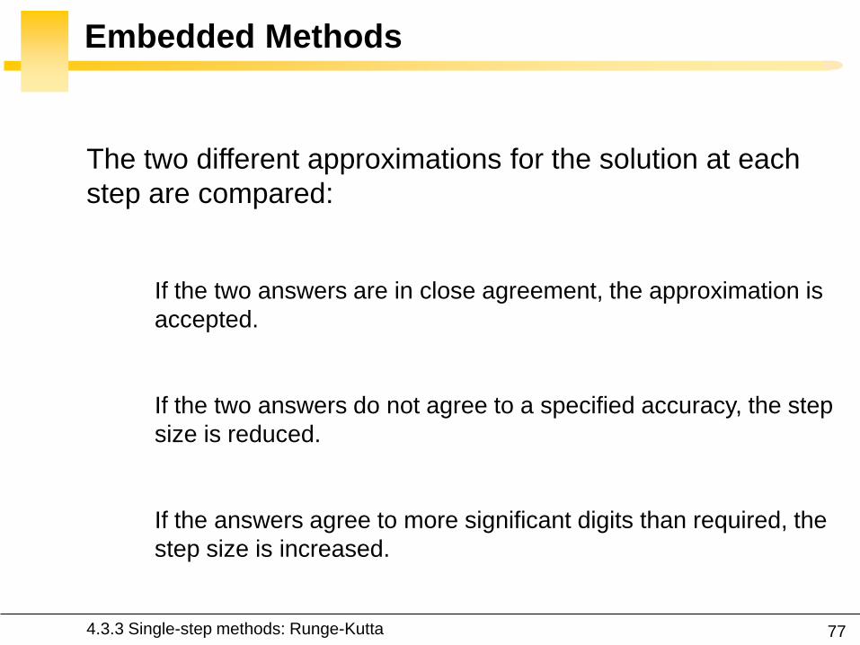
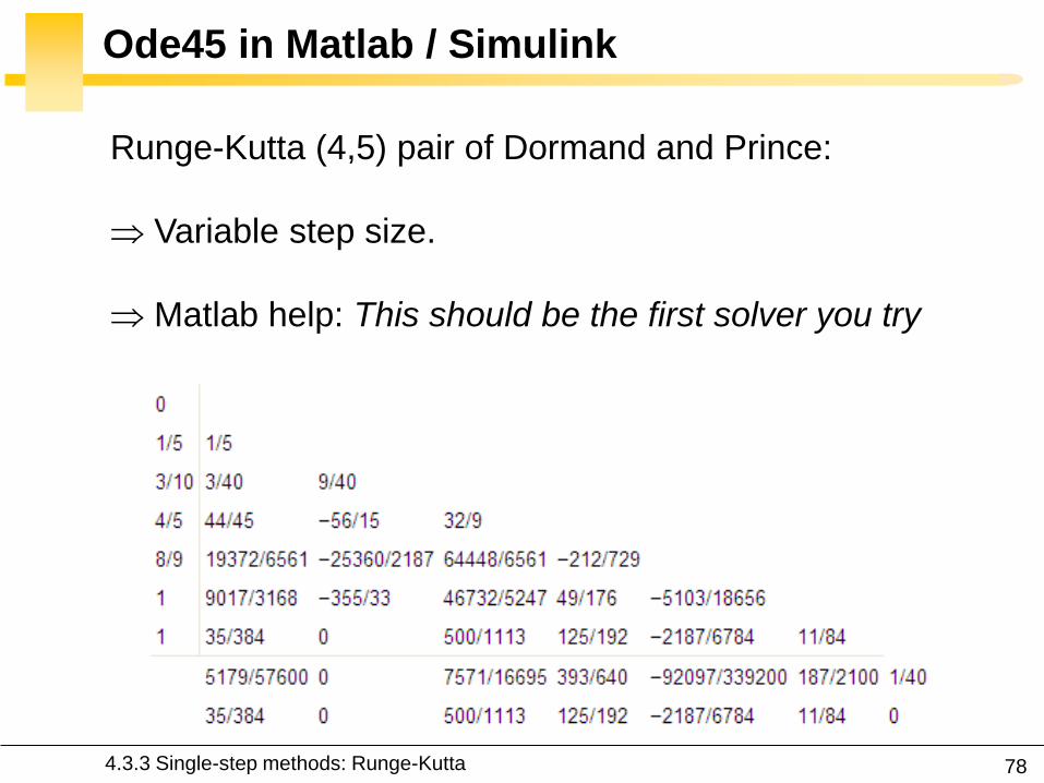
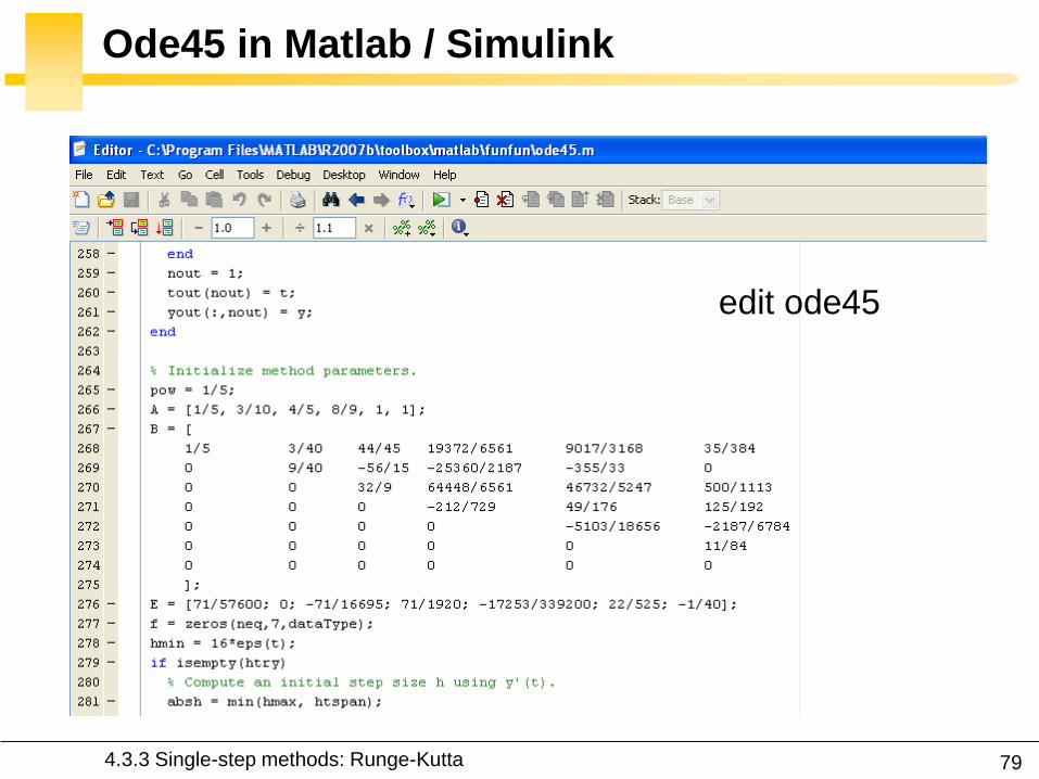
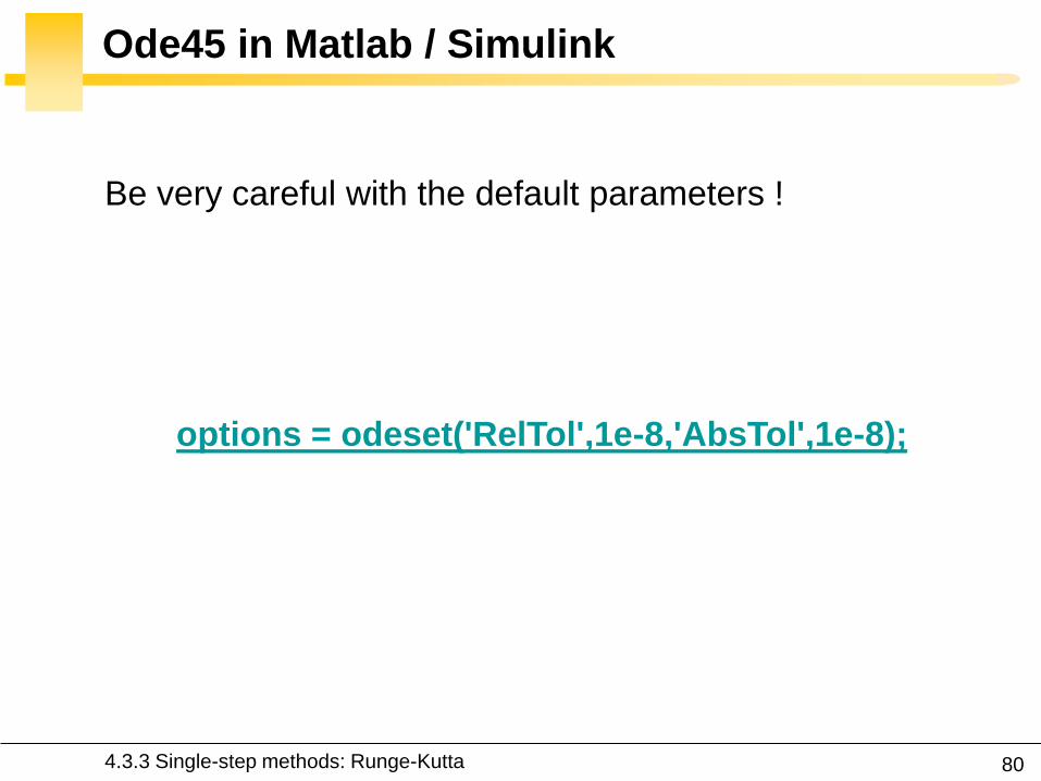
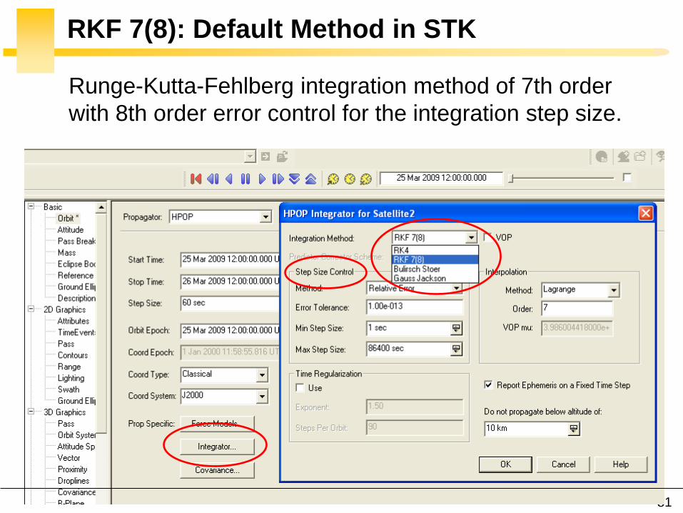
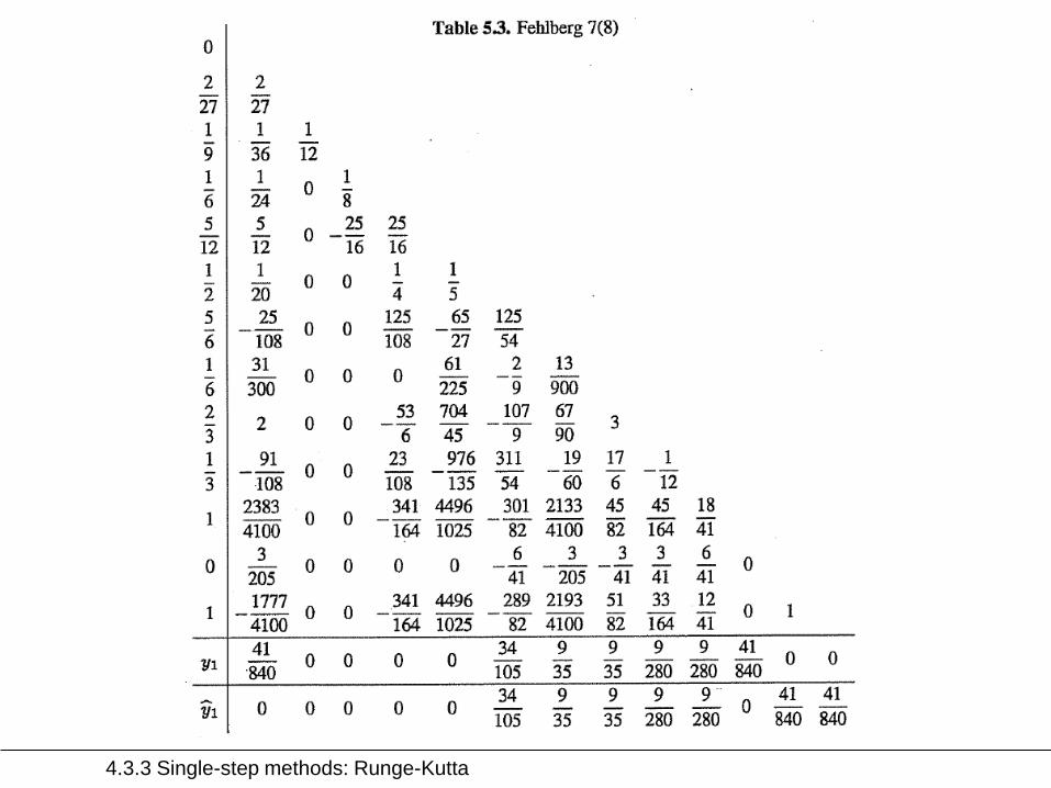
433 Single-step methods Runge-Kutta
83
Multi-Step Methods (Predictor-Corrector)
They estimate the state over time using previously
determined back values of the solution
Unlike RK methods they only perform one evaluation for
each step forward but they usually have a predictor and a
corrector formula
Adams() ndash Bashforth - Moulton Gauss - Jackson
() The first with Le Verrier to predict the existence and position of Neptune
434 Multi-step methods
84
Multi-Step Methods Principle
( ) ( )t f tu u1
1( ) ( ) ( ) n
n
t
n nt
t t f t dt
u u u
unknown
Replace it by a
polynomial that
interpolates the
previous values Four function values
interpolated by a
third-order polynomial
t
u
434 Multi-step methods
85
Multi-Step Methods Initiation
with ( ) ( )t f tu u 0 0( )t u u
What is the inherent problem
t
u
434 Multi-step methods
86
Multi-Step Methods Initiation
Because these methods require back values they are not
self-starting
One may for instance use of a single-step method to
compute the first four values
434 Multi-step methods
87
Gauss-Jackson in STK
One of the most recommendable fixed-stepsize multistep
methods for orbit computations
88
Integrator Selection
435 Integrator and step size selection
Montenbruck and Gill
Satellite orbits Springer
2000
89
Integrator Selection
Pros
Very fast
Cons
Special starting procedure
Fixed time steps
Error control
Pros
Plug and play
Error control
Cons
Slower
Multi-step Single step
435 Integrator and step size selection
90
Why is the Step Size So Critical
Theoretical arguments
1 The accuracy and the stability of the algorithm are
directly related to the step size
2 Nonlinear equations of motion
Data for Landsat 4 and 6 in circular orbits around 800km
indicates that a one-minute step size yields about 47m
error
A three-minute step size produces about a 900m error
435 Integrator and step size selection
91
Why is the Step Size So Critical
More practical arguments
1 The computation time is directly related to the
step size
2 The particular choice of step size depends on the
most rapidly varying component in the disturbing
functions (eg 50 x 50 gravity field)
435 Integrator and step size selection
92
Appropriate Step Size
The problem of determining an appropriate step size is a
challenge in any numerical process
Fixed step size (rule of thumb for standard
applications)
But an algorithm with variable step size is really
helpful The step size is chosen in such a way that
each step contributes uniformly to the total integration
error
100
orbitTt
435 Integrator and step size selection
93
Three Examples XMM OUFTI-1 ISS
Can you plot the step size vs true anomaly
435 Integrator and step size selection
94
XMM Report in STK
435 Integrator and step size selection
95
XMM (e~08)
0 50 100 150 200 250 300 350 4000
1000
2000
3000
4000
5000
6000
True anomaly (deg)
Ste
p s
ize
(s)
435 Integrator and step size selection
96
ISS(e~0)
435 Integrator and step size selection
0 50 100 150 200 250 300 350 40030
35
40
45
50
55
60
65
70
True anomaly (deg)
Ste
p s
ize
(s)
97
ldquoDifficultrdquo Orbits
Automatic time step is especially nice on highly eccentric
orbits (Molniya XMM) These orbits are best computed
using variable step sizes to maintain some given level of
accuracy
Without this variable step size we waste a lot of time near
apoapsis when the integration is taking too small a step
Likewise the integrator may not be using a small enough step
size at periapsis where the satellite is traveling fast
435 Integrator and step size selection
98
HPOP Propagator ISS Example
1 Earthrsquos oblateness only
2 Drag only
3 Sun and moon only
4 SRP only
5 All together
436 ISS example
99
Earthrsquos Oblateness Only Ω
HPOP
J2
2-body
436 ISS example
100
Earthrsquos Oblateness Only i Ω a
HPOP with central body (20 + WGS84_EGM96)
(without dragSRPSun and Moon)
436 ISS example
101
Drag Only i Ω a
HPOP with drag ndash Harris Priester
(without oblatenessSRPSun and Moon)
436 ISS example
102
Drag Relationship with Eclipses
103
SRP Only i Ω a
HPOP with SRP
(without oblatenessdragSun and Moon)
436 ISS example
104
SRP Relationship with Eclipses
105
All Perturbations Together
436 ISS example
106
4 Non-Keplerian Motion
2
2
(1 )
sin
sin 1 cos
a e
N
i e
44 Geostationary satellites
107
Practical Example GEO Satellites
Nice illustration of
1 Perturbations of the 2-body problem
2 Secular and periodic contributions
3 Accuracy required by practical applications
4 The need for orbit correction and thrust forces
And it is a real-life example (telecommunications
meteorology)
44 GEO satellites
108
Three Main Perturbations for GEO Satellites
44 GEO satellites
1 Non-spherical Earth
2 SRP
3 Sun and Moon
109
Station Keeping of GEO Satellites
The effect of the perturbations is to cause the spacecraft
to drift away from its nominal station If the drift was
allowed to build up unchecked the spacecraft could
become useless
A station-keeping box is defined by a longitude and a
maximum authorized distance for satellite excursions in
longitude and latitude
For instance TC2 -8ordm plusmn 007ordm EW plusmn 005ordm NS
44 GEO satellites
110
East-West and North-South Drift
44 GEO satellites
NS drift
EW drift
What are the perturbations generating these drifts
111
East-West Drift
44 GEO satellites
A GEO satellite drifts in longitude due to the influence of
two main perturbations
1 The elliptic nature of the Earthrsquos equatorial cross-
section J22 (and not from the NS oblateness J2)
2
ΔV
ΔV vsat
vsat SRP
112
East-West Drift due to Equatorial Ellipticity
44 GEO satellites
113
East-West Drift due to Equatorial Ellipticity
44 GEO satellites
114
East-West Drift HPOP (20) vs HPOP (22)
44 GEO satellites
115
East-West Drift Stable Equilibirum
HPOP with 22
(without Sun and moonSRPdrag)
116
East-West Drift Stable Equilibirum
HPOP with 22
(without Sun and moonSRPdrag)
117
East-West Drift Stable Equilibirum
HPOP with 22
(without Sun and moonSRPdrag)
118
North-South Drift
The perturbations caused by the Sun and the Moon are
predominantly out-of-plane effects causing a change in
the inclination and in the right ascension of the orbit
ascending node
Similar effects on the orbit to those of the Earthrsquos
oblateness (but here with respect to the ecliptic)
A GEO satellite therefore drifts in latitude with a
fundamental period equal to the orbit period
119
North-South Drift
Period
HPOP with Sun and Moon
(without oblatenessSRPdrag)
120
North-South Drift
Period
HPOP with Sun and Moon
(without oblatenessSRPdrag)
121
Thrust Forces for Stationkeeping
GEO spacecraft require continual stationkeeping to stay
within the authorized box using onboard thrusters
44 GEO satellites
122
42 ANALYTIC TREATMENT
421 Variation of parameters
422 Non-spherical Earth
423 J2 propagator in STK
424 Atmospheric drag
425 Third-body perturbations
426 SGP4 propagator in STK
427 Solar radiation pressure
4 Non-Keplerian Motion
43 NUMERICAL METHODS
431 Orbit prediction
432 Numerical integration
433 Single-step methods Runge-Kutta
434 Multi-step methods
435 Integrator and step size selection
436 ISS example
44 GEOSTATIONARY SATELLITES
Gaeumltan Kerschen
Space Structures amp
Systems Lab (S3L)
4B Non-Keplerian Motion
Astrodynamics (AERO0024)
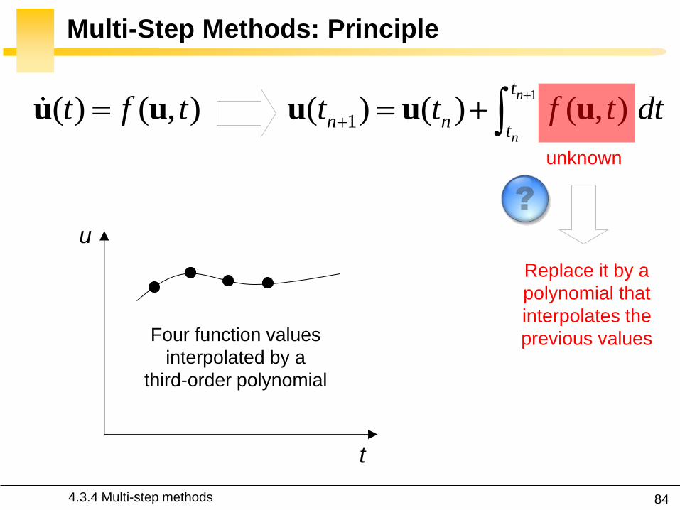
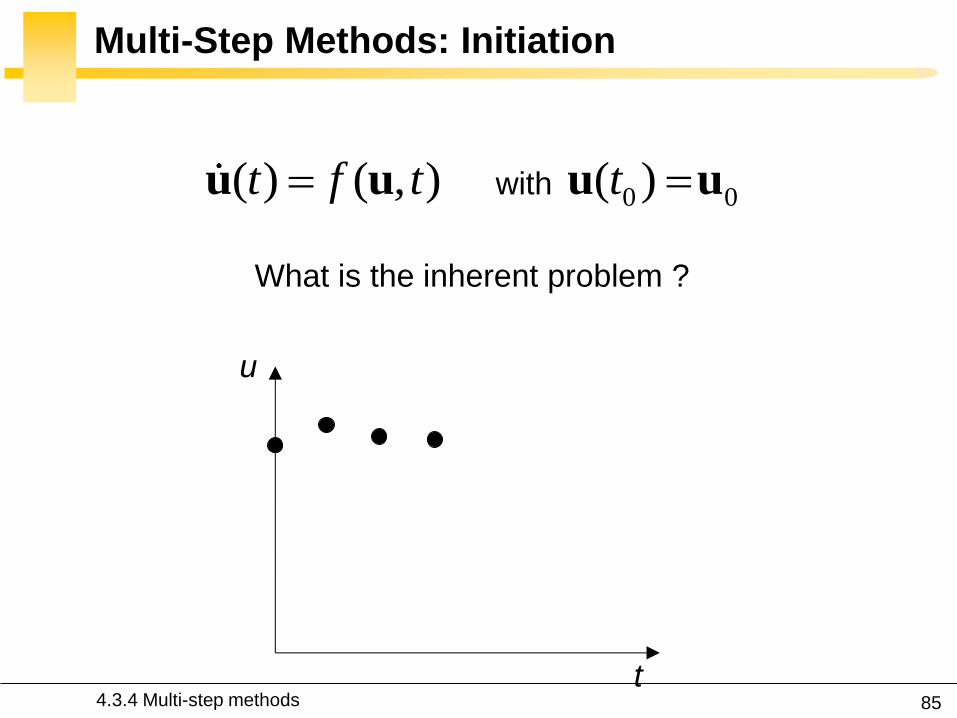
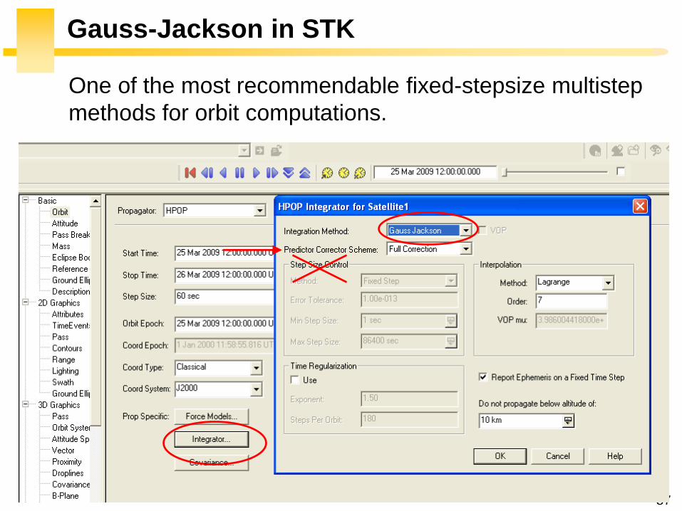
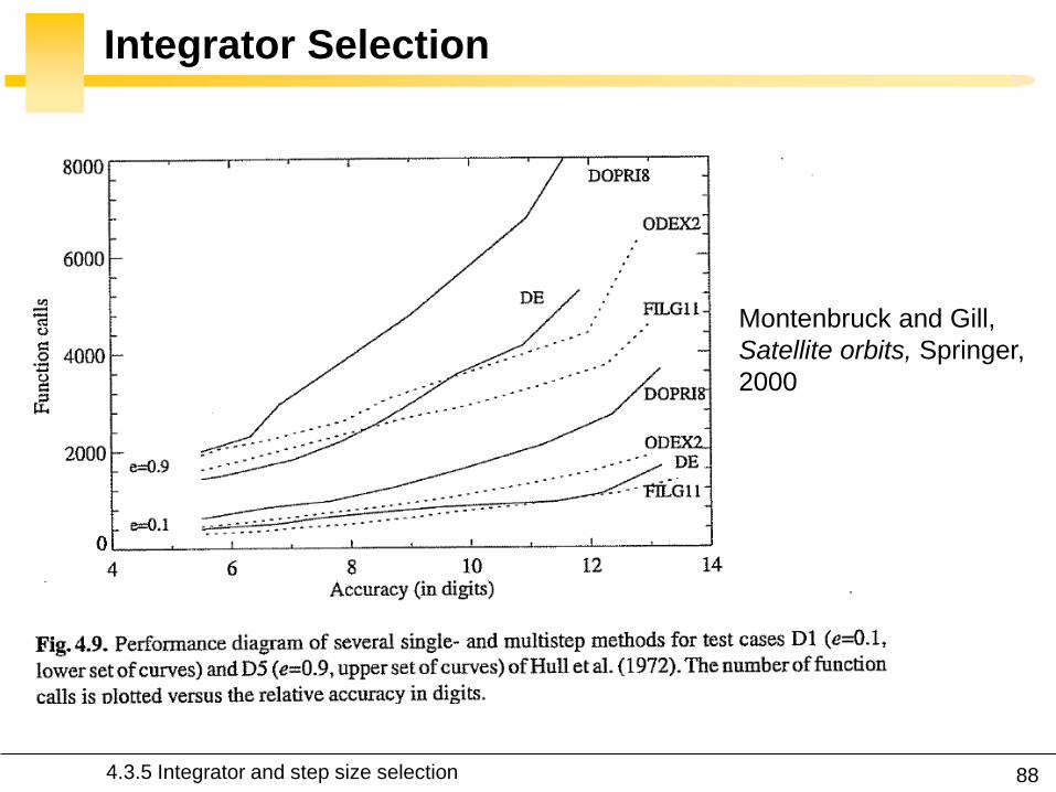
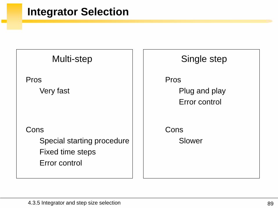
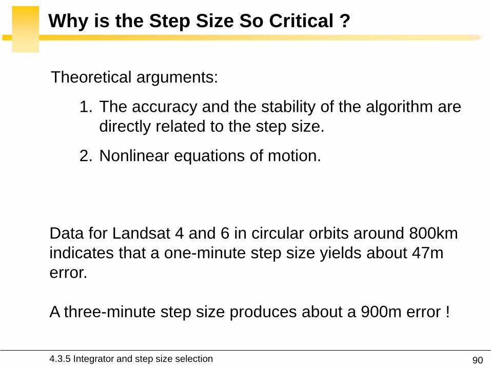
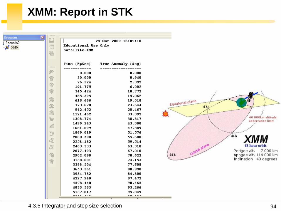
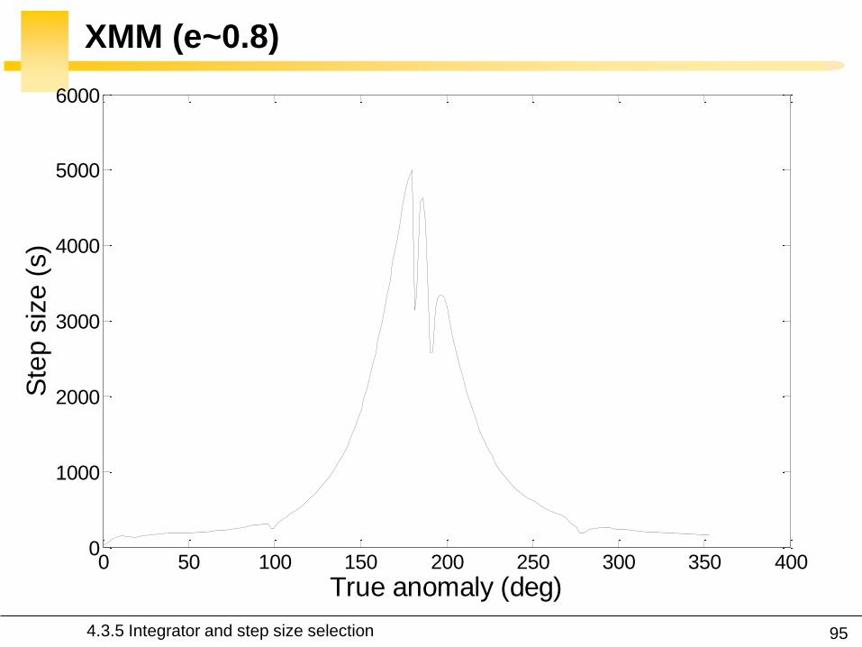
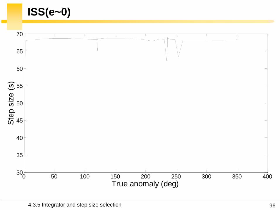
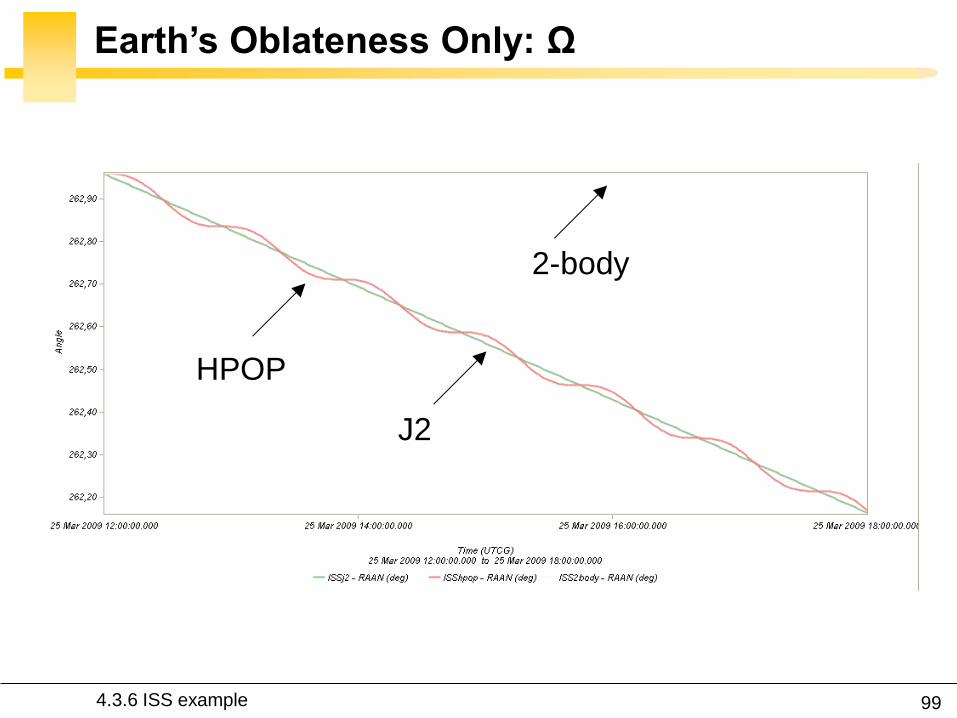
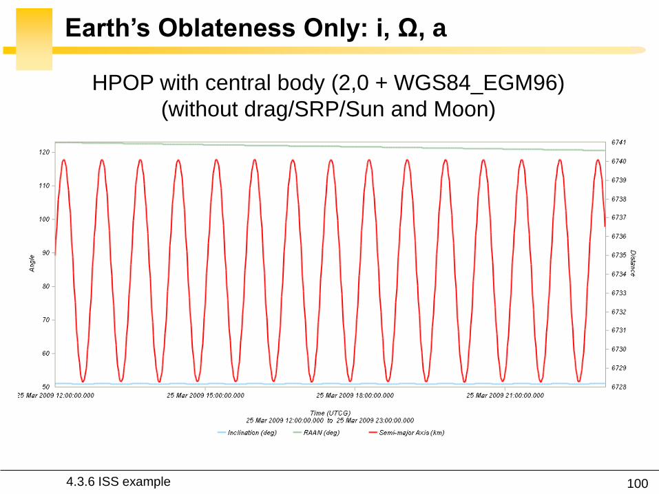
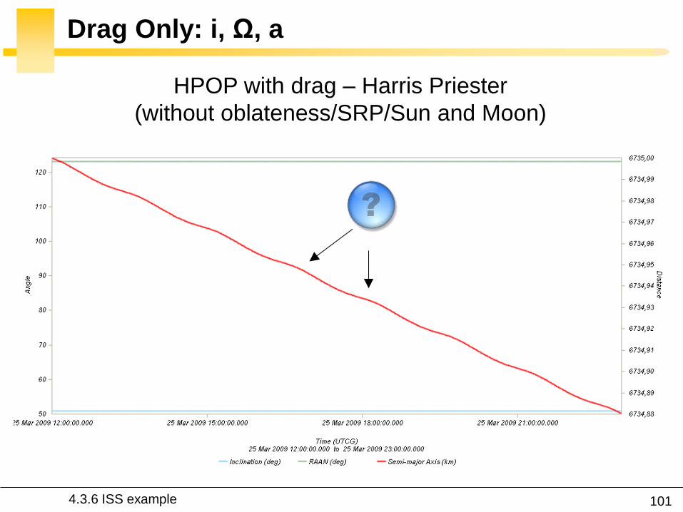
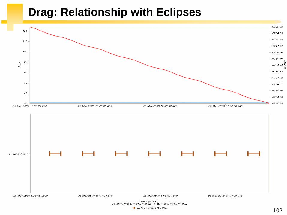
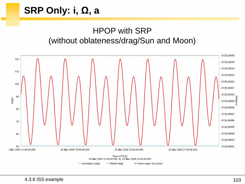
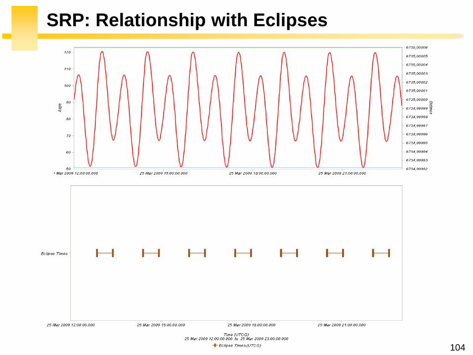
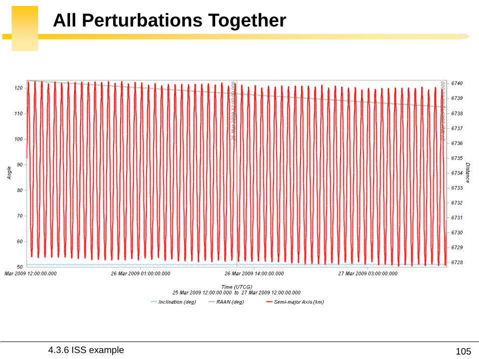
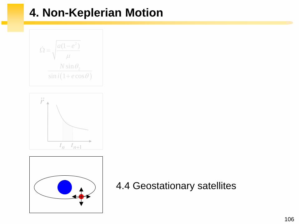
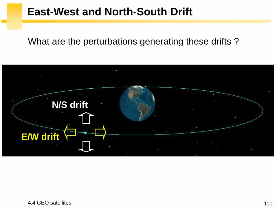
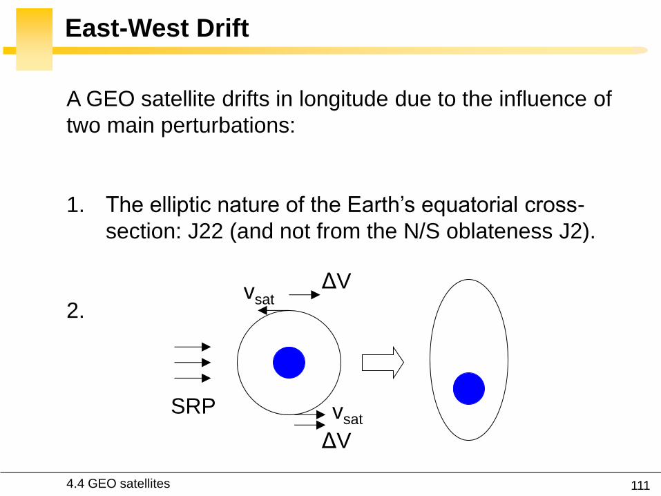
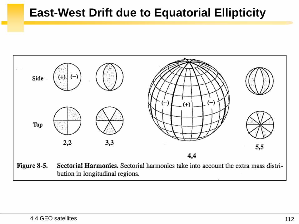
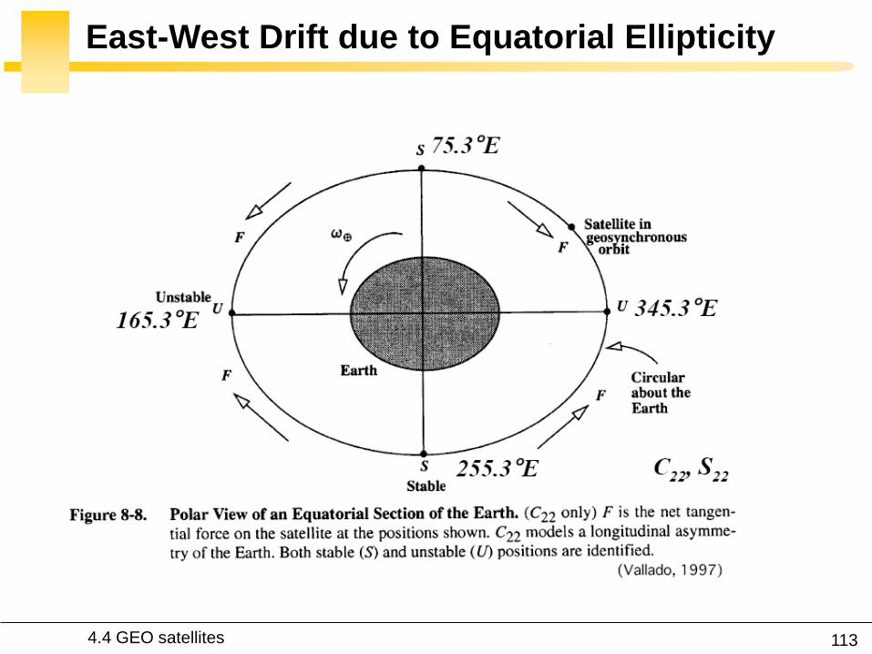
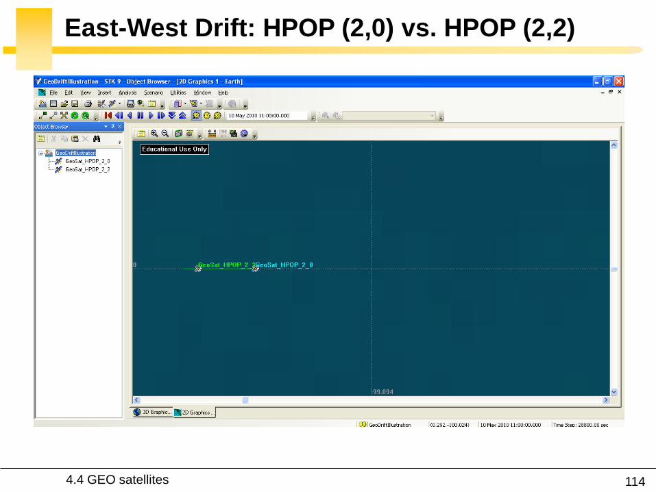
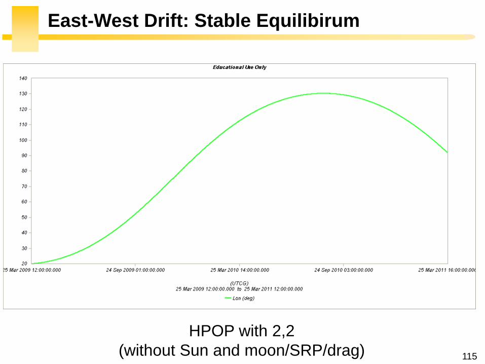
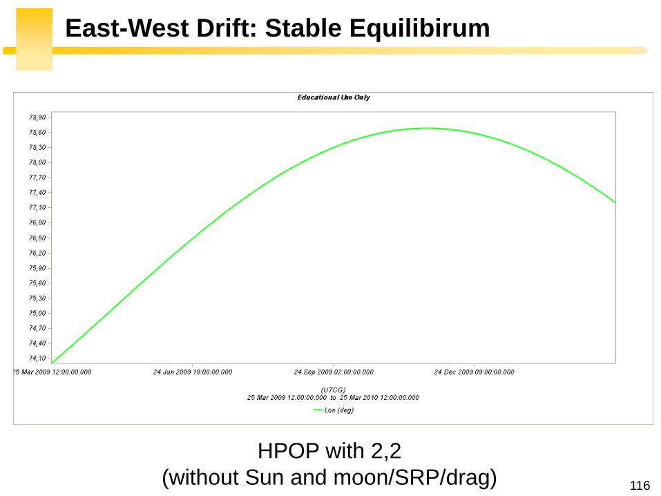
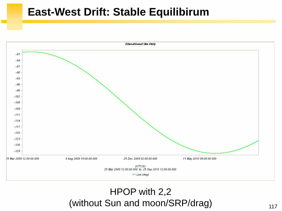
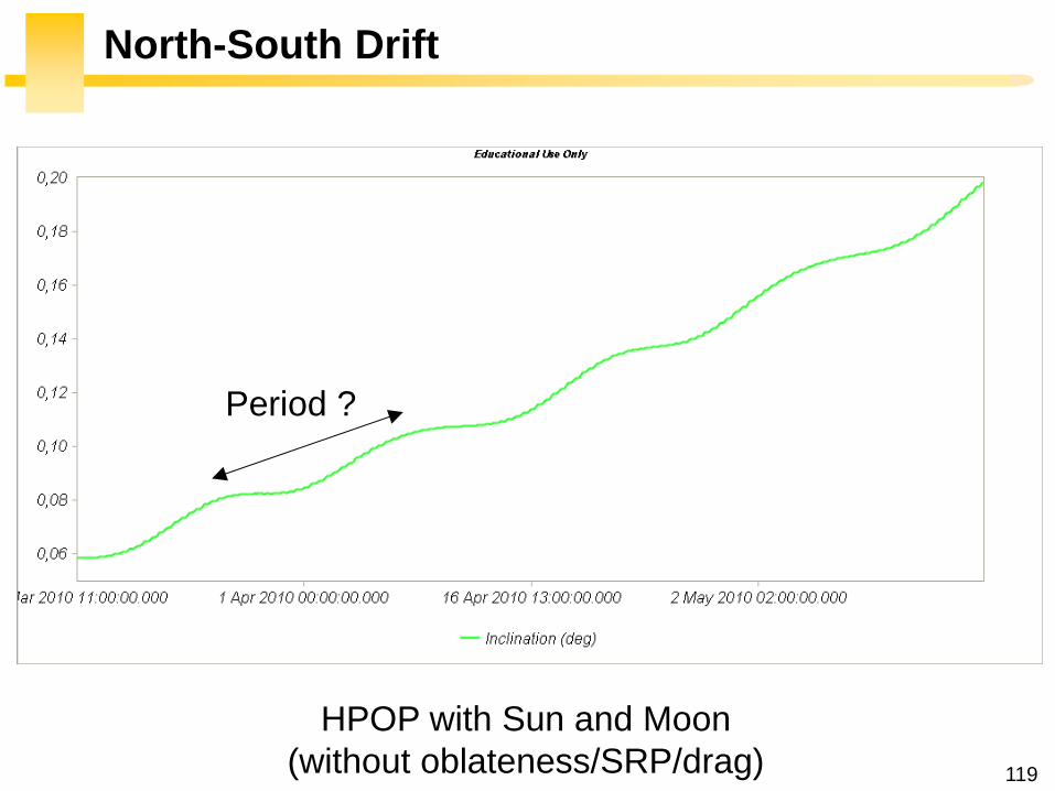
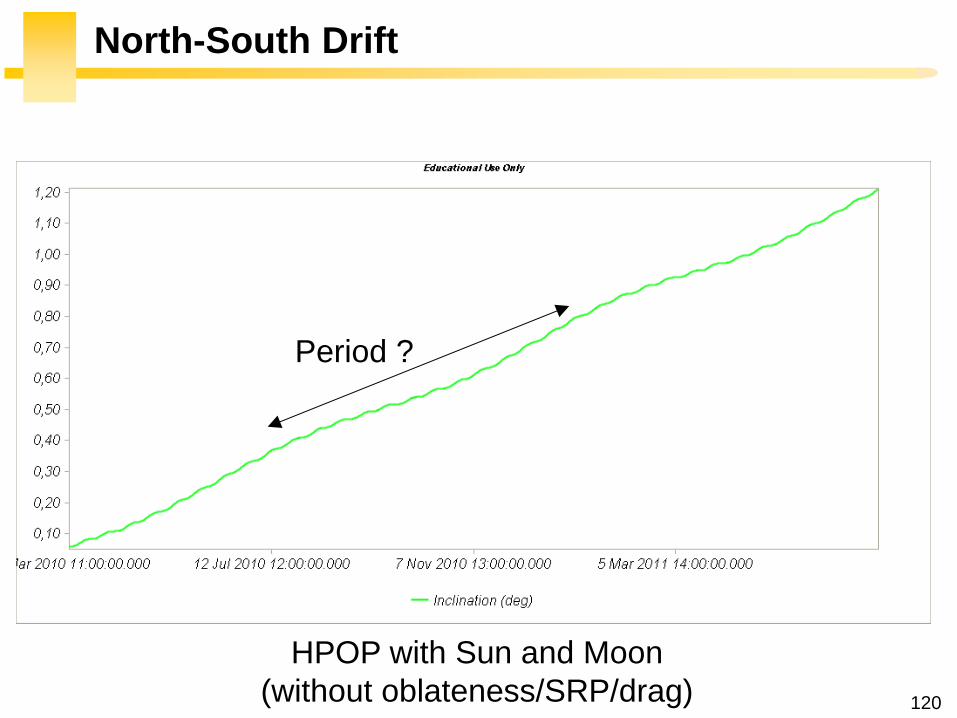
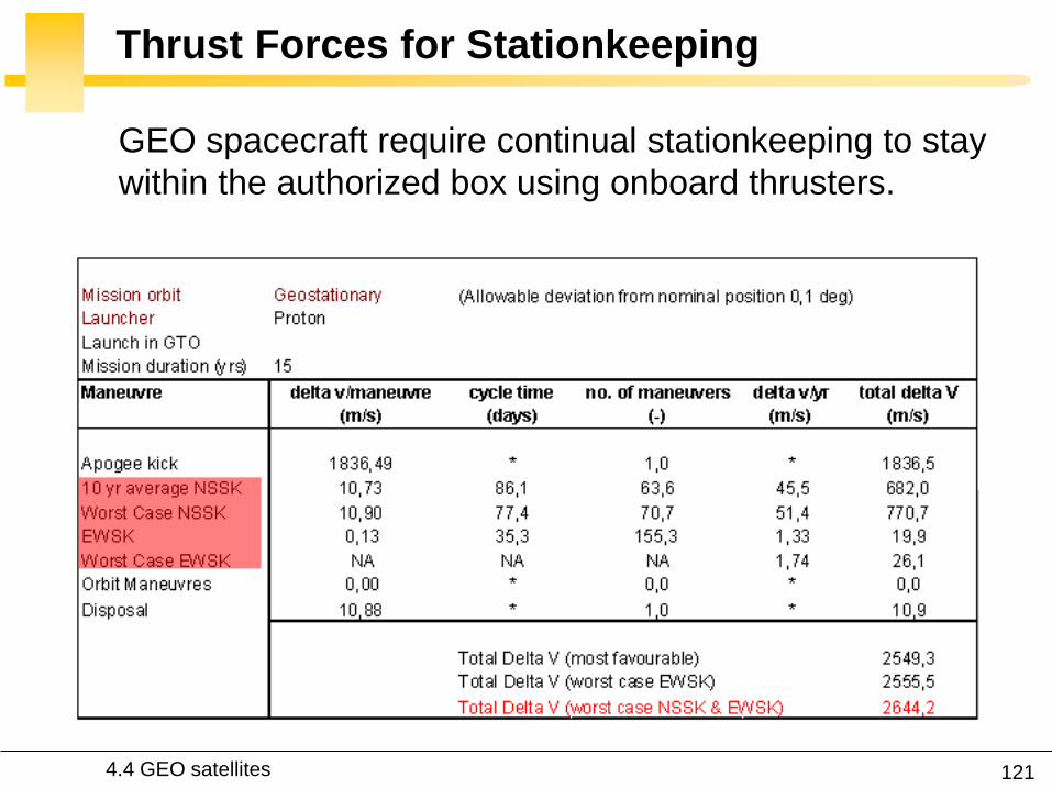
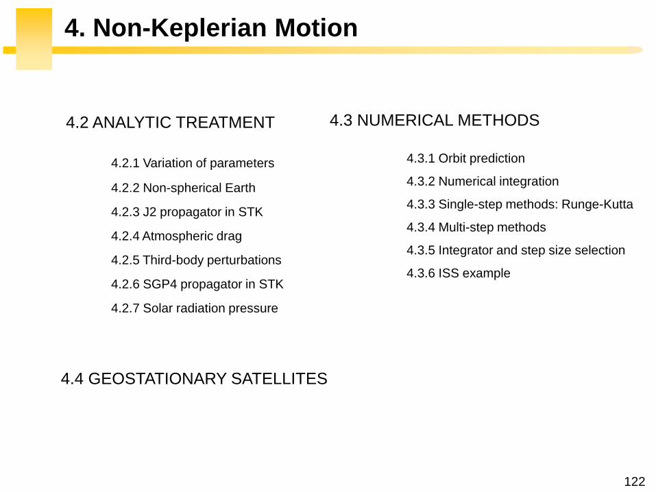
Gaeumltan Kerschen
Space Structures amp
Systems Lab (S3L)
4B Non-Keplerian Motion
Astrodynamics (AERO0024)