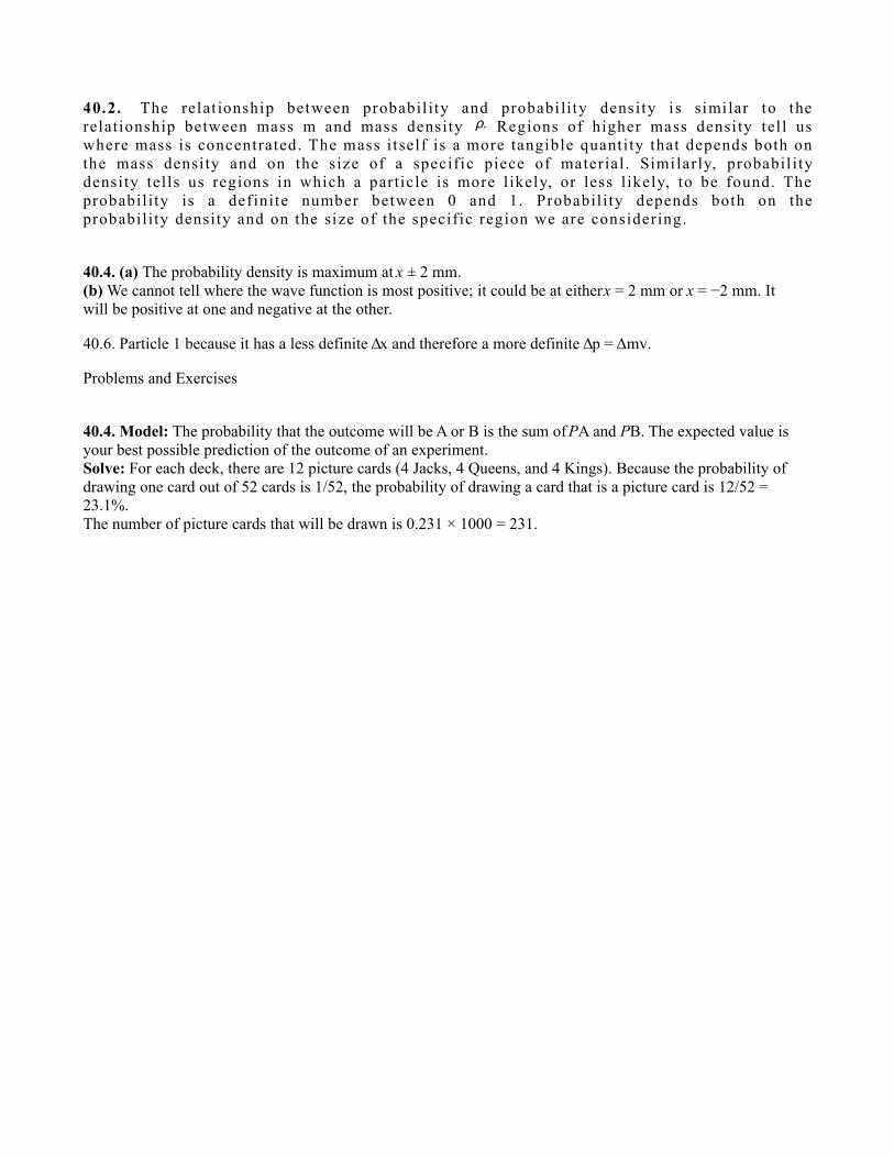
40.2. The relat ionship between probabil ity and probabi li ty density i s simi lar to the relationship between mass m and mass density ρ. Regions of higher mass densi ty tel l us where mass is concentrated. The mass i tself is a more tangible quantity that depends both on the mass densi ty and on the size of a specific piece of material . Simi larly, probabil i ty density tells us regions in which a particle is more l ikely, or less l ikely, to be found. The probabil i ty is a definite number between 0 and 1. Probabil i ty depends both on the probabil i ty density and on the size of the specific region we are considering.

40.4. (a) The probability density is maximum at x ± 2 mm.(b) We cannot tell where the wave function is most positive; it could be at either x = 2 mm or x = −2 mm. Itwill be positive at one and negative at the other.

40.6. Particle 1 because it has a less definite Δx and therefore a more definite Δp = Δmv.

Problems and Exercises

40.4. Model: The probability that the outcome will be A or B is the sum of PA and PB. The expected value isyour best possible prediction of the outcome of an experiment.Solve: For each deck, there are 12 picture cards (4 Jacks, 4 Queens, and 4 Kings). Because the probability ofdrawing one card out of 52 cards is 1/52, the probability of drawing a card that is a picture card is 12/52 = 23.1%.The number of picture cards that will be drawn is 0.231 × 1000 = 231.

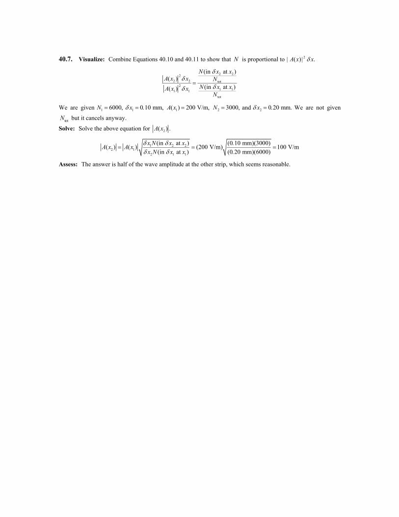
40.7. Visualize: Combine Equations 40.10 and 40.11 to show that N is proportional to 2( ) .A x xδ| |

2 222 2 tot

21 11 1

tot

(in at )( )

(in at )( )

N x xA x x N

N x xA x xN

δδ

δδ=

We are given 1 6000,N = 1 0 10 mm,xδ = . 1( ) 200 V m,A x = / 2 3000,N = and 2 0 20 mm.xδ = . We are not given

Ntot but it cancels anyway.

Solve: Solve the above equation for 2( ) .A x

1 2 22 1

2 1 1

(in at ) (0 10 mm)(3000)( ) ( ) (200 V m) 100 V m(in at ) (0 20 mm)(6000)

x N x xA x A xx N x x

δ δδ δ

.= = / = /

.

Assess: The answer is half of the wave amplitude at the other strip, which seems reasonable.

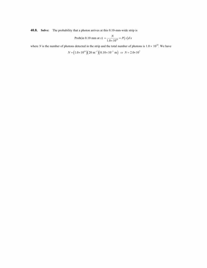
40.8. Solve: The probability that a photon arrives at this 0.10-mm-wide strip is

Prob(in 0.10 mm at x) ( )101.0 10N P x xδ= =×

where N is the number of photons detected in the strip and the total number of photons is 1.0 × 1010. We have

( )( )( )10 1 31.0 10 20 m 0.10 10 mN − −= × × ⇒ N = 2.0×107

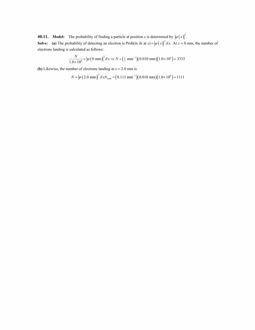
40.11. Model: The probability of finding a particle at position x is determined by ( ) 2.xψ

Solve: (a) The probability of detecting an electron is Prob(in δx at x) ( ) 2.x xψ δ= At x = 0 mm, the number of

electrons landing is calculated as follows:

( ) ( )( )( )2 1 6136 0 mm mm 0.010 mm 1.0 10 3333

1.0 10N x Nψ δ −= ⇒ = × =×

(b) Likewise, the number of electrons landing at x = 2.0 mm is

( ) ( )( )( )2 1 6total2.0 mm 0.111 mm 0.010 mm 1.0 10 1111N xNψ δ −= = × =

40.10. Solve: ( ) 2x xψ δ is a probability, which is dimensionless. The units of xδ are m, so the units of

( ) 2xψ are m−1 and thus the units of ψ are m−1/2.

40.14. Model: The probability of finding a particle is determined by the probability density ( ) ( ) 2P x xψ= .

Solve: (a) The normalization condition for a wave function: ( ) 2x dxψ

∞

−∞

=∫ area under the curve = 1. In the

present case, the area under the ( ) 2xψ -versus-x graph is 2 nm.a Hence, 11

2 nm .a −= (b) Each point on the ψ (x) graph is the square root of the corresponding point on the |ψ(x)|2 graph. Where the |ψ (x)|2 graph has dropped to 1/2 its maximum value at x = 1 nm, the ψ (x) graph will have dropped only to 1/ 2 0.707= of its maximum value. Thus the graph shape is convex upward. Since a = 1

2 nm–1, the peak value

of ψ (x) is 1/ 21/ 2 nma −= = 0.707 nm–1/2. The graph is shown below. The negative of this graph, curving downward, would also be an acceptable wave function.

(c) The probability of the electron being located in the interval 1.0 ≤ x ≤ 2.0 nm is

1

Prob(1.0 nm 2.0 nm) area under the curve between 1.0 nm and 2.0 nm1 (0.50 nm )(1.0 nm)(2.0 nm – 1.0 nm) 0.1252 2 4

xa −

≤ ≤ =

⎛ ⎞= = =⎜ ⎟⎝ ⎠

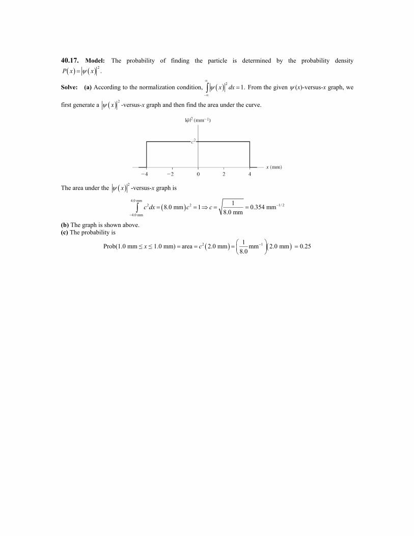
40.17. Model: The probability of finding the particle is determined by the probability density

( ) ( ) 2.P x xψ=

Solve: (a) According to the normalization condition, ( ) 21.x dxψ

∞

−∞

=∫ From the given ψ (x)-versus-x graph, we

first generate a ( ) 2xψ -versus-x graph and then find the area under the curve.

The area under the ( ) 2xψ -versus-x graph is

( )4.0 mm

2 2 1/ 2

4.0 mm

18.0 mm 1 0.354 mm8.0 mm

c dx c c −

−

= = ⇒ = =∫

(b) The graph is shown above. (c) The probability is

Prob(1.0 mm ≤ x ≤ 1.0 mm) = ( ) ( )2 11area 2.0 mm mm 2.0 mm8.0

c −⎛ ⎞= = ⎜ ⎟⎝ ⎠

= 0.25

40.19. Model: A radio-frequency pulse is an electromagnetic wave packet, hence it must satisfy the relationship Δ f Δ t ≈ 1. Solve: The waves that must be superimposed to create the pulse of smallest duration span the frequency range f – Δ f /2 ≤ f ≤ f + Δ f /2 . Because Δ f = 120 MHz – 80 MHz = 40 MHz, f = 100 MHz. Using Equation 40.20,

81 1 2.5 10 s 25 ns40 MHz

tf

−Δ ≈ = = × =Δ

Thus, a radio wave centered at 100 MHz and having a frequency span 80 MHz to 120 MHz can be used to create a wave of duration 25 ns.

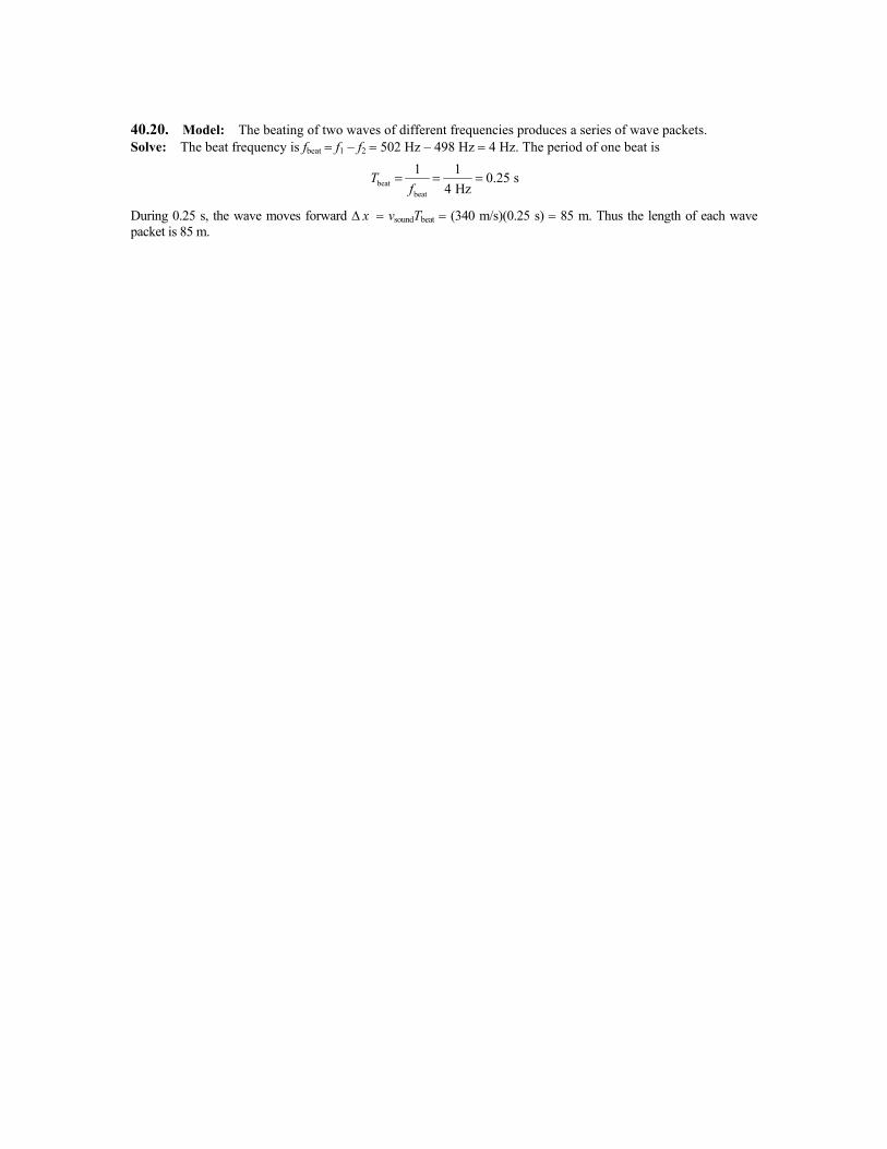
40.20. Model: The beating of two waves of different frequencies produces a series of wave packets. Solve: The beat frequency is fbeat = f1 – f2 = 502 Hz – 498 Hz = 4 Hz. The period of one beat is

beatbeat

1 1 0.25 s4 Hz

Tf

= = =

During 0.25 s, the wave moves forward ∆ x = vsoundTbeat = (340 m/s)(0.25 s) = 85 m. Thus the length of each wave packet is 85 m.

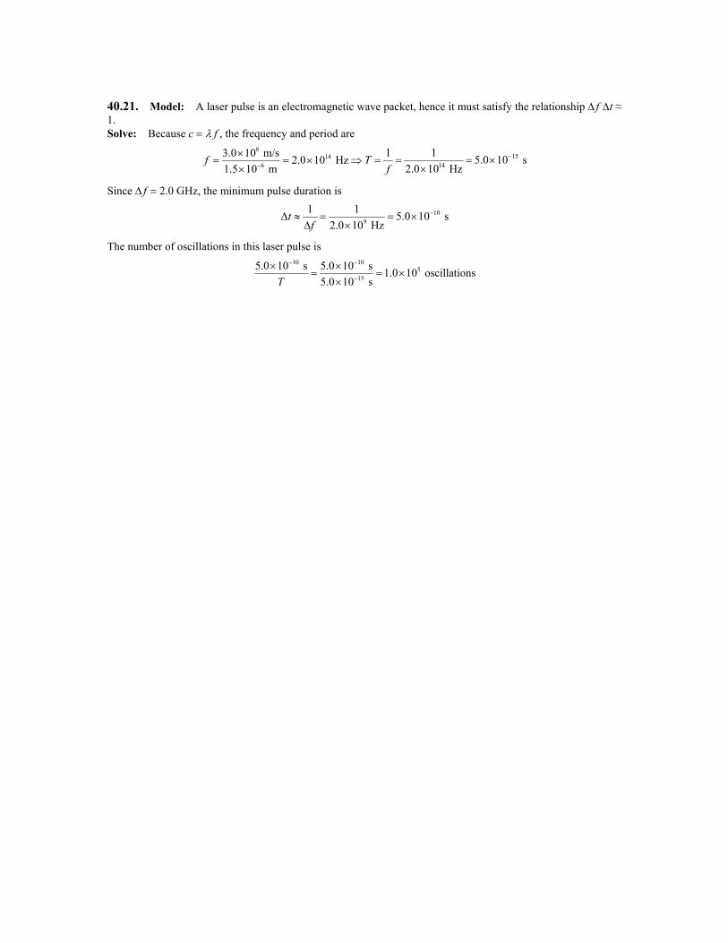
40.21. Model: A laser pulse is an electromagnetic wave packet, hence it must satisfy the relationship Δ f Δt ≈ 1. Solve: Because c = λ f , the frequency and period are

814

6

3.0 10 m/s 2.0 10 Hz1.5 10 m

f −

×= = × ⇒

×15

14

1 1 5.0 10 s2.0 10 Hz

Tf

−= = = ××

Since Δ f = 2.0 GHz, the minimum pulse duration is

109

1 1 5.0 10 s2.0 10 Hz

tf

−Δ ≈ = = ×Δ ×

The number of oscillations in this laser pulse is 10 10

515

5.0 10 s 5.0 10 s 1.0 10 oscillations5.0 10 sT

− −

−

× ×= = ×

×

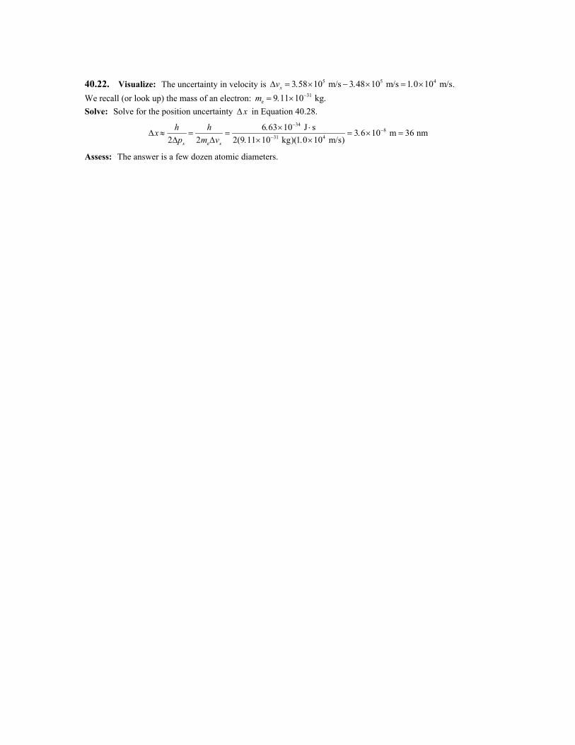
40.22. Visualize: The uncertainty in velocity is 5 5 43 58 10 m s 3 48 10 m s 1 0 10 m sxvΔ = . × / − . × / = . × / . We recall (or look up) the mass of an electron: 31

e 9 11 10 kg.m −= . × Solve: Solve for the position uncertainty xΔ in Equation 40.28.

348

31 4e

6 63 10 J s 3 6 10 m 36 nm2 2 2(9 11 10 kg)(1 0 10 m s)x x

h hxp m v

−−

−

. × ⋅Δ ≈ = = = . × =

Δ Δ . × . × /

Assess: The answer is a few dozen atomic diameters.

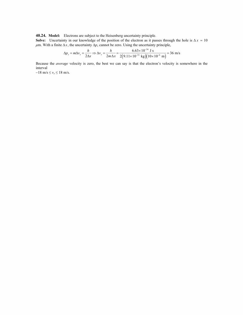
40.24. Model: Electrons are subject to the Heisenberg uncertainty principle. Solve: Uncertainty in our knowledge of the position of the electron as it passes through the hole is Δ x = 10 μm. With a finite Δx , the uncertainty Δpx cannot be zero. Using the uncertainty principle,

( )( )34

31 6

6.63 10 J s 36 m/s2 2 2 9.11 10 kg 10 10 mx x x

h hp m v vx m x

−

− −

×Δ = Δ = ⇒ Δ = = =

Δ Δ × ×

Because the average velocity is zero, the best we can say is that the electron’s velocity is somewhere in the interval −18 m/s ≤ vx ≤ 18 m/s.

40.25. Model: Protons are subject to the Heisenberg uncertainty principle. Solve: We know the proton is somewhere within the nucleus, so the uncertainty in our knowledge of its position is at most Δx = L = 4.0 fm. With a finite Δ x , the uncertainty Δpx is given by the uncertainty principle:

( )( )34

727 15

/2 6.63 10 J s 5.0 10 m/s2 2 1.67 10 kg 4.0 10 mx x x

h hp m v vx mL

−

− −

×Δ = Δ = ⇒ Δ = = = ×

Δ × ×

Because the average velocity is zero, the best we can say is that the proton’s velocity is somewhere in the range −2.5 × 107 m/s to 2.5 × 107 m/s. Thus the smallest range of speeds is 0 to 2.5 × 107 m/s.

40.29. Model: The radio-wave pulses are wave packets, so each packet satisfies the relationship Δ f Δt ≈ 1. Visualize: Please refer to Figure P40.29. Solve: Because the frequency bandwidth is Δ f = 200 kHz, the shortest possible pulse width is

61 1 5 10 s200 kHz

tf

−Δ ≈ = = ×Δ

This means the time period of the pulse train is T = 2Δt = 2(5 × 10−6 s) = 10 × 10−6 s

So, the frequency of the pulse train is 51 1.0 10 Hz.f T= = × That is, the maximum transmission rate is 51.0 10 pulses/s.×

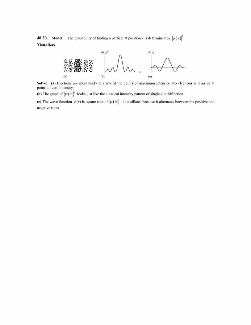
40.30. Model: The probability of finding a particle at position x is determined by ( ) 2.xψ

Visualize:

Solve: (a) Electrons are most likely to arrive at the points of maximum intensity. No electrons will arrive at points of zero intensity. (b) The graph of ( ) 2

xψ looks just like the classical intensity pattern of single-slit diffraction.

(c) The wave function ψ (x) is square root of ( ) 2.xψ It oscillates because it alternates between the positive and

negative roots.

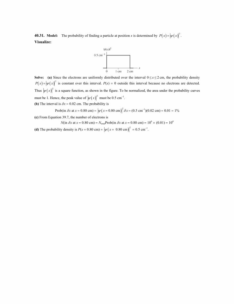
40.31. Model: The probability of finding a particle at position x is determined by ( ) ( ) 2.P x xψ=

Visualize:

Solve: (a) Since the electrons are uniformly distributed over the interval 0 ≤ x ≤ 2 cm, the probability density

( ) ( ) 2P x xψ= is constant over this interval. P(x) = 0 outside this interval because no electrons are detected.

Thus ( ) 2xψ is a square function, as shown in the figure. To be normalized, the area under the probability curves

must be 1. Hence, the peak value of ( ) 2xψ must be 0.5 cm−1.

(b) The interval is δx = 0.02 cm. The probability is

Prob(in δx at x = 0.80 cm) = ( ) 20.80 cmx xψ δ= = (0.5 cm−1)(0.02 cm) = 0.01 = 1%

(c) From Equation 39.7, the number of electrons is N(in δx at x = 0.80 cm) = NtotalProb(in δx at x = 0.80 cm) = 106 × (0.01) = 104

(d) The probability density is P(x = 0.80 cm) = ( ) 20.80 cmxψ = = 0.5 cm−1.

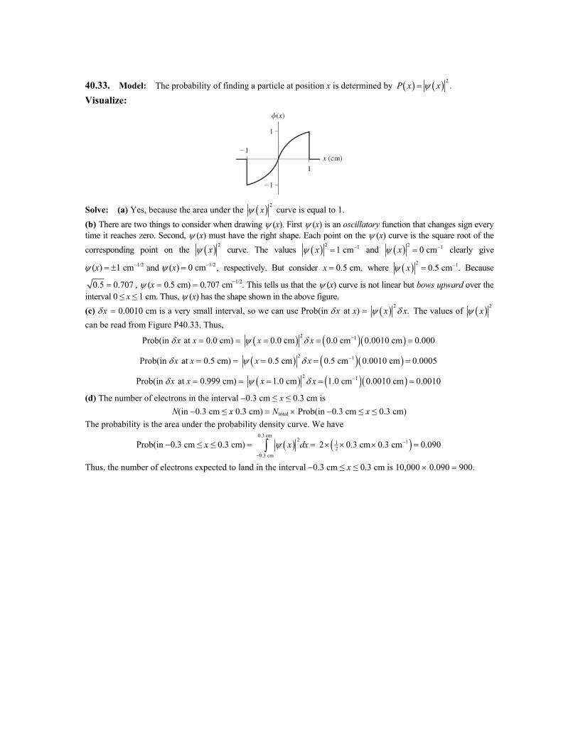
40.33. Model: The probability of finding a particle at position x is determined by ( ) ( ) 2.P x xψ=

Visualize:

Solve: (a) Yes, because the area under the ( ) 2xψ curve is equal to 1.

(b) There are two things to consider when drawing ψ (x). First ψ (x) is an oscillatory function that changes sign every time it reaches zero. Second, ψ (x) must have the right shape. Each point on the ψ (x) curve is the square root of the corresponding point on the ( ) 2

xψ curve. The values ( ) 2 11 cmxψ −= and ( ) 2 10 cmxψ −= clearly give 1/2( ) 1 cmxψ −= ± and 1/2( ) 0 cm ,xψ −= respectively. But consider 0.5 cm,x = where ( ) 2 10.5 cm .xψ −= Because

0.5 0.707= , ψ (x = 0.5 cm) = 0.707 cm−1/2. This tells us that the ψ (x) curve is not linear but bows upward over the interval 0 ≤ x ≤ 1 cm. Thus, ψ (x) has the shape shown in the above figure. (c) δx = 0.0010 cm is a very small interval, so we can use Prob(in δx at x) = ( ) 2

.x xψ δ The values of ( ) 2xψ

can be read from Figure P40.33. Thus,

Prob(in δx at x = 0.0 cm) = ( ) ( )( )2 10.0 cm 0.0 cm 0.0010 cm 0.000x xψ δ −= = =

Prob(in δx at x = 0.5 cm) = ( ) ( )( )2 10.5 cm 0.5 cm 0.0010 cm 0.0005x xψ δ −= = =

Prob(in δx at x = 0.999 cm) = ( ) ( )( )2 11.0 cm 1.0 cm 0.0010 cm 0.0010x xψ δ −= = =

(d) The number of electrons in the interval −0.3 cm ≤ x ≤ 0.3 cm is N(in −0.3 cm ≤ x 0.3 cm) = Ntotal × Prob(in −0.3 cm ≤ x ≤ 0.3 cm)

The probability is the area under the probability density curve. We have

Prob(in −0.3 cm ≤ x ≤ 0.3 cm) = ( )0.3 cm

2

0.3 cm

x dxψ−∫ = ( )11

22 0.3 cm 0.3 cm 0.090−× × × =

Thus, the number of electrons expected to land in the interval −0.3 cm ≤ x ≤ 0.3 cm is 10,000 × 0.090 = 900.

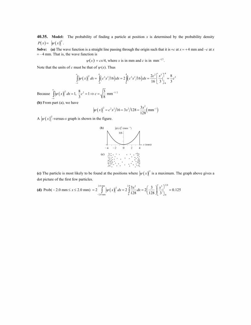
40.35. Model: The probability of finding a particle at position x is determined by the probability density

( )P x = ( ) 2xψ .

Solve: (a) The wave function is a straight line passing through the origin such that it is +c at x = +4 mm and –c at x = –4 mm. That is, the wave function is

ψ x( ) = cx/4, where x is in mm and c is in 1 2mm .−

Note that the units of c must be that of ψ (x). Thus

( ) ( ) ( )44 4 2 3

2 2 2 2 2 2

4 0 0

2 816 2 1616 3 3c xx dx c x dx c x dx cψ

∞

−∞ −

⎡ ⎤= = = =⎢ ⎥

⎣ ⎦∫ ∫ ∫

Because ( ) 2 2 1/ 28 31, 1 mm3 8

x dx c cψ∞

−

−∞

= = ⇒ =∫

(b) From part (a), we have

( ) ( )2

2 2 2 2 1316 3 128 mm128

xx c x xψ −= = =

A ( ) 2xψ -versus-x graph is shown in the figure.

(c) The particle is most likely to be found at the positions where ( ) 2xψ is a maximum. The graph above gives a

dot picture of the first few particles.

(d) ( )2.02.0 mm 2.0 2 3

2

2.0 mm 0 0

3 3Prob( 2.0 mm 2.0 mm) 2 2 2 0.125128 128 3

x xx x dx dxψ−

⎡ ⎤⎛ ⎞− ≤ ≤ = = = =⎢ ⎥⎜ ⎟⎝ ⎠ ⎣ ⎦

∫ ∫

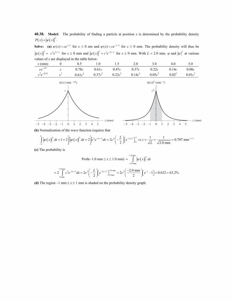
40.38. Model: The probability of finding a particle at position x is determined by the probability density

( ) ( ) 2.P x xψ=

Solve: (a) /( ) x Lx ceψ = for x ≤ 0 nm and /( ) x Lx ceψ −= for x ≥ 0 mm. The probability density will thus be

( ) 2xψ = 2 2 /x Lc e for x ≤ 0 mm and ( ) 2 2 2 /x Lx c eψ −= for x ≥ 0 mm. With L = 2.0 mm, ψ and 2ψ at various

values of x are displayed in the table below. x (mm) 0 0.5 1.0 1.5 2.0 3.0 4.0 5.0 ce−x/L c 0.78c 0.61c 0.47c 0.37c 0.22c 0.14c 0.08c

c2e−2x/L c2 0.61c2 0.37c2 0.22c2 0.14c2 0.05c2 0.022 0.01c2

(b) Normalization of the wave function requires that

( ) ( )2 2 2 2 / 2 2 1/ 2

00 0

1 11 2 2 2 0.707 mm2 2.0 mm

x L x LLx dx x dx c e dx c e cL

ψ ψ∞ ∞ ∞

∞− − −

−∞

⎛ ⎞ ⎡ ⎤= = = = − ⇒ = = =⎜ ⎟⎣ ⎦⎝ ⎠∫ ∫ ∫

(c) The probability is

Prob(−1.0 mm ≤ x ≤ 1.0 mm) ( )1.0 mm

2

1.0 mm

x dxψ−

= ∫

1.0 mm1.0 mm2 2 / 2 2 / 2 1

0 mm0 mm

2.0 mm2 2 2 1 0.632 63.2%2 2

x L x LLc e dx c e c e− − −−⎛ ⎞ ⎛ ⎞⎡ ⎤ ⎡ ⎤= = − = − = =⎜ ⎟ ⎜ ⎟⎣ ⎦ ⎣ ⎦⎝ ⎠ ⎝ ⎠∫

(d) The region –1 mm ≤ x ≤ 1 mm is shaded on the probability density graph.

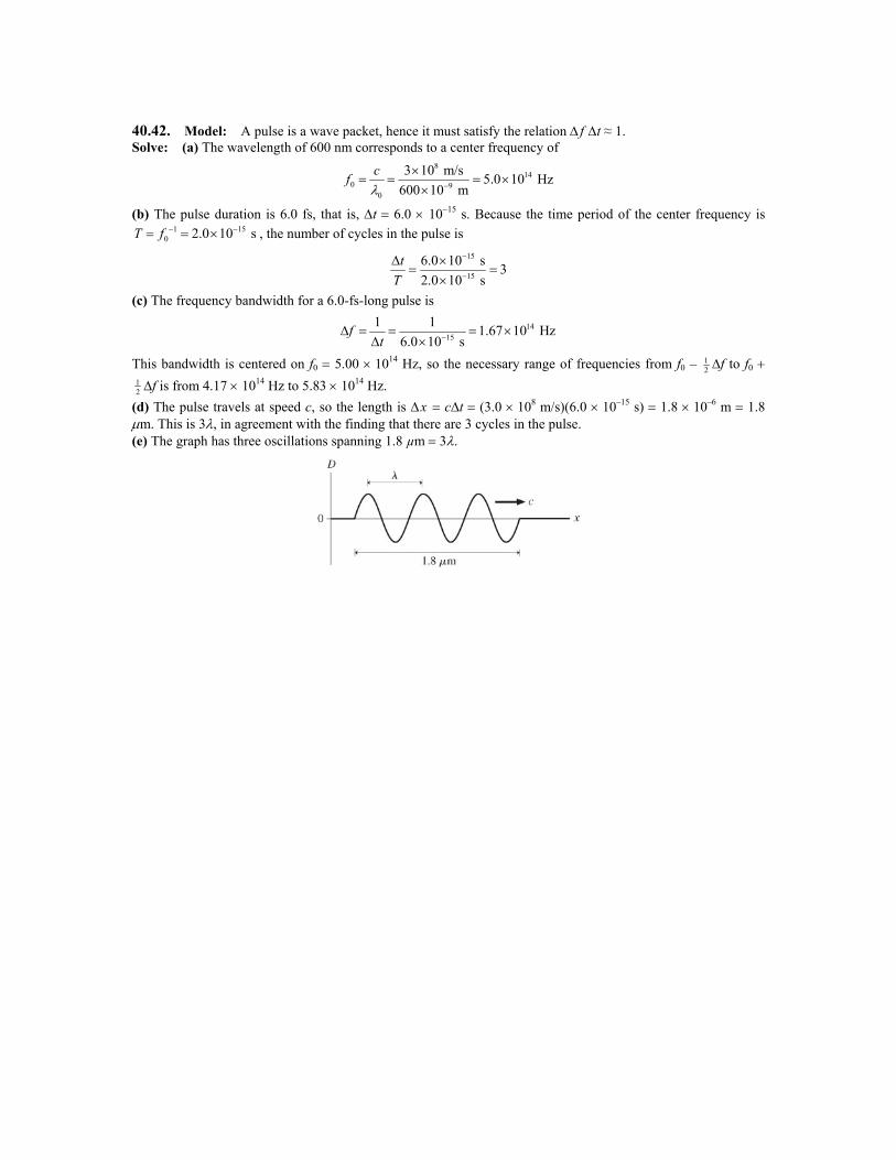
40.42. Model: A pulse is a wave packet, hence it must satisfy the relation Δ f Δt ≈ 1. Solve: (a) The wavelength of 600 nm corresponds to a center frequency of

814

0 90

3 10 m/s 5.0 10 Hz600 10 m

cfλ −

×= = = ×

×

(b) The pulse duration is 6.0 fs, that is, Δt = 6.0 × 10−15 s. Because the time period of the center frequency is 1 15

0 2.0 10 sT f − −= = × , the number of cycles in the pulse is 15

15

6.0 10 s 32.0 10 s

tT

−

−

Δ ×= =

×

(c) The frequency bandwidth for a 6.0-fs-long pulse is

1415

1 1 1.67 10 Hz6.0 10 s

ft −Δ = = = ×

Δ ×

This bandwidth is centered on f0 = 5.00 × 1014 Hz, so the necessary range of frequencies from f0 – 12 ∆f to f0 +

12 ∆f is from 4.17 × 1014 Hz to 5.83 × 1014 Hz.

(d) The pulse travels at speed c, so the length is ∆x = c∆t = (3.0 × 108 m/s)(6.0 × 10–15 s) = 1.8 × 10–6 m = 1.8 μm. This is 3λ, in agreement with the finding that there are 3 cycles in the pulse. (e) The graph has three oscillations spanning 1.8 µm = 3λ.

40.44. Model: A dust speck is a particle and is thus subject to the Heisenberg uncertainty principle. Solve: The uncertainty in our knowledge of the position of the dust speck is 10 m.x μΔ = The uncertainty in the dust speck’s momentum is

( )34

296

/ 2 6.63 10 J s 3.32 10 kg m/s2 10 10 mx

hpx

−−

−

×Δ = = = ×

Δ ×

Equivalently, the uncertainty in the dust particle velocity is 29

1316

3.32 10 kg m/s 3.32 10 m/s1.0 10 kg

xx

pvm

−−

−

Δ ×Δ = = = ×

×

The average velocity is 0 m/s, so the range of possible velocities is –1.66 × 10–13 m/s to +1.66 × 10–13 m/s. The particle could have a top speed of up to 1.66 × 10–13 m/s. The maximum kinetic energy the speck has is

( )( )22 16 13

42

1 1 1.0 10 kg 1.66 10 m/s2 21.4 10 J

K mv − −

−

= = × ×

= ×

To get out of the hole, the particle would have to acquire potential energy

( )( )( )16 2 6

22

1.0 10 kg 9.8 m/s 1.0 10 m

9.8 10 J

U mgh − −

−

= = × ×

= ×

The energy gain needed to get out of the hole is much larger than the available kinetic energy. The particle does not have anywhere near enough kinetic energy that it could, by any process, transform into potential energy and escape. Using K = mgh, the deepest hole from which the dust speck could have a good chance of escaping is

( )( )42

2716 2

1.4 10 J 1.4 10 m1.0 10 kg 9.8 m/s

Khmg

−−

−

×= = = ×

×

Assess: This is not a very deep hole.

40.47. Solve: (a) For a photon, E = hf which means ΔE = hΔ f . Assuming the photon is a wave packet, the relationship that is applicable to a wave packet Δ f Δt ≈ 1 becomes

1E thΔ⎛ ⎞Δ ≈ ⇒⎜ ⎟

⎝ ⎠ΔEΔt ≈ h

(b) The energy of a photon cannot be exactly known. The uncertainty in our knowledge of a photon’s energy depends on the length of time Δ t that is available to measure it. (c) The uncertainty in the energy is

3426 7

9

6.63 10 J s 6.63 10 J 4.14 10 eV10 10 s

hEt

−− −

−

×Δ ≅ ≅ = × = ×

Δ ×

(d) The energy of the photon is

( )( )34 819

9 19

6.63 10 J s 3.0 10 m/s 1 eV3.978 10 J 2.49 eV500 10 m 1.6 10 J

hcEλ

−−

− −

× ×= = = × × =

× ×

774.14 10 eV 1.7 10

2.49 eVE

E

−−Δ ×

⇒ = = ×