Estimation of probability density functions by the Maximum ...Estimation of probability density...
134
Estimation of probability density functions by the Maximum Entropy Method Claudio Bierig, Alexey Chernov Institute for Mathematics Carl von Ossietzky University Oldenburg [email protected] 3. Workshop of the GAMM AGUQ Dortmund, 14 March 2018 1
Transcript of Estimation of probability density functions by the Maximum ...Estimation of probability density...
Estimation of probability density functions by theMaximum Entropy Method
Claudio Bierig, Alexey Chernov
Institute for MathematicsCarl von Ossietzky University Oldenburg
3. Workshop of the GAMM AGUQ
Dortmund, 14 March 2018
1
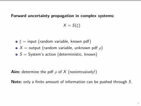
Forward uncertainty propagation in complex systems:
X = S(ξ)
ξ = input (random variable, known pdf)
X = output (random variable, unknown pdf ρ)
S = System’s action (deterministic, known)
Aim: determine the pdf ρ of X (nonintrusively!)
Note: only a finite amount of information can be pushed through S .
2
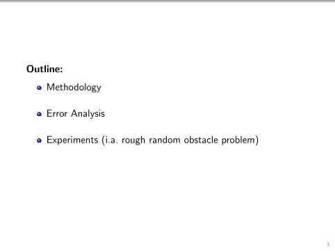
Outline:
Methodology
Error Analysis
Experiments (i.a. rough random obstacle problem)
3
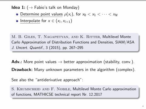
Idea 1: (→ Fabio’s talk on Monday)
Determine point values ρ(xi ), for x0 < x1 < · · · < xN
Interpolate for x ∈ (xi , xi+1)
M. B. Giles, T. Nagapetyan, and K. Ritter, Multilevel Monte
Carlo Approximation of Distribution Functions and Densities, SIAM/ASA
J. Uncert. Quantif., 3 (2015), pp. 267–295
Adv.: More point values → better approximation (stability, conv.).
Drawback: Many unknown parameters in the algorithm (complex).
See also the “antiderivative approach”:
S. Krumscheid and F. Nobile, Multilevel Monte Carlo approximation
of functions, MATHICSE technical report Nr. 12.2017
4
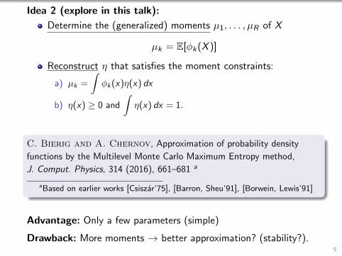
Idea 2 (explore in this talk):
Determine the (generalized) moments µ1, . . . , µR of X
µk = E[φk(X )]
Reconstruct η that satisfies the moment constraints:
a) µk =
∫φk(x)η(x) dx
b) η(x) ≥ 0 and
∫η(x) dx = 1.
C. Bierig and A. Chernov, Approximation of probability density
functions by the Multilevel Monte Carlo Maximum Entropy method,
J. Comput. Physics, 314 (2016), 661–681 a
aBased on earlier works [Csiszar’75], [Barron, Sheu’91], [Borwein, Lewis’91]
Advantage: Only a few parameters (simple)
Drawback: More moments → better approximation? (stability?).5
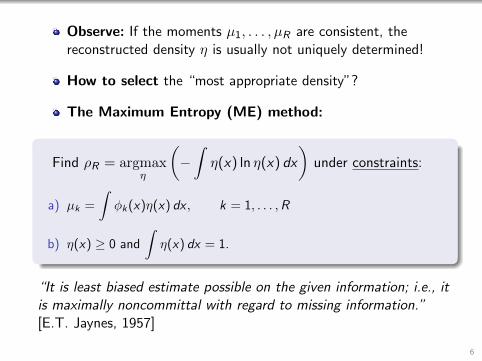
Observe: If the moments µ1, . . . , µR are consistent, thereconstructed density η is usually not uniquely determined!
How to select the “most appropriate density”?
The Maximum Entropy (ME) method:
Find ρR = argmaxη
(−∫η(x) ln η(x) dx
)under constraints:
a) µk =
∫φk(x)η(x) dx , k = 1, . . . ,R
b) η(x) ≥ 0 and
∫η(x) dx = 1.
“It is least biased estimate possible on the given information; i.e., itis maximally noncommittal with regard to missing information.”[E.T. Jaynes, 1957]
6
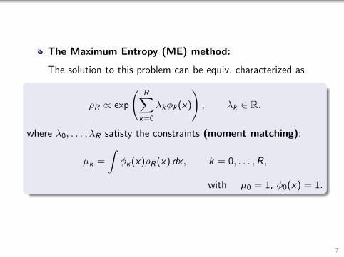
The Maximum Entropy (ME) method:
The solution to this problem can be equiv. characterized as
ρR ∝ exp
(R∑
k=0
λkφk(x)
), λk ∈ R.
where λ0, . . . , λR satisty the constraints (moment matching):
µk =
∫φk(x)ρR(x) dx , k = 0, . . . ,R,
with µ0 = 1, φ0(x) = 1.
7
In this sense:
Entropy maximizationm
moment matching
8
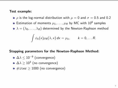
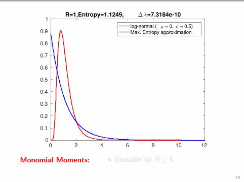
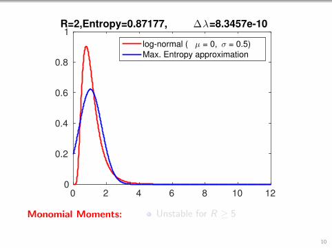
Test example:
ρ is the log-normal distribution with µ = 0 and σ = 0.5 and 0.2
Estimation of moments µ1, . . . , µR by MC with 108 samples
λ = (λ0, . . . , λR) determined by the Newton-Raphson method∫φk(x)ρR(λ, x) dx = µk , k = 0, . . .R.
Stopping parameters for the Newton-Raphson Method:
∆λ ≤ 10−9 (convergence)
∆λ ≥ 103 (no convergence)
#iter ≥ 1000 (no convergence)
9
0 2 4 6 8 10 120
0.1
0.2
0.3
0.4
0.5
0.6
0.7
0.8
0.9
1R=1,Entropy=1.1249, ∆λ=7.3184e-10
log-normal ( µ = 0, σ = 0.5)
Max. Entropy approximation
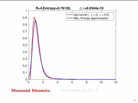
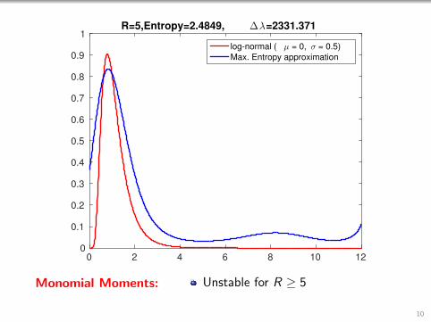
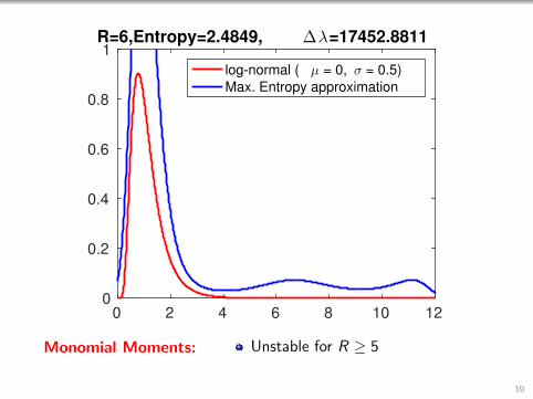
Monomial Moments: Unstable for R ≥ 5
10
0 2 4 6 8 10 120
0.2
0.4
0.6
0.8
1R=2,Entropy=0.87177, ∆λ=8.3457e-10
log-normal ( µ = 0, σ = 0.5)
Max. Entropy approximation
Monomial Moments: Unstable for R ≥ 5
10
0 2 4 6 8 10 120
0.2
0.4
0.6
0.8
1R=3,Entropy=0.84002, ∆λ=8.6141e-10
log-normal ( µ = 0, σ = 0.5)
Max. Entropy approximation
Monomial Moments: Unstable for R ≥ 5
10
0 2 4 6 8 10 120
0.1
0.2
0.3
0.4
0.5
0.6
0.7
0.8
0.9
1R=4,Entropy=0.76128, ∆λ=6.9344e-10
log-normal ( µ = 0, σ = 0.5)
Max. Entropy approximation
Monomial Moments: Unstable for R ≥ 5
10
0 2 4 6 8 10 120
0.1
0.2
0.3
0.4
0.5
0.6
0.7
0.8
0.9
1R=5,Entropy=2.4849, ∆λ=2331.371
log-normal ( µ = 0, σ = 0.5)
Max. Entropy approximation
Monomial Moments: Unstable for R ≥ 5
10
0 2 4 6 8 10 120
0.2
0.4
0.6
0.8
1R=6,Entropy=2.4849, ∆λ=17452.8811
log-normal ( µ = 0, σ = 0.5)
Max. Entropy approximation
Monomial Moments: Unstable for R ≥ 5
10
0 2 4 6 8 10 120
0.1
0.2
0.3
0.4
0.5
0.6
0.7
0.8
0.9
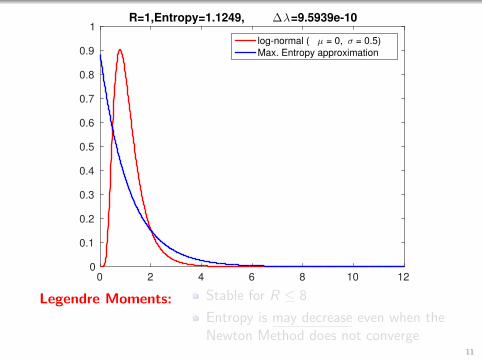
1R=1,Entropy=1.1249, ∆λ=9.5939e-10
log-normal ( µ = 0, σ = 0.5)
Max. Entropy approximation
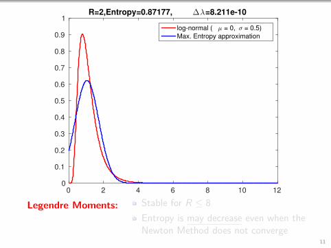
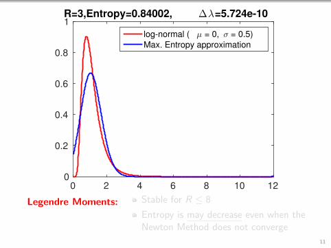
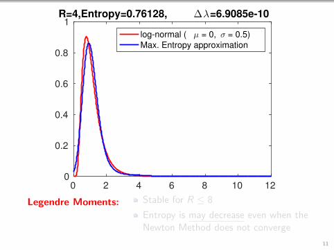
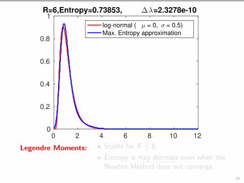
Legendre Moments: Stable for R ≤ 8
Entropy is may decrease even when theNewton Method does not converge
11
0 2 4 6 8 10 120
0.1
0.2
0.3
0.4
0.5
0.6
0.7
0.8
0.9
1R=2,Entropy=0.87177, ∆λ=8.211e-10
log-normal ( µ = 0, σ = 0.5)
Max. Entropy approximation
Legendre Moments: Stable for R ≤ 8
Entropy is may decrease even when theNewton Method does not converge
11
0 2 4 6 8 10 120
0.2
0.4
0.6
0.8
1R=3,Entropy=0.84002, ∆λ=5.724e-10
log-normal ( µ = 0, σ = 0.5)
Max. Entropy approximation
Legendre Moments: Stable for R ≤ 8
Entropy is may decrease even when theNewton Method does not converge
11
0 2 4 6 8 10 120
0.2
0.4
0.6
0.8
1R=4,Entropy=0.76128, ∆λ=6.9085e-10
log-normal ( µ = 0, σ = 0.5)
Max. Entropy approximation
Legendre Moments: Stable for R ≤ 8
Entropy is may decrease even when theNewton Method does not converge
11
0 2 4 6 8 10 120
0.2
0.4
0.6
0.8
1R=6,Entropy=0.73853, ∆λ=2.3278e-10
log-normal ( µ = 0, σ = 0.5)
Max. Entropy approximation
Legendre Moments: Stable for R ≤ 8
Entropy is may decrease even when theNewton Method does not converge
11
0 2 4 6 8 10 120
0.2
0.4
0.6
0.8
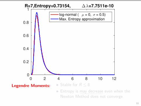
1R=7,Entropy=0.73154, ∆λ=7.7511e-10
log-normal ( µ = 0, σ = 0.5)
Max. Entropy approximation
Legendre Moments: Stable for R ≤ 8
Entropy is may decrease even when theNewton Method does not converge
11
0 2 4 6 8 10 120
0.2
0.4
0.6
0.8
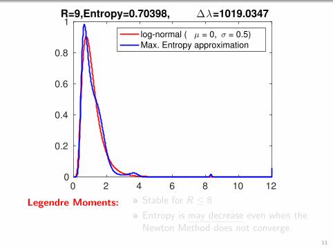
1R=9,Entropy=0.70398, ∆λ=1019.0347
log-normal ( µ = 0, σ = 0.5)
Max. Entropy approximation
Legendre Moments: Stable for R ≤ 8
Entropy is may decrease even when theNewton Method does not converge
11
0 2 4 6 8 10 120
0.2
0.4
0.6
0.8
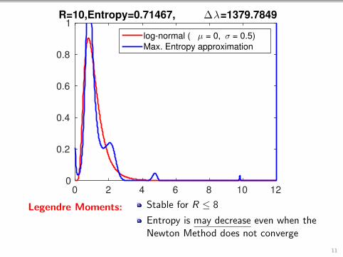
1R=10,Entropy=0.71467, ∆λ=1379.7849
log-normal ( µ = 0, σ = 0.5)
Max. Entropy approximation
Legendre Moments: Stable for R ≤ 8
Entropy is may decrease even when theNewton Method does not converge
11
0 2 4 6 8 10 120
0.2
0.4
0.6
0.8
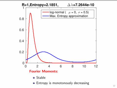
1R=1,Entropy=2.1851, ∆λ=7.2644e-10
log-normal ( µ = 0, σ = 0.5)
Max. Entropy approximation
Fourier Moments:
Stable
Entropy is monotonously decreasing12

0 2 4 6 8 10 120
0.1
0.2
0.3
0.4
0.5
0.6
0.7
0.8
0.9
1R=2,Entropy=0.8924, ∆λ=7.7399e-10
log-normal ( µ = 0, σ = 0.5)
Max. Entropy approximation
Fourier Moments:
Stable
Entropy is monotonously decreasing12
0 2 4 6 8 10 120
0.1
0.2
0.3
0.4
0.5
0.6
0.7
0.8
0.9
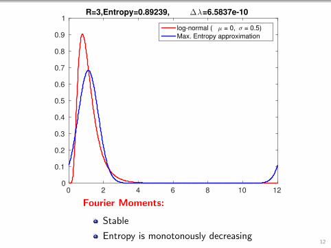
1R=3,Entropy=0.89239, ∆λ=6.5837e-10
log-normal ( µ = 0, σ = 0.5)
Max. Entropy approximation
Fourier Moments:
Stable
Entropy is monotonously decreasing12
0 2 4 6 8 10 120
0.1
0.2
0.3
0.4
0.5
0.6
0.7
0.8
0.9
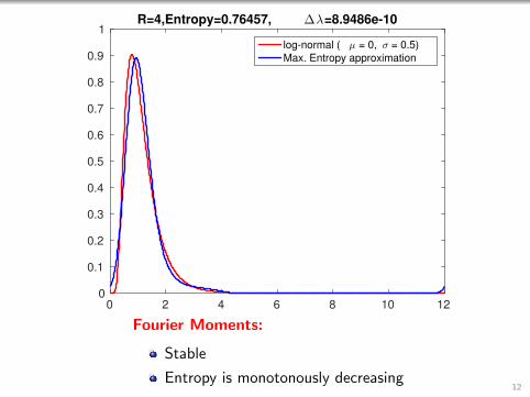
1R=4,Entropy=0.76457, ∆λ=8.9486e-10
log-normal ( µ = 0, σ = 0.5)
Max. Entropy approximation
Fourier Moments:
Stable
Entropy is monotonously decreasing12
0 2 4 6 8 10 120
0.2
0.4
0.6
0.8
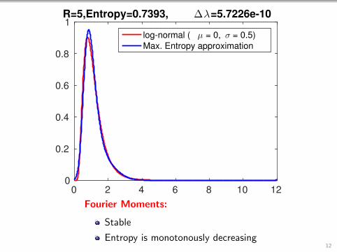
1R=5,Entropy=0.7393, ∆λ=5.7226e-10
log-normal ( µ = 0, σ = 0.5)
Max. Entropy approximation
Fourier Moments:
Stable
Entropy is monotonously decreasing12
0 2 4 6 8 10 120
0.2
0.4
0.6
0.8
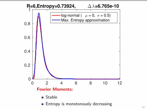
1R=6,Entropy=0.73924, ∆λ=6.765e-10
log-normal ( µ = 0, σ = 0.5)
Max. Entropy approximation
Fourier Moments:
Stable
Entropy is monotonously decreasing12

0 2 4 6 8 10 120
0.2
0.4
0.6
0.8
1R=8,Entropy=0.73161, ∆λ=8.4948e-10
log-normal ( µ = 0, σ = 0.5)
Max. Entropy approximation
Fourier Moments:
Stable
Entropy is monotonously decreasing12

0 2 4 6 8 10 120
0.2
0.4
0.6
0.8
1R=9,Entropy=0.72997, ∆λ=9.0555e-10
log-normal ( µ = 0, σ = 0.5)
Max. Entropy approximation
Fourier Moments:
Stable
Entropy is monotonously decreasing12
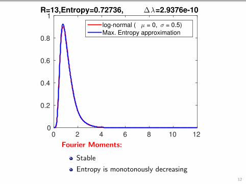
0 2 4 6 8 10 120
0.2
0.4
0.6
0.8
1R=13,Entropy=0.72736, ∆λ=2.9376e-10
log-normal ( µ = 0, σ = 0.5)
Max. Entropy approximation
Fourier Moments:
Stable
Entropy is monotonously decreasing12
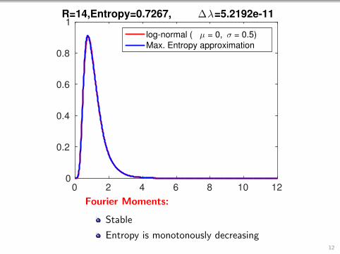
0 2 4 6 8 10 120
0.2
0.4
0.6
0.8
1R=14,Entropy=0.7267, ∆λ=5.2192e-11
log-normal ( µ = 0, σ = 0.5)
Max. Entropy approximation
Fourier Moments:
Stable
Entropy is monotonously decreasing12
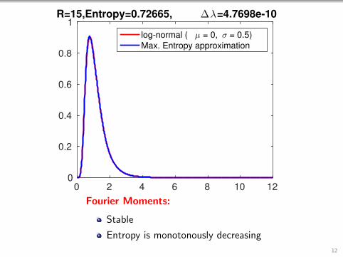
0 2 4 6 8 10 120
0.2
0.4
0.6
0.8
1R=15,Entropy=0.72665, ∆λ=4.7698e-10
log-normal ( µ = 0, σ = 0.5)
Max. Entropy approximation
Fourier Moments:
Stable
Entropy is monotonously decreasing
12

0 2 4 6 8 10 120
0.2
0.4
0.6
0.8
1R=17,Entropy=0.72628, ∆λ=7.7005e-10
log-normal ( µ = 0, σ = 0.5)
Max. Entropy approximation
Fourier Moments:
Stable
Entropy is monotonously decreasing12
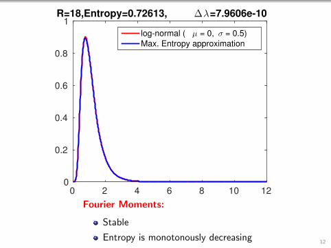
0 2 4 6 8 10 120
0.2
0.4
0.6
0.8
1R=18,Entropy=0.72613, ∆λ=7.9606e-10
log-normal ( µ = 0, σ = 0.5)
Max. Entropy approximation
Fourier Moments:
Stable
Entropy is monotonously decreasing12
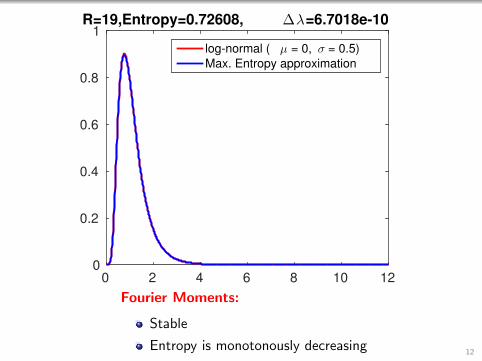
0 2 4 6 8 10 120
0.2
0.4
0.6
0.8
1R=19,Entropy=0.72608, ∆λ=6.7018e-10
log-normal ( µ = 0, σ = 0.5)
Max. Entropy approximation
Fourier Moments:
Stable
Entropy is monotonously decreasing12
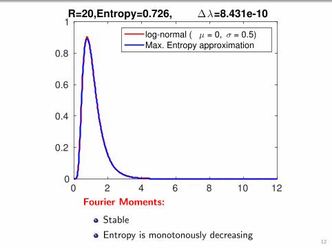
0 2 4 6 8 10 120
0.2
0.4
0.6
0.8
1R=20,Entropy=0.726, ∆λ=8.431e-10
log-normal ( µ = 0, σ = 0.5)
Max. Entropy approximation
Fourier Moments:
Stable
Entropy is monotonously decreasing12
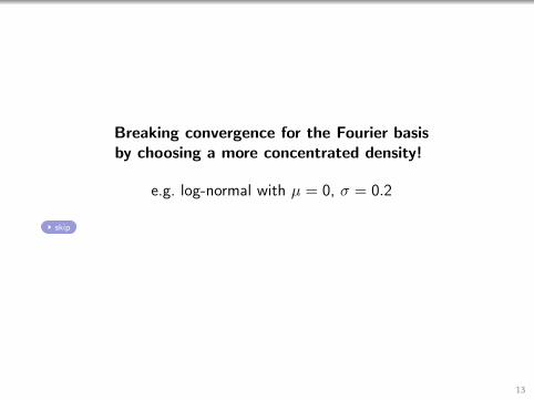
Breaking convergence for the Fourier basisby choosing a more concentrated density!
e.g. log-normal with µ = 0, σ = 0.2
skip
13
0 2 4 6 8 10 120
0.5
1
1.5
2
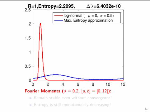
2.5R=1,Entropy=2.2095, ∆λ=6.4032e-10
log-normal ( µ = 0, σ = 0.5)
Max. Entropy approximation
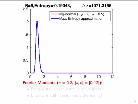
Fourier Moments (σ = 0.2, [a, b] = [0, 12]):
Remain stable even without convergence!
Entropy is still monotonously decreasing!14
0 2 4 6 8 10 120
0.5
1
1.5
2
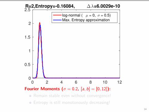
2.5R=2,Entropy=-0.16084, ∆λ=6.0029e-10
log-normal ( µ = 0, σ = 0.5)
Max. Entropy approximation
Fourier Moments (σ = 0.2, [a, b] = [0, 12]):
Remain stable even without convergence!
Entropy is still monotonously decreasing!
14
0 2 4 6 8 10 120
0.5
1
1.5
2
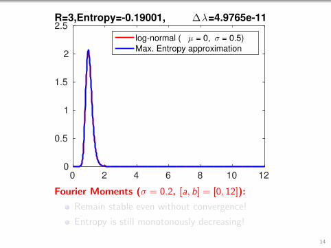
2.5R=3,Entropy=-0.19001, ∆λ=4.9765e-11
log-normal ( µ = 0, σ = 0.5)
Max. Entropy approximation
Fourier Moments (σ = 0.2, [a, b] = [0, 12]):
Remain stable even without convergence!
Entropy is still monotonously decreasing!
14
0 2 4 6 8 10 120
0.5
1
1.5
2
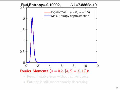
2.5R=4,Entropy=-0.19002, ∆λ=7.8862e-10
log-normal ( µ = 0, σ = 0.5)
Max. Entropy approximation
Fourier Moments (σ = 0.2, [a, b] = [0, 12]):
Remain stable even without convergence!
Entropy is still monotonously decreasing!
14
0 2 4 6 8 10 120
0.5
1
1.5
2
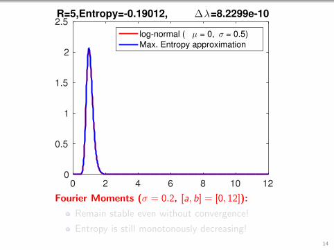
2.5R=5,Entropy=-0.19012, ∆λ=8.2299e-10
log-normal ( µ = 0, σ = 0.5)
Max. Entropy approximation
Fourier Moments (σ = 0.2, [a, b] = [0, 12]):
Remain stable even without convergence!
Entropy is still monotonously decreasing!
14
0 2 4 6 8 10 120
0.5
1
1.5
2
2.5R=6,Entropy=-0.19048, ∆λ=1071.3155
log-normal ( µ = 0, σ = 0.5)
Max. Entropy approximation
Fourier Moments (σ = 0.2, [a, b] = [0, 12]):
Remain stable even without convergence!
Entropy is still monotonously decreasing!
14
0 2 4 6 8 10 120
0.5
1
1.5
2
2.5R=8,Entropy=-0.19054, ∆λ=1011.0382
log-normal ( µ = 0, σ = 0.5)
Max. Entropy approximation
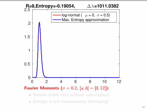
Fourier Moments (σ = 0.2, [a, b] = [0, 12]):
Remain stable even without convergence!
Entropy is still monotonously decreasing!14
0 2 4 6 8 10 120
0.5
1
1.5
2
2.5R=9,Entropy=-0.1905, ∆λ=2342.9086
log-normal ( µ = 0, σ = 0.5)
Max. Entropy approximation
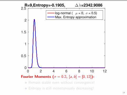
Fourier Moments (σ = 0.2, [a, b] = [0, 12]):
Remain stable even without convergence!
Entropy is still monotonously decreasing!14
0 2 4 6 8 10 120
0.5
1
1.5
2
2.5R=13,Entropy=-0.19055, ∆λ=1117.2321
log-normal ( µ = 0, σ = 0.5)
Max. Entropy approximation
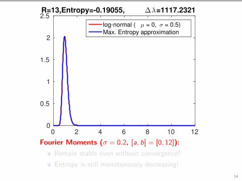
Fourier Moments (σ = 0.2, [a, b] = [0, 12]):
Remain stable even without convergence!
Entropy is still monotonously decreasing!
14
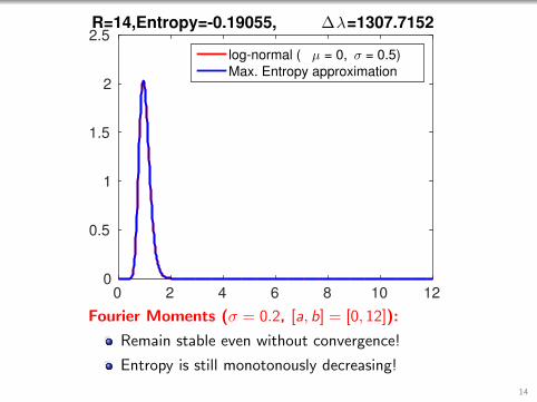
0 2 4 6 8 10 120
0.5
1
1.5
2
2.5R=14,Entropy=-0.19055, ∆λ=1307.7152
log-normal ( µ = 0, σ = 0.5)
Max. Entropy approximation
Fourier Moments (σ = 0.2, [a, b] = [0, 12]):
Remain stable even without convergence!
Entropy is still monotonously decreasing!
14

0 2 4 6 8 10 120
0.5
1
1.5
2
2.5R=15,Entropy=-0.19055, ∆λ=7575.1711
log-normal ( µ = 0, σ = 0.5)
Max. Entropy approximation
Fourier Moments (σ = 0.2, [a, b] = [0, 12]):
Remain stable even without convergence!
Entropy is still monotonously decreasing!
14

0 2 4 6 8 10 120
0.5
1
1.5
2
2.5R=16,Entropy=-0.19055, ∆λ=1283.0868
log-normal ( µ = 0, σ = 0.5)
Max. Entropy approximation
Fourier Moments (σ = 0.2, [a, b] = [0, 12]):
Remain stable even without convergence!
Entropy is still monotonously decreasing!
14
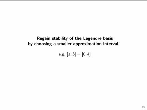
Regain stability of the Legendre basisby choosing a smaller approximation interval!
e.g. [a, b] = [0, 4]
15
0 1 2 3 40
0.5
1
1.5
2
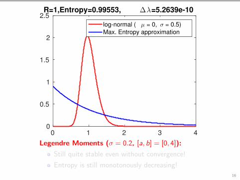
2.5R=1,Entropy=0.99553, ∆λ=5.2639e-10
log-normal ( µ = 0, σ = 0.5)
Max. Entropy approximation
Legendre Moments (σ = 0.2, [a, b] = [0, 4]):
Still quite stable even without convergence!
Entropy is still monotonously decreasing!
16
0 1 2 3 40
0.5
1
1.5
2
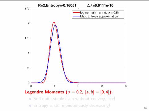
2.5R=2,Entropy=-0.16051, ∆λ=6.6111e-10
log-normal ( µ = 0, σ = 0.5)
Max. Entropy approximation
Legendre Moments (σ = 0.2, [a, b] = [0, 4]):
Still quite stable even without convergence!
Entropy is still monotonously decreasing!16
0 1 2 3 40
0.5
1
1.5
2
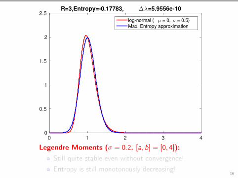
2.5R=3,Entropy=-0.17783, ∆λ=5.9556e-10
log-normal ( µ = 0, σ = 0.5)
Max. Entropy approximation
Legendre Moments (σ = 0.2, [a, b] = [0, 4]):
Still quite stable even without convergence!
Entropy is still monotonously decreasing!16
0 1 2 3 40
0.5
1
1.5
2
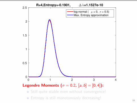
2.5R=4,Entropy=-0.1901, ∆λ=1.1527e-10
log-normal ( µ = 0, σ = 0.5)
Max. Entropy approximation
Legendre Moments (σ = 0.2, [a, b] = [0, 4]):
Still quite stable even without convergence!
Entropy is still monotonously decreasing!16
0 1 2 3 40
0.5
1
1.5
2
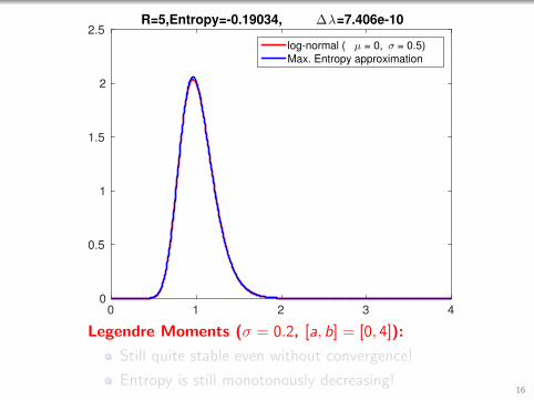
2.5R=5,Entropy=-0.19034, ∆λ=7.406e-10
log-normal ( µ = 0, σ = 0.5)
Max. Entropy approximation
Legendre Moments (σ = 0.2, [a, b] = [0, 4]):
Still quite stable even without convergence!
Entropy is still monotonously decreasing!16

0 1 2 3 40
0.5
1
1.5
2
2.5R=6,Entropy=-0.19054, ∆λ=8.5076e-10
log-normal ( µ = 0, σ = 0.5)
Max. Entropy approximation
Legendre Moments (σ = 0.2, [a, b] = [0, 4]):
Still quite stable even without convergence!
Entropy is still monotonously decreasing!16

0 1 2 3 40
0.5
1
1.5
2
2.5R=8,Entropy=-0.19055, ∆λ=2.0455e-06
log-normal ( µ = 0, σ = 0.5)
Max. Entropy approximation
Legendre Moments (σ = 0.2, [a, b] = [0, 4]):
Still quite stable even without convergence!
Entropy is still monotonously decreasing!16

0 1 2 3 40
0.5
1
1.5
2
2.5R=9,Entropy=-0.19055, ∆λ=3.6249e-07
log-normal ( µ = 0, σ = 0.5)
Max. Entropy approximation
Legendre Moments (σ = 0.2, [a, b] = [0, 4]):
Still quite stable even without convergence!
Entropy is still monotonously decreasing!16

0 1 2 3 40
0.5
1
1.5
2
2.5R=13,Entropy=-0.19055, ∆λ=2.6296e-05
log-normal ( µ = 0, σ = 0.5)
Max. Entropy approximation
Legendre Moments (σ = 0.2, [a, b] = [0, 4]):
Still quite stable even without convergence!
Entropy is still monotonously decreasing!16

0 1 2 3 40
0.5
1
1.5
2
2.5R=14,Entropy=-0.19055, ∆λ=4.1482e-05
log-normal ( µ = 0, σ = 0.5)
Max. Entropy approximation
Legendre Moments (σ = 0.2, [a, b] = [0, 4]):
Still quite stable even without convergence!
Entropy is still monotonously decreasing!16

0 1 2 3 40
0.5
1
1.5
2
2.5R=15,Entropy=-0.19055, ∆λ=1272.7572
log-normal ( µ = 0, σ = 0.5)
Max. Entropy approximation
Legendre Moments (σ = 0.2, [a, b] = [0, 4]):
Still quite stable even without convergence!
Entropy is still monotonously decreasing!16
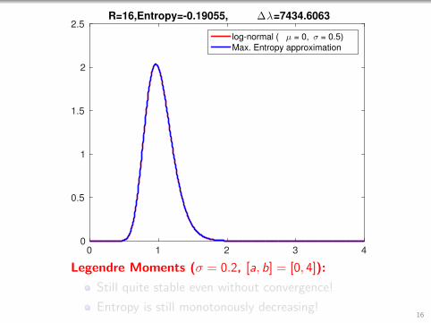
0 1 2 3 40
0.5
1
1.5
2
2.5R=16,Entropy=-0.19055, ∆λ=7434.6063
log-normal ( µ = 0, σ = 0.5)
Max. Entropy approximation
Legendre Moments (σ = 0.2, [a, b] = [0, 4]):
Still quite stable even without convergence!
Entropy is still monotonously decreasing!16

0 1 2 3 40
0.5
1
1.5
2
2.5R=17,Entropy=-0.19055, ∆λ=2095.7446
log-normal ( µ = 0, σ = 0.5)
Max. Entropy approximation
Legendre Moments (σ = 0.2, [a, b] = [0, 4]):
Still quite stable even without convergence!
Entropy is still monotonously decreasing!16
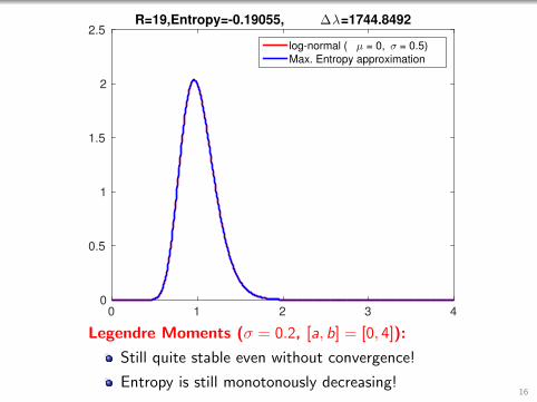
0 1 2 3 40
0.5
1
1.5
2
2.5R=19,Entropy=-0.19055, ∆λ=1744.8492
log-normal ( µ = 0, σ = 0.5)
Max. Entropy approximation
Legendre Moments (σ = 0.2, [a, b] = [0, 4]):
Still quite stable even without convergence!
Entropy is still monotonously decreasing!16

0 1 2 3 40
0.5
1
1.5
2
2.5R=20,Entropy=-0.19055, ∆λ=2019.5142
log-normal ( µ = 0, σ = 0.5)
Max. Entropy approximation
Legendre Moments (σ = 0.2, [a, b] = [0, 4]):
Still quite stable even without convergence!
Entropy is still monotonously decreasing!16
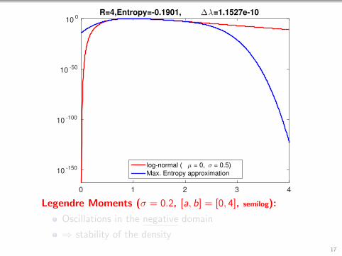
0 1 2 3 4
10-150
10-100
10-50
100
R=1,Entropy=0.99553, ∆λ=5.2639e-10
log-normal ( µ = 0, σ = 0.5)
Max. Entropy approximation
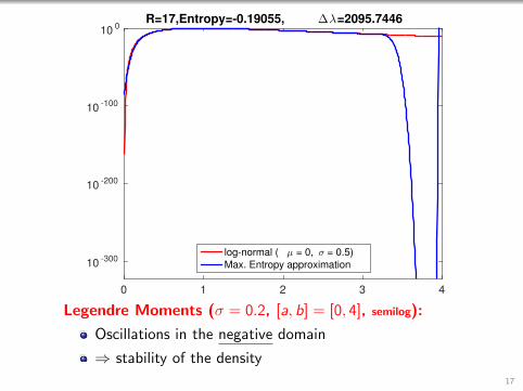
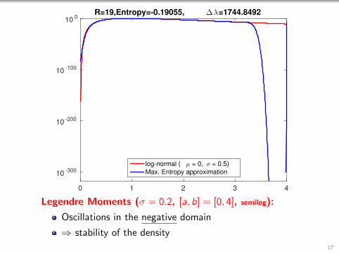
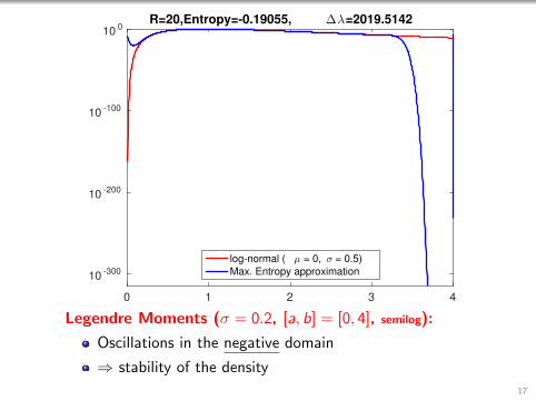
Legendre Moments (σ = 0.2, [a, b] = [0, 4], semilog):
Oscillations in the negative domain
⇒ stability of the density
17
0 1 2 3 4
10-150
10-100
10-50
100
R=2,Entropy=-0.16051, ∆λ=6.6111e-10
log-normal ( µ = 0, σ = 0.5)
Max. Entropy approximation
Legendre Moments (σ = 0.2, [a, b] = [0, 4], semilog):
Oscillations in the negative domain
⇒ stability of the density
17
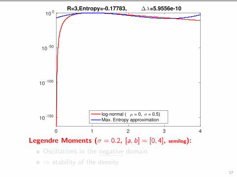
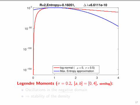
0 1 2 3 4
10-150
10-100
10-50
100
R=3,Entropy=-0.17783, ∆λ=5.9556e-10
log-normal ( µ = 0, σ = 0.5)
Max. Entropy approximation
Legendre Moments (σ = 0.2, [a, b] = [0, 4], semilog):
Oscillations in the negative domain
⇒ stability of the density
17
0 1 2 3 4
10-150
10-100
10-50
100
R=4,Entropy=-0.1901, ∆λ=1.1527e-10
log-normal ( µ = 0, σ = 0.5)
Max. Entropy approximation
Legendre Moments (σ = 0.2, [a, b] = [0, 4], semilog):
Oscillations in the negative domain
⇒ stability of the density
17

0 1 2 3 4
10-150
10-100
10-50
100
R=5,Entropy=-0.19034, ∆λ=7.406e-10
log-normal ( µ = 0, σ = 0.5)
Max. Entropy approximation
Legendre Moments (σ = 0.2, [a, b] = [0, 4], semilog):
Oscillations in the negative domain
⇒ stability of the density
17
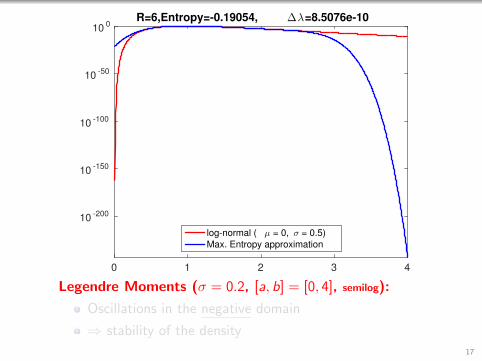
0 1 2 3 4
10-200
10-150
10-100
10-50
100
R=6,Entropy=-0.19054, ∆λ=8.5076e-10
log-normal ( µ = 0, σ = 0.5)
Max. Entropy approximation
Legendre Moments (σ = 0.2, [a, b] = [0, 4], semilog):
Oscillations in the negative domain
⇒ stability of the density
17
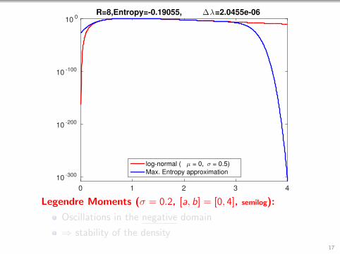
0 1 2 3 4
10-300
10-200
10-100
100
R=8,Entropy=-0.19055, ∆λ=2.0455e-06
log-normal ( µ = 0, σ = 0.5)
Max. Entropy approximation
Legendre Moments (σ = 0.2, [a, b] = [0, 4], semilog):
Oscillations in the negative domain
⇒ stability of the density
17
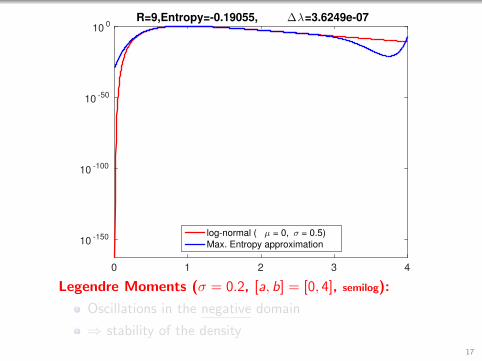
0 1 2 3 4
10-150
10-100
10-50
100
R=9,Entropy=-0.19055, ∆λ=3.6249e-07
log-normal ( µ = 0, σ = 0.5)
Max. Entropy approximation
Legendre Moments (σ = 0.2, [a, b] = [0, 4], semilog):
Oscillations in the negative domain
⇒ stability of the density
17
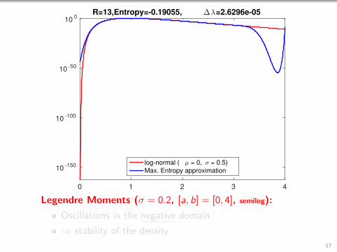
0 1 2 3 4
10-150
10-100
10-50
100
R=13,Entropy=-0.19055, ∆λ=2.6296e-05
log-normal ( µ = 0, σ = 0.5)
Max. Entropy approximation
Legendre Moments (σ = 0.2, [a, b] = [0, 4], semilog):
Oscillations in the negative domain
⇒ stability of the density
17
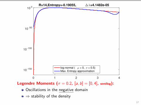
0 1 2 3 4
10-150
10-100
10-50
100
R=14,Entropy=-0.19055, ∆λ=4.1482e-05
log-normal ( µ = 0, σ = 0.5)
Max. Entropy approximation
Legendre Moments (σ = 0.2, [a, b] = [0, 4], semilog):
Oscillations in the negative domain
⇒ stability of the density
17
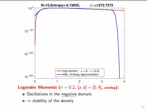
0 1 2 3 4
10-300
10-200
10-100
100
R=15,Entropy=-0.19055, ∆λ=1272.7572
log-normal ( µ = 0, σ = 0.5)
Max. Entropy approximation
Legendre Moments (σ = 0.2, [a, b] = [0, 4], semilog):
Oscillations in the negative domain
⇒ stability of the density
17
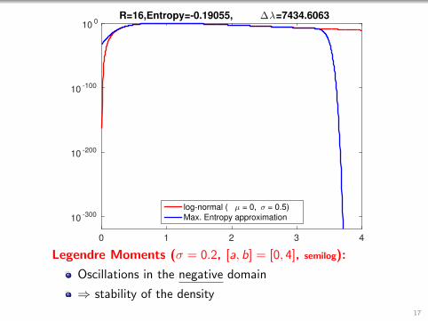
0 1 2 3 4
10-300
10-200
10-100
100
R=16,Entropy=-0.19055, ∆λ=7434.6063
log-normal ( µ = 0, σ = 0.5)
Max. Entropy approximation
Legendre Moments (σ = 0.2, [a, b] = [0, 4], semilog):
Oscillations in the negative domain
⇒ stability of the density
17
0 1 2 3 4
10-300
10-200
10-100
100
R=17,Entropy=-0.19055, ∆λ=2095.7446
log-normal ( µ = 0, σ = 0.5)
Max. Entropy approximation
Legendre Moments (σ = 0.2, [a, b] = [0, 4], semilog):
Oscillations in the negative domain
⇒ stability of the density
17
0 1 2 3 4
10-300
10-200
10-100
100
R=19,Entropy=-0.19055, ∆λ=1744.8492
log-normal ( µ = 0, σ = 0.5)
Max. Entropy approximation
Legendre Moments (σ = 0.2, [a, b] = [0, 4], semilog):
Oscillations in the negative domain
⇒ stability of the density
17
0 1 2 3 4
10-300
10-200
10-100
100
R=20,Entropy=-0.19055, ∆λ=2019.5142
log-normal ( µ = 0, σ = 0.5)
Max. Entropy approximation
Legendre Moments (σ = 0.2, [a, b] = [0, 4], semilog):
Oscillations in the negative domain
⇒ stability of the density
17
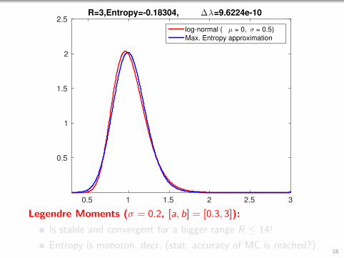
0.5 1 1.5 2 2.5 3
0.5
1
1.5
2
2.5R=2,Entropy=-0.16075, ∆λ=5.1766e-10
log-normal ( µ = 0, σ = 0.5)
Max. Entropy approximation
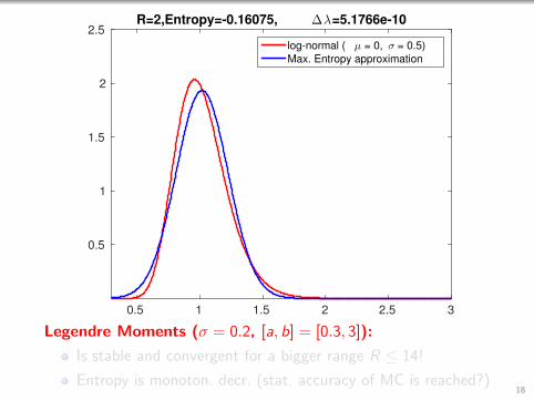
Legendre Moments (σ = 0.2, [a, b] = [0.3, 3]):
Is stable and convergent for a bigger range R ≤ 14!
Entropy is monoton. decr. (stat. accuracy of MC is reached?)18
0.5 1 1.5 2 2.5 3
0.5
1
1.5
2
2.5R=3,Entropy=-0.18304, ∆λ=9.6224e-10
log-normal ( µ = 0, σ = 0.5)
Max. Entropy approximation
Legendre Moments (σ = 0.2, [a, b] = [0.3, 3]):
Is stable and convergent for a bigger range R ≤ 14!
Entropy is monoton. decr. (stat. accuracy of MC is reached?)18
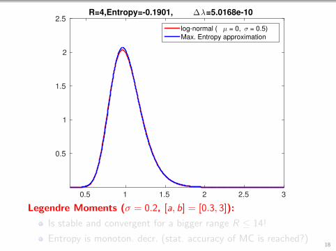
0.5 1 1.5 2 2.5 3
0.5
1
1.5
2
2.5R=4,Entropy=-0.1901, ∆λ=5.0168e-10
log-normal ( µ = 0, σ = 0.5)
Max. Entropy approximation
Legendre Moments (σ = 0.2, [a, b] = [0.3, 3]):
Is stable and convergent for a bigger range R ≤ 14!
Entropy is monoton. decr. (stat. accuracy of MC is reached?)18

0.5 1 1.5 2 2.5 3
0.5
1
1.5
2
2.5R=5,Entropy=-0.19043, ∆λ=5.9985e-10
log-normal ( µ = 0, σ = 0.5)
Max. Entropy approximation
Legendre Moments (σ = 0.2, [a, b] = [0.3, 3]):
Is stable and convergent for a bigger range R ≤ 14!
Entropy is monoton. decr. (stat. accuracy of MC is reached?)18
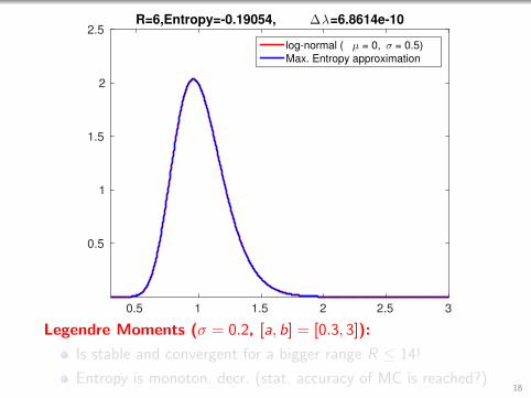
0.5 1 1.5 2 2.5 3
0.5
1
1.5
2
2.5R=6,Entropy=-0.19054, ∆λ=6.8614e-10
log-normal ( µ = 0, σ = 0.5)
Max. Entropy approximation
Legendre Moments (σ = 0.2, [a, b] = [0.3, 3]):
Is stable and convergent for a bigger range R ≤ 14!
Entropy is monoton. decr. (stat. accuracy of MC is reached?)18
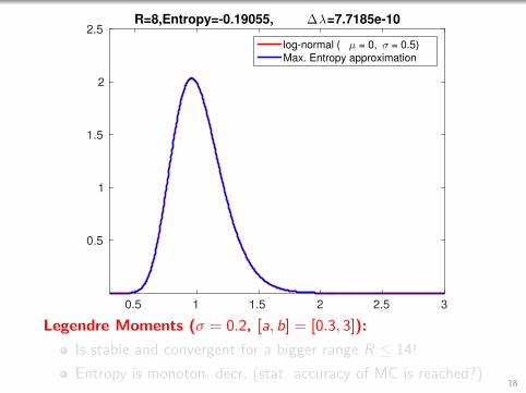
0.5 1 1.5 2 2.5 3
0.5
1
1.5
2
2.5R=8,Entropy=-0.19055, ∆λ=7.7185e-10
log-normal ( µ = 0, σ = 0.5)
Max. Entropy approximation
Legendre Moments (σ = 0.2, [a, b] = [0.3, 3]):
Is stable and convergent for a bigger range R ≤ 14!
Entropy is monoton. decr. (stat. accuracy of MC is reached?)18

0.5 1 1.5 2 2.5 3
0.5
1
1.5
2
2.5R=9,Entropy=-0.19055, ∆λ=6.5113e-10
log-normal ( µ = 0, σ = 0.5)
Max. Entropy approximation
Legendre Moments (σ = 0.2, [a, b] = [0.3, 3]):
Is stable and convergent for a bigger range R ≤ 14!
Entropy is monoton. decr. (stat. accuracy of MC is reached?)18

0.5 1 1.5 2 2.5 3
0.5
1
1.5
2
2.5R=13,Entropy=-0.19055, ∆λ=8.1749e-10
log-normal ( µ = 0, σ = 0.5)
Max. Entropy approximation
Legendre Moments (σ = 0.2, [a, b] = [0.3, 3]):
Is stable and convergent for a bigger range R ≤ 14!
Entropy is monoton. decr. (stat. accuracy of MC is reached?)18
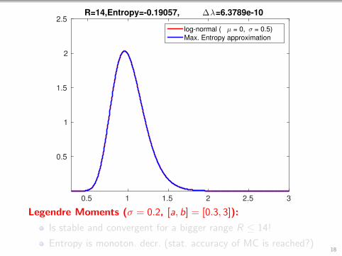
0.5 1 1.5 2 2.5 3
0.5
1
1.5
2
2.5R=14,Entropy=-0.19057, ∆λ=6.3789e-10
log-normal ( µ = 0, σ = 0.5)
Max. Entropy approximation
Legendre Moments (σ = 0.2, [a, b] = [0.3, 3]):
Is stable and convergent for a bigger range R ≤ 14!
Entropy is monoton. decr. (stat. accuracy of MC is reached?)18
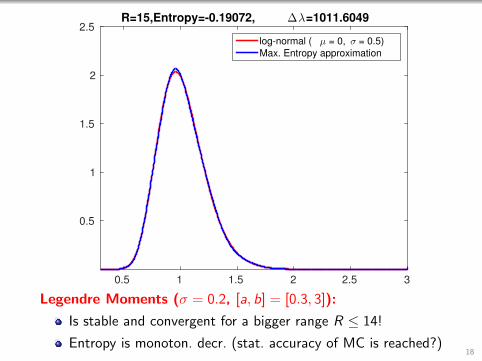
0.5 1 1.5 2 2.5 3
0.5
1
1.5
2
2.5R=15,Entropy=-0.19072, ∆λ=1011.6049
log-normal ( µ = 0, σ = 0.5)
Max. Entropy approximation
Legendre Moments (σ = 0.2, [a, b] = [0.3, 3]):
Is stable and convergent for a bigger range R ≤ 14!
Entropy is monoton. decr. (stat. accuracy of MC is reached?)18
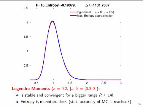
0.5 1 1.5 2 2.5 3
0.5
1
1.5
2
2.5R=16,Entropy=-0.19079, ∆λ=1131.7607
log-normal ( µ = 0, σ = 0.5)
Max. Entropy approximation
Legendre Moments (σ = 0.2, [a, b] = [0.3, 3]):
Is stable and convergent for a bigger range R ≤ 14!
Entropy is monoton. decr. (stat. accuracy of MC is reached?)18
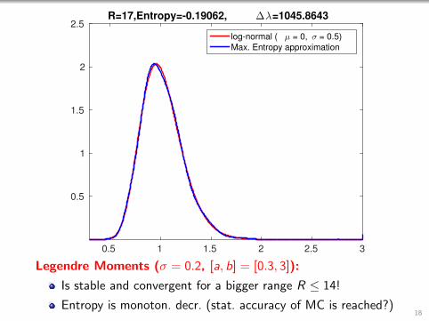
0.5 1 1.5 2 2.5 3
0.5
1
1.5
2
2.5R=17,Entropy=-0.19062, ∆λ=1045.8643
log-normal ( µ = 0, σ = 0.5)
Max. Entropy approximation
Legendre Moments (σ = 0.2, [a, b] = [0.3, 3]):
Is stable and convergent for a bigger range R ≤ 14!
Entropy is monoton. decr. (stat. accuracy of MC is reached?)18
0.5 1 1.5 2 2.5 3
0.5
1
1.5
2
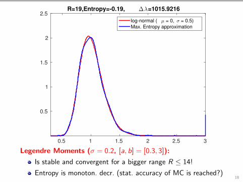
2.5R=19,Entropy=-0.19, ∆λ=1015.9216
log-normal ( µ = 0, σ = 0.5)
Max. Entropy approximation
Legendre Moments (σ = 0.2, [a, b] = [0.3, 3]):
Is stable and convergent for a bigger range R ≤ 14!
Entropy is monoton. decr. (stat. accuracy of MC is reached?)18
0.5 1 1.5 2 2.5 3
0.5
1
1.5
2
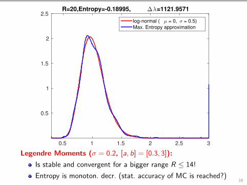
2.5R=20,Entropy=-0.18995, ∆λ=1121.9571
log-normal ( µ = 0, σ = 0.5)
Max. Entropy approximation
Legendre Moments (σ = 0.2, [a, b] = [0.3, 3]):
Is stable and convergent for a bigger range R ≤ 14!
Entropy is monoton. decr. (stat. accuracy of MC is reached?)18
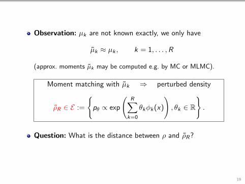
Observation: µk are not known exactly, we only have
µk ≈ µk , k = 1, . . . ,R
(approx. moments µk may be computed e.g. by MC or MLMC).
Moment matching with µk ⇒ perturbed density
ρR ∈ E :=
{pθ ∝ exp
(R∑
k=0
θkφk(x)
), θk ∈ R
}.
Question: What is the distance between ρ and ρR?
19
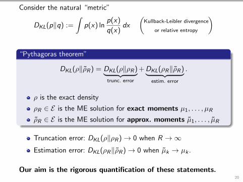
Consider the natural “metric”
DKL(p‖q) :=
∫p(x) ln
p(x)
q(x)dx
(Kullback-Leibler divergence
or relative entropy
)
“Pythagoras theorem”
DKL(ρ‖ρR) = DKL(ρ‖ρR)︸ ︷︷ ︸trunc. error
+DKL(ρR‖ρR)︸ ︷︷ ︸estim. error
.
ρ is the exact density
ρR ∈ E is the ME solution for exact moments µ1, . . . , µR
ρR ∈ E is the ME solution for approx. moments µ1, . . . , µR
Truncation error: DKL(ρ‖ρR)→ 0 when R →∞Estimation error: DKL(ρR‖ρR)→ 0 when µk → µk .
Our aim is the rigorous quantification of these statements.20
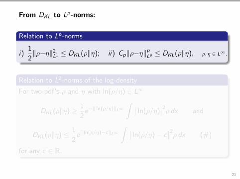
From DKL to Lp-norms:
Relation to Lp-norms
i)1
2‖ρ−η‖2L1 ≤ DKL(ρ‖η); ii) Cp‖ρ−η‖pLp ≤ DKL(ρ‖η), ρ, η ∈ L∞.
Relation to L2-norms of the log-density
For two pdf’s ρ and η with ln(ρ/η) ∈ L∞
DKL(ρ‖η) ≥ 1
2e−‖ ln(ρ/η)‖L∞
∫ ∣∣ ln(ρ/η)∣∣2ρ dx and
DKL(ρ‖η) ≤ 1
2e‖ ln(ρ/η)−c‖L∞
∫ ∣∣ ln(ρ/η)− c∣∣2ρ dx (#)
for any c ∈ R.
21
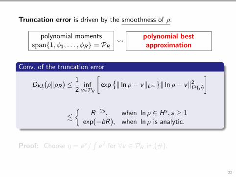
Truncation error is driven by the smoothness of ρ:
polynomial momentsspan{1, φ1, . . . , φR} = PR
polynomial bestapproximation
Conv. of the truncation error
DKL(ρ‖ρR) ≤ 1
2inf
v∈PR
[exp
{‖ ln ρ− v‖L∞
}‖ ln ρ− v‖2L2(ρ)
]
.
{R−2s , when ln ρ ∈ Hs , s ≥ 1
exp(−bR), when ln ρ is analytic.
Proof: Choose η = ev/∫ev for ∀v ∈ PR in (#).
22
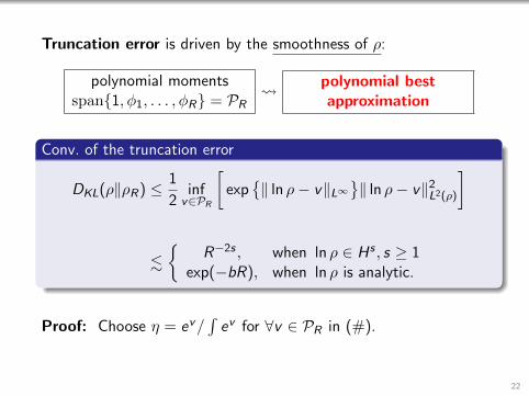
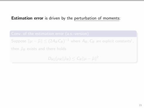
Estimation error is driven by the perturbation of moments:
Conv. of the estimation error (a.s.-version)
Suppose ‖µ− µ‖ ≤ (2ARCR)−1 where AR ,CR are explicit constants†,
then ρR exists and there holds
DKL(ρR‖ρR) ≤ CR‖µ− µ‖2
23
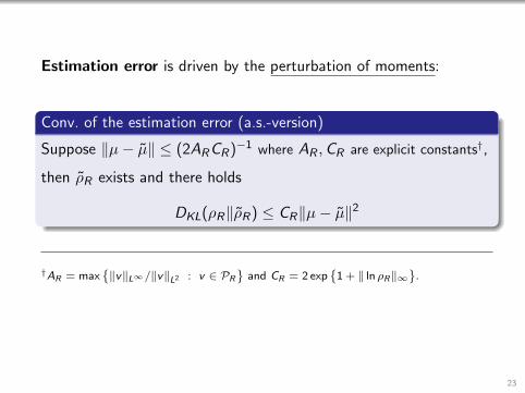
Estimation error is driven by the perturbation of moments:
Conv. of the estimation error (a.s.-version)
Suppose ‖µ− µ‖ ≤ (2ARCR)−1 where AR ,CR are explicit constants†,
then ρR exists and there holds
DKL(ρR‖ρR) ≤ CR‖µ− µ‖2
†AR = max{‖v‖L∞/‖v‖L2 : v ∈ PR
}and CR = 2 exp
{1 + ‖ ln ρR‖∞
}.
23
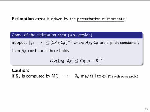
Estimation error is driven by the perturbation of moments:
Conv. of the estimation error (a.s.-version)
Suppose ‖µ− µ‖ ≤ (2ARCR)−1 where AR ,CR are explicit constants†,
then ρR exists and there holds
DKL(ρR‖ρR) ≤ CR‖µ− µ‖2
Caution:If µk is computed by MC ⇒ ρR may fail to exist (with some prob.)
23
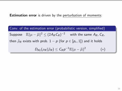
Estimation error is driven by the perturbation of moments:
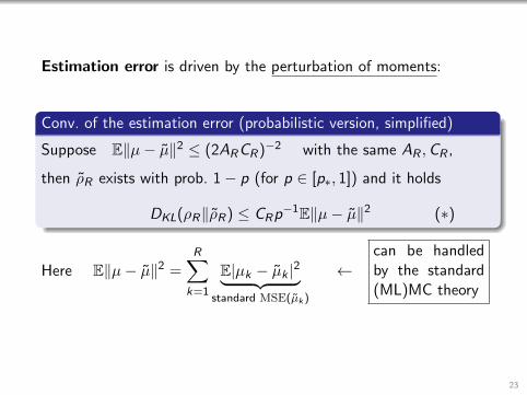
Conv. of the estimation error (probabilistic version, simplified)
Suppose E‖µ− µ‖2 ≤ (2ARCR)−2 with the same AR ,CR ,
then ρR exists with prob. 1− p (for p ∈ [p∗, 1]) and it holds
DKL(ρR‖ρR) ≤ CRp−1E‖µ− µ‖2 (∗)
23
Estimation error is driven by the perturbation of moments:
Conv. of the estimation error (probabilistic version, simplified)
Suppose E‖µ− µ‖2 ≤ (2ARCR)−2 with the same AR ,CR ,
then ρR exists with prob. 1− p (for p ∈ [p∗, 1]) and it holds
DKL(ρR‖ρR) ≤ CRp−1E‖µ− µ‖2 (∗)
Here E‖µ− µ‖2 =R∑
k=1
E|µk − µk |2︸ ︷︷ ︸standard MSE(µk )
←can be handledby the standard(ML)MC theory
23
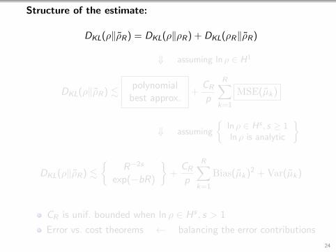
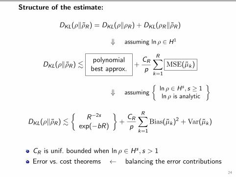
Structure of the estimate:
DKL(ρ‖ρR) = DKL(ρ‖ρR) + DKL(ρR‖ρR)
⇓ assuming ln ρ ∈ H1
DKL(ρ‖ρR) .polynomial
best approx.+
CR
p
R∑k=1
MSE(µk)
⇓ assuming
{ln ρ ∈ Hs , s ≥ 1ln ρ is analytic
}
DKL(ρ‖ρR) .
{R−2s
exp(−bR)
}+
CR
p
R∑k=1
Bias(µk)2 + Var(µk)
CR is unif. bounded when ln ρ ∈ Hs , s > 1
Error vs. cost theorems ← balancing the error contributions
24
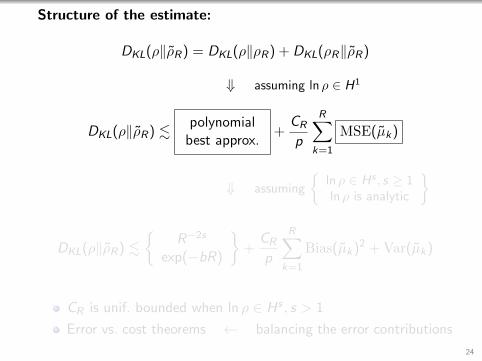
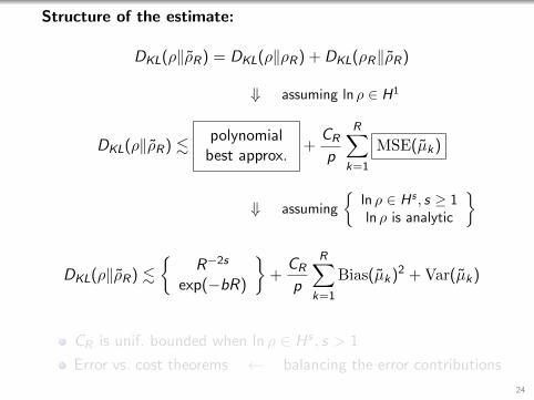
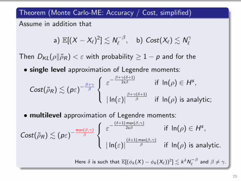
Theorem (Monte Carlo-ME: Accuracy / Cost, simplified)
Assume in addition that
a) E[(X − X`)2] . N−β` , b) Cost(X`) . Nγ
`
Then DKL(ρ‖ρR) < ε with probability ≥ 1− p and for the
• single level approximation of Legendre moments:
Cost(ρR) . (pε)−β+γβ
ε−β+γ(δ+1)
2sβ if ln(ρ) ∈ Hs ,
| ln(ε)|β+γ(δ+1)
β if ln(ρ) is analytic;
• multilevel approximation of Legendre moments:
Cost(ρR) . (pε)−max(β,γ)
β
ε− (δ+1) max(β,γ)
2sβ if ln(ρ) ∈ Hs ,
| ln(ε)|(δ+1) max(β,γ)
β if ln(ρ) is analytic.
Here δ is such that E[(φk (X )− φk (X`))2] . kδN−β` and β 6= γ.
25
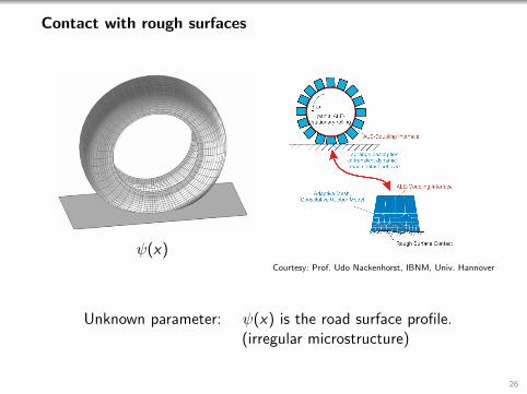
Contact with rough surfaces
ψ(x)Courtesy: Prof. Udo Nackenhorst, IBNM, Univ. Hannover
Unknown parameter: ψ(x) is the road surface profile.(irregular microstructure)
26
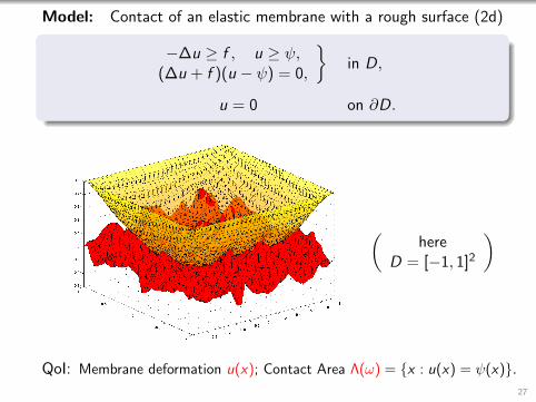
Model: Contact of an elastic membrane with a rough surface (2d)
−∆u ≥ f , u ≥ ψ,(∆u + f )(u − ψ) = 0,
}in D,
u = 0 on ∂D.
(here
D = [−1, 1]2
)
QoI: Membrane deformation u(x); Contact Area Λ(ω) = {x : u(x) = ψ(x)}.27
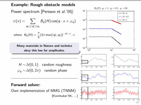
Example: Rough obstacle models
Power spectrum [Persson et al.’05]:
ψ(x) =∑
q0≤|q|≤qs
Bq(H) cos(q · x + ϕq)
where Bq(H) =π
5(2πmax(|q|, ql ))−H−1 →
Many materials in Nature and technics
obey this law for amplitudes.
H ∼ U(0, 1) random roughness
ϕq ∼ U(0, 2π) random phase
Forward solver:
Own implementation of MMG (TNNM)
[Kornhuber’94,. . . ]
100
101
102
10−5
10−4
10−3
10−2
10−1
Bq(H), q0 =1, qℓ =10 , qs =26
H=0
H=0.5
H=1
0 0.2 0.4 0.6 0.8 1
−2
0
2
0 0.05 0.1 0.15 0.2 0.25
−1.5
−1
−0.5
0 0.2 0.4 0.6 0.8 1
−2
0
2
4
0 0.05 0.1 0.15 0.2 0.25
−2
−1
0
1
0 0.2 0.4 0.6 0.8 1
−10
−5
0
5
0 0.05 0.1 0.15 0.2 0.25
−10
−5
0
5
28
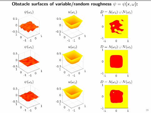
Obstacle surfaces of variable/random roughness ψ = ψ(x , ω):
29

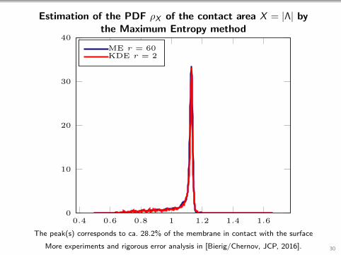
Estimation of the PDF ρX of the contact area X = |Λ| bythe Maximum Entropy method
0.4 0.6 0.8 1 1.2 1.4 1.60
10
20
30
40
ME r = 60
The peak(s) corresponds to ca. 28.2% of the membrane in contact with the surface
More experiments and rigorous error analysis in [Bierig/Chernov, JCP, 2016]. 30
Estimation of the PDF ρX of the contact area X = |Λ| bythe Maximum Entropy method
0.4 0.6 0.8 1 1.2 1.4 1.60
10
20
30
40
ME r = 60KDE r = 2
The peak(s) corresponds to ca. 28.2% of the membrane in contact with the surface
More experiments and rigorous error analysis in [Bierig/Chernov, JCP, 2016]. 30
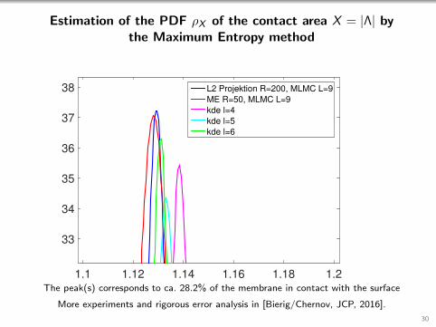
Estimation of the PDF ρX of the contact area X = |Λ| bythe Maximum Entropy method
1.1 1.12 1.14 1.16 1.18 1.2
33
34
35
36
37
38 L2 Projektion R=200, MLMC L=9
ME R=50, MLMC L=9
kde l=4
kde l=5
kde l=6
The peak(s) corresponds to ca. 28.2% of the membrane in contact with the surface
More experiments and rigorous error analysis in [Bierig/Chernov, JCP, 2016].
30
Summary:
Rigorous convergence analysis for the MLMC-MaximumEntropy Method for compactly suported densities
Num. experiments: smoothness assumptions may be relaxed
Open issue: how to select the number of moment constraints Rin practical computations (in the pre-asymptotic regime)?Adaptivity?
With appropriate R the method is able to produce goodapproximations for a broad class of densities.
Thank you for your attention!
31
References:
C. Bierig and A. Chernov, Approximation of probabilitydensity functions by the Multilevel Monte Carlo MaximumEntropy method, J. Comput. Physics, 314 (2016), 661–681
M. B. Giles, T. Nagapetyan, and K. Ritter, MultilevelMonte Carlo Approximation of Distribution Functions and Den-sities, SIAM/ASA J. Uncert. Quantif., 3 (2015), pp. 267–295
32
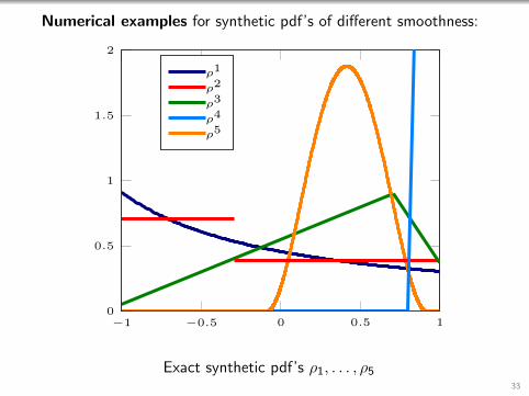
Numerical examples for synthetic pdf’s of different smoothness:
−1 −0.5 0 0.5 10
0.5
1
1.5
2
ρ1
ρ2
ρ3
ρ4
ρ5
Exact synthetic pdf’s ρ1, . . . , ρ533
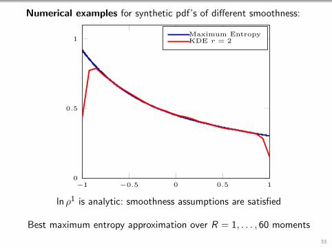
Numerical examples for synthetic pdf’s of different smoothness:
−1 −0.5 0 0.5 10
0.5
1Maximum EntropyKDE r = 2
ln ρ1 is analytic: smoothness assumptions are satisfied
Best maximum entropy approximation over R = 1, . . . , 60 moments
33
Numerical examples for synthetic pdf’s of different smoothness:
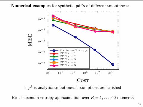
103 104 105 106 107 108
10−5
10−4
10−3
10−2
10−1
Cost
MISE
Maximum EntropyKDE r = 1KDE r = 2KDE r = 3KDE r = 4KDE r = 5
ln ρ1 is analytic: smoothness assumptions are satisfied
Best maximum entropy approximation over R = 1, . . . , 60 moments
33
Numerical examples for synthetic pdf’s of different smoothness:
−1 −0.5 0 0.5 10
0.5
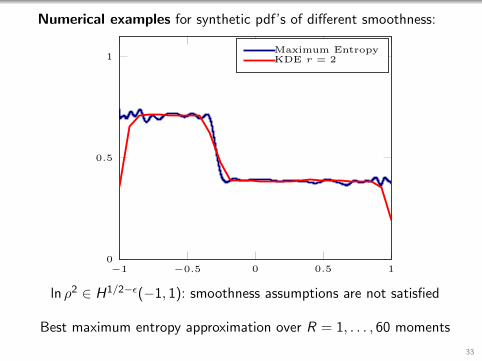
1Maximum EntropyKDE r = 2
ln ρ2 ∈ H1/2−ε(−1, 1): smoothness assumptions are not satisfied
Best maximum entropy approximation over R = 1, . . . , 60 moments
33
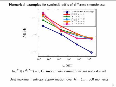
Numerical examples for synthetic pdf’s of different smoothness:
103 104 105 106 107 108
10−3
10−2
10−1
Cost
MISE
Maximum EntropyKDE r = 1KDE r = 2KDE r = 3KDE r = 4KDE r = 5
ln ρ2 ∈ H1/2−ε(−1, 1): smoothness assumptions are not satisfied
Best maximum entropy approximation over R = 1, . . . , 60 moments
33
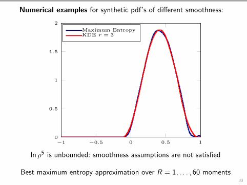
Numerical examples for synthetic pdf’s of different smoothness:
−1 −0.5 0 0.5 10
0.5
1
1.5
2
Maximum EntropyKDE r = 3
ln ρ5 is unbounded: smoothness assumptions are not satisfied
Best maximum entropy approximation over R = 1, . . . , 60 moments33
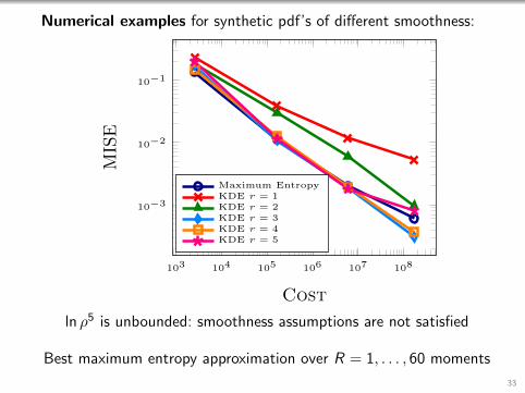
Numerical examples for synthetic pdf’s of different smoothness:
103 104 105 106 107 108
10−3
10−2
10−1
Cost
MISE
Maximum EntropyKDE r = 1KDE r = 2KDE r = 3KDE r = 4KDE r = 5
ln ρ5 is unbounded: smoothness assumptions are not satisfied
Best maximum entropy approximation over R = 1, . . . , 60 moments
33
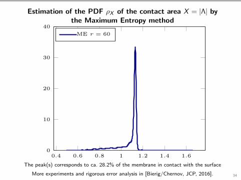
Estimation of the PDF ρX of the contact area X = |Λ| bythe Maximum Entropy method
0.4 0.6 0.8 1 1.2 1.4 1.60
10
20
30
40
ME r = 60
The peak(s) corresponds to ca. 28.2% of the membrane in contact with the surface
More experiments and rigorous error analysis in [Bierig/Chernov, JCP, 2016]. 34

Estimation of the PDF ρX of the contact area X = |Λ| bythe Maximum Entropy method
0.4 0.6 0.8 1 1.2 1.4 1.60
10
20
30
40
ME r = 60KDE r = 2
The peak(s) corresponds to ca. 28.2% of the membrane in contact with the surface
More experiments and rigorous error analysis in [Bierig/Chernov, JCP, 2016]. 34